Article

Real-Time Prediction of S-Wave Accelerograms from P-Wave Signals Using LSTM Networks with Integrated Fragility-Based Structural Damage Alerts for Induced Seismicity

by
Konstantinos G. Megalooikonomou
1,* and
Grigorios N. Beligiannis
1,2
1
School of Science and Technology, Hellenic Open University, Parodos Aristotelous 18, 26335 Patras, Greece
2
Department of Food Science & Technology, University of Patras, Agrinio Campus, G. Seferi 2, 30100 Agrinio, Greece
*
Author to whom correspondence should be addressed.
Appl. Sci. 2025, 15(20), 11017; https://doi.org/10.3390/app152011017 (registering DOI)
Submission received: 1 September 2025 / Revised: 7 October 2025 / Accepted: 11 October 2025 / Published: 14 October 2025
(This article belongs to the Special Issue Machine Learning Applications in Earthquake Engineering)

Abstract

Early warning of structural damage from induced seismic events requires rapid and reliable ground motion forecasting. This study presents a novel real-time framework that couples a deep learning approach with structural fragility assessment to generate immediate damage alerts following the onset of seismic shaking. Long Short-Term Memory (LSTM) neural networks are employed to predict full S-wave accelerograms from initial P-wave inputs, trained and tested on accelerometric records from induced seismicity scenarios. The predicted S-wave motion is then used as input for a suite of fragility curves in real time to estimate the probability of structural damage for masonry buildings typical in rural areas of geothermal platforms. The proposed method captures both the temporal evolution of shaking and the structural response potential, offering critical seconds of lead time for automated decision-making systems. Results demonstrate high predictive accuracy of the LSTM model and effective early classification of structural risk. This integrated system provides a practical tool for early warning or rapid response in regions experiencing anthropogenic seismicity, such as those affected by geothermal operations.

1. Introduction

Human-induced earthquakes represent a critical challenge, with implications for industries including geothermal energy, oil and gas, water management, mining, and waste disposal. Ongoing research focuses on global monitoring efforts, documenting case studies, advancing monitoring technologies, uncovering the underlying physical processes, improving forecasting with machine learning (ML) techniques, mitigating associated risks, estimating the maximum potential earthquake magnitude, and evaluating both impacts and stakeholder perspectives [1,2].
When an earthquake rupture is triggered, an earthquake early warning (EEW) or rapid response system can issue alerts that provide from a few seconds up to tens of seconds of lead time before damaging seismic waves arrive. Regional EEW methods estimate the earthquake’s magnitude and location using data from multiple seismic stations, whereas on-site EEW methods assess intensity or identify damaging earthquakes using data from a single station. Both regional (e.g., [3,4,5,6]) and on-site (e.g., [7,8,9]) approaches have successfully issued alerts during major earthquakes. In some cases, on-site methods have achieved longer lead times for regions located close to the epicenter (e.g., [8,9]). More recently, many EEW systems have adopted hybrid approaches that combine features of both techniques (e.g., [10,11,12]). The development and performance of these EEW strategies and systems have been summarized in several recent review papers (e.g., [13,14,15]).
In order to predict seismic intensity [peak ground acceleration (PGA) and peak ground velocity (PGV)], during the earliest stage of seismic-wave detection, artificial intelligence (AI) techniques have increasingly been applied, particularly in on-site EEW. Typically, several P-wave features are extracted from the initial waveforms after triggering and then used as input for prediction models built with AI methods. For example, the integration of the absolute values of acceleration, velocity, and displacement time histories—which provide a simplified description of waveform envelopes—has been applied in multilayer feedforward neural networks [16]. Similarly, features such as effective predominant period, cumulative absolute velocity, squared velocity integral, peak acceleration, peak velocity, and peak displacement have been used as inputs in models based on support vector regression (SVR) [17]. However, these approaches typically use only a subset of P-wave features, which may lead to the loss of important underlying waveform information. Moreover, new prediction models must be trained for different P-wave time-window lengths, with a common choice being around 3 s. These methods also neglect temporal variations within the P-waves, relying instead on aggregated values, thereby ignoring sequential characteristics in the data. Hsu and Huang et al. (2021) [18] used a deep convolutional neural network (CNN) to automatically extract informative features from P-wave recordings at a single station, enabling successful PGA prediction without significant information loss. Similarly, Chiang et al. (2022) [19] applied CNNs to extract initial P-wave features from a single station to determine whether the maximum PGA would exceed a predefined threshold. Fayaz and Galasso (2022) [20] developed a single-station approach using a deep neural network combined with a variational autoencoder to estimate acceleration response spectra, incorporating site characteristics and seven intensity measures. Jozinovic et al. (2020) [21] utilized a 10 s window of raw waveform data from multiple stations, starting at the earthquake origin time, along with a CNN, to predict PGA at distant stations that had not yet recorded peak shaking. More recently, Munchmeyer et al. (2021) [22] proposed a deep learning framework combining CNNs and transformer networks to process raw waveform data from an arbitrary number of stations at arbitrary locations, enabling predictions of both earthquake magnitude and location [23].
Long Short-Term Memory (LSTM) networks, a type of recurrent neural network (RNN), establish connections between past and present inputs. By selectively retaining information from previous time steps, the network incorporates it as additional input at the current step. This ability to capture temporal dependencies makes LSTM models highly effective for sequential data tasks, such as speech recognition [24], stock price prediction [25], and short-term traffic forecasting [26]. Building on this capability, Wang et al. (2020) [27] developed an LSTM-based neural network for on-site EEW.
To enable rapid forecasting of expected damage (or performance), appropriate fragility curves derived through probabilistic methods are essential. Using these performance levels, a tailored rapid damage forecasting system can be developed [28]. Such a system issues alerts based on predefined ground-motion thresholds, while accounting for the anticipated performance of one or more specific structures. Based on Figure 1, Long Short-Term Memory (LSTM) neural networks are utilized to forecast complete S-wave accelerograms based on initial P-wave recordings, with training and validation conducted using accelerometric data from induced seismicity events. The resulting S-wave predictions are subsequently fed into a set of fragility curves in real time based on Peak Ground Acceleration (PGA) values to assess the likelihood of structural damage for masonry buildings commonly found in rural geothermal areas. This approach effectively captures both the temporal development of ground shaking and the potential structural response, providing possible crucial lead time for automated decision-making systems.
This paper has the following contributions to the research area of ML methods in earthquake engineering:
  • Integrated real-time framework: Combines LSTM-based seismic wave prediction with structural fragility analysis to provide immediate, actionable damage alerts.
  • Advanced temporal modeling: Uses initial P-wave data to accurately forecast full S-wave accelerograms, capturing nonlinear ground motion evolution.
  • Rapid, validated risk estimation: Demonstrates high predictive accuracy and effective early classification of structural damage, offering possible crucial lead time for automated decision-making in induced seismicity scenarios.
The structure of this study is the following: after the introduction, which describes the initiatives of this research paper, the employed data and the performed methodology are described in Section 2. The steps of the performed supervised ML method in Python programming language (Version 3.12) and its output results are provided in Section 2 and Section 3. Finally, the discussion of the latter results is presented in Section 4, while the conclusions and future work are presented in Section 5.

2. Materials and Methods

2.1. Induced Ground Motion Database

The Pacific Earthquake Engineering Research Center (PEER) [29] hosts a web-based ground motion database that enables users to search, select, and download ground motion records. For evaluating the real-time prediction of S-wave accelerograms from P-wave signals using LSTM networks—combined with fragility-based structural damage alerts for induced seismicity—realistic induced ground motion records are required [28].
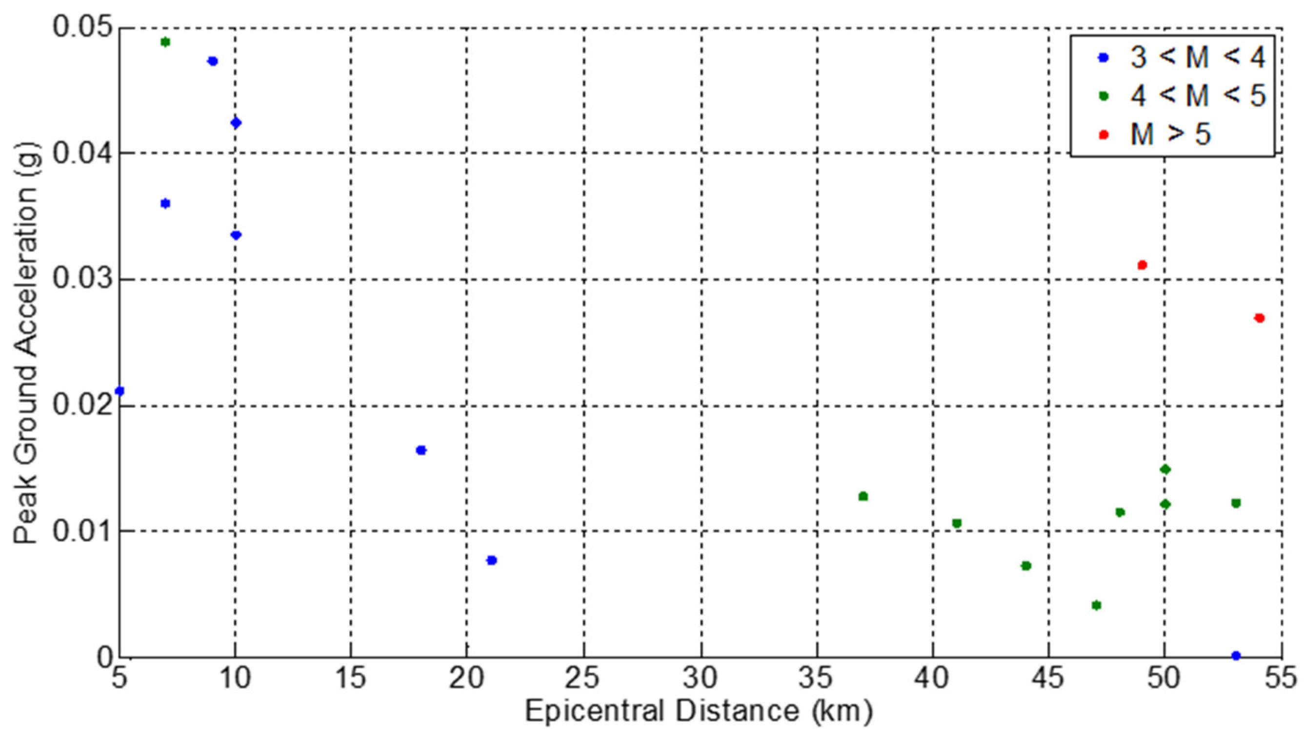
To address this, the PEER database was examined for induced ground motion events, and 20 records were selected. In total, nine induced earthquakes were identified, primarily occurring in Oklahoma, Arkansas, and Texas, USA (Table 1). These earthquakes were shallow, with depths between 3 and 14 km. From the available stations, records closest to the epicenter were chosen, with epicentral distances ranging from 5 km (the nearest station) to 55 km. The selected events had moment magnitudes between 3.0 and 5.5 (Figure 2), and the corresponding range of PGA values is also shown in Figure 2.

2.2. Short-Term Average over Long-Term Average (STA/LTA) for Induced Seismic Event Detection

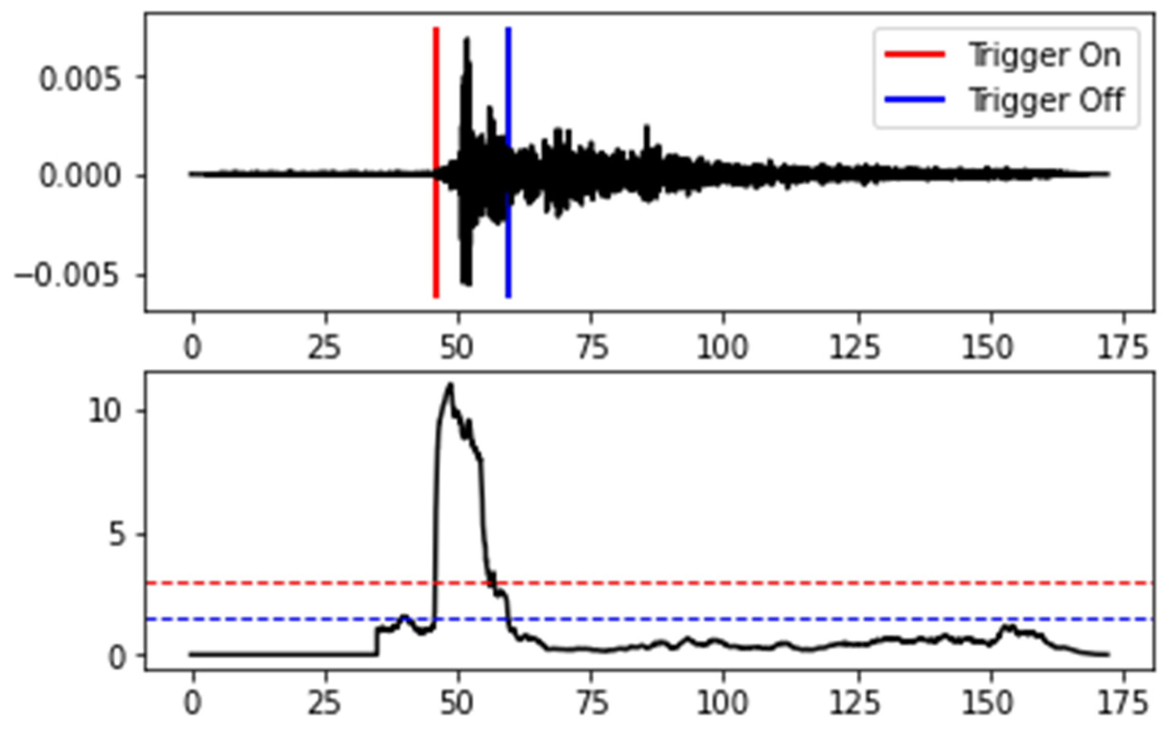
The short-term average over long-term average (STA/LTA) [30] is a signal processing technique commonly used in seismology and other time-series analysis fields for event detection (e.g., detecting earthquakes, acoustic events, or anomalies in continuous data streams). The STA/LTA ratio is a dimensionless measure that highlights sudden changes in a signal compared to its background. This method is applied to the induced ground motions of the database (Table 1) in order to define the P-wave arrival time and when the event’s trigger is on and off (P-waves are first; the trigger-on usually matches the P-wave arrival, and the trigger-off occurs after the higher-energy S-wave has passed). Figure 3 depicts these parameters for the ground motion of the North–South horizontal component of the station GS OK009 in the Arcadia event of Table 1 in 2010, along with its characteristic function.

2.3. Description and Input–Output Design of LSTM Machine Learning Model

LSTM (Long Short-Term Memory) RNNs are a specialized type of RNN Recurrent Neural Network designed to better capture long-term dependencies and sequential patterns in data. They also address common training challenges, such as the exploding gradient problem. Unlike a standard RNN layer, an LSTM layer replaces the simple RNN structure with units capable of identifying important correlations in the data, while “ignoring” irrelevant or noisy information. To illustrate the need for LSTM RNNs, consider a dataset where each record is a very long sentence. For this example, assume that each sentence-record is represented by a set of D variables, where each variable corresponds to a word in the sentence. The goal is to predict the last word of each sentence, and D represents the total number of words in the longest sentence-record. In a dataset with D variables, a single-layer LSTM RNN operates similarly to a standard RNN, as shown in Figure 1. The key difference is the presence of an additional set of outputs (C1, C2,…,CD), which are fed into the layer when processing the next variable. In the sentence example, these outputs indicate whether the immediately preceding word is “important” or should be ignored when predicting the next word. Training an LSTM RNN follows the same procedure as training a standard RNN, with the added step of estimating these values (C1, C2,…,CD). The network uses the known target values in the training data to learn optimal network parameters and determine the significance values C1, C2,…,CD for each position in a sequence. Once trained, an LSTM RNN can predict new data, and is particularly well-suited for tasks that require learning long-range dependencies, much like a standard RNN, but with greater efficiency and reliability [31].
Similarly, and according to Figure 1, the recorded ground motion of a horizontal component from the seismic station near the induced seismic event from the PEER database is divided in the P-wave signal, until the first important acceleration peaks of S-wave arrival and the rest until trigger-off (based on the previous subsection’s remarks) are considered as an S-wave accelerogram. The P-wave signal is used as an input for training the LSTM neural network and the S-wave accelerogram is used for testing the predictions of the LSTM RNN network. One part of the S-wave accelerogram is used also for the validation set of this machine learning method.
Finally, machine learning models and neural networks are trained to accept a set of values X (the values of the available variables) in order to predict the value of the variable Y. However, in the present problem of forecasting future values of a variable, there is only one variable available—acceleration values—which is the one whose future values must be predicted as Y. This problem can be overcome by applying a simple transformation to the data. Specifically, from the original time-series data, new data is created. In this data, each record contains one of the available values of the variable as the true label variable to be predicted and past values of the same variable as the remaining available variables (see Figure 4 of a random variable of this data process). The time-series data, consisting of sequential observations of the variable Y, is transformed into a supervised learning format using a sliding-window approach. Specifically, lagged values of Y are constructed as predictor variables (Xi) where each Xi corresponds to the value of Y at previous time steps. The target variable is defined as the current value of Y. This restructuring enables the use of regression or machine learning algorithms by mapping past observations to predict future outcomes, thereby converting the forecasting task into a supervised learning problem. In the next section, the results of this machine learning method applied to the PEER database through LSTM networks will be provided for the considered ground motions (Table 1).

3. Results

3.1. Application of LSTM RNN Network with Python

Following the description of the proposed methodology, this section presents the results of applying machine learning (ML) techniques to rapid response systems for induced seismicity near geothermal platforms. The analysis focuses on supervised ML methods, with particular emphasis on LSTM RNNs, applied to a subset of the PEER database (Table 1).
The standard workflow of a machine learning task generally involves the following steps:
  • Formulating the problem and identifying the required data.
  • Collecting the data in a usable format.
  • Detecting and addressing data gaps or uncertainties.
  • Preprocessing and preparing the data for model input.
  • Training the model on the designated training dataset.
  • Using the trained model to generate predictions on the test dataset.
  • Comparing the predictions with the actual test outcomes and calculating performance metrics.
  • Refining the model, expanding the dataset, or considering alternative modeling strategies if results are not satisfactory.
Neural networks are computational models inspired by the functioning of the human brain, designed to address a wide range of tasks such as classification, regression, and time-series forecasting. The branch of machine learning dedicated to training neural networks—particularly those with complex architectures—is commonly referred to as Deep Learning [31]. The fundamental unit of a neural network is the neuron. In essence, a neural network is composed of interconnected neurons organized into multiple layers.
Training an LSTM RNN on the available dataset involves optimizing the parameters that link neurons between successive layers. In this study, the LSTM layer consists of 500 neurons. The training process, which begins with forward propagation, can be outlined as follows:
  • Each record in the training set is passed through the LSTM RNN, and the network produces a prediction of the target variable.
  • These predictions are then used to compute the Cost Function, which measures the prediction error of the model. A commonly used choice is the Mean Squared Error (MSE).
  • Following forward propagation, backward propagation is performed. In this step, the model’s parameters are updated to reduce the Cost Function value. The updates are carried out in reverse order—starting from the output layer and moving back toward the input layer.
  • The combination of forward propagation, cost calculation, and backward propagation for the entire training set constitutes a single epoch.
  • The next epoch begins using the updated parameters from the previous iteration. Training continues for the specified number of epochs, and the parameter values obtained after the final backward propagation are taken as the trained LSTM RNN model parameters.
It should be emphasized that the number of epochs (set to 1000 in this study) is chosen by the analyst, and represents a hyperparameter of the LSTM RNN model. Typically, the appropriate number of epochs is determined through trial and error. In general, using too few epochs may result in underfitting, as the model has insufficient exposure to the training data, while too many epochs can lead to overfitting, where the model becomes overly tailored to the training set and performs poorly on unseen data.
Mathematically, training a neural network—similar to any supervised learning model—can be formulated as the problem of minimizing a chosen cost function with respect to the model parameters. In the case of an LSTM RNN, these parameters represent the weights that connect the outputs of neurons in one layer to the inputs of neurons in the subsequent layer. Since this optimization problem is typically too complex to be solved exactly using closed-form solutions, numerical methods are employed in practice. The process is further facilitated by optimization algorithms, which systematically guide the search for parameter values that minimize the cost function.
The Adaptive Moment Estimation (Adam) algorithm, employed in this study, is among the most widely used optimization methods in neural network training. Unlike algorithms that apply a single learning rate to all parameters, Adam assigns an individual learning rate to each parameter. This feature makes it particularly effective for handling complex and noisy datasets, enabling faster convergence and making it a preferred choice for training neural networks on challenging problems.
Selecting an appropriate activation function for the neurons in the LSTM layers is a critical step in the development of a neural network model. The choice of activation function depends on the specific task the network is designed to address (e.g., regression or classification), as well as on whether it is applied within the hidden/LSTM layers or at the output layer. Table 2, below, provides a summary of the activation function used in this study.
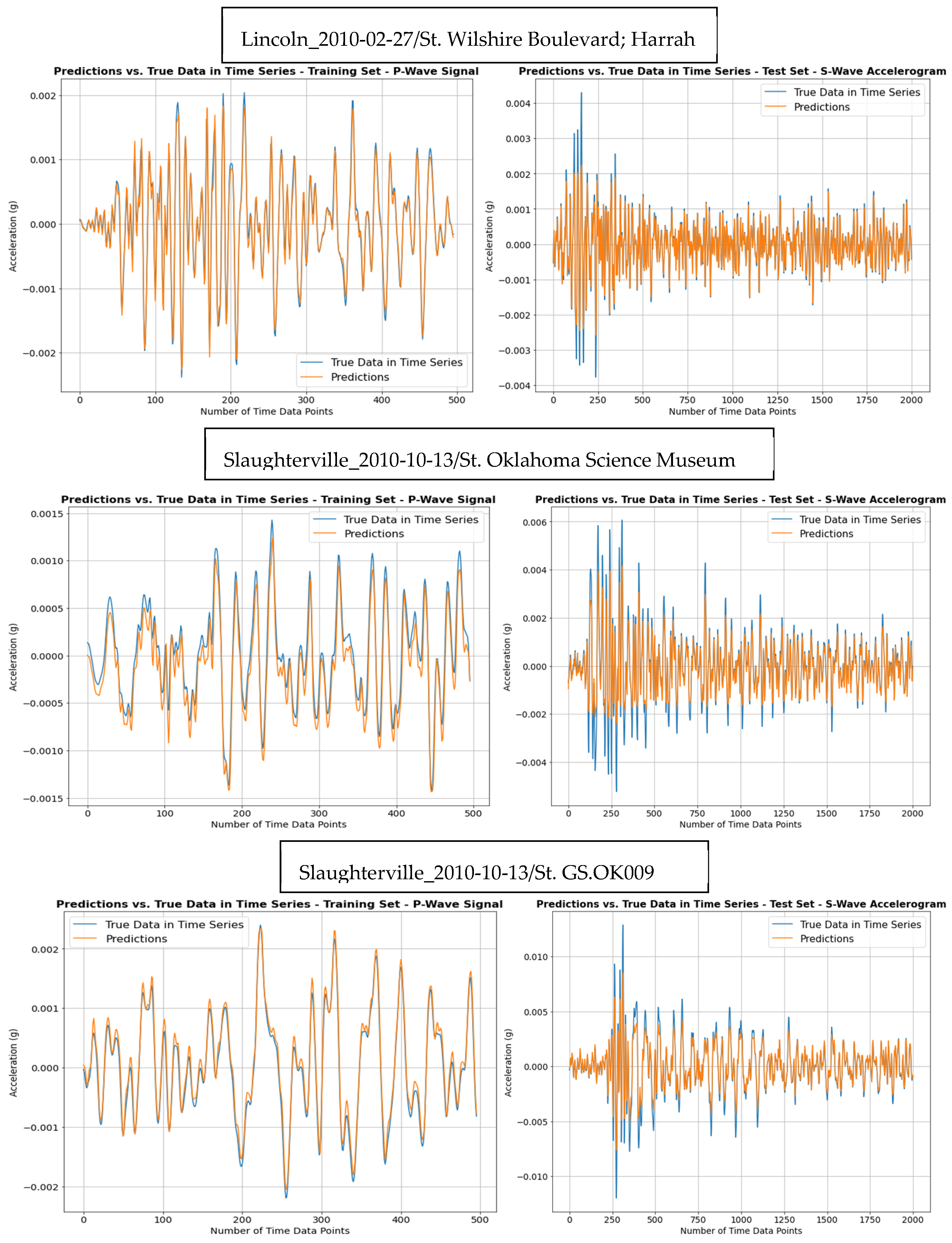
An essential hyperparameter in training a neural network is the choice of the cost function. As previously discussed, the training process aims to determine the optimal parameter values that minimize this function. So far, particular reference has been made to the Mean Squared Error (MSE). Table 3 presents the cost function employed in this study for the regression problem under consideration. So, to sum up, in the proposed model there is an LSTM layer with 500 neurons and ReLu activation function. Moreover, there is a hidden layer of 500 neurons with the same activation function. Finally, there is an output layer of 1 neuron without an activation function. The performance of the proposed methodology applied to some of the induced ground motions (to avoid repetition) of Table 1 of the PEER database is depicted in the following Figure 5 for ML training and testing, along with some metrics reported in Table 4.
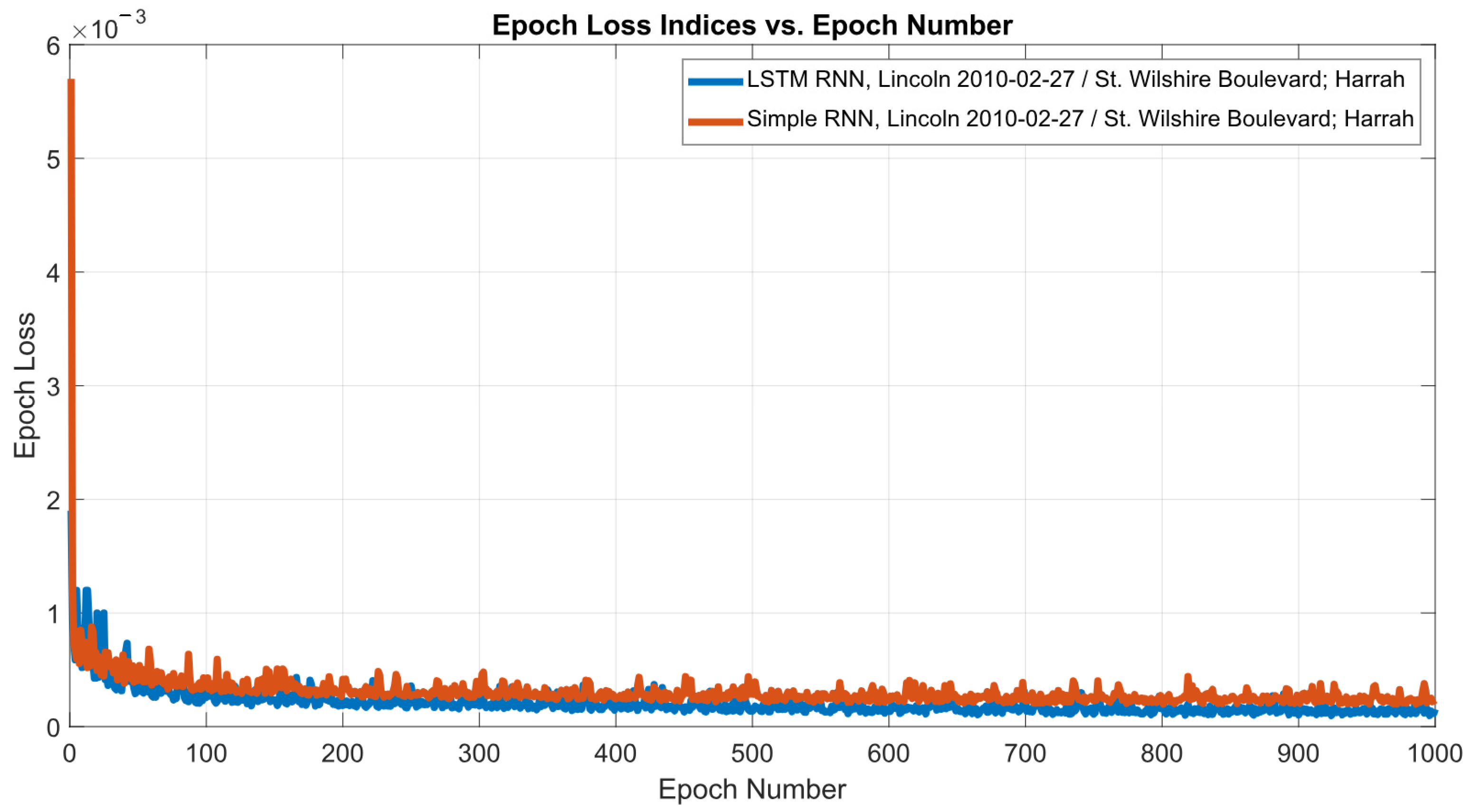
Finally, in Figure 6, the loss indices depending on the number of epochs are reported for Lincoln_2010-02-27/St. Wilshire Boulevard; Harrah ground motion, to justify the epoch number selection from the learning rate. The graph illustrates the training loss of an LSTM network over 1000 epochs, showing its performance in forecasting based on time-series data from “Lincoln 2010-02-27/St. Wilshire Boulevard; Harrah.” The loss, which measures the model’s prediction error, starts on relatively high, at around 2 × 10⁻³, and decreases rapidly in the initial epochs, indicating effective learning during early training. As training progresses, the loss continues to decline more gradually and stabilizes with minor fluctuations, suggesting the model is converging and fine-tuning its predictions. Overall, the steadily decreasing loss demonstrates that the LSTM network is successfully learning temporal patterns in the data and improving its forecasting accuracy over time. Finally, in the last figure, a comparison of a standard RNN with LSTM RNN is added, with the same neural network layers’ configuration. While both are recurrent architectures, the standard RNN suffers from vanishing gradient limitations, which reduce its ability to capture longer temporal dependencies. As expected, in this experiment the standard RNN underperformed, showing noticeably higher loss (Figure 6) and less accuracy. In contrast, the LSTM RNN achieved significantly lower error values (simple RNN had an MSE of 0.0001133 in training and 0.0001001 in testing, accordingly) and can provide through PGA more reliable fragility-based damage alerts. This direct comparison within the RNN family demonstrates that while a simple RNN can be applied to the problem, the LSTM’s gating mechanisms yield substantially better performance, making it the more suitable choice.

3.2. Adopted Fragility Curves near Geothermal Platforms in France

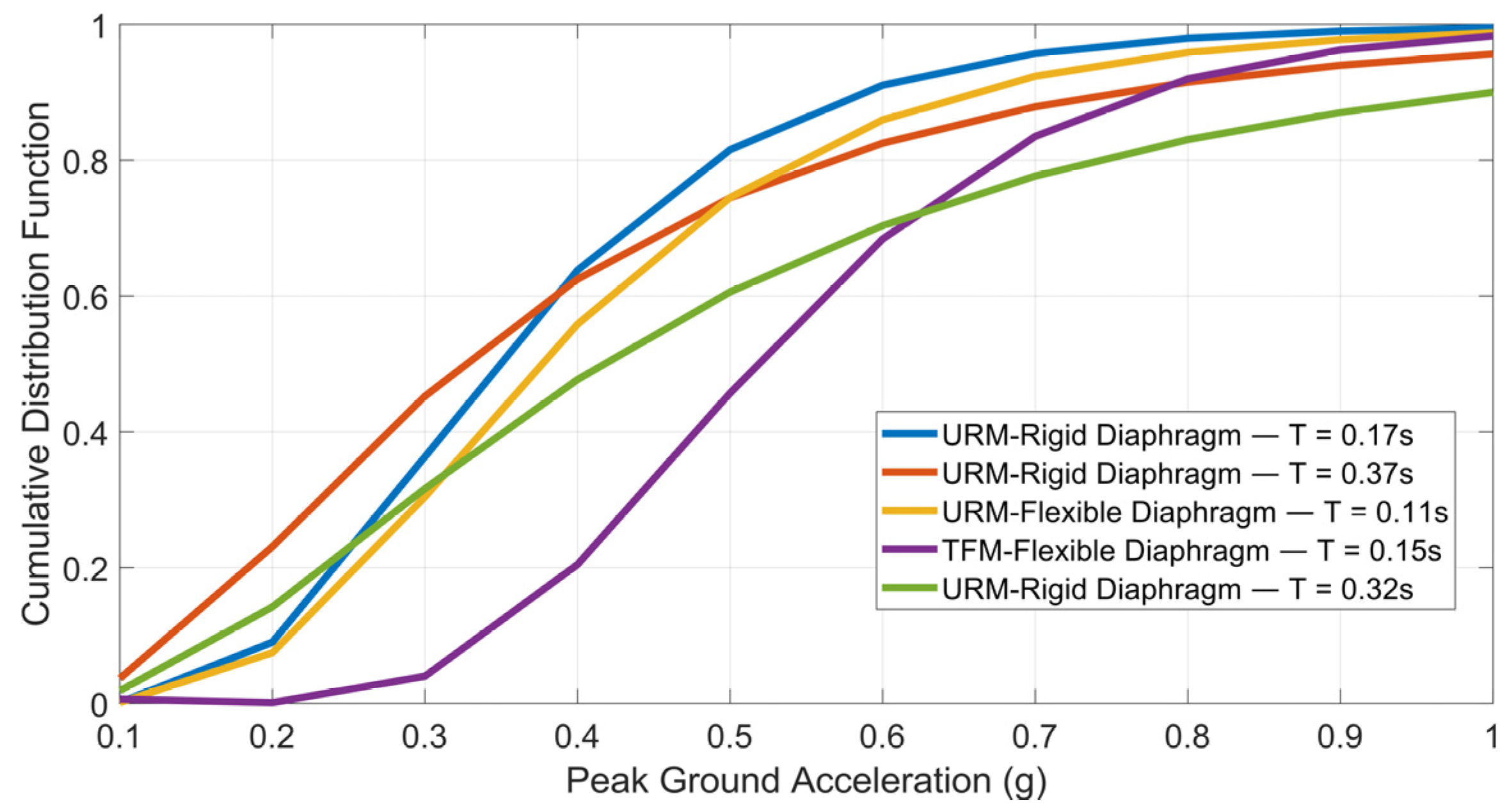
Based on real case studies of Timber-Framed Masonry (TFM) and Unreinforced Masonry (URM) buildings in Alsace, France [28], fragility curves were developed in terms of PGA through structural analysis, using incremental dynamic analysis (IDA) with gradually increasing seismic intensity [32]. The analysis of the equivalent single-degree-of-freedom (ESDOF) models [33] for these buildings was carried out in MATLAB (R2024b) [34], with the FEDEAS Lab toolbox [35]. Ground motion records obtained from the previously introduced PEER database (Table 1) were applied in the transverse (short/weak) direction of the building plans. The fundamental periods of the studied structures were validated through ambient vibration measurements using floor-level sensors [36] installed in each building [28]. In addition, the main geometric data required for the simplified vulnerability models were collected during on-site inspections [28,37]. The resulting fragility curves for slight damage common in induced seismic events are presented in Figure 7. They show that URM buildings exhibit a relatively similar probability of damage across different intensities, whereas the more earthquake-resistant TFM buildings demonstrate reduced fragility at low-to-medium intensity levels.

4. Discussion

Modern early-warning strategies for induced seismicity increasingly integrate real-time monitoring, machine learning, and physics-based statistical models. The traditional “traffic-light system”—which adjusts industrial operations based on observed seismic thresholds—is still widely used, yet it has limitations, like delayed responses and post-shutdown events (DESTRESS H2020, 2020 [37]). Cutting-edge advancements are enhancing predictive capabilities through deep learning models trained on datasets from geothermal sites. Complementary approaches include statistical forecasting models to predict the maximum expected magnitude in near-real time, and guide mitigation strategies [2,22]. These combined strategies represent the current frontier: leveraging high-resolution monitoring data, AI-driven early detection, and probabilistic forecasting to improve the timeliness and precision of induced seismicity warnings. In this study however, fragility-based alert systems, which link ground-motion LSTM RNN networks predictions from real induced seismic events directly to the vulnerability (fragility curves) of nearby infrastructure, are allowing operators to issue warnings not based on seismic magnitude, but on the probability of exceeding seismic damage thresholds (Figure 1 and Figure 7). From the results of Figure 5 and Table 4, it can be seen that, although there is some deviation in the PGA (making the rapid response system more conservative through the fragility curves of Figure 1 and Figure 7), the overall capture of the nonlinearity of the ground motion has a minimum MSE error. This deviation in PGA values in the testing set is due to the fact that the ML model is not trained to high PGA values from the P-wave signal. Finally, it should be noted that CNNs and RNNs offer complementary strengths for EEW systems. CNNs excel at extracting spatial and temporal features from seismic waveforms, making them effective for rapid event detection and classification directly from raw sensor data. They can quickly identify patterns associated with P-waves, enabling faster alerts [18,22]. In contrast, RNNs, particularly those using LSTM architectures, are well-suited for modeling sequential dependencies and predicting the evolution of seismic signals over time. This makes RNNs valuable for estimating parameters such as earthquake magnitude or predicting ground motion progression. In practice, CNNs often outperform RNNs in speed and robustness, while RNNs provide better temporal context—leading to hybrid CNN-RNN models that leverage both spatial feature extraction and temporal sequence learning for improved EEW accuracy and reliability. Therefore, future work would apply the research framework of Figure 1 to hybrid CNN-RNN models.

5. Conclusions

A reliable performance-based monitoring framework offers an effective approach to managing risks from induced and triggered seismicity. To enable rapid loss forecasting, a set of fragility curves for slight damage in masonry buildings has been adopted from previous authors’ research. The improved real-time rapid response system leverages LSTM neural networks to predict complete S-wave accelerograms from the initial P-wave inputs of real induced seismic events drawn from the developed subset of the PEER database. The STA/LTA ratio—a dimensionless measure that highlights sudden changes in a signal compared to its background—is applied to the induced ground motions of the database in order to define the P-wave arrival time and when the event’s trigger is on and off (P-waves are first; the trigger-on usually matches the P-wave arrival, and the trigger-off occurs after the higher-energy S-wave has passed). Then, the predicted S-wave motions are connected through PGA prediction to the fragility curves in real time, to estimate the probability of structural damage in masonry buildings commonly found in rural geothermal regions. By capturing, with minimal error, the nonlinear evolution of ground shaking, and connecting that to the corresponding structural response, the method could provide critical seconds of lead time for automated decision-making systems. This capability enhances risk awareness for local stakeholders and industry alike, contributing to more informed and effective management of risks associated with induced and triggered seismicity. This study will be the basis for further examination of hybrid CNN-RNN models that synergistically combine spatial feature extraction and temporal sequence learning to boost EEW performance and reliability.

Author Contributions

Conceptualization, K.G.M.; data curation, K.G.M.; formal analysis, K.G.M. and G.N.B.; investigation, K.G.M.; methodology, K.G.M. and G.N.B.; project administration, G.N.B.; resources, K.G.M.; software, K.G.M.; supervision, G.N.B.; validation, K.G.M. and G.N.B.; visualization, K.G.M.; writing—original draft, K.G.M.; writing—review and editing, G.N.B. All authors have read and agreed to the published version of the manuscript.

Funding

This research received no external funding.

Informed Consent Statement

Not applicable.

Data Availability Statement

All data included in this study are available from a publicly accessible repository.

Acknowledgments

The present research work is partially based on previous research by the corresponding author and his participation in the European Union-funded project DESTRESS (H2020-Work Package 3.4) [28,37].

Conflicts of Interest

The authors declare no conflicts of interest.

Abbreviations

The following abbreviations are used in this manuscript:
EEWEarthquake Early Warning
PEERPacific Earthquake Engineering Research Center
LSTMLong Short-Term Memory neural network
CNNConvolutional Neural Network
RNNRecurrent Neural Network
PGAPeak Ground Acceleration
AIArtificial Intelligence
MLMachine Learning
STA/LTAShort-Term Average over Long-Term Average
TFMTimber-Framed Masonry
URMUnreinforced Masonry
ESDOFEquivalent Single-Degree-Of-Freedom
MSEMean Squared Error
MAEMean Absolute Error

References

  1. Zhou, W.; Lanza, F.; Grigoratos, I.; Schultz, R.; Cousse, J.; Trutnevyte, E.; Muntendam-Bos, A.; Wiemer, S. Managing induced seismicity risks from enhanced geothermal systems: A good practice guideline. Rev. Geophys. 2024, 62, e2024RG000849. [Google Scholar] [CrossRef]
  2. Qin, Y.; Chen, T.; Ma, X.; Chen, X. Forecasting induced seismicity in Oklahoma using machine learning methods. Sci. Rep. 2022, 12, 9319. [Google Scholar] [CrossRef] [PubMed]
  3. Fujinawa, Y.; Noda, Y. Japan’s Earthquake Early Warning System on 11 March 2011: Performance, Shortcomings, and Changes. Earthq. Spectra 2013, 29, S341–S368. [Google Scholar] [CrossRef]
  4. Cuéllar, A.; Espinosa-Aranda, J.M.; Suarez, R.; Ibarrola, G.; Uribe, A. The Mexican Seismic Alert System (SASMEX): Its Alert Signals, Broadcast Results and Performance During the M 7.4 Punta Maldonado Earthquake of March 20th, 2012. In Early Warning for Geological Disasters; Wenzel, F., Zschau, Z., Eds.; Springer: Berlin/Heidelberg, Germany, 2014; pp. 71–87. [Google Scholar]
  5. Yamada, M.; Tamaribuchi, K.; Wu, S. Faster and More Accurate Earthquake Early Warning System. J. Jpn. Assoc. Earthq. Eng. 2014, 14, 21–24. [Google Scholar] [CrossRef]
  6. Kodera, Y.; Saitou, J.; Hayashimoto, N.; Adachi, S.; Morimoto, M.; Nishimae, Y.; Hoshiba, M. Earthquake Early Warning for the 2016 Kumamoto Earthquake: Performance Evaluation of the Current System and the Next-Generation Methods of the Japan Meteorological Agency. Earth Planets Space 2016, 68, 202. [Google Scholar] [CrossRef]
  7. Hsu, T.-Y.; Wang, H.-H.; Lin, P.-Y.; Lin, C.-M.; Kuo, C.-H.; Wen, K.-L. Performance of the NCREE’s On-Site Warning System during the 5 February 2016Mw6.53 Meinong Earthquake. Geophys. Res. Lett. 2016, 43, 8954–8959. [Google Scholar] [CrossRef]
  8. Hsu, T.Y.; Lin, P.Y.; Wang, H.H.; Chiang, H.W.; Chang, Y.W.; Kuo, C.H. Comparing the Performance of the NEEWS Earthquake Early Warning System against the CWB System during the 6 February 2018 Mw 6.2 Hualien Earthquake. Geophys. Res. Lett. 2016, 45, 6001–6007. [Google Scholar]
  9. Wu, Y.M.; Mittal, H.; Huang, T.C.; Yang, B.M.; Jan, J.C.; Chen, S.K. Performance of a Low-Cost Earthquake Early Warning System (P-Alert) and Shake Map Production during the 2018 Mw 6.4 Hualien, Taiwan, Earthquake. Seismol. Res. Lett. 2019, 90, 19–29. [Google Scholar] [CrossRef]
  10. Kodera, Y.; Yamada, Y.; Hirano, K.; Tamaribuchi, K.; Adachi, S.; Hayashimoto, N.; Morimoto, M.; Nakamura, M.; Hoshiba, M. The Propagation of Local Undamped Motion (PLUM) Method: A Simple and Robust Seismic Wavefield Estimation Approach for Earthquake Early Warning. Bull. Seismol. Soc. Am. 2018, 108, 983–1003. [Google Scholar] [CrossRef]
  11. Kodera, Y. An Earthquake Early Warning Method Based on Huygens Principle: Robust Ground Motion Prediction Using Various Localized Distance-Attenuation Models. J. Geophys. Res. Solid Earth 2019, 124, 12981–12996. [Google Scholar] [CrossRef]
  12. Hsu, T.-Y.; Kuo, C.-H.; Wang, H.-H.; Chang, Y.-W.; Lin, P.-Y.; Wen, K.-L. The Realization of an Earthquake Early Warning System for Schools and its Performance during the 2019 ML 6.3 Hualien (Taiwan) Earthquake. Seismol. Res. Lett. 2021, 92, 342–351. [Google Scholar] [CrossRef]
  13. Allen, R.M.; Melgar, D. Earthquake Early Warning: Advances, Scientific Challenges, and Societal Needs. Annu. Rev. Earth Planet. Sci. 2019, 47, 361–388. [Google Scholar] [CrossRef]
  14. Cremen, G.; Galasso, C. Earthquake Early Warning: Recent Advances and Perspectives. Earth-Sci. Rev. 2020, 205, 103184. [Google Scholar] [CrossRef]
  15. Wald, D.J. Practical Limitations of Earthquake Early Warning. Earthq. Spectra 2020, 36, 1412–1447. [Google Scholar] [CrossRef]
  16. Böse, M.; Heaton, T.; Hauksson, E. Rapid Estimation of Earthquake Source and Ground-Motion Parameters for Earthquake Early Warning Using Data from a Single Three-Component Broadband or Strong-Motion Sensor. Bull. Seismol. Soc. Am. 2012, 102, 738–750. [Google Scholar] [CrossRef]
  17. Hsu, T.-Y.; Huang, S.-K.; Chang, Y.-W.; Kuo, C.-H.; Lin, C.-M.; Chang, T.-M.; Wen, K.-L.; Loh, C.-H. Rapid On-Site Peak Ground Acceleration Estimation Based on Support Vector Regression and P-Wave Features in Taiwan. Soil Dyn. Earthq. Eng. 2013, 49, 210–217. [Google Scholar] [CrossRef]
  18. Hsu, T.-Y.; Huang, C.-W. Onsite Early Prediction of PGA Using CNN with Multi-Scale and Multi-Domain P-Waves as Input. Front. Earth Sci. 2021, 9, 626908. [Google Scholar] [CrossRef]
  19. Chiang, Y.-J.; Chin, T.-L.; Chen, D.-Y. Neural Network-Based Strong Motion Prediction for On-Site Earthquake Early Warning. Sensors 2022, 22, 704. [Google Scholar] [CrossRef]
  20. Fayaz, J.; Galasso, C. A Deep Neural Network Framework for Real-Time On-Site Estimation of Acceleration Response Spectra of Seismic Ground Motions. Comput.-Aided Civ. Infrastruct. Eng. 2022, 38, 87–103. [Google Scholar] [CrossRef]
  21. Jozinović, D.; Lomax, A.; Štajduhar, I.; Michelini, A. Rapid Prediction of Earthquake Ground Shaking Intensity Using Raw Waveform Data and a Convolutional Neural Network. Geophys. J. Int. 2020, 222, 1379–1389. [Google Scholar] [CrossRef]
  22. Münchmeyer, J.; Bindi, D.; Leser, U.; Tilmann, F. The Transformer Earthquake Alerting Model: A New Versatile Approach to Earthquake Early Warning. Geophys. J. Int. 2021, 225, 646–656. [Google Scholar] [CrossRef]
  23. Hsu, T.Y.; Pratomo, A. Early Peak Ground Acceleration Prediction for On-Site Earthquake Early Warning Using LSTM Neural Network. Front. Earth Sci. 2022, 10, 911947. [Google Scholar] [CrossRef]
  24. Sak, H.; Senior, A.W.; Beaufays, F. Long Short-Term Memory Recurrent Neural Network Architectures for Large Vocabulary Speech Recognition. arXiv 2014, arXiv:1402.1128. [Google Scholar]
  25. Murtaza, R.; Patel, H.; Varma, S. Predicting Stock Prices Using LSTM. Int. J. Sci. Res. 2017, 6, 1754–1756. [Google Scholar]
  26. Zhao, Z.; Chen, W.; Wu, X.; Chen, P.C.Y.; Liu, J. LSTM Network: A Deep Learning Approach for Short-term Traffic Forecast. IET Intell. Transp. Syst. 2017, 11, 68–75. [Google Scholar] [CrossRef]
  27. Wang, C.Y.; Huang, T.C.; Wu, Y.M. A LSTM Neural Network for On-Site Earthquake Early Warning. EGU Gen. Assem. 2020, 2020, 3696. [Google Scholar]
  28. Megalooikonomou, K.G.; Parolai, S.; Pittore, M. Toward performance-driven seismic risk monitoring for geothermal platforms: Development of ad hoc fragility curves. Geotherm Energy 2018, 6, 8. [Google Scholar] [CrossRef]
  29. PEER-NGA-East Database; Pacific Earthquake Engineering Research Center. University of California: Berkeley, CA, USA, 2025. Available online: https://peer.berkeley.edu/research/nga-east (accessed on 5 June 2025).
  30. Beyreuther, M.; Barsch, R.; Krischer, L.; Megies, T.; Behr, Y.; Wassermann, J. ObsPy: A Python Toolbox for Seismology. Seismol. Res. Lett. 2010, 81, 530–533. [Google Scholar] [CrossRef]
  31. Burkov, A. The Hundred-Page Machine Learning Book. 2019. Available online: https://themlbook.com/ (accessed on 1 July 2025).
  32. Vamvatsikos, D.; Cornell, C.A. Incremental Dynamic Analysis. Earthq. Eng. Struct. Dyn. 2002, 31, 491–514. [Google Scholar] [CrossRef]
  33. Vamvatsikos, D.; Pantazopoulou, S.J. Development of a simplified mechanical model to estimate the seismic vulnerability of heritage unreinforced masonry buildings. J. Earthq. Eng. Taylor Fran 2015, 20, 298–325. [Google Scholar] [CrossRef]
  34. MATLAB: User’s Guide, Version R2024b; Mathworks Inc.: Natick, MA, USA, 2024.
  35. Filippou, F.C.; Constantinides, M. FEDEAS Lab—Getting Started Guide and Simulation Examples, NEESgrid Report 2004-22 and SEMM Report 2004-05, 2004. Available online: http://www.neesgrid.org/news/documents.php (accessed on 20 July 2025).
  36. Boxberger, T.; Fleming, K.; Pittore, M.; Parolai, S.; Pilz, M.; Mikulla, S. The Multi-Parameter Wireless Sensing System (MPwise): Its description and application to earthquake risk mitigation. Sensors 2017, 17, 2400. [Google Scholar] [CrossRef]
  37. DESTRESS: Demonstration of Soft Stimulation Treatments of Geothermal Reservoirs, EU Research Project H2020, 2020. Available online: https://www.destress-h2020.eu/en/home/ (accessed on 25 August 2025).
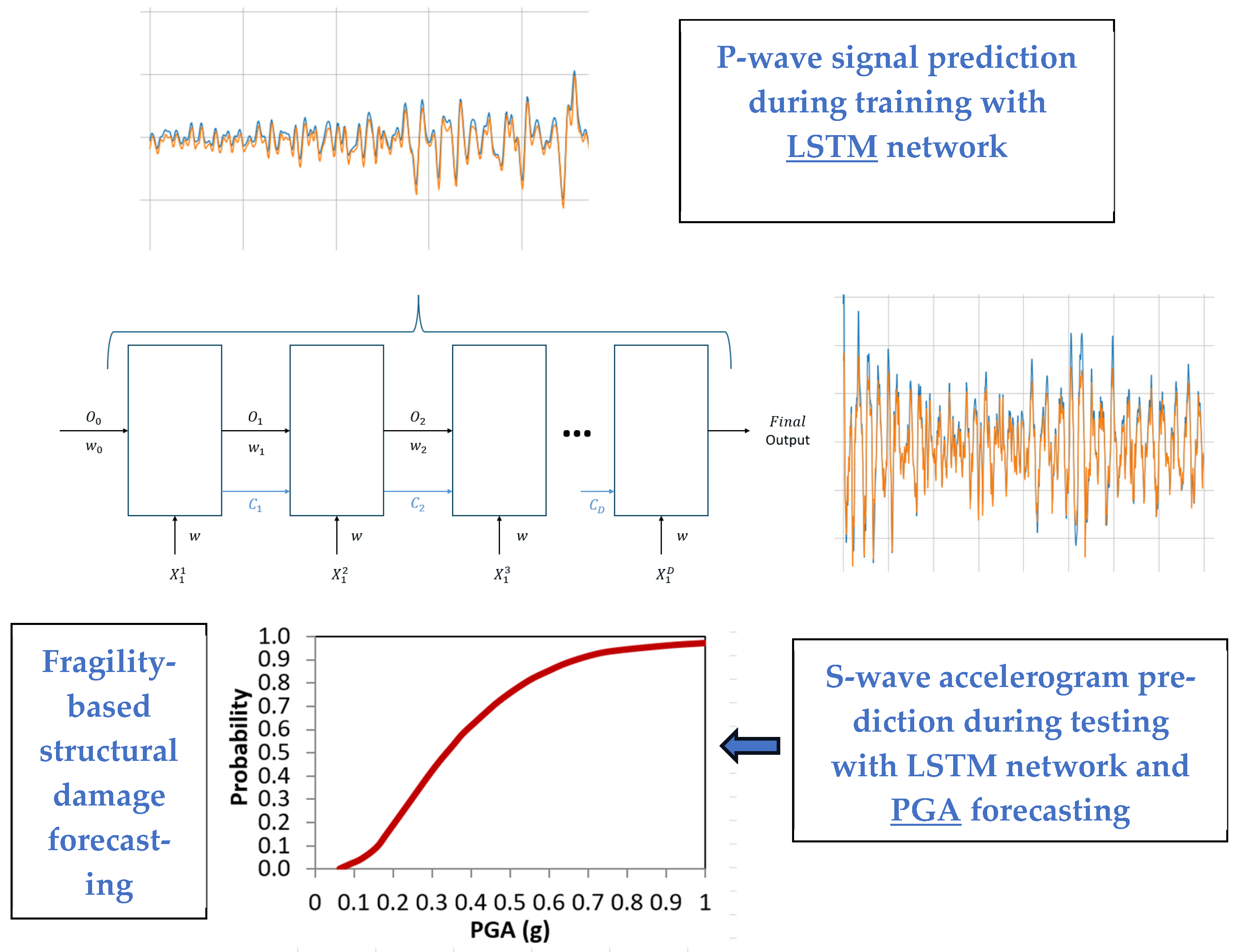
Figure 1. Graphical research framework of this study.
Applsci 15 11017 g001
Figure 2. Induced ground motions selected from PEER database.
Applsci 15 11017 g002
Figure 3. Trigger on and trigger off, along with the characteristic function of Arcadia-induced seismic event of Table 1 and the recorded accelerogram of station GS OK009 of PEER database (acceleration values in (g)).
Applsci 15 11017 g003
Figure 4. Data transformation for similar time-series (like ground motion) problems.
Applsci 15 11017 g004
Figure 5. Prediction of S-wave accelerograms (Horizontal 1/North–South component) from P-wave signals using LSTM RNN networks.
Applsci 15 11017 g005
Figure 6. Loss indices for Lincoln_2010-02-27/St. Wilshire Boulevard; Harrah ground motion for simple RNN and LSTM RNN.
Applsci 15 11017 g006
Figure 7. Fragility curves derived for TFM and URM real buildings near the geothermal platforms in Alsace, France.
Applsci 15 11017 g007
Table 1. Earthquake events involving induced seismicity identified in the PEER database.
EQ-IDEQ-ID DatabaseYearName LocationMwEpicenter Latitude (Deg)Epicenter Longitude (Deg)Depth (km)
1572010Lincoln_2010-02-27Lincoln OK4.1835.553−96.7524
2662010Slaughterville
_2010-10-13
Slaughterville OK4.3635.202−97.30914
3672010Guy_2010-10-15Guy AR3.8635.276−92.3225
4732010Arcadia_2010-11-24Arcadia OK3.9635.627−97.2463
5742010BethelAcres_
2010-12-12
Bethel Acres OK3.2335.392−96.9954
6762010Guy_2010-11-20Guy AR3.9035.316−92.3175
7802011Greenbrier_2011-02-28Greenbrier AR4.6835.265−92.344
8912011Sparks_2011-11-06Sparks OK5.6835.537−96.7479
9922011Comal_2011-10-20Comal TX4.7128.81−98.154
Table 2. Activations Function applied to the LSTM RNNs in this study.
Activation FunctionEquationApplication
ReLuF(x) = max(0, x)Regression problems with many hidden layers
Table 3. Cost Function of the LSTM RNN for the regression problem of this study.
Cost FunctionEquationApplication
Mean Absolute Error (MAE) M A E = 1 N i = 1 N Y i Y ^ i Regression problems: less strict compared to Mean Squared Error (MSE), since it does not quantify the error as the square of prediction’s deviation, but as an absolute distance.
Table 4. Mean Squared Error (MSE) of prediction performance of training and testing dataset.
EQ Name and Recording StationMSE Training SetMSE Testing Set
Lincoln_2010-02-27/St. Wilshire Boulevard; Harrah9.2268 × 10−57.1828 × 10⁻⁵
Slaughterville_2010-10-13/St. Oklahoma Science Museum0.00013740.0002488
Slaughterville_2010-10-13/St. GS.OK0090.00011150.0003106
Disclaimer/Publisher’s Note: The statements, opinions and data contained in all publications are solely those of the individual author(s) and contributor(s) and not of MDPI and/or the editor(s). MDPI and/or the editor(s) disclaim responsibility for any injury to people or property resulting from any ideas, methods, instructions or products referred to in the content.