Abstract
This work investigates the possibility to improve the computational efficiency of a set-based method for the trajectory planning of a car-like vehicle through artificial intelligence. Planning is performed on a graph that represents the operating scenario in which the vehicle moves, and the kinodynamic feasibility of the trajectories is guaranteed through a series of set-based arguments, which involve the solution of semi-definite programming problems. Navigation in the graph is performed through a hybrid A* algorithm whose performance metrics are improved through a properly trained classificator, which can forecast whether a candidate trajectory segment is feasible or not. The proposed solution is validated through numerical simulations, with a focus on the effects of different classificators features and by using two different kinds of artificial intelligence: a support vector machine (SVM) and a long-short term memory (LSTM). Results show up to a 28% reduction in computational effort and the importance of lowering the false negative rate in classification for achieving good planning performance outcomes.
1. Introduction
Among the various application areas, autonomous driving stands out for its strategic importance and the high level of innovation it demands. Trajectory planning consists of finding a sequence of positions, each one associated with a timed instant, from a starting position to a destination one [1]. It constitutes a key methodology across a wide range of technological domains, including robotics, advanced logistics, vehicular traffic, and the management of complex systems in dynamic environments, leading to intelligent urban transport networks. Industrial applications, such as the control of robotic arm movements [2,3,4] or the planning of routes for autonomous vehicles in automated warehouses [5,6], highlight the importance of optimizing trajectories under physical, dynamic, and safety constraints. In the evaluation of trajectories, another aspect that could be interesting to consider is the level of risk of the route, linked to environmental conditions, such as population density and hydrogeological risk. For example, an integrated risk model was proposed in [7]. Another area of growing interest lies in the management and prediction of airflow trajectories in confined environments [8,9], such as ventilation systems or environmental control frameworks. Here, trajectory planning principles can be applied to regulate flows efficiently, ensuring energy optimization and environmental comfort while addressing constraints similar to those found in mobility systems. These diverse contexts, along with many emerging applications, underscore the pivotal role of trajectory planning as a cross-disciplinary tool for tackling complex challenges. All the more so, this takes on primary importance in the context of smart cities, where the use of IoT technologies is strongly oriented toward process automation with the dual objective of maximizing energy efficiency and quality of service [10]. In this context, the European Union, through its latest directives, has set a clear goal of reducing greenhouse gasses emissions: initially by 30% and later increased to 55% by 2030 compared to 2021 levels. Achieving such an ambitious target cannot be reasonably accomplished without the widespread adoption of electric vehicles, the conscious and intelligent use of energy storage systems for electric traction [11], and the implementation of assisted and/or autonomous driving technologies.
The main push arises from its expected benefits, which include reducing incidents (94% of which are related to driver errors [12]) and emissions [13]. After years of extensive research, the SAE J3016[14] standard was finally published in 2014. This standard outlines six levels of vehicle automation (ranging from 0 to 5) for classification purposes. The third level, as defined by the SAE J3016, does not require constant human supervision and has been commercially available since the late 2010s. This level of automation is capable of performing complex safety-related tasks like lane-keeping with minimal human involvement [15]. Autonomous driving is a complex and interdisciplinary effort that involves finding solutions to a variety of challenges, particularly in urban environments [16]. The decision-making process in autonomous driving systems (ADSs) typically involves a layered approach that includes a local motion planning layer, which depends on the feedback control of vehicle systems [17]. This work tackles local motion planning, whose input is a structured environment in which both static and moving obstacles are represented by rectangular embeddings [18,19,20], hence assuming that a low-level control law exists, along with environment sensing and goals from the deliberative layer. Local motion planning is a foundational technology for autonomous driving, supporting the already commercially available J3016 level 2 features like self-parking, as well as level 3 applications where the automated driving system (ADS) handles intricate tasks within a specified operational design domain (ODD) with a human fallback, such as overtaking obstacles or slower vehicles. Motion planning for an autonomous driving system (ADS) usually consists of two phases [21,22]. The first phase is path planning, where an appropriate geometric path is determined between a starting position and a destination. The second phase involves associating this path with a suitable timing law [1]. From a computational perspective, these two phases can present significant challenges [23].
Numerous solutions have been proposed in the literature [24], many of which have been adapted from robotic motion planning techniques [25] or share similarities with Unmanned Aerial Vehicle (UAV) motion planning to some extent [26,27]. However, unlike robotic motion, autonomous vehicles have greater demands when it comes to performance and safety. Motion planning solutions can be categorized based on how they ensure the feasibility of trajectories, particularly in terms of adhering to specific constraints. For instance, some solutions are grounded in geometric considerations, frequently utilizing Bézier curves or Lagrange polynomials [28] or ad hoc Dubin paths, which can embed complex constraints [29]. Other methods involve graph-based solutions that construct decision trees of potential trajectories, which are selected based on a cost function that can target different aspects of planning, ranging from fuel consumption [30] to passengers’ comfort [31]. There are also approaches based on model-predictive control (MPC) [32]. In the realm of graph-based methods, optimization algorithms such as Dijkstra’s algorithm or A* and its variants [33] are notable for their applicability to replanning [34]. These algorithms can utilize complex heuristic functions that consider various factors, including penalties for risky maneuvers [35]. However, these approaches typically yield [24] a straightforward geometric path that must later be accompanied by an appropriate timing law in a subsequent planning phase. In the existing literature, these two processes are often treated separately, focusing on one phase at a time. Nevertheless, for instance in [36], the challenge of determining a suitable timing law has been addressed as part of the path planning problem by incorporating an auxiliary time coordinate within the configuration space. This paper, however, proposes a method that integrates both steps, as was done in some of the authors’ previous works; see [1] and the references therein. Further classification of existing solutions depends on how the configuration space for planning is discretized using various methods. These methods aim to generate a set of candidate collision-free points, cells, or lattices [24] for the planning process. Approaches include probabilistic roadmaps [37], vector field histograms—which have shown robustness against uncertainty in [38]—and the widely used [22] visibility graph method. The latter is specifically adapted for autonomous vehicle systems (AVSs) in [39] by accurately defining obstacle approximations that consider the kinematics of AVSs. Various techniques can be integrated with different approximations of obstacles or no-go areas, such as rectangular shapes [40] or ellipsoids [41]. These approaches can successfully handle, to a certain extent, replanning in unstructured scenarios [42]. In addition to the classification previously presented, motion planning algorithms for vehicles frequently depend on the definition of worst-case state sets [17] that are proven to be collision-free and consider various phenomena that may affect vehicle performance. Finally, the interested reader can find further information in the survey [43]. This study employs a solution tested on robots [1], which is characterized by its ability to ensure specific constraints on vehicle states (e.g., maximum lateral velocity) that are often recommended for defining the Operational Design Domain (ODD) and enhancing driving comfort. Even before the explosion of interest in artificial intelligence, robotics and autonomous driving technologies have benefited from automated learning mainly in the form of supervised learning. Among the first two categories, most AI-based solutions for motion planning deal with environment sensing [44] and path planning rather than trajectory planning [45]. For example, ref. [46] relied on two different neural networks, one of which was used for path planning and another of which providea a collision avoidance feature to the motion of a ground vehicle. Even further, in planning, the greatest part of artificial intelligence-based solution focuses on the deliberative layer, for example, ref. [47], wherein they relied on model predictive control, with a focus on providing a natural driving style, and [48] which reached similar results in a line-change scenario. In [49], a hybrid-A* was proposed in which the heuristic function of the A* algorithm was improved through an artificial intelligence approach, even though it was limited to path planning. Only a handful works combine kinodynamic feasibility with artificial intelligence for improving search speed. For example, an interesting approach can be found in [50], wherein they performed the trajectory planning of a car, performed through an A* in a 4D space, by pruning the search space through a support vector machine (SVM), while [51] focused on solving the inherently nonprovable safety of trajectories obtained by an artificial intelligence model. Apart from supervised and unsupervised learning, reinforcement learning (RL)-based approaches offer interesting advantages in terms of adaptability. For example, ref. [52] introduced a deep RL layered framework in which planning at the higher level is performed through ; then, in proximity of the target, the lower-level policy builds a reachability graph through previously learned policies. In [53] RL was used for long-term planning; ref. [54] shifted the RL paradigm by considering the rollout of the model as a decision-making problem through considering the model itself as a decision maker and the current policy as the dynamics, showing good adaptability while tackling uncertainty. These approaches, however, do not focus on kynodynamic feasibility. Furthermore, existing approaches are often tightly coupled with the specific control technique used in trajectory tracking, while the proposed approach, instead, only requires a few hypotheses about the closed loop model of the system.
This work stems out of a series of previous works by the authors, which were focused on kinodynamically feasible trajectory planning for skid-steered tracked mobile robots that had been experimentally validated in [1] and later applied to heterogeneous vehicles, such as cars (see [55]). While the previous works were focused on finding and proving the feasibility of trajectories, this work, instead, assumes that such a procedure exists and focuses on improving planning. Without loss of generality, this work uses the authors’ results in trajectory planning for the training of a classifier that can speed up planning by giving precedence to the exploration of the most likely feasible candidate trajectories. The main novelties and enhancements to the existing literature are the following:
- It embeds provable kinodynamic feasibility in artificial intelligence-planned trajectories;
- It offers a sensitivity analysis of the most important parameters of the AI training with respect to the planning;
- It offers an analysis of some of AI feature effects upon planning.
This work is structured as follows. In Section 2, the considered trajectory planning problem is presented. In Section 2.1, a vehicle system model is discussed, highlighting its features that are of interest in terms of trajectory planning, while Section 2.2 formalizes the required mathematical structure of system model and constraints for planning. Then in Section 2.3, the set-based procedure for proving the feasibility of a trajectory is described. In Section 3, the planning algorithm is introduced, while in Section 3.1, the proposed AI-based enhancement is presented, followed by its validation in Section 4 and discussion in Section 5.
2. Trajectory Planning Problem
Suppose a two-dimensional operational scenario that can be discretized by a grid of safe positions of finite size . Let us assume the undirected weighted graph , whose nodes represent the points in .
Let us consider two generic points and in that are closer than and whose connecting segment is fully contained in . Thus, if and are the nodes of associated, respectively, to points M and N, then is defined as the arc of the graph that links and . Moreover, represents the segment of the trajectory of length that is traversed at a constant speed . Consider , i.e., the rounded number of time steps associated with the trajectory segment, and let be the weight of the arc . Hence, we have the following definition:
Let the nodes be associated with the points . And assume that the two arcs and (associated with segments and ) both exist and are part of a trajectory, as shown in Figure 1.
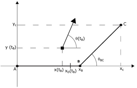
Figure 1.
Trajectory segments switch.
Consider the intervals and , which represent the time frames during which the vehicle traverses the trajectory segments and , respectively. Since these segments are contiguous, the following temporal relationship holds:
At the moment , the vehicle’s position is , and its orientation is . These quantities are expressed in a local reference frame centered at point A, where segment is aligned with the x axis. At , a new local reference frame is established at point B, which is oriented according to . Given that the segment with orientation must be traversed at velocity , the state of (19) at undergoes the following instantaneous update:
where denotes the desired position along segment at time . Refer to Figure 1 for additional details.
Let us thus introduce the following condition:
with being the state of the system at the time instant and being the robust positively invariant region [56] associated with its dynamics. If (4) is held, the sequence of trajectory segments corresponding to arcs and is deemed admissible, enabling the evaluation of another candidate trajectory segment.
2.1. System Model
For trajectory planning purposes, a suitable mathematical description of the dynamics of the vehicle must be used. The modeling solutions that can be found in the literature lie in a trade-off between complexity and descriptivity, ranging from simple kinematic models (which show a good level of accuracy for low-speed cases [17]) to increasingly complex ones, which embed the description of a greater share of physical phenomena [57]. For the purposes of this work, the model presented in [58] was used. The model relies on a few simplifying assumptions, namely, the following:
- The longitudinal forces affecting the tires are due to brakes and engine torque only;
- The considered vehicle uses front-wheel drive, with an equal distribution of torque between front tires, and the braking torque is, instead, evenly distributed among all four tires;
- Tire aligning torques are neglected;
- Dissipative force is made up of drag, rolling friction, and gravity force.
Further assumptions are made in this work:
- The slope is considered as an uncertain parameter;
- The vehicle forward velocity is constant.
Let us introduce the kinematic description of the trajectory tracking. Through some straightforward geometric consideration, the subsequent kinematic model can be formulated to represent the motion of the vehicle:
where , , and define the pose of the vehicle in the inertial reference frame (E), is the longitudinal forward velocity, and the yaw rate is considered positive if it is counterclockwise. For trajectory tracking, Equation (5) is expressed in a local reference frame (L) centered in and oriented with angle see Figure 2.

Figure 2.
Inertial (E) and local (L) reference systems.
Thus, let us define the position of the vehicle in L through the following roto-translation:
where , , and are the pose of center of mass of the vehicle in the local reference frame. Let the desidered pose be , and the let be the nominal forward velocity associated with a trajectory segment; the tracking error in L, centered in and oriented according to the angle , becomes the following:
where , , and .
In [58], the dynamics of the vehicle are described in terms of a nonlinear system whose state vector is the following:
and whose input variables are
i.e., the torque provided by the motor T, the braking force P, and the steering angle , and the road–tire friction coefficient is considered as an unknown but bounded external input:
with , , and being matrices of proper dimensions.
Let be the nominal friction coefficient value and be the torque required to hold the forward speed . Using the classical linearization arguments, the behavior of the system (10) around the nominal condition , , is described by the following linear time-invariant model, which can be written as follows:
with , , and being matrices of proper dimensions.
With being the uniform sampling step, it is possible to obtain the following discrete-time mathematical model:
where , , and . As previously introduced, this work assumes that some elements of the model (12) may be subject to uncertainties. In particular, the mass of the vehicle (which also affects the moment of inertia around the yaw axis) and cornering stiffness of the tires are assumed to fall withing a bounded interval. Such uncertainty can be conveniently embedded in a polytopic mathematical representation [59] through the following convex hull:
with vertices and being its n-th vertex.
2.2. Constrained Control Problem
Let us assume that system (13) must abide by the the following ellipsoidal constraints for state and actuation:
Moreover, let us assume that the following bounds apply to the external disturbance :
The system closed-loop dynamics indeed must take into account the relevant control law which, without loss of generality, is assumed in this work to have the following structure:
It is also assumed that it satisfies, for the system (13), the constraints (14) and (15) and that it guarantees quadratic stability in the positively invariant ellipsoidal region:
which can be found using different procedures, such as the one described in [56].
Thus, taking into account (17), the closed-loop system can be rewritten in the following polytopic form:
being with .
2.3. Trajectory Feasibility
The search for a feasible trajectory for a vehicle with closed-loop dynamics described by (19) and constrained by (14)–(16) can be performed using the methodology developed in [1].
In particular, to address the uncertainties of the model (19), the influence of disturbances (16) and the uncertainty in the initial state , where the set
lets us calculate, following the procedure reported in Appendix A, the set
which accounts for the projection of at time while incorporating the uncertainties in vehicle dynamics (19) and allowable disturbances (16).
For the trajectory segment to follow , the following Minkowski sum condition must hold:
Under this condition, Equation (4) is satisfied regardless of the initial state and for any disturbance . This guarantees the feasibility of transitioning between the two trajectory segments, since it means, in practical terms, that the state of the vehicle will not leave the positively invariant region associated with the constraints. If all trajectory segment sequences meet the admissibility criteria, the entire trajectory is validated as feasible.
Moreover, condition (22) can be reformulated as a Linear Matrix Inequality (LMI) feasibility problem. Specifically, (22) is satisfied if there exists a scalar such that the following LMI is valid:
The proofs are provided in [1].
3. Feasible Trajectory Planning Algorithm
Let the two nodes and represent the starting point S and end point F of a trajectory. A straightforward choice to find (if it exists) the shortest trajectory between them is using the classical algorithm, whose output is a sequence of segments connecting S and F. Such segments are, according to the planning procedure which is used in this work, traversed at a constant forward velocity .
The algorithm employs a heuristic function to evaluate the trajectory linking the initial node to an arbitrary node . This trajectory, denoted by , comprises the sequence of segments connecting S to A at a predefined speed. The length of this trajectory is represented as . Using the notation introduced earlier, the heuristic function is defined as follows:
where represents the Euclidean norm. This function estimates a lower bound on the total length of the path from S to the final node F, incorporating the segments and . Based on (24), the solution to the feasible trajectory planning problem is implemented as a recursive algorithm. The process, starting from the initial node and its associated tracking error , is summarized as follows:
- Identify and evaluate the adjacent node with the most favorable heuristic value relative to ;
- Compute the projection of to the end point of the trajectory segment ;
- If condition (22) is satisfied and A is not the destination node, calculate and repeat the process.
The resulting algorithm is described by the following pseudocode (Algorithm 1).
| Algorithm 1 The pseudocode for the planning algorithm. |
|
It should be noted that only one duplicate node per trajectory is allowed through the flag so that some trajectories, including a loop—which can be useful in practical scenarios—are possible. While the classical algorithm provides an effective foundation for trajectory planning, its heuristic function does not take into account kinodynamic constraints. Its computational complexity in time is, however, in its worst case exponential in the length l (number of nodes) of the shortest path: , with b being the branching factor (i.e., the average number of arcs per node). The heuristics can lower the practical branching factor (i.e., the number of nodes that are actually explored), thus reducing the complexity [60]. Algorithms derived from usually try enhancing the heuristic; among them, the hybrid adds kinematics-related penalty factors. The following section introduces a hybrid algorithm that embeds additional insights into its heuristic function, ensuring both improved efficiency and guaranteed convergence properties by improving the priority in exploring nodes by using properly trained classificators as predictors.
3.1. Artificial Intelligence-Based Heuristic
The algorithm has shown strong performances in solving trajectory problems in systems such as videogames, where the overall state of the machine is not subject to the physical and temporal constraints inherent in nonholonomic systems. While classic A* methods can successfully find optimal trajectories in general cases, these trajectories may be suboptimal or infeasible for applications such as autonomous vehicles. Introducing mechanical constraints requires the penalization or favoring of specific configurations, requiring hybrid systems to compute the cost of individual states differently.
As demonstrated in [50], the algorithm can achieve significant improvements in efficiency by employing an SVM as a heuristic function rather than relying on the standard Euclidean distance heuristic. In this approach, SVMs are utilized to classify different trajectories, defining a nonlinear separation hyperplane that distinguishes acceptable trajectories from nonacceptable ones.
A key advantage of using an SVM as a heuristic in a hybrid lies in the significant reduction of search complexity. Traditional heuristics, such as the Euclidean distance, often require the exploration of thousands of nodes in the search space, leading to increased computational time and complexity. Conversely, when an SVM-based heuristic is applied, the search space can be drastically reduced to fewer nodes, particularly when higher values of (which controls the complexity of the SVM boundary) are used [50]. This reduction occurs because is a hyperparameter that shapes the decision boundary and influences the complexity of the learned model. Specifically, determines the influence of individual data points on the decision boundary according to the following kernel formulation:
The technical advantage of integrating SVMs into the the algorithm lies, in the proposed algorithm, in bypassing the need to check the feasibility of unfeasible trajectories. Instead, the SVM provides a priori decision making for each state, thereby shortening the exploration process, through a soft pruning of the search space.
Beyond the search efficiency gains achieved by employing SVMs, the convergence properties of hybrid algorithms are crucial for ensuring their practical applicability. To this end, this work proposes an improved hybrid A* heuristic function designed to leverage insights from a classificator that has been trained to identify the most promising (in terms of kinodynamic feasibility) trajectory segments, as detailed below. The proposed heuristics are the following:
with and the prediction . The prediction p is the binary output of a properly trained classifier, and its value is 0 if the trajectory segment is classified as nonadmissible, whereas it is 1 if otherwise. The coefficient (whose positiveness ensures the admissibility of the heuristics) is a weight factor that dictates the effect of p: when , p does not affect the order in which adjacent nodes are explored, while moves nodes with to the top of the list of nodes to be explored. The following subparagraphs will focus on the way p is found.
3.2. SVM-Improved Heuristics
The SVM classifier employs a polynomial kernel to classify the eligibility of a trajectory segment stating the nonlinear relationships between three predictors:
- The length of the candidate segment;
- The change in direction;
- The x value in the relevant vector.
The SVM decision function is expressed as
Therein, we have the following:
- is the input feature vector;
- N is the number of support vectors;
- defines the Lagrange multipliers for each support vector;
- defines the class labels of the support vectors, determining whether the input is acceptable or not for a trajectory;
- is the polynomial kernel function;
- b is the bias term.
The sequential minimal optimization (SMO) algorithm is used to solve the convex optimization problem in SVMs due to the nonlinear assumption of the problem. The dual form of the soft-margin SVM is expressed as
It is subject to the following constraints:
where defines the Lagrange multipliers associated with the support vectors, and is the second-order polynomial kernel. SMO iteratively solves two values at a time until meeting its convergence criterion. The misclassification cost is adopted here in the dual form by modifying the bounds of the corresponding Lagrange multipliers by class-specific penalty terms . By assigning different values to different classes, the optimization process penalizes misclassifications of certain classes more than others. This adjustment indirectly modifies the influence of the support vectors and thus the decision boundary during optimization.
3.3. LSTM-Improved Heuristics
The features allowing classification or regression using classical machine learning approaches have the major limitation of being manually designed by developers using a combination of domain expertise and iterative experimentation. Cummins et al. [61] proposed a deep neural network capable of learning optimization heuristics, achieving performance improvements of up to 14% over traditional machine learning approaches. In fact, deep learning can extract information directly from raw data without the need for human experts to label the dataset. It can also use transfer learning to adapt knowledge from one optimization problem to another. A long short-term memory (LSTM) neural network is a deep learning-based approach developed by Hochreiter and Schmidhuber [62]. It is a type of recurrent neural network designed to increase the storage capacity of the network and preserve historical information over subsequent time steps. It is particularly well suited to nonlinear prediction problems and is able to capture temporal dependencies by correlating time series data. A four-layer neural network was designed with a sequence input layer to process the sequential data of three features, followed by a bidirectional LSTM (BiLSTM) recurrent layer that processed the input sequence in both forward and backward directions to capture dependencies in the data over time as follows. The bidirectional LSTM (BiLSTM) layer processes the input sequence in both the forward and backward directions to capture temporal dependencies in the data. The output at each timestep t can be expressed as
Therein, we have the following:
- is the input instance at time step t, where comprises the length of the candidate segment, the change in direction, and the x value in the relevant vector.
- is the weight matrix associated with the input features.
- is the bias term.
- is the output (hidden state) at time t produced by applying the hyperbolic tangent () activation function.
Next, a fully connected layer is used to classify the data into the target classes, while a softmax is used layer to compute class probabilities using a softmax function as follows:
where is the score in terms of the weighted sum of the input features for class c, and j iterates over the two classes (feasible and unfeasible). The LSTM architecture used in this paper is shown in Figure 3.
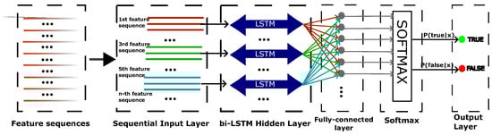
Figure 3.
Schematic of the LSTM architecture.
4. Numerical Results and Discussion
This section illustrates some of the results of a numerical simulation campaign carried out in the MATLAB environment running on an Intel i7-based platform PC. Table 1 lists the relevant parameters that pertain to the simulations. The aim was to carry out a sensitivity analysis against some of the tunable parameters of the proposed architecture.
Section 4.1 describes how the algorithm was trained and the scenario employed. In Section 4.2, we review the algorithm being tested using four different models (model A, B, C, and D) and four couples of destination poses (target A, B, C, and D). The tests in Section 4.3, Section 4.4 and Section 4.5 relied on model A and target A. The subsequent tests did not change neither the destination pose nor the model such that they highlight the effects of a relevant parameter. Namely, in Section 4.3, the effects of the parameter are discussed with tests carried out using the same SVM. In Section 4.4, the effects of the false negative rate and false detection rate are shown while leaving the same accuracy for both classifiers. Finally in Section 4.5, the LSTM-based planning is and its performance is described, discussing the effects of the number of hidden layers in the LSTM.
4.1. Training and Scenario
The planning considered the motion of the vehicle in a 250 m long road segment of a two-lane road that is m wide. Following common procedures in the literature [18,19,20], fixed and moving obstacles (traffic flow) were assumed to be represented by rectangular no-go areas (red boxes in Figure 4). The operational scenario is covered with a grid of 1836 points (graph nodes) and a maximum length of trajectory segments of 10 m, resulting in arcs.

Table 1.
System parameters values (vehicle A is taken from [58]) for tests.
Table 1.
System parameters values (vehicle A is taken from [58]) for tests.
| Parameter | Value | Unit | Uncertainty (%) |
|---|---|---|---|
| Vehicle A | |||
| Vehicle mass | 1550 | kg | 8 |
| Yaw-axis moment of inertia of the vehicle | 1260 | kg/m2 | 10 |
| Rear axle tires stiffness | 43,300 | N/rad | 15 |
| Front axle tires stiffness | 63,700 | N/rad | 15 |
| Forward velocity | 25 | m/s | 10 |
| Vehicle B | |||
| Vehicle mass | 1800 | kg | 8 |
| Yaw-axis moment of inertia of the vehicle | 1500 | kg/m2 | 10 |
| Rear axle tires stiffness | 43,300 | N/rad | 15 |
| Front axle tires stiffness | 63,700 | N/rad | 15 |
| Forward velocity | 20 | m/s | 10 |
| Vehicle C | |||
| Vehicle mass | 1550 | kg | 8 |
| Yaw-axis moment of inertia of the vehicle | 1260 | kg/m2 | 10 |
| Rear axle tires stiffness | 40,000 | N/rad | 15 |
| Front axle tires stiffness | 60,000 | N/rad | 15 |
| Forward velocity | 20 | m/s | 10 |
| Vehicle D | |||
| Vehicle mass | 1300 | kg | 8 |
| Yaw-axis moment of inertia of the vehicle | 1056 | kg/m2 | 10 |
| Rear axle tires stiffness | 43,300 | N/rad | 15 |
| Front axle tires stiffness | 63,700 | N/rad | 15 |
| Forward velocity | 25 | m/s | 10 |
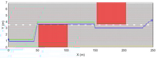
Figure 4.
Two planned trajectories: the SVM-ehnanced one (green line) and the non-SVM-enhanced one (blue line). The trajectories start from the circles on the right. The two red boxes denote two forbidden areas (vehicle A and target A).
The training for the AIs used a dataset consisting of approximately 17,000 instances of the feasible/unfeasible trajectory classes. The dataset was obtained by setting different start and target points with the proper kinds of vehicles and collecting data from the planning procedure using the Euclidean (nonhybrid) . The collected dataset consists of partial trajectories (i.e., the trajectory from the starting point to a candidate segment) in terms of the following:
- The change in pose (angle and tracking error) associated with each segment of the trajectory;
- The length of each trajectory segment;
- The feasible/unfeasible label for the trajectory followed by a candidate segment.
The SVM training was performed considering just the last segment of a partial trajectory, while the LSTM was trained on the whole sequences from the starting point.
It should be noted that uncertainties regarding the vehicle model and road conditions were taken into account by the feasibility check; thus, they were not explicitly changed while creating the dataset, i.e., for a certain vehicle, if a certain uncertain parameter is considered during modeling, the feasibility of a trajectory is guaranteed (and thus it is not influenced) for any allowable value of the parameter in question.
The data were split into 90% for training and 10% for testing for any trained classifier. For the LSTM, the network was trained using the Adam optimizer for a maximum of 200 epochs, with a learning rate of , gradient clipping at a threshold of 1, and the cross-entropy loss function. The data were not shuffled during training, and accuracy was used as the evaluation metric. For the SVM, feature scaling ensured normalization using the mean and standard deviation. The model utilized 64 support vectors to define the decision boundary.
4.2. Algorithm Efficiency
Table 2 shows the number of LMIs solved in a series of tests while varying the vehicle and the target. The baseline used was the classical with Euclidean heuristics, while the tests with used the hybrid heuristics with the SVM classifier. The improvement ranged from roughly (vehicle B/target D) to (vehicle D/target C).
Table 2.
Number of LMI calls varying the vehicle and the target.
4.3. Kf Parameter
Figure 4 shows the results of two plannings with vehicle A and target A. The blue line represents the one performed by setting the parameter to 0, while the green line represents a planning with the parameter set to 1. A further planning with the parameter set to was performed, but it resulted in the same trajectory obtained while considering the . The following results were obtained:
- required the expansion of 181 nodes, with 5430 evaluations of LMIs;
- required the expansion of 174 nodes, with 5394 evaluations of LMIs;
- required the expansion of 174 nodes, with 4003 evaluations of LMIs.
The computational effort related to the classification process was roughly a tenth of the overall computational time, and the workstation used was capable, during tests of running 140,000 classifications per second. Training was carried out in 7 min. The relevant confusion matrix for the SVM used is shown in Figure 5.
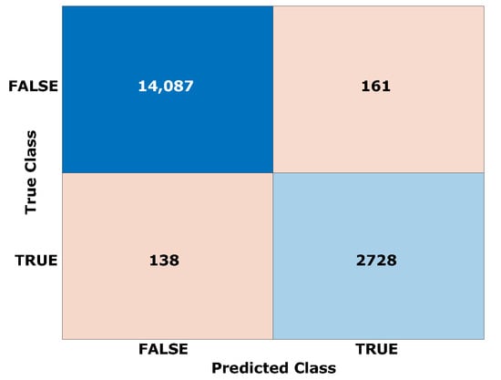
Figure 5.
The confusion matrix of the SVM used, with an accuracy of .
4.4. Training Weights in SVM
A series of tests was carried by training the SVM with different weights matrices of misclassification costs. To isolate the effect of over planning, two matrices were chosen aiming at holding the same accuracy: one lowering the false discovering rate (FDR) at the expense of the false negative rate (FNR) and the other one doing exactly the opposite, which was chosen such that the achieved accuracy would be the same in both cases.
The two confusion matrices are reported in Figure 6. In the first case, the misclassification cost was 0.01 for the true class versus 1 for the false class. In the second case, the misclassification cost was 0.12 for the false class versus 1 for the true class. The measured accuracy came out to and , respectively.
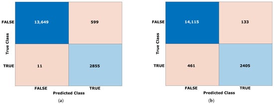
Figure 6.
(a) Confusion matrix for planning with higher FDR. (b) Confusion matrix for planning with higher FNR.
The “higher FDR” case resulted in the benchmark trajectory in the exploration of 182 nodes and the solution of 4389 LMI problems. Conversely, the “higher FNR” case resulted in the exploration of 350 nodes while requiring solving 14,611 LMI; thus, the FNR appears to be the critical parameter in classifier training for trajectory planning.
4.5. Number of LSTM Layers
This subsection shows the tests obtained by considering 40, 5, and 2 hidden layers in the LSTM, with an accuracy of , , and , respectively. The training process took 16, 10, and 8 min, respectively. The process for the 40-layer LSTM is reported in Figure 7, while the two-layer one is reported in Figure 8.
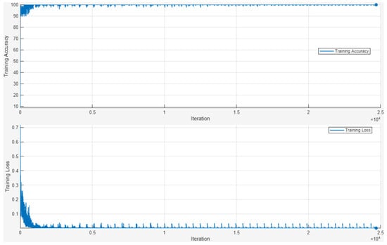
Figure 7.
The training process of the 40-hidden-layer LSTM.
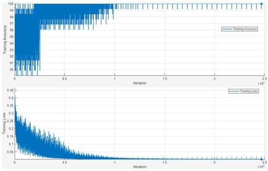
Figure 8.
The training process of the 2-hidden-layer LSTM.
Although the results in terms of expanded nodes were better in terms of both expanded nodes and solved LMIs with respect to the SVM-enhanced planning, the higher computational cost of LSTM-based classification exceeded this benefit. Namely, while the number of node expansions was reduced to 141 and the solved LMIs were 3651, the classification process brought an extra burden of roughly four times more computational effort.
5. Discussion and Conclusions
The scope of this work lies in bringing the formally ensured safety of set-based methods for trajectory planning into artificial intelligence-based ones, with the aim being to exploit the effectiveness of performing the complex tasks that characterize the latter.
By combining a graph-based trajectory planning technique used in robotics with an artificial intelligence-based hybrid , the technique can improve the performance of the baseline set-based method in terms of the time needed to find a first solution (regardless of its optimality) and the time needed to find the optimal solution.
Namely, the SVM-based planning showed up to a 28% reduction in computation effort with respect to the classical “Euclidean” planning (i.e., the planning). Furthermore, it has been shown that higher accuracy is tied with the performance outcomes of the algorithm but also that the false negative rate can significantly hamper the performances.
Furthermore, the possibility to enhance planning through the use of a long-short term memory has been evaluated: although it can improve the efficiency of the algorithm while exploring the environment, its higher computational cost exceeds this benefit. It is interesting to note that the highest accuracy of the LSTM can be reached with just five hidden layers. This result could probably be linked to the fact that the kynodynamic feasibility of a trajectory depends, from a physical point of view, on a part of the trajectory that has been already crossed, and further investigation could exploit this result for improving planning performances.
The results obtained in this work contribute to validating a methodological approach that, while focused on trajectory planning for autonomous vehicles, offers insights and potential for future applications in various scientific and technological contexts. Its possible use in autonomous driving could deal with the local planning of trajectories, not only from the autonomous driving perspective but also in terms of traffic management. In particular, starting from SAE J3016 level 2 features, AVSes require kynodynamically feasible trajectories.
Further deployments will look forward in embedding incremental learning features in the planning framework, without hampering computational efficiency.
Author Contributions
Conceptualization, V.A.N., M.L. and V.S.; Methodology, V.A.N. and M.L.; Software, V.A.N.; Validation, V.A.N.; Formal analysis, V.A.N., F.R. and V.S.; Investigation, V.A.N. and M.L.; Data curation, V.A.N.; Writing—original draft, V.A.N. and M.L.; Writing—review & editing, V.A.N., M.L. and F.R.; Visualization, V.A.N. and F.R.; Supervision, V.S. All authors have read and agreed to the published version of the manuscript.
Funding
This study was partially carried out within the MOST—Sustainable Mobility National Research Center—and received funding from the European Union Next-GenerationEU (PIANO NAZIONALE DI RIPRESA E RESILIENZA (PNRR)—MISSIONE 4 COMPONENTE 2, INVESTIMENTO 1.4—D.D. 1033 17/06/2022, CN00000023). This manuscript only reflects the authors’ views and opinions; neither the European Union nor the European Commission can be considered responsible for them. This work was partially funded by the Next Generation EU Italian NRRP Mission 4, Component 2, Investment 1.5, call for the creation and strengthening of ‘Innovation Ecosystems’, building ‘Territorial R&D Leaders’ (Directorial Decree n. 2021/3277)—project Tech4You—technologies for climate change adaptation and quality of life improvement, n. ECS0000009.
Institutional Review Board Statement
Not applicable.
Informed Consent Statement
Not applicable.
Data Availability Statement
The raw data supporting the conclusions of this article will be made available by the authors on request.
Conflicts of Interest
The authors declare no conflicts of interest.
Appendix A
Let us assume the set (20) of the initial tracking error when the trajectory crosses the point A, and let be its generic instance. At the end of the trajectory segment , each instance will be subject to the following equation:
with and . For each vertex of polytopic linear time invariant system (19) with , it is possible to define the smallest ellipsoidal set
containing all allowable tracking errors at the time instant according to Equation (A1). Such a set can be found by solving the following semi-definite programming minimization problem:
such that
where ,
and is the matrix such that .
Finally, the set the smallest ellipsoidal set
embedding all allowable tracking errors at the time instant can be obtained as the minimum volume ellipsoid containing sets [56].
References
- Scordamaglia, V.; Nardi, V. A Set-Based Trajectory Planning Algorithm for a Network Controlled Skid-Steered Tracked Mobile Robot Subject to Skid and Slip Phenomena. J. Intell. Robot. Syst. 2021, 101, 15. [Google Scholar] [CrossRef]
- Dai, Y.; Xiang, C.; Zhang, Y.; Jiang, Y.; Qu, W.; Zhang, Q. A review of spatial robotic arm trajectory planning. Aerospace 2022, 9, 361. [Google Scholar] [CrossRef]
- Savsani, P.; Jhala, R.L.; Savsani, V.J. Comparative study of different metaheuristics for the trajectory planning of a robotic arm. IEEE Syst. J. 2014, 10, 697–708. [Google Scholar] [CrossRef]
- Ekrem, Ö.; Aksoy, B. Trajectory planning for a 6-axis robotic arm with particle swarm optimization algorithm. Eng. Appl. Artif. Intell. 2023, 122, 106099. [Google Scholar] [CrossRef]
- Zhang, T.; Li, H.; Fang, Y.; Luo, M.; Cao, K. Joint Dispatching and Cooperative Trajectory Planning for Multiple Autonomous Forklifts in a Warehouse: A Search-and-Learning-Based Approach. Electronics 2023, 12, 3820. [Google Scholar] [CrossRef]
- Belter, J.; Hering, M.; Weichbroth, P. Motion Trajectory Prediction in Warehouse Management Systems: A Systematic Literature Review. Appl. Sci. 2023, 13, 9780. [Google Scholar] [CrossRef]
- Morello, R.; De Capua, C.; Lugarà, M.; Lamonaca, F.; Fabbiano, L. Risk model for landslide hazard assessment. IET Sci. Meas. Technol. 2014, 8, 129–134. [Google Scholar] [CrossRef]
- Scholz, S.; Berger, L. Optimization-based Trajectory Planning for Heat Conduction. In Proceedings of the 2024 25th International Carpathian Control Conference (ICCC), Krynica Zdrój, Poland, 22–24 May 2024; pp. 1–5. [Google Scholar]
- Rhein, S.D. Optimal Trajectory Planning for Multiphysics Problems Governed by Electromagnetic and Thermal Phenomena. Ph.D. Thesis, Universität Ulm, Ulm, Germnay, 2018. [Google Scholar]
- Fulco, G.; Ruffa, F.; Lugarà, M.; Filianoti, P.; de Capua, C. Automatic station for monitoring a microgrid. In Proceedings of the 24th IMEKO TC4 International Symposium and 22nd International Workshop on ADC and DAC Modelling and Testing IMEKO TC-4 2020, Palermo, Italy, 14–16 September 2020; pp. 309–314. [Google Scholar]
- Ruffa, F.; Fulco, G.; Lugarà, M.; Filianoti, P.; De Capua, C. A real-time smart charge controller to efficiency charge processes of LiFePO4 batteries. In Proceedings of the 24th IMEKO TC4 International Symposium and 22nd International Workshop on ADC and DAC Modelling and Testing, Palermo, Italy, 14–16 September 2020; pp. 162–167. [Google Scholar]
- Singh, S. Critical Reasons for Crashes Investigated in the National Motor Vehicle Crash Causation Survey; Technical Report; National Center for Statistics and Analysis: Washington, DC, USA, 2015. [Google Scholar]
- Arena, F.; Ticali, D. The development of autonomous driving vehicles in tomorrow’s smart cities mobility. AIP Conf. Proc. 2018, 2040, 140007. [Google Scholar]
- On-Road Automated Driving (ORAD) Committee. Taxonomy and Definitions for Terms Related to Driving Automation Systems for On-Road Motor Vehicles. 2021. Available online: https://doi.org/10.4271/J3016_202104 (accessed on 10 January 2025).
- Kinnear, N.; Stuttard, N.; Hynd, D.; Helman, S.; Edwards, M. Safe Performance of Other Activities in Conditionally Automated Vehicles: Automated Lane Keeping System; Technical Report; UK Department for Transport: London, UK, 2020. [Google Scholar]
- Silvestri, S.; Tricomi, G.; Bassolillo, S.R.; De Benedictis, R.; Ciampi, M. An Urban Intelligence Architecture for Heterogeneous Data and Application Integration, Deployment and Orchestration. Sensors 2024, 24, 2376. [Google Scholar] [CrossRef]
- Paden, B.; Čáp, M.; Yong, S.Z.; Yershov, D.; Frazzoli, E. A survey of motion planning and control techniques for self-driving urban vehicles. IEEE Trans. Intell. Veh. 2016, 1, 33–55. [Google Scholar] [CrossRef]
- Schürmann, B.; Heß, D.; Eilbrecht, J.; Stursberg, O.; Köster, F.; Althoff, M. Ensuring drivability of planned motions using formal methods. In Proceedings of the 2017 IEEE 20th International Conference on Intelligent Transportation Systems (ITSC), Yokohama, Japan, 16–19 October 2017; pp. 1–8. [Google Scholar]
- Burger, C.; Lauer, M. Cooperative multiple vehicle trajectory planning using miqp. In Proceedings of the 2018 21st International Conference on Intelligent Transportation Systems (ITSC), Maui, HI, USA, 4–7 November 2018; pp. 602–607. [Google Scholar]
- Andersen, H.; Alonso-Mora, J.; Eng, Y.H.; Rus, D.; Ang, M.H. Trajectory Optimization and Situational Analysis Framework for Autonomous Overtaking With Visibility Maximization. IEEE Trans. Intell. Veh. 2020, 5, 7–20. [Google Scholar] [CrossRef]
- Pepy, R.; Lambert, A.; Mounier, H. Path planning using a dynamic vehicle model. In Proceedings of the 2006 2nd International Conference on Information & Communication Technologies, Damascus, Syria, 24–28 April 2006; Volume 1, pp. 781–786. [Google Scholar]
- D’Amato, E.; Nardi, V.A.; Notaro, I.; Scordamaglia, V. A Visibility Graph approach for path planning and real-time collision avoidance on maritime unmanned systems. In Proceedings of the 2021 International Workshop on Metrology for the Sea; Learning to Measure Sea Health Parameters (MetroSea), Reggio Calabria, Italy, 4–6 October 2021; pp. 400–405. [Google Scholar] [CrossRef]
- Reif, J.; Sharir, M. Motion planning in the presence of moving obstacles. J. ACM (JACM) 1994, 41, 764–790. [Google Scholar] [CrossRef]
- Claussmann, L.; Revilloud, M.; Gruyer, D.; Glaser, S. A Review of Motion Planning for Highway Autonomous Driving. IEEE Trans. Intell. Transp. Syst. 2020, 21, 1826–1848. [Google Scholar] [CrossRef]
- Villagra, J.; Milanés, V.; Pérez, J.; Godoy, J. Smooth path and speed planning for an automated public transport vehicle. Robot. Auton. Syst. 2012, 60, 252–265. [Google Scholar] [CrossRef]
- Bassolillo, S.; D’Amato, E.; Scapaticci, G.; Blasi, L.; Mattei, M. Ant Colony Algorithm for Path Planning of a Quadrotor UAV. In Proceedings of the Proceedings XXII AIDAA National Congress, Napoli, Italy, 9–12 September 2013. [Google Scholar]
- Bassolillo, S.; Blasi, L.; D’Amato, E.; Mattei, M.; Notaro, I. A recurrent planning strategy for uav optimum path identification in a dynamic environment based on bit-coded flight manoeuvres. In Proceedings of the 2020 International Conference on Unmanned Aircraft Systems (ICUAS), Athens, Greece, 1–4 September 2020; pp. 676–685. [Google Scholar]
- Talamino, J.P.; Sanfeliu, A. Anticipatory kinodynamic motion planner for computing the best path and velocity trajectory in autonomous driving. Robot. Auton. Syst. 2019, 114, 93–105. [Google Scholar] [CrossRef]
- Festl, K.; Stolz, M.; Watzenig, D. Multi-Objective Path Tracking Control for Car-Like Vehicles With Differentially Bounded n-Smooth Output. IEEE Trans. Intell. Transp. Syst. 2024, 25, 8017–8027. [Google Scholar] [CrossRef]
- Kim, J.; Ahn, C. Real-time speed trajectory planning for minimum fuel consumption of a ground vehicle. IEEE Trans. Intell. Transp. Syst. 2019, 21, 2324–2338. [Google Scholar] [CrossRef]
- Elsner, J. Optimizing passenger comfort in cost functions for trajectory planning. arXiv 2018, arXiv:1811.06895. [Google Scholar]
- Typaldos, P.; Papageorgiou, M.; Papamichail, I. Optimization-based path-planning for connected and non-connected automated vehicles. Transp. Res. Part C Emerg. Technol. 2022, 134, 103487. [Google Scholar] [CrossRef]
- Bassolillo, S.R.; Raspaolo, G.; Blasi, L.; D’Amato, E.; Notaro, I. Path Planning for Fixed-Wing Unmanned Aerial Vehicles: An Integrated Approach with Theta* and Clothoids. Drones 2024, 8, 62. [Google Scholar] [CrossRef]
- Bounini, F.; Gingras, D.; Pollart, H.; Gruyer, D. Modified artificial potential field method for online path planning applications. In Proceedings of the 2017 IEEE Intelligent Vehicles Symposium (IV), Los Angeles, CA, USA, 11–14 June 2017; pp. 180–185. [Google Scholar] [CrossRef]
- Boroujeni, Z.; Goehring, D.; Ulbrich, F.; Neumann, D.; Rojas, R. Flexible unit A-star trajectory planning for autonomous vehicles on structured road maps. In Proceedings of the 2017 IEEE International Conference on Vehicular Electronics and Safety (ICVES), Vienna, Austria, 27–28 June 2017; pp. 7–12. [Google Scholar] [CrossRef]
- Fraichard, T. Trajectory planning in a dynamic workspace: A’state-time space’approach. Adv. Robot. 1998, 13, 75–94. [Google Scholar] [CrossRef]
- Kavraki, L.; Svestka, P.; Latombe, J.C.; Overmars, M. Probabilistic roadmaps for path planning in high-dimensional configuration spaces. IEEE Trans. Robot. Autom. 1996, 12, 566–580. [Google Scholar] [CrossRef]
- Qu, P.; Xue, J.; Ma, L.; Ma, C. A constrained VFH algorithm for motion planning of autonomous vehicles. In Proceedings of the 2015 IEEE Intelligent Vehicles Symposium (IV), Seoul, Republic of Korea, 28 June–1 July 2015; pp. 700–705. [Google Scholar] [CrossRef]
- Johnson, J.; Hauser, K. Optimal longitudinal control planning with moving obstacles. In Proceedings of the 2013 IEEE Intelligent Vehicles Symposium (IV), Gold Coast, QLD, Australia, 23–26 June 2013; pp. 605–611. [Google Scholar]
- Liu, C.; Lee, S.; Varnhagen, S.; Tseng, H.E. Path planning for autonomous vehicles using model predictive control. In Proceedings of the 2017 IEEE Intelligent Vehicles Symposium (IV), Los Angeles, CA, USA, 11–14 June 2017; pp. 174–179. [Google Scholar] [CrossRef]
- Wang, Q.; Ayalew, B. Obstacle filtering algorithm for control of an autonomous road vehicle in public highway traffic. In Proceedings of the Dynamic Systems and Control Conference. American Society of Mechanical Engineers, Minneapolis, MN, USA, 12–14 October 2016; Volume 50701, p. V002T24A009. [Google Scholar]
- Pan, H.; Luo, M.; Wang, J.; Huang, T.; Sun, W. A Safe Motion Planning and Reliable Control Framework for Autonomous Vehicles. IEEE Trans. Intell. Veh. 2024, 9, 4780–4793. [Google Scholar] [CrossRef]
- Menon, A.G.; Bindu, S. Artificial intelligence-based trajectory planning for driverless vehicles—A review. In Recent Advances in Hybrid and Electric Automotive Technologies: Select Proceedings of HEAT 2021; Springer: Singapore, 2022; pp. 167–183. [Google Scholar]
- Mir, I.; Gul, F.; Mir, S.; Khan, M.A.; Saeed, N.; Abualigah, L.; Abuhaija, B.; Gandomi, A.H. A Survey of Trajectory Planning Techniques for Autonomous Systems. Electronics 2022, 11, 2801. [Google Scholar] [CrossRef]
- Madridano, Á.; Al-Kaff, A.; Martín, D.; de la Escalera, A. Trajectory planning for multi-robot systems: Methods and applications. Expert Syst. Appl. 2021, 173, 114660. [Google Scholar] [CrossRef]
- Janglova, D. Neural networks in mobile robot motion. Int. J. Adv. Robot. Syst. 2004, 1, 2. [Google Scholar] [CrossRef]
- Claussmann, L.; Carvalho, A.; Schildbach, G. A path planner for autonomous driving on highways using a human mimicry approach with Binary Decision Diagrams. In Proceedings of the 2015 European Control Conference (ECC), Linz, Austria, 15–17 July 2015; pp. 2976–2982. [Google Scholar] [CrossRef]
- Vallon, C.; Ercan, Z.; Carvalho, A.; Borrelli, F. A machine learning approach for personalized autonomous lane change initiation and control. In Proceedings of the 2017 IEEE Intelligent Vehicles Symposium (IV), Los Angeles, CA, USA, 11–14 June 2017; pp. 1590–1595. [Google Scholar] [CrossRef]
- Zhang, P.; Xiong, C.; Li, W.; Du, X.; Zhao, C. Path planning for mobile robot based on modified rapidly exploring random tree method and neural network. Int. J. Adv. Robot. Syst. 2018, 15, 1729881418784221. [Google Scholar] [CrossRef]
- Morsali, M.; Frisk, E.; Åslund, J. Spatio-Temporal Planning in Multi-Vehicle Scenarios for Autonomous Vehicle Using Support Vector Machines. IEEE Trans. Intell. Veh. 2021, 6, 611–621. [Google Scholar] [CrossRef]
- Kim, T.; Lee, H.; Hong, S.; Lee, W. TOAST: Trajectory Optimization and Simultaneous Tracking Using Shared Neural Network Dynamics. IEEE Robot. Autom. Lett. 2022, 7, 9747–9754. [Google Scholar] [CrossRef]
- Bonnavaud, H.; Albore, A.; Rachelson, E. Learning State Reachability as a Graph in Translation Invariant Goal-based Reinforcement Learning Tasks. In Proceedings of the PRL Workshop Series—Bridging the Gap Between AI Planning and Reinforcement Learning, Brussels, Belgium, 14–16 September 2023. [Google Scholar]
- Hafner, D.; Lillicrap, T.; Ba, J.; Norouzi, M. Dream to control: Learning behaviors by latent imagination. arXiv 2019, arXiv:1912.01603. [Google Scholar]
- Wu, Z.; Yu, C.; Chen, C.; Hao, J.; Zhuo, H.H. Plan to predict: Learning an uncertainty-foreseeing model for model-based reinforcement learning. Adv. Neural Inf. Process. Syst. 2022, 35, 15849–15861. [Google Scholar]
- Nardi, V.A. Set-based trajectory planning for a car-like vehicle. In Proceedings of the 2024 10th International Conference on Control, Decision and Information Technologies (CoDIT), Valetta, Malta, 1–4 July 2024; pp. 562–568. [Google Scholar] [CrossRef]
- Boyd, S.; El Ghaoui, L.; Feron, E.; Balakrishnan, V. Linear Matrix Inequalities in System and Control Theory; SIAM: Philadelphia, PA, USA, 1994. [Google Scholar]
- Gillespie, T.D. Fundamentals of Vehicle Dynamics; Technical Report; SAE Technical Paper; SAE: Warrendale, PA, USA, 1992. [Google Scholar]
- Vicente, B.A.H.; James, S.S.; Anderson, S.R. Linear system identification versus physical modeling of lateral–longitudinal vehicle dynamics. IEEE Trans. Control Syst. Technol. 2020, 29, 1380–1387. [Google Scholar] [CrossRef]
- Posthumus-Cloosterman, M. Control over Communication Networks: Modeling, Analysis, and Synthesis. Ph.D. Thesis, Department of Mechanical, Technische Universiteit Eindhoven, Eindhoven, The Nederlands, 2008. [Google Scholar] [CrossRef]
- Pearl, J. Heuristics: Intelligent Search Strategies for Computer Problem Solving; Addison-Wesley Longman Publishing Co., Inc.: Boston, MA, USA, 1984. [Google Scholar]
- Cummins, C.; Petoumenos, P.; Wang, Z.; Leather, H. End-to-End Deep Learning of Optimization Heuristics. In Proceedings of the 2017 26th International Conference on Parallel Architectures and Compilation Techniques (PACT), Portland, OR, USA, 9–13 September 2017; pp. 219–232. [Google Scholar] [CrossRef]
- Hochreiter, S. Long Short-Term Memory; Neural Computation MIT-Press: Cambridge, MA, USA, 1997. [Google Scholar]
Disclaimer/Publisher’s Note: The statements, opinions and data contained in all publications are solely those of the individual author(s) and contributor(s) and not of MDPI and/or the editor(s). MDPI and/or the editor(s) disclaim responsibility for any injury to people or property resulting from any ideas, methods, instructions or products referred to in the content. |
© 2025 by the authors. Licensee MDPI, Basel, Switzerland. This article is an open access article distributed under the terms and conditions of the Creative Commons Attribution (CC BY) license (https://creativecommons.org/licenses/by/4.0/).