Quaternion-Based Fast SMC–PD Cross-Domain Tracking Control for Coaxial Hybrid Aerial–Underwater Vehicle Under Oceanic Disturbances

Abstract

In this study, nonsingular modeling and cross-domain trajectory tracking control problems for a special class of coaxial hybrid aerial–underwater vehicles (HAUVs) are investigated. Coaxial HAUVs need to effectively overcome the influence of hydrodynamic factors when moving underwater, so the attitude angle required by coaxial HAUVs is much larger than that in the air. The attitude representation based on quaternion modeling is adopted to avoid the inherent singularity of Euler angle modeling. A cascade sliding mode control and proportion differentiation (SMC-PD) controller is proposed, which is used to position trajectory and attitude quaternion tracking control, respectively. An adaptive sliding mode controller based on disturbance observer (DO) enhancement is adopted in the outer loop to carry trajectory tracking control. At the same time, the expected attitude angle is calculated by the outer loop (position) and is converted into the expected quaternion. With reference to the idea of enhanced robustness in active disturbance rejection control (ADRC), a feedforward proportion derivation (PD) controller based on DO enhancement is used to track the desired quaternion. A variable parameter adaptive algorithm based on the learning rate is introduced in the cascaded SMC-PD controller. The error convergence speed of the system is further improved by adaptively changing the controller parameters. The stability of the proposed control scheme is proved by using the Lyapunov theory. The numerical simulation results show that the controller has good robustness and effectiveness.

1. Introduction

In recent years, with the development of science and technology and the traction of marine resource exploitation demand, marine robots, such as ocean unmanned aerial vehicles (UAVs) [1], unmanned surface vehicles (USVs) [2], ocean buoys (OBs) [3], and unmanned underwater vehicles (UUVs) [4], have been rapidly developed and achieved great success. This technology is increasingly playing an important role in marine surveillance, offshore rescue, resource exploration, and even military operations. As research results on diverse marine robots continue to emerge, researchers are beginning to think of and design new robots for seemingly impractical amphibious tasks. The hybrid aerial–underwater vehicle (HAUV), which is capable of performing air and water amphibious missions, belongs to a new concept of amphibious vehicles. The concept of amphibious vehicles can even be traced back to the 1930s, when the United States Navy and the Soviet Union, respectively, conceived of flying submarines and underwater aircraft [5] and carried out a series of studies [6,7], but early research was not smooth. After decades of silence, with the progress of marine robotics technology and the increasingly urgent demand for amphibious missions, the development and testing of prototype HAUVs and the pre-research of related technologies have attracted more and more scholars’ research interest.

There are two main ways to implement HAUVs: flying submarines and diving aircraft. At this stage, the most mature scheme mainly refers to existing aviation UAV design schemes, such as fixed-wing structure forms, multi-rotor forms, and bionic design forms [8]. Of course, there are also composite wing HUAVs designed by combining the advantages of various configurations [9,10]. In addition, schemes to realize cross-media motion are mainly divided into fast and slow water surface crossing [10]. The main means of rapid water exiting are compressed gas injection [11] and combustible gas explosion [12,13], while slow water exit processes are mainly achieved with propeller propulsion. In particular, HAUVs with a multi-rotor configuration can achieve vertical take-off and landing (VTOL), which has won the attention of many researchers and achieved many research results. In 2014, the authors of [14] first proposed the double-layer quadrotor configuration HAUV, and the researchers designed a simple proportion derivation (PD) controller for it. Researchers at Rutgers University designed a variable parameter based on a sensor readings proportion integration derivation (PID) controller for their HAUV (Navigator) [15]. At the same time, the team established the attitude model for Navigator by using the quaternion method and successfully carried out high-maneuverability operation testing [16]. In 2019, researchers designed a classical PD flight controller for an HAUV (Loon Copter) equipped with a buoyancy regulation system and successfully achieved take-off and landing on the water surface [17]. For the purpose of further improving the working characteristics of classical linear controllers, the improved PID control strategy is gradually derived. In [18], the researchers proposed an active disturbance rejection control (ADRC) strategy to achieve attitude stability control for a double-layer HAUV and conducted experimental tests near the water. Fuzzy P+ID [19] has also been applied to HAUV systems. In addition, the authors of [20] proposed an improved PID controller, which combines an intelligent genetic algorithm (GA) and radial basis function (RBFNN) to deal with the height control problem of cross-domain processes. The limitation of poor robustness of linear controllers can not be completely overcome by the above improvements. With the progress of control technology, some nonlinear control strategies that have been widely used in quadrotor control have been applied in the HAUV field. For a class of underactuated systems dependent on model parameters, a robust interconnection and damping assignment–passivity-based control (IDA-PBC) strategy was designed [21]. The superiority of the proposed control scheme is verified by the simulation of the quadrotor system with an unknown load. Furthermore, an improved IDA-PBC strategy based on filter observer is proposed to solve the interference and model uncertainty in quadrotor trajectory tracking control. The proposed algorithm can deal with measurement noise and model uncertainty [22]. In particular, sliding mode control (SMC) is widely used in the controller designs of various robot systems due to its insensitivity to model perturbation and strong robustness. The authors of [23] designed a classic SMC controller for a tilting HAUV to verify the effectiveness of the SMC method in altitude and attitude control. Bi et al. [24] designed a second-order SMC controller for a Nezha series multi-rotor. In order to improve the response speed of the control system, the author also designed an adaptive nonsingular fast terminal sliding mode controller for a coaxial HAUV in previous work [25].

Although the above research has fruitfully explored HAUVs to achieve cross-media motion, in practice, the key difficulty is that the additional variables, such as added mass, damping, and the restoring force, change dramatically with the operating state of HAUVs in the trans-medium process. In addition, the combined disturbance of wind and wave load at the water–air interface brings further challenges to the controller design [26]. In [27], it is mentioned that the support arm structure of multi-rotor HAUVs will cause great interference to the dynamics of the vehicle when it breaks through the water surface. Compared to multi-rotor HAUV systems, coaxial HAUV systems have attractive advantages such as a compact structure, excellent hover performance, and so on [28]. Coaxial HAUVs do not require arm structures, which reduces the forward projection area. Therefore, coaxial HAUVs have attracted the interest of researchers in recent years [29,30]. It turns out that this new type of coaxial HAUV has great potential for future development. Inspired by the above research and referring to existing coaxial aircraft, the author developed a coaxial HAUV system in [25]. 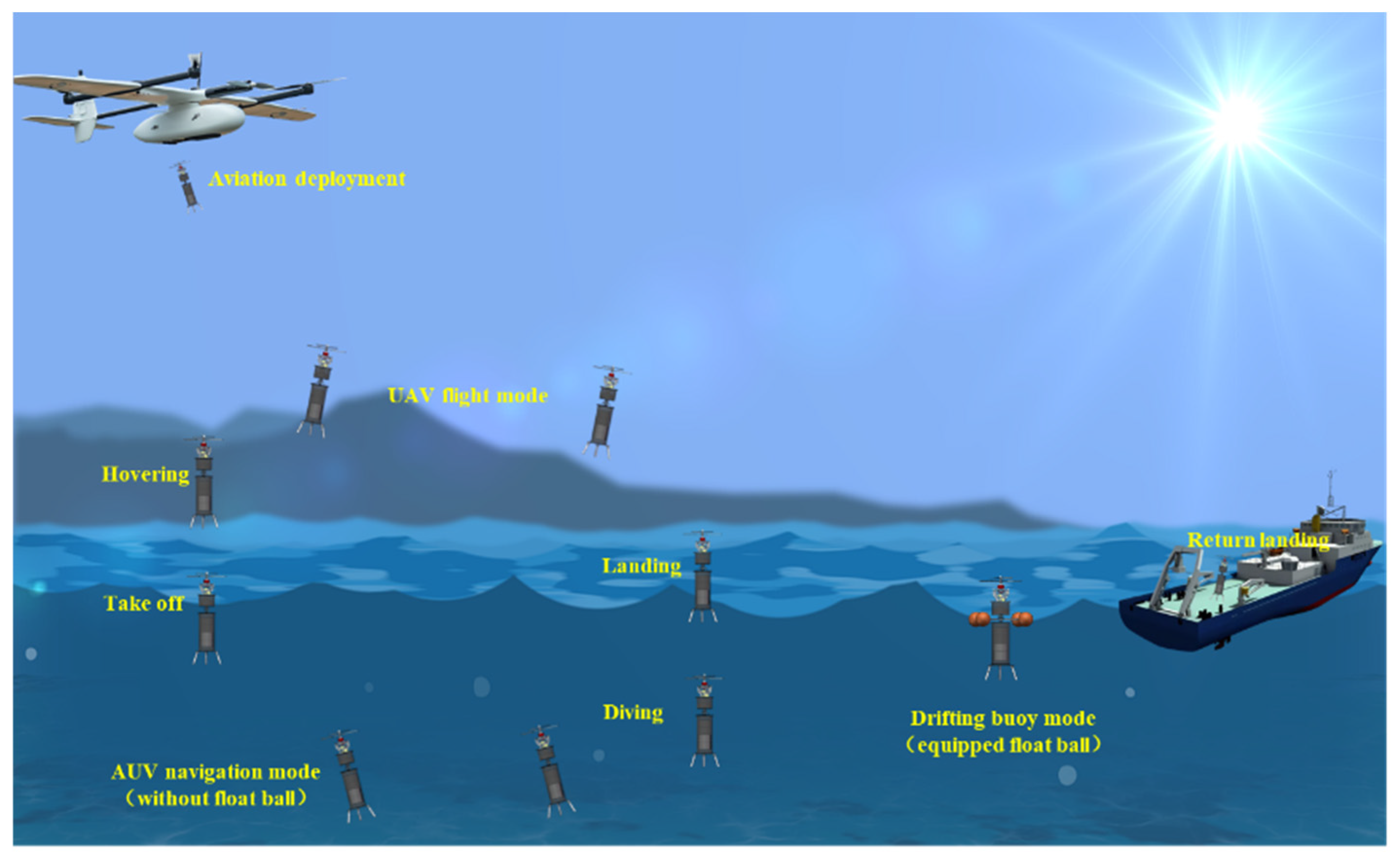Figure 1 shows the operation flow chart of the designed coaxial HAUV. As can be seen in Figure 1, coaxial HAUV can use two operating modes according to different tasks.

In the initial phase of controller design, the mathematical model of an HAUV should be established first. However, most existing HAUVs mainly adopt the modeling idea of quadrotor UAV, that is, modeling based on the small-angle assumption. This limits the model description of HAUV in the large-angle state. Mainstream methods for describing attitude parameters include the rotation matrix, Euler angle, Rodriguez parameters (RPs), modified Rodriguez parameters (MRPs), quaternion, etc. [4]. Because it is relatively easy to understand in terms of physical interpretation, most UUV and UAV control schemes are based on the Euler angle representation for attitude control. However, the use of the Euler angle to represent the attitude may cause a singularity when the vehicle approaches a singular direction. In most UAV and AUV scenarios, this is usually not a serious problem, as the vehicle only needs to operate at angles close to the equilibrium point and away from the singularity [31]. For the sake of effectively overcoming the large drag, the propulsion force needs to be more distributed in the forward direction, which requires a large inclination angle. To study the stability of HAUVs under a large angle of inclination under harsh sea conditions, it is a valuable option to choose the attitude resolution method based on quaternion representation [32]. The quaternion unit has been widely used in spacecraft attitude control or satellite attitude control [33,34], but spacecraft attitude control does not consider translational motion. Both translational and rotational motion should be considered for the trans-medium motion control problem of HAUVs. Therefore, these control schemes cannot be directly applied to the motion control of HAUVs. In [35], the quaternion-based PD attitude control method was applied to the motion control of a six-degrees of freedom (DOF) AUV, but it lacks measures to further enhance its robustness. In [16], the PD algorithm based on quaternion is also adopted in the attitude control of HAUV. This solves the problem of large-angle maneuvering but also lacks sufficient consideration of the robustness of the controller.

Motivated by the above discussion, an appropriate strategy must be proposed to solve this singular constraint to improve HAUV mobility. According to the underactuated characteristics of a coaxial HAUV system, it was divided into inner (attitude) and outer (position) loops [36], and controllers were designed, respectively. In the outer loop trajectory tracking control loop, the adaptive sliding mode control (ASMC) technology enhanced by disturbance observer (DO) [37] was used to calculate the thrust and the expected attitude angle. The disturbance observer was combined with an adaptive technique to compensate for the lumped uncertainty, which effectively weakens the inherent chattering phenomenon of sliding mode control. The calculated attitude angle was converted into a desired quaternion, and a DO-enhanced robust feedforward PD control algorithm was used to track the target quaternion. Finally, a variable parameter design scheme based on the learning rate was introduced into the cascaded SMC-PD controller, and the error convergence speed of the system was further improved by adaptively changing the controller parameters [38]. In order to realize fast and stable cross-domain tracking control of coaxial HAUV systems, a DO-based SMC-PD control strategy is proposed in this paper. The contributions of this paper are as follows:

(1)

Removing the limitation of the small-angle assumption, a six-DOF cross-domain dynamic model that can perform large-angle maneuvering is established. The quaternion attitude modeling scheme is adopted to avoid the singularity problem of HAUV.

(2)

In the hierarchical cascade SMC-PD controller, the control gain parameters are adaptively changed by using the learning rate method, which improves the error convergence speed of the system.

(3)

A DO with a simple structure is adopted to supplement the uncertainty in the dynamic model and enhance the robustness of the system.

The arrangement of the rest of this manuscript is outlined as follows: in Section 2, the dynamics model of the cross-domain process of a coaxial HAUV is analyzed and established. The attitude dynamics model based on quaternion representation is introduced. In Section 3, the design process of the control strategy is given, and the stability of the proposed control scheme is proved by using the Lyapunov theory. The control performance of the designed controller is analyzed by using the numerical simulation study in Section 4. Finally, Section 5 presents some conclusions and perspectives as well as an outlook for future work.

2. Dynamic Modeling

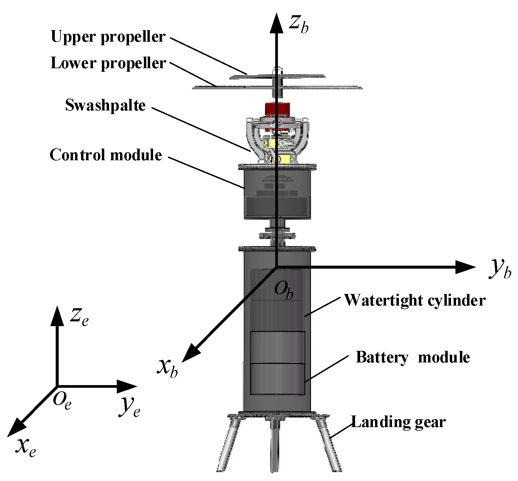
In this paper, the studied object is the coaxial HAUV, as shown in Figure 2. In order to accurately describe the motion of the vehicle and the dynamics model, two coordinate systems should be given first: the inertial coordinate system $R_E\left\{O_e{x}_e{y}_e{z}_e\right\}$ and the body-fixed coordinate system $R_B\left\{O_b{x}_b{y}_b{z}_b\right\}$ will be defined. The origin of the body-fixed coordinate system is set at the position of the heavy center of the vehicle. The inertial co-ordinate system is fixed at sea level, plane $x_e{O}_e{y}_e$ coincides with a calm water surface, and $O_e{z}_e$ points in the direction of the sky. The position and linear velocity vector of the HAUV are defined as ${\eta }_1={\left[\begin{array}{ccc}x& y& z\end{array}\right]}^{\mathrm{T}}$, ${\nu }_1={\left[\begin{array}{ccc}u& v& w\end{array}\right]}^{\mathrm{T}}$, and the attitude angle and angular velocity of the vehicle are denoted as ${\eta }_2={\left[\begin{array}{ccc}\varphi & \theta & \psi \end{array}\right]}^{\mathrm{T}}$, $\omega ={\left[\begin{array}{ccc}p& q& r\end{array}\right]}^{\mathrm{T}}$.

Here, $J$ is the transformation matrix from the body coordinate system to the inertial coordinate system.

The kinematic equation of the coaxial HAUV is expressed as follows:

$$\dot{\eta }=J\nu$$

(1)

The meanings of each variable and symbol in the equation are as follows:

$$\begin{array}{c}\eta ={\left[\begin{array}{cc}{\eta }_1^{\mathrm{T}}& {\eta }_2^{\mathrm{T}}\end{array}\right]}^{\mathrm{T}},\nu ={\left[\begin{array}{cc}{\nu }_1^{\mathrm{T}}& {\omega }^{\mathrm{T}}\end{array}\right]}^{\mathrm{T}},J=\left[\begin{array}{cc}{J}_1& 0^{3\times 3}\\ 0^{3\times 3}& J_2\end{array}\right],\\ J_1=\left[\begin{array}{ccc}\cos \theta \cos \psi & \sin \varphi \sin \theta \cos \psi -\cos \varphi \sin \psi & \cos \varphi \sin \theta \cos \psi +\sin \varphi s\mathrm{in}\psi \\ \cos \theta \sin \psi & \sin \varphi \sin \theta \sin \psi +\cos \varphi \cos \psi & \cos \varphi \sin \theta \sin \psi -\sin \varphi \cos \psi \\ -\sin \theta & \sin \varphi \cos \theta & \cos \varphi \cos \theta \end{array}\right],\\ J_2=\left[\begin{array}{ccc}1& \sin \varphi \tan \theta & \cos \varphi \tan \theta \\ 0& \cos \varphi & -\sin \varphi \\ 0& \sin \varphi /\cos \theta & \cos \varphi /\cos \theta \end{array}\right]\end{array}$$

Assumption 1.

To facilitate the controller design, we simplify the HAUV model and make the following basic assumption. The main mass of the HAUV is uniformly distributed on the cylindrically shaped watertight hull, and its geometric structure is symmetric about three coordinate planes. High-order hydrodynamic coefficients will not be considered.

Since the main structure of the HAUV is uniform, it can be approximately considered that variables such as additional mass, buoyancy, and drag are linearly related to the height of the submerged part of the vehicle [23,39]. Therefore, a switching coefficient is adopted to approximate the change trend of additional variables in the trans-medium process in the trans-medium stage. The existing switching coefficients mainly have a step form $k_{sn}$ [14] and a linearized form $k_{ln}$ [25,39]. The two switching functions are discontinuous and easily cause controller instability. This paper proposes a switching function, $k_{th}$, based on the hyperbolic tangent function, which makes the model switching smoother and more stable.

$$\begin{array}{l}{k}_{ln}=\left\{\begin{array}{c}0,z\ge h/2\\ 1/2\left(1-2z/h\right),-h/2<z<h/2\\ 1,z\le -h/2\end{array}\right.\\ k_{sn}=1/2\left(1-\mathrm{sign}\left(z\right)\right)\\ k_{th}=1/2\left(1-\tanh \left(z/\mu \right)\right)\end{array}$$

(2)

where $h$ is the altitude of the vehicle, $z$ represents the height value of the vehicle in the inertial coordinate system, and $0<\mu <1$ is the parameter to be designed. $k_s=k_{tanh}$ represents the approximate change in the hydrodynamics in the transmedia process; $k_{sa}=1-k_s$ indicates the switching coefficient of the aerodynamics, which describes the trend of the influencing factors in the air.

Next, the cross-media dynamic evolution process of parameters and variables in the model will be analyzed.

2.1. Added Mass

Considering the approximate symmetry of the HAUV, the mass matrix and moment of inertia matrix are both main diagonal matrices [23,24], which can be expressed as follows:

$$M=M_{RB}+M_A$$

(3)

where $M=M_{RB}+M_A$ is the mass matrix, $M_{RB}=\mathrm{diag}\left(m,m,m,I_x,I_y,I_z\right)$ and $M_A$ are the nominal (when the body is drying) mass matrix and additional mass matrix, respectively. A coaxial HAUV will carry a part of the water (near its body) with it during underwater maneuvering, which is the cause of additional mass. The added mass matrix can be approximated in the form of a principal diagonal matrix, $M_A=-k_{s}diag\left(X_{\dot{u}},Y_{\dot{v}},Z_{\dot{w}},K_{\dot{p}},M_{\dot{q}},N_{\dot{r}}\right)$. $M$ is a diagonal matrix, which can be expressed as a partitioned matrix $M=\left[\begin{array}{cc}{M}_{11}& 0_{3\times 3}\\ 0_{3\times 3}& M_{22}\end{array}\right]$.

2.2. Coriolis Force

The Coriolis force comes from the inertia of an object’s motion. From the definition of the Coriolis force, it can be seen that this is an inherent property of moving objects. The Coriolis force is also time-varying, which can be expressed as follows:

$$C_v=C_{RB}+C_A$$

(4)

$$\begin{array}{l}{C}_{RB}=\left[\begin{array}{cccccc}0& 0& 0& 0& mw& -mv\\ 0& 0& 0& -mw& 0& mu\\ 0& 0& 0& mv& -mu& 0\\ 0& mw& -mv& 0& I_{z}r& -I_{y}q\\ -mw& 0& mu& -I_{z}r& 0& I_{x}p\\ mv& -mu& 0& I_{y}q& -I_{x}p& 0\end{array}\right]\\ C_A\left.=\left[\begin{array}{cccccc}0& 0& 0& 0& -Z_{\dot{w}W}& Y_{\dot{v}V}\\ 0& 0& 0& Z_{\dot{w}W}& 0& -X_{\dot{u}U}\\ 0& 0& 0& -Y_{\dot{v}V}& X_{\dot{u}}u& 0\\ 0& -Z_{\dot{w}W}& Y_{\dot{v}V}& 0& -N_{\dot{r}}r& M_{\dot{q}}q\\ Z_{\dot{w}W}& 0& -X_{\dot{u}}u& N_{\dot{r}}r& 0& -K_{\dot{p}}p\\ -Y_{\dot{v}V}& X_{\dot{u}}u& 0& -M_{\dot{q}}q& K_{\dot{p}}p& 0\end{array}\right.\right]\end{array}$$

(5)

where $C_v$ represents Coriolis matrices, and $C_{RB}$ and $C_A$ are the nominal and additional Coriolis force matrices, respectively. Obviously, matrix $C_A$ is related to the added mass of the HAUV and the current motion state, and when the added mass disappears, $C_A$ also returns to 0.

2.3. Resistance and Moment of Resistance

Drag and torque are generally considered to be proportional to the square of the linear and angular velocities of underwater (aerial) motion [40].

$$\left[\begin{array}{l}{f}_d\\ {\tau }_d\end{array}\right]=-D({\nu }_1,{\nu }_2)\left[\begin{array}{l}{\nu }_1\\ {\nu }_2\end{array}\right]$$

(6)

$$\begin{array}{cc}{D}_v& =D_w+D_a\\ & =k_{s}diag\left(X_{u|u|}\left|u\right|,Y_{v|v|}\left|v\right|,Z_{w|w|}\left|w\right|,K_{p|p|}\left|p\right|,M_{q|q|}\left|q\right|,N_{r|r|}\left|r\right|\right)\\ & +k_{sa}diag\left(X_{u|u|a}\left|u\right|,Y_{v|v|a}\left|v\right|,Z_{w|w|a}\left|w\right|,\left.K_{p|p|a}\left|p\right|,M_{q|q|a}\left|q\right|,N_{r|r|a}\left|r\right|\right]\right)\end{array}$$

(7)

Here, $D_w$ and $D_a$ are the drag coefficient matrices of the coaxial HAUV in water and air, respectively; $D$ is the combined drag coefficient.

2.4. Restoring Force and Restoring Moment

In the inertial coordinate system, the direction of the HAUV subjected to gravity in the water is opposite to the positive direction of the axis, but the direction of buoyancy is the same as the positive direction of the axis. Buoyancy is obtained by using Archimedes’ principle, where gravity and buoyancy are, respectively, as follows:

$$\begin{array}{cc}{f}_g& =-mg{J}_1^T{\left[\begin{array}{ccc}0& 0& 1\end{array}\right]}^T\\ & =-mg{\left[\begin{array}{ccc}-\sin \theta & \sin \varphi \cos \theta & \cos \varphi \cos \theta \end{array}\right]}^T\\ {\tau }_g& ={[\begin{array}{ccc}0& 0& 0\end{array}]}^T\end{array}$$

(8)

$$\begin{array}{cc}{f}_b& =k_s{\rho }_{w}Vg{J}_1^T{\left[\begin{array}{ccc}0& 0& 1\end{array}\right]}^T\\ & =k_s{\rho }_{w}Vg{\left[\begin{array}{ccc}-\sin \theta & \sin \varphi \cos \theta & \cos \varphi \cos \theta \end{array}\right]}^T\\ {\tau }_b& =r_b\times f_b\end{array}$$

(9)

Here, ${\rho }_w$, $V$, and $g$ are defined as the density of water, the volume of the HAUV watertight chamber, and the gravitational acceleration, respectively. Since the origin of the coordinate system is chosen to be located at the center of gravity of the HAUV, no torque is generated by gravity. The center of buoyancy is $r_b={\left[\begin{array}{ccc}{x}_b& y_b& z_b\end{array}\right]}^{\mathrm{T}}$. Based on the above analysis, the restoring force is expressed as a vector:

$$g_{\nu }=-\left[\begin{array}{l}{f}_g+f_b\\ {\tau }_g+{\tau }_b\end{array}\right]$$

(10)

Remark 1.

It is worth noting that, according to the basics of ship principles, the stability of a floating body is closely related to the relative position of the center of buoyancy to the center of gravity, which changes dynamically. The special elongated structure of the coaxial HAUV leads to a minimal change in the horizontal position of the center of buoyancy during its trans-domain motion. The simplified rule of change in the vertical position of the center of action of the wind force and the center of buoyancy is given here:

$$\begin{array}{l}{z}_b=\left\{\begin{array}{c}0,z>h/2\\ k_s{z}_{b0}-\left(h/2+z\right)/2,-h/2\le z\le h/2\\ z_{b0},z<-h/2\end{array}\right.\\ z_w=\left\{\begin{array}{c}0,z>h/2\\ h/2-\left(h/2+z\right)/2,-h/2\le z\le h/2\\ 0,z<-h/2\end{array}\right.\end{array}$$

(11)

where $z_{b0}$ is the vertical coordinate value of the center of buoyancy in the body-fixed coordinate system under fully submerged HAUV conditions.

The position of the center of action of the wind force and the center of buoyancy in the body-fixed coordinate system can be approximated by using mathematical calculations.

$$\begin{array}{l}{r}_b={\left[\begin{array}{ccc}{z}_b\sin (\theta )& -z_b\sin (\varphi )& z_b\end{array}\right]}^{\mathrm{T}}\\ r_w={\left[\begin{array}{ccc}-z_w\sin (\theta )& z_w\sin (\varphi )& z_w\end{array}\right]}^{\mathrm{T}}\end{array}$$

(12)

2.5. Control Forces and Moments

The two propellers of the coaxial HAUV are fixed on the vector tilting device, and the vector platform controls the output of force and torque by controlling the tilt angle. The control force and torque generated by them can be expressed as follows [36,41]:

$$T=\left[\begin{array}{c}{T}_x\\ T_y\\ T_z\end{array}\right]=R\left({\delta }_x,{\delta }_y\right)\left[\begin{array}{c}0\\ 0\\ k_{\alpha }{\omega }_1^2+\sigma k_{\beta }{\omega }_2^2\end{array}\right]$$

(13)

$$R\left({\delta }_x,{\delta }_y\right)=\left[\begin{array}{ccc}\cos {\delta }_y& -\sin {\delta }_y\sin {\delta }_x& -\sin {\delta }_y\cos {\delta }_x\\ 0& \cos {\delta }_x& -\sin {\delta }_x\\ \sin {\delta }_y& \cos {\delta }_y\sin {\delta }_y& \cos {\delta }_x\cos {\delta }_y\end{array}\right]$$

(14)

$${\tau }_{\mathrm{\Theta }}=\left[\begin{array}{c}{u}_2\\ u_3\\ u_4\end{array}\right]=\left[\begin{array}{c}-d\sin {\delta }_x\left(k_{\alpha }{\omega }_1^2+\sigma k_{\beta }{\omega }_2^2\right)\\ -d\sin {\delta }_y\cos {\delta }_x\left(k_{\alpha }{\omega }_1^2+\sigma k_{\beta }{\omega }_2^2\right)\\ {\gamma }_{\alpha }{\omega }_1^2+{\gamma }_{\beta }{\omega }_2^2\end{array}\right]$$

(15)

where $k_{\alpha }$ and $k_{\beta }$ are the lift coefficients of the upper and lower propellers, respectively, $\sigma$ is the lift loss coefficient of the lower propeller, and $d$ is the distance from the lift center of the propeller to the center of mass. $R\left({\delta }_x,{\delta }_y\right)$ represents the mapping transformation matrix from the propeller thrust to body coordinate system; ${\delta }_x$ and ${\delta }_y$ represent the deflection angle of the vector tilt device.

Remark 2

 ([41,42]). From a practical flight control point of view, considering that the tilting platform angles are all small, we can obtain $\cos {\delta }_x\approx 1$, $\cos {\delta }_y\approx 1$, $\sin {\delta }_x\approx {\delta }_x\approx 0$, and $\sin {\delta }_y\approx {\delta }_y\approx 0$. The control model can be simplified, where $T_x$ and $T_y$ are very small compared to each other, $T_z$, and the effect of this and can be ignored. For convenience of presentation, $T_z$ is redefined as $u_1$.

The control force generated in the body coordinate system is rewritten as

$${\tau }_{\nu }={\left[\begin{array}{cc}{\tau }_{vp}^{\mathrm{T}}& {\tau }_{v\mathrm{\Theta }}^{\mathrm{T}}\end{array}\right]}^{\mathrm{T}}={\left[\begin{array}{cccccc}0& 0& u_1& u_2& u_3& u_4\end{array}\right]}^{\mathrm{T}}$$

(16)

Remark 3.

${\tau }_{vp}$ and ${\tau }_{v\mathrm{\Theta }}$ are the actual control inputs of the position subsystem and attitude subsystem, respectively. It is obvious that the position subsystem has only one control input to control the 3-DOF translational motion, which is a typical underdriven system.

2.6. Analysis of the Interference Mathematical Model

In this section, the interference of wind, waves, and currents is reasonably modeled, and the proposed interference mathematical model is used to simulate the external environment, which makes the simulation experiment closer to the actual situation.

2.6.1. Sea Breeze Interference

Sea breeze disturbances can be divided into average (steady) wind disturbances and pulsating wind disturbances. The equation of additional disturbance force, $F_{wind}$, and torque, $M_{wind}$, caused by average wind disturbance to the HAUV is as follows [40,43]:

$$\left\{\begin{array}{l}{F}_{wind}=-C_{dw}\left|v_{rw}\right|v_{rw}\\ M_{wind}=r_w\times F_{wind}\end{array}\right.$$

(17)

Assuming that the constant wind has a constant inertial reference speed,

$v_w\in R^3$, the relative speed of the HAUV moving in the wind is $v_{rw}=v-v_w$; the geometric center of the HAUV body exposed to the air is the center of the wind pressure, and its position in the vehicle body is denoted by $r_w\in R^3$; $C_{dw}$ represents the wind damping coefficient.

2.6.2. Ocean Current Interference

The influence of ocean currents is similar to the influence of sea wind, and its magnitude is proportional to the square of the relative velocity. The force $F_c$ and moment $M_c$ generated by ocean currents can be expressed by the following expression:

$$\left\{\begin{array}{l}{F}_c=-C_{dc}\left|v_{rc}\right|v_{rc}\\ M_c=r_b\times f_c\end{array}\right.$$

(18)

In the simulation, the ocean current is generally considered constant and uniform, and it is assumed that the ocean current has a constant inertial reference velocity, $v_c\in R^3$; $v_{rc}=v-v_c$ is the relative velocity of the HAUV in the ocean current, and $C_{dc}$ represents the water damping coefficient.

2.6.3. Wave Interference

In order to simplify the problem, wave interference caused by single-frequency micro-amplitude-long peak waves with a fixed direction is considered [40,44]. It is assumed that these waves are regular waves concentrated in the x-axis and y-axis directions.

The corresponding velocity potential functions ${\Gamma }_x$ and ${\Gamma }_y$ re expressed as

$$\begin{array}{l}{\Gamma }_x={\displaystyle \sum _{i=1}^N}{\displaystyle \frac{g{A}_{xi}}{{\omega }_{xi}}}{e}^{k_{xi}z}\sin (k_{xi}x-{\omega }_{xi}t+{\phi }_{xi})\\ {\Gamma }_y={\displaystyle \sum _{i=1}^N}{\displaystyle \frac{g{A}_{yi}}{{\omega }_{yi}}}{e}^{k_{yi}z}\sin (k_{yi}y-{\omega }_{yi}t+{\phi }_{yi})\end{array}$$

(19)

where $N$, $A_{ji}$, ${\omega }_{ji}$, $k_{ji}$, and ${\phi }_{ji}$($j=x,y$) are the total number of waves, wave amplitude, wave frequency, wave number, and wave phase, respectively. A simple dispersion relation is satisfied between the wave number and the circular frequency of a wave, i.e., $k_{ji}=w_{ji}^2/g$.

The transverse and vertical velocities of the wave in the x- and y-axis directions and the corresponding accelerations are given by the following equation:

$$\begin{array}{l}{u}_x={\displaystyle \frac{\partial {\Gamma }_x}{\partial x}},w_x={\displaystyle \frac{\partial {\Gamma }_x}{\partial z}},u_y={\displaystyle \frac{\partial {\Gamma }_y}{\partial y}},w_y={\displaystyle \frac{\partial {\Gamma }_y}{\partial z}}\\ {\dot{u}}_x={\displaystyle \frac{\partial u_x}{\partial t}},{\dot{w}}_x={\displaystyle \frac{\partial w_x}{\partial t}},{\dot{u}}_y={\displaystyle \frac{\partial u_y}{\partial t}},{\dot{w}}_y={\displaystyle \frac{\partial w_y}{\partial t}}\end{array}$$

(20)

The effect of the HAUV on the incident wave pressure field can be neglected. Therefore, the wave loads encountered by the vehicle at the water surface can be calculated according to the following equation [24]

$$\begin{array}{l}{F}_{wave,x}={{\displaystyle \int }}_{L_z}({\rho }_w{C}_m\pi R^2{\dot{u}}_x+{\displaystyle \frac{1}{2}}{\rho }_w{C}_{d}R{u}_x|u_x|)dz\\ F_{wave,y}={{\displaystyle \int }}_{L_z}({\rho }_w{C}_m\pi R^2{\dot{u}}_y+{\displaystyle \frac{1}{2}}{\rho }_w{C}_{d}R{u}_y|u_y|)dz\\ M_{wave}=r_b\times F_{wave}\\ F_{wave}=J_1^T{\left[F_{wave,x},F_{wave,y},0\right]}^T\end{array}$$

(21)

where $R$ is the body radius of the coaxial HAUV and $C_m$ and $C_d$ are the inertia and drag coefficients of the watertight hull of the coaxial HAUV, respectively. $L_z$ denotes the integral length of the cabin subjected to wave action, which is expressed as

$$L_z\in \left\{\begin{array}{l}\left[0,0\right],z\ge H/2\\ \left[z-H/2,0\right],-H/2<z<H/2\\ \left[z-H/2,z+H/2\right],z\le H/2\end{array}\right.$$

(22)

where $H$ is the body height of the coaxial HAUV, and $z$ is the value of the altitude in the inertial frame.

The above marine environmental parameters applied in the simulation are detailed in Appendix A,

Table A1. Wind, wave, and current simulation parameters.

Parameter Symbol	Value	Parameter Symbol	Value
$A_{x1}/\mathrm{m}$	0.1	$A_{y1}/\mathrm{m}$	0.07
$A_{x2}/\mathrm{m}$	0.03	$A_{y1}/\mathrm{m}$	0.04
${\omega }_{x1}/\left(rad\cdot {\mathrm{s}}^{-1}\right)$	1	${\phi }_{x1}/\mathrm{rad}$	0
${\omega }_{x2}/\left(rad\cdot {\mathrm{s}}^{-1}\right)$	10	${\phi }_{x2}/\mathrm{rad}$	0
${\omega }_{y1}/\left(rad\cdot {\mathrm{s}}^{-1}\right)$	2	${\phi }_{y1}/\mathrm{rad}$	0
${\omega }_{y2}/\left(rad\cdot {\mathrm{s}}^{-1}\right)$	7	${\phi }_{y2}/\mathrm{rad}$	0
$C_{dw}/\left(\mathrm{N}\cdot {\mathrm{m}}^{-2}\cdot {\mathrm{s}}^2\right)$	0.1	$C_m$	0.8
$C_{dc}/\left(\mathrm{N}\cdot {\mathrm{m}}^{-2}\cdot {\mathrm{s}}^2\right)$	0.03	$C_D$	0.8
$v_w/\left(\mathrm{m}\cdot {\mathrm{s}}^{-1}\right)$	(0.1,0.1,0)	$v_c/\left(\mathrm{m}\cdot {\mathrm{s}}^{-1}\right)$	(−0.1,−0.1,0)

.

Remark 4.

Based on the detailed analysis of the various external forces and moments applied to the system in the previous subsection, they can be classified. The first category is the active control forces that need to be regulated by the controller, i.e., control forces and control moments, ${\tau }_v$; the second category consists of external forces that can be measured or approximated, such as the Coriolis forces matrix, $C_v$, restoring forces, $g_v$, damping matrix,, etc.; and the third category consists of terms that are not practically measurable or are extremely expensive to model accurately, such as wind-disturbing forces ($F_{wind}$, $M_{wind}$), wave-disturbing forces ($F_{wave}$, $M_{wave}$), current-disturbing forces ($F_c$, $M_c$), and so on. The third type of external forces can be approximated using empirical equations, but it is very difficult to obtain real-time information about the marine environment, which has limited accuracy.

2.7. Dynamic Modeling of Coaxial HAUV

Referring to the relevant experience with underwater robots, the coaxial HAUV dynamics can be expressed in Newton–Euler equation form as

$$\left\{\begin{array}{l}\dot{\eta }=J\nu \\ M\dot{\nu }+C_{\nu }\nu +D_{\nu }\nu +g_{\nu }={\tau }_{\nu }+{\tau }_d\end{array}\right.$$

(23)

where ${\tau }_d={\left[\begin{array}{cc}{d}_p^{\mathrm{T}}& d_{\mathrm{\Theta }}^{\mathrm{T}}\end{array}\right]}^{\mathrm{T}}$ is lumped uncertainty, which includes modeling uncertainty, model approximation error, and generalized external disturbance.

To simplify the presentation, referring to the relevant experience with underwater robots, the above model (23) is translated into an inertial coordinate system [45]:

$$M_{\eta }\ddot{\eta }+C_{\eta }\dot{\eta }+D_{\eta }\dot{\eta }+g_{\eta }={\tau }_{\eta }+{\tau }_{d\eta }$$

(24)

where the transformed variables satisfy the following relationship: $M_{\eta }=J^{-\mathrm{T}}M{J}^{-1}$, $C_{\eta }=J^{-\mathrm{T}}\left(C-M{J}^{-1}\dot{J}\right)J^{-1}$, $D_{\eta }=J^{-\mathrm{T}}D{J}^{-1}$, $g_{\eta }=J^{-\mathrm{T}}{g}_{\nu }$, ${\tau }_{d\eta }=J^{-\mathrm{T}}{\tau }_{d\nu }$.

In order to facilitate the subsequent controller design, the translational motion and the rotational motion in the dynamic model of Equation (24) are separated into two subsystems, as shown in Equation (25):

$$\begin{array}{l}\mathrm{A}:\left\{\begin{array}{l}{\dot{\eta }}_1=v_{1I}\\ {\dot{v}}_{1I}={\tau }_p+f_p+{\overline{d}}_p\end{array}\right.\\ \mathrm{B}:\left\{\begin{array}{l}{\dot{\eta }}_2=v_{2I}\\ {\dot{v}}_{2I}={\tau }_{\mathrm{\Theta }}+f_{\mathrm{\Theta }}+{\overline{d}}_{\mathrm{\Theta }}\end{array}\right.\end{array}$$

(25)

where subsystem A is the displacement subsystem. Subsystem B is the rotation subsystem. $v_I={\left[\begin{array}{cc}{v}_{1I}^{\mathrm{T}}& v_{2I}^{\mathrm{T}}\end{array}\right]}^{\mathrm{T}}$, $v_{1I}$, $v_{2I}$ are the linear and angular velocities under the inertial frame, respectively. Each element in Equation (25) satisfies the following relation:

$M=\left[\begin{array}{cc}{M}_{11}& 0^{3\times 3}\\ 0^{3\times 3}& M_{22}\end{array}\right]$ is the mass matrix; $M_{\eta }=\left[\begin{array}{cc}{J}_1^{-\mathrm{T}}{M}_{11}{J}_1^{-1}& 0^{3\times 3}\\ 0^{3\times 3}& J_2^{-\mathrm{T}}{M}_{22}{J}_{12}^{-1}\end{array}\right]$ is the mass matrix in the inertial frame; $\tau ={\left[\begin{array}{cc}{\tau }_p^{\mathrm{T}}& {\tau }_{\mathrm{\Theta }}^{\mathrm{T}}\end{array}\right]}^{\mathrm{T}}$ is the control input under the inertial frame; ${\tau }_p=M_{\eta 11}^{-1}{J}_1^{-\mathrm{T}}{\left[\begin{array}{ccc}0& 0& u_1\end{array}\right]}^{\mathrm{T}}$, ${\tau }_{\mathrm{\Theta }}=M_{\eta 22}^{-1}{J}_2^{-\mathrm{T}}{\left[\begin{array}{ccc}{u}_2& u_3& u_4\end{array}\right]}^{\mathrm{T}}$. ${\overline{d}}_p=M_{\eta 11}^{-1}{J}_1^{-\mathrm{T}}{d}_p$, and ${\overline{d}}_{\mathrm{\Theta }}=M_{\eta 22}^{-1}{J}_2^{-\mathrm{T}}{d}_{\mathrm{\Theta }}$ are, respectively, the uncertainty of the position and attitude loop under the inertial frame; and $f={\left[\begin{array}{cc}{f}_p^{\mathrm{T}}& f_{\mathrm{\Theta }}^{\mathrm{T}}\end{array}\right]}^{\mathrm{T}}$ is the nonlinear function of the hydrodynamic composition expressed under the inertial frame, $f=-M_{\eta }^{-1}\left(C_{\eta }\dot{\eta }+D_{\eta }\dot{\eta }+g_{\eta }\right)$.

2.8. Attitude Dynamics Modeling Based on Unit Quaternion

According to the control logic of a coaxial twin-rotor UAV, the coaxial HAUV dynamic system is divided into two subsystems, position and attitude, and the controllers are designed for the two systems, respectively, to form a cascade control system.

In this section, the modeling scheme of the attitude loop subsystem B in Equation (25) is abandoned, and quaternion-based modeling analysis is carried out for the coaxial HAUV attitude subsystem.

The attitude vector form of the quaternion is defined as $Q={\left[\begin{array}{cc}{q}_0& q_v^{\mathrm{T}}\end{array}\right]}^{\mathrm{T}}$,$q_v={\left[\begin{array}{ccc}{q}_1& q_2& q_3\end{array}\right]}^{\mathrm{T}}$. Quaternion satisfies the relation $q_0^2+q_v^{\mathrm{T}}{q}_v=1$; $q_0$ is the real number part, and $q_1$, $q_2$, $q_3$ represent the imaginary number part.

The attitude dynamics equation in quaternion form can be defined as

$$\left\{\begin{array}{l}{\dot{q}}_0=-{\displaystyle \frac{1}{2}}{q}_v^{\mathrm{T}}\omega \\ {\dot{q}}_v={\displaystyle \frac{1}{2}}(q_4{I}_3+q_v^{\times })\omega \end{array}\right.$$

(26)

where $\omega =v_2={\left[\begin{array}{ccc}p& q& r\end{array}\right]}^{\mathrm{T}}$ is the angular velocity of the HAUV in the body-fixed coordinate system, $I_3\in R^{3\times 3}$ is the identity matrix, and $q_v^{\times }$ in the above equation is defined as

$$q_v^{\times }=\left[\begin{array}{lll}0& -q_3& q_2\\ q_2& 0& -q_1\\ -q_2& q_1& 0\end{array}\right]$$

(27)

Since the three attitude angles and quaternions correspond to each other, the tracking and convergence of attitude angles can be realized if the unit quaternions are stably tracked by an appropriate control law. The Euler angle and quaternion unit can be transformed into each other when describing the attitude motion, and their transformation mapping relationship is shown as follows:

$$\begin{array}{l}Q=\left[\begin{array}{l}\cos {\displaystyle \frac{\varphi }{2}}\cos {\displaystyle \frac{\theta }{2}}\cos {\displaystyle \frac{\psi }{2}}+\sin {\displaystyle \frac{\varphi }{2}}\sin {\displaystyle \frac{\theta }{2}}\sin {\displaystyle \frac{\psi }{2}}\\ \sin {\displaystyle \frac{\varphi }{2}}\cos {\displaystyle \frac{\theta }{2}}\cos {\displaystyle \frac{\psi }{2}}-\cos {\displaystyle \frac{\varphi }{2}}\sin {\displaystyle \frac{\theta }{2}}\sin {\displaystyle \frac{\psi }{2}}\\ \cos {\displaystyle \frac{\varphi }{2}}\sin {\displaystyle \frac{\theta }{2}}\cos {\displaystyle \frac{\psi }{2}}+\sin {\displaystyle \frac{\varphi }{2}}\cos {\displaystyle \frac{\theta }{2}}\sin {\displaystyle \frac{\psi }{2}}\\ \cos {\displaystyle \frac{\varphi }{2}}\cos {\displaystyle \frac{\theta }{2}}\sin {\displaystyle \frac{\psi }{2}}-\sin {\displaystyle \frac{\varphi }{2}}\sin {\displaystyle \frac{\theta }{2}}\cos {\displaystyle \frac{\psi }{2}}\end{array}\right]\\ \left[\begin{array}{c}\varphi \\ \theta \\ \psi \end{array}\right]=\left[\begin{array}{c}\mathrm{atan}2\left(2\left(q_0{q}_1+q_2{q}_3\right),1-2\left(q_1^2+q_2^2\right)\right)\\ \mathrm{arc}\sin \left(2\left(q_0{q}_2-q_1{q}_3\right)\right)\\ \mathrm{atan}2\left(2\left(q_0{q}_3+q_1{q}_2\right),1-2\left(q_2^2+q_3^2\right)\right)\end{array}\right]\end{array}$$

(28)

Considering the external disturbance and the uncertainty of the system parameters, the attitude rigid body dynamics equation of the coaxial HAUV can be expressed as

$$I_w\dot{\omega }=f_{\mathrm{\Theta }}+{\tau }_{v\mathrm{\Theta }}+d_{\mathrm{\Theta }}$$

(29)

where $I_w\in R^{3\times 3}$ represents the inertia matrix (its properties are given in the added mass matrix), ${\tau }_{v\mathrm{\Theta }}\in R^3$ represents the control moment, $f_{\mathrm{\Theta }}=-{\omega }^{\times }{I}_w\omega +{\tau }_b+{\tau }_d+M_{wind}+M_{wave}+M_c$ represents the relative torque generated by hydrodynamic forces, and $d_{\mathrm{\Theta }}={\left[\begin{array}{ccc}{d}_{\varphi }& d_{\theta }& d_{\psi }\end{array}\right]}^{\mathrm{T}}$ represents the lumped uncertainty.

Assumption 2

 ([25]). The lumped uncertainty of the system ${\tau }_d={\left[\begin{array}{cc}{d}_p^{\mathrm{T}}& d_{\mathrm{\Theta }}^{\mathrm{T}}\end{array}\right]}^{\mathrm{T}}\in R^6$ is bounded; that is, there is a positive real number,$D$, that satisfies the upper bound of the lumped uncertainty, $‖d‖\le D$ and $\left|d_i\right|\le D_i,i=1,2,\cdots ,6$.

Lemma 1

 ([46,47]). Consider a system where if $\dot{\xi }=f(\xi ),f(0)=0,\xi (0)={\xi }_0,\xi \in {ℝ}^n$ exists and if the Lyapunov function is selected for this system state, the following inequalities are satisfied:

$$\dot{V}\left(\xi \right)\le -\kappa V^{\gamma }\left(\xi \right)+\Delta$$

(30)

where $\kappa >0$, $\gamma \in \left(0,1\right)$, $\Delta <\infty$; then, if the system converges in finite time, the required settling time is $T\le {\displaystyle \frac{V^{1-\gamma }(0)}{\kappa (1-\gamma )}}$.

Lemma 2

 ([48]). Consider a system where $\dot{\xi }=f(\xi ),f(0)=0,\xi (0)={\xi }_0,\xi \in {ℝ}^n$ if the Lyapunov function is selected for this system state, the following inequalities are satisfied:

$$\dot{V}\left(\xi \right)\le -\kappa V\left(\xi \right)+\Delta$$

(31)

where $\kappa >0$, $\Delta <\infty$; then, the convergence of the system to the origin is asymptotic–convergence reachable.

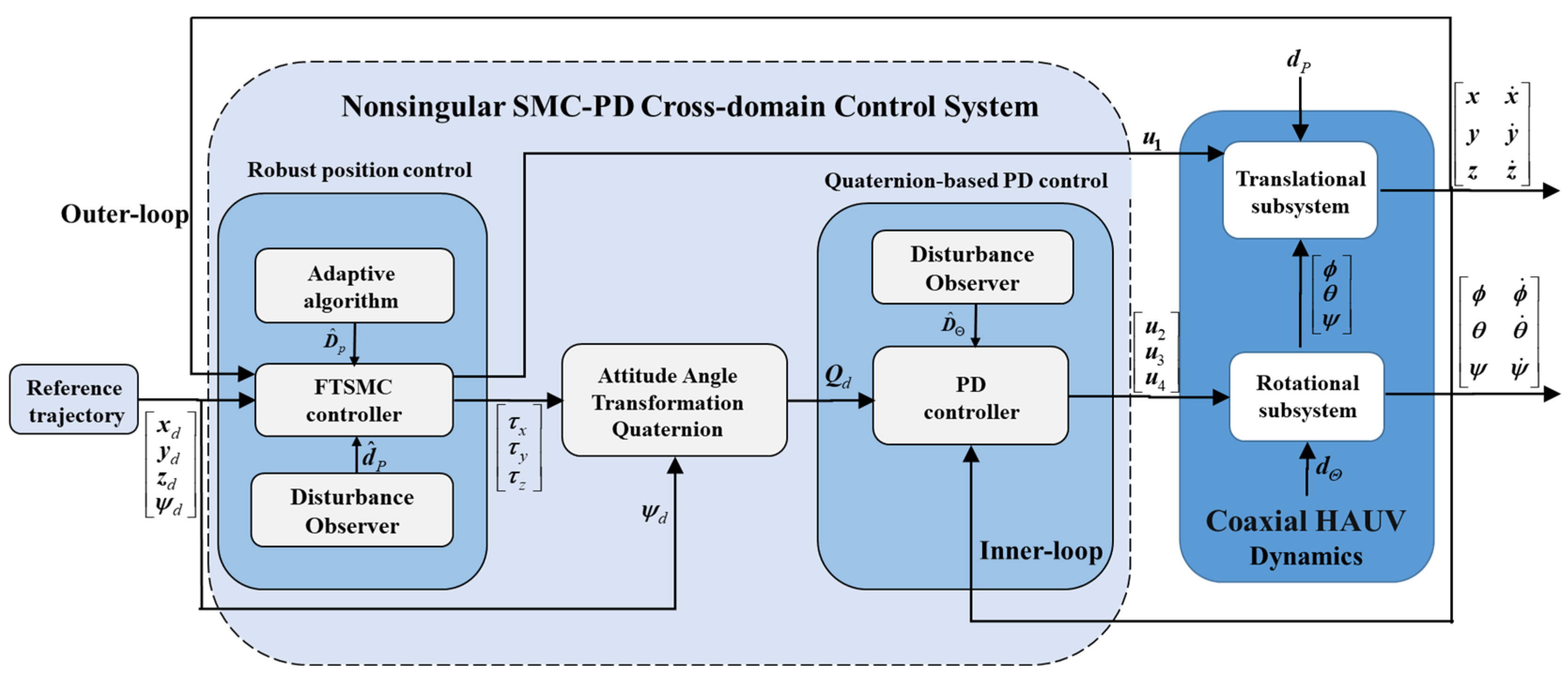
3. Controller Design

The coaxial HAUV is an underactuated 6-DOF motion system with four control inputs: ${\tau }_{\nu }={\left[\begin{array}{cc}{\tau }_{vp}^{\mathrm{T}}& {\tau }_{v\mathrm{\Theta }}^{\mathrm{T}}\end{array}\right]}^{\mathrm{T}}$, ${\tau }_{vp}={\left[\begin{array}{ccc}0& 0& u_1\end{array}\right]}^{\mathrm{T}}$, ${\tau }_{v\mathrm{\Theta }}={\left[\begin{array}{ccc}{u}_2& u_3& u_4\end{array}\right]}^{\mathrm{T}}$. According to the control logic of the coaxial twin-rotor UAV, the controllers are designed for the two systems, respectively, to form a cascade control system. The control scheme frame is shown in Figure 3. A disturbance observer-enhanced adaptive sliding mode controller (DOASMC) was designed for the outer loop to achieve accurate position tracking. The inner loop, which is a feedforward proportion differentiation (PD) controller enhanced by a disturbance observer, was designed.

After the dynamic equation is converted into the inertial coordinate system, the control input of the position subsystem under the inertial system is ${\tau }_p=M_{\eta 1}^{-1}{J}_1^{-\mathrm{T}}{\tau }_{vp}$, where $M_{\eta 1}=J_1^{-\mathrm{T}}{M}_{11}{J}_1^{-1}$. In order to simplify the design of the control system, ${\tau }_p={\left[\begin{array}{ccc}{\tau }_x& {\tau }_y& {\tau }_z\end{array}\right]}^{\mathrm{T}}$ is defined as a virtual control law. The variation in the attitude angle of the coaxial HAUV causes the total lift to produce a horizontal component in the inertial coordinate system, which allows the coaxial HAUV to produce a horizontal maneuver. ${\tau }_p$ is the reason for the horizontal maneuver of the coaxial HAUV.

If the desired ${\psi }_d$ value is given, the total lift force and the expected attitude angle of the attitude subsystem can be obtained.

$$\left\{\begin{array}{l}{u}_1={\tau }_{vp}\left(3\right),{\tau }_{vp}=J_1^T{M}_{\eta 1}{\tau }_p\\ {\theta }_d=\arctan \left({\displaystyle \frac{{\tau }_x\cos {\psi }_d+{\tau }_y\sin {\psi }_d}{{\tau }_z}}\right)\\ {\varphi }_d=\arctan \left({\displaystyle \frac{\left({\tau }_x\sin {\psi }_d-{\tau }_y\cos {\psi }_d\right)\cos {\theta }_d}{{\tau }_z}}\right)\end{array}\right.$$

(32)

3.1. Position Controller Design

3.1.1. The Basic Sliding Mode Controller Frame Design

Define the desired location as ${\eta }_{1d}={\left[\begin{array}{ccc}{x}_d& y_d& z_d\end{array}\right]}^{\mathrm{T}}$; then, the tracking error of the position can be expressed as $e_p={\eta }_1-{\eta }_{1d}={\left[\begin{array}{ccc}{e}_x& e_y& e_z\end{array}\right]}^{\mathrm{T}}$.

First, the finite-time terminal sliding surface based on the learning rate is designed as follows [49]:

$$s_p={\left[\begin{array}{ccc}{s}_x& s_y& s_z\end{array}\right]}^{\mathrm{T}}={\dot{e}}_p+k_1{e}_p+k_2\tanh \left(e_p\right)$$

(33)

where $k_1$, $k_2$ is the parameter matrix of the sliding mode manifold. $k_1$ is the designed parameter based on the learning rate.

$$k_1=k_{10}+\alpha \left|{\dot{e}}_p\right|$$

(34)

where $k_{10}$ is a positive number and $\alpha$ is the learning rate, and its expression is $\alpha =b^{\left|e_p\right|}-1$, satisfying $b>0$, $b\ne 1$.

Remark 5

 ([50]). A variable coefficient $k_1$ is introduced to adjust the speed at which the tracking error converges to zero. The tracking error $e_p$ in the initial stage is large, and the change rate of the tracking error ${\dot{e}}_p$ caused by the controller is also large. The learning rate changes with the error at an exponential rate, which makes the coefficien $k_1$ rise rapidly so that the tracking error converges at a faster rate. However, when the error reaches the sliding mode surface at high speed and the tracking error repeatedly crosses the sliding mode surface, this leads to the system chattering problem. The learning rate will change with the decrease in the tracking error rate so that the coefficient $k_1$ adaptively becomes a small number. The tracking error approaches the surface of the sliding mode at a low speed and effectively inhibits the chattering of the system.

The derivative of the sliding mode variable is calculated as

$$\begin{array}{cc}{\dot{s}}_p& ={\ddot{e}}_p+\left(k_1+k_2\left(1-{\tanh }^{\mathrm{T}}\left(e_p\right)\tanh \left(e_p\right)\right)\right){\dot{e}}_p\\ & =\left({\tau }_p+f_p+{\overline{d}}_p-{\ddot{\eta }}_{1d}\right)+H\left(e_p,{\dot{e}}_p\right)\end{array}$$

(35)

where $H\left(e_p,{\dot{e}}_p\right)=\left(k_1+k_2\left(1-{\tanh }^{\mathrm{T}}\left(e_p\right)\tanh \left(e_p\right)\right)\right){\dot{e}}_p$.

By setting the derivative of the sliding mode variable to 0, the basic finite-time sliding mode controller can be obtained, expressed as follows:

$${\tau }_p=-f_p+{\ddot{\eta }}_{1d}-H\left(e_p,{\dot{e}}_p\right)-k_3{s}_p-D_p\mathrm{sign}\left(s_p\right)$$

(36)

where $k_3$ is a positive constant, and $D_p$ is a sufficiently large constant.

According to the design principle of the sliding mode controller, the main source of its robustness is the switching term $D_p\mathrm{sign}\left(s_p\right)$ with a sign function. If $D_p$ is too large, it will lead to serious chattering of the control signal. In order to ensure the robustness of the controller, a composite robust controller design combining adaptive technology and disturbance observer technology is adopted here.

Remark 6.

The hyperbolic tangent function $\tanh \left(s_i/{\xi }_i\right),{\xi }_i\in \left(0,1\right)$ is used to substitute sign function $\mathrm{sign}\left(s_i\right)$ to weak chattering. It is worth noting that the smaller the value of ${\xi }_i$ is, the closer the properties of the hyperbolic tangent function are to the sign function.

3.1.2. Disturbance Observer Design

A disturbance observer is designed to compensate for lumped uncertainties.

For a classical second-order nonlinear disturbed system,

$$\left\{\begin{array}{l}{\dot{x}}_1=x_2\\ {\dot{x}}_2=f+u+d\end{array}\right.$$

(37)

where $f$, $u$, and $d$ are, respectively, model-related nonlinear functions, control inputs, and uncertainty disturbances.

By introducing the research results of [37], the following disturbance observer can be designed to obtain the observed estimate of uncertainty.

$$\left\{\begin{array}{l}\dot{\widehat{d}}=-{\kappa }_1\left(\widehat{v}-x_2\right)\\ \dot{\widehat{v}}=f+u+\widehat{d}-{\kappa }_2\left(\widehat{v}-x_2\right)\end{array}\right.$$

(38)

where $\widehat{d}$ is the estimate of $d$ and $\widehat{v}$ is the estimate of $x_2$; ${\kappa }_1>0$ and ${\kappa }_2>0$ represent observer gain.

The Lyapunov function for stability analysis is selected as follows:

$$V={\displaystyle \frac{1}{2{\kappa }_1}}{\tilde{d}}_p^2+{\displaystyle \frac{1}{2}}{\tilde{v}}^2$$

(39)

where $\tilde{d}=d-\widehat{d},\tilde{v}=v-\widehat{v}$.

By taking the derivative of the designed Lyapunov function and considering Assumption 2,

$$\begin{array}{cc}\dot{V}& ={\displaystyle \frac{1}{{\kappa }_1}}{\tilde{d}}_p{\dot{\tilde{d}}}_p+\tilde{v}\dot{\tilde{v}}={\displaystyle \frac{1}{{\kappa }_1}}{\tilde{d}}_p\left({\dot{d}}_p-{\dot{\widehat{d}}}_p\right)+\tilde{v}\left(\ddot{p}-\dot{\widehat{v}}\right)\\ & =-{\displaystyle \frac{1}{{\kappa }_1}}{\tilde{d}}_p{\dot{\widehat{d}}}_p+\tilde{v}\left(\ddot{p}-\dot{\widehat{v}}\right)\end{array}$$

(40)

Substituting Equation (38) into Equation (41) yields

$$\begin{array}{cc}\dot{V}& =-{\displaystyle \frac{1}{{\kappa }_1}}{\tilde{d}}_p\left(-{\kappa }_1\left(\widehat{v}-\dot{p}\right)\right)+\tilde{v}\left(\left(v_p+f_p+d_p\right)-\left(v_p+f_p+{\widehat{d}}_p-{\kappa }_2\left(\widehat{v}-\dot{p}\right)\right)\right)\\ & ={\tilde{d}}_p\left(\widehat{v}-\dot{p}\right)+\tilde{v}\left(d_p-{\widehat{d}}_p+{\kappa }_2\left(\widehat{v}-\dot{p}\right)\right)\\ & =-{\tilde{d}}_p\tilde{v}+{\tilde{d}}_p\tilde{v}-{\kappa }_2{\tilde{v}}^2\\ & =-{\kappa }_2{\tilde{v}}^2\le 0\end{array}$$

(41)

When $\dot{V}\equiv 0$, the following relationship holds: $\tilde{v}\equiv 0$, $\dot{\tilde{v}}\equiv 0$, ${\tilde{d}}_p\equiv 0$. According to LaSalle’s invariance theorem, $t\to \infty$, ${\tilde{d}}_p\to 0$. The above derivation proves that the $d_p$ term can be effectively observed by the disturbance observer.

Through the above analysis, the disturbance observer designed for the position subsystem of Equation (25) is as follows:

$$\left\{\begin{array}{l}{\dot{\widehat{\overline{d}}}}_p=-{\kappa }_1\left({\widehat{v}}_{1I}-v_{1I}\right)\\ {\dot{\widehat{v}}}_{1I}={\tau }_p+f_p+{\widehat{\overline{d}}}_p-{\kappa }_2\left({\widehat{v}}_{1I}-v_{1I}\right)\end{array}\right.$$

(42)

where ${\widehat{\overline{d}}}_p$ is the estimate of the ${\overline{d}}_p$ items, and ${\widehat{v}}_{1I}$ is the estimate of $v_{1I}$. It is worth noting that the observation ${\widehat{\overline{d}}}_p$ obtained by the observer above is the observation value of uncertainty ${\overline{d}}_p$ under the inertial frame. According to the relation ${\overline{d}}_p=M_{\eta 11}^{-1}{J}_1^{-\mathrm{T}}{d}_p$ in Equation (25), ${\widehat{d}}_p=J_1^{\mathrm{T}}{M}_{\eta 11}{\widehat{\overline{d}}}_p$ should be obtained via mathematical transformation.

Similarly, the disturbance observer designed for the attitude subsystem of Equation (29) is as follows:

$$\left\{\begin{array}{l}{\dot{\widehat{d}}}_{\mathrm{\Theta }}=-{\kappa }_1{I}_w\left(\widehat{\omega }-\omega \right)\\ \dot{\widehat{\omega }}=I_w^{-1}\left(f_{\mathrm{\Theta }}+{\tau }_{\mathrm{\Theta }}+{\widehat{d}}_{\mathrm{\Theta }}\right)-{\kappa }_2\left(\widehat{\omega }-\omega \right)\end{array}\right.$$

(43)

where ${\widehat{d}}_{\mathrm{\Theta }}$ is the estimate of the $d_{\mathrm{\Theta }}$ items, and $\widehat{\omega }$ is the estimate of $\omega$.

3.1.3. Adaptive Law Design

By introducing DO into the controller to compensate the system uncertainty, the robustness of the controller is improved. In addition, the introduction of DO greatly alleviates the requirement of switching gain in traditional sliding mode control. Further, an adaptive law is designed to compensate the observation error of the DO. The combination of the observer and the adaptive technique can effectively reduce the chattering of the system.

$$\left\{\begin{array}{l}{\dot{\widehat{D}}}_p={\left[\begin{array}{ccc}{\dot{\widehat{D}}}_x& {\dot{\widehat{D}}}_y& {\dot{\widehat{D}}}_z\end{array}\right]}^{\mathrm{T}}\\ {\dot{\widehat{D}}}_i={\gamma }_1\left(\left|s_i\right|-{\gamma }_2{\widehat{D}}_i\right),i=x,y,z\end{array}\right.$$

(44)

where ${\widehat{D}}_p$ is the estimation value of $D_p$. The function of ${\widehat{D}}_p$ is designed to compensate for the observation error, and ${\gamma }_1>0$, ${\gamma }_2>0$ represents the adaptive law adjusting parameters.

3.1.4. Synthesis of Composite Robust Controller

Finally, the position composite robust controller can be designed as

$${\tau }_p=-f_p-{\widehat{\overline{d}}}_p+{\ddot{\eta }}_{1d}-H\left(e_p,{\dot{e}}_p\right)-k_3{s}_p-\left({\widehat{D}}_p+{\delta }_p\right)\mathrm{sign}\left(s_p\right)$$

(45)

where ${\delta }_p\in R^3$ is a positive number.

Considering that the control inputs ${\tau }_p$ are under the inertial system, then the actual control input can be calculated as follows:

$$\left\{\begin{array}{l}{\tau }_{vp}=J_1^{\mathrm{T}}{M}_{\eta 1}{\tau }_p\\ M_{\eta 1}=J_1^{-\mathrm{T}}{M}_{11}{J}_1^{-1}\end{array}\right.$$

(46)

3.2. Attitude Controller Design Based on Quaternion

3.2.1. Transformation of the Euler Angle to the Quaternion Control Target

The relationship between ${\eta }_2$ and $Q$ can be derived from Equations (30) and (31), and the relationship between $\varpi$ and ${\dot{q}}_v$ can be derived from Equation (29). Therefore, the control problem for the Euler angle and angular velocity can be transformed into the control problem for $\tilde{Q}$ and $\tilde{\varpi }$.

The desired attitude angle is expressed as ${\eta }_{2d}={\left[\begin{array}{ccc}{\varphi }_d& {\theta }_d& {\psi }_d\end{array}\right]}^T$; then, we can obtain $Q_d={\left[\begin{array}{cc}{q}_{0d}& q_{vd}^{\mathrm{T}}\end{array}\right]}^{\mathrm{T}}$ and $\tilde{Q}={\left[\begin{array}{cc}{\tilde{q}}_0& {\tilde{q}}_v^{\mathrm{T}}\end{array}\right]}^{\mathrm{T}}$, ${\tilde{q}}_v={\left[\begin{array}{ccc}{\tilde{q}}_1& {\tilde{q}}_2& {\tilde{q}}_3\end{array}\right]}^{\mathrm{T}}$.

According to the rules of quaternions, we satisfy the following relationships:

$$\left\{\begin{array}{l}{\tilde{q}}_0=q_0{q}_{0d}+q_{vd}^{\mathrm{T}}{q}_v\\ {\tilde{q}}_v=q_{0d}{q}_v-q_0{q}_{vd}-q_v^{\times }{q}_{vd}\\ {\tilde{q}}_0^2+{\tilde{q}}_v^{\mathrm{T}}{\tilde{q}}_v=1,\\ {\dot{\tilde{q}}}_0=-{\displaystyle \frac{1}{2}}{\tilde{q}}_v^{\mathrm{T}}\tilde{\omega },{\dot{\tilde{q}}}_v=G\tilde{\omega },\\ G={\displaystyle \frac{1}{2}}({\tilde{q}}_0{I}_3+{\tilde{q}}_v^{\times }),\tilde{\omega }=\omega -R(\tilde{Q}){\omega }_d\\ R(\tilde{Q})=\left({\tilde{q}}_0^2-{\tilde{q}}_v^{\mathrm{T}}{\tilde{q}}_v\right)I_3+2{\tilde{q}}_v{\tilde{q}}_v^{\mathrm{T}}-2{\tilde{q}}_0{\tilde{q}}_v^{\times }\end{array}\right.$$

(47)

Let us define a new quaternion error equation: $Q_e={\left[\begin{array}{cc}1-{\tilde{q}}_0& {\tilde{q}}_v^{\mathrm{T}}\end{array}\right]}^{\mathrm{T}}$; the control objective can be modified as follows:

$$\underset{t\to \infty }{\lim }{Q}_e=0,\underset{t\to \infty }{\lim }\tilde{\omega }=0$$

(48)

That is, ${\tilde{q}}_v\to 0$, ${\tilde{q}}_0\to 1$, $\tilde{\omega }\to 0$.

3.2.2. Design of Fast and Robust Feedforward PD Controller Based on the Learning Rate

According to the analysis in the previous section, the effect of controlling the quaternion and Euler angle in the attitude system can be converted equally. Generally speaking, the response speed of the inner loop of the cascade control system is faster than that of the outer loop, so the PD control frame with a simple structure and fast response is used to design the attitude quaternion controller. The PD control algorithm is a very classical linear control algorithm; the function of the proportion (P) term is to promote the control error to converge quickly to zero; the function of the differentiation (D) term is similar to the “brake”, for which the hysteresis error overshoot fluctuation is around 0. A basic feedforward PD control law is designed as follows [16,33]:

$${\tau }_{v\mathrm{\Theta }}=-k_p{\tilde{q}}_v-k_d\tilde{\omega }-f_{\mathrm{\Theta }}$$

(49)

In order to further improve the convergence speed of control errors, the design idea of the learning rate is introduced into the design of the P-term parameters. At the same time, a disturbance observer is introduced to estimate the uncertainty of the attitude subsystem, which further improves the robustness of the feedforward PD algorithm.

$${\tau }_{v\mathrm{\Theta }}=-k_p{\tilde{q}}_v-k_d\tilde{\omega }-f_{\mathrm{\Theta }}-{\widehat{d}}_{\mathrm{\Theta }}$$

(50)

Based on the idea of the learning rate, the design of the P term is as follows:

$$k_p=k_{p0}+\alpha \left|\tilde{\omega }\right|$$

(51)

where $k_{p0}>0$ is the value of the basic P item, $\alpha$ is the learning rate, and its expression is $\alpha =b^{\left|{\tilde{q}}_v\right|}-1$, which satisfies $b>0$, $b\ne 1$.

3.3. Controller Stability Analysis

Theorem 1.

Consider the position of subsystem (25) A, where an observer enhanced adaptive composite finite-time terminal sliding mode controller (45) is employed. Then, the sliding mode surface will reach the neighborhood of 0 in finite time, $T_1$. Once the sliding mode surface $s_p=0$ is satisfied, the error $e_p$ also converges to 0 in a finite time, $T_2$.

Proof of Theorem 1.

The proof process has the following two steps: the first step proves that the arrival stage sliding surface can be reached, $s_p=0$, in a finite time, $T_1$. The second step proves that the tracking error $e_p$ in the sliding stage can converge to the neighborhood of 0 in finite time, $T_2$. □

The Lyapunov function is designed as follows:

$$V_p={\displaystyle \frac{1}{2}}{s}_p^{\mathrm{T}}{s}_p+{\displaystyle \frac{1}{2{\gamma }_1}}{\tilde{D}}_p^{\mathrm{T}}{\tilde{D}}_p$$

(52)

By taking the derivative of the Lyapunov function, we obtain

$$\begin{array}{cc}{\dot{V}}_p& =s_p^{\mathrm{T}}{\dot{s}}_p-{\displaystyle \frac{1}{{\gamma }_1}}{\tilde{D}}_p^{\mathrm{T}}{\dot{\widehat{D}}}_p\\ & =s_p^{\mathrm{T}}{\dot{s}}_p-{\displaystyle \frac{1}{{\gamma }_1}}{\displaystyle \sum _{i=1}^3{\tilde{D}}_i{\dot{\widehat{D}}}_i}\end{array}$$

(53)

By substituting the derivative of the sliding mode variable (38) and the controller (45) into the above equation, one obtains

$$\begin{array}{cc}{\dot{V}}_p& =s_p^{\mathrm{T}}\left({\ddot{e}}_p+H\left(e_p,{\dot{e}}_p\right)\right)-{\displaystyle \frac{1}{{\gamma }_1}}{\displaystyle \sum _{i=1}^3{\tilde{D}}_i{\dot{\widehat{D}}}_i}\\ & =s_p^{\mathrm{T}}\left(\left({\tau }_p+f_p+{\overline{d}}_p-{\ddot{\eta }}_{1d}\right)+H\left(e_p,{\dot{e}}_p\right)\right)-{\displaystyle \frac{1}{{\gamma }_1}}{\displaystyle \sum _{i=1}^3{\tilde{D}}_i{\dot{\widehat{D}}}_i}\\ & =s_p^{\mathrm{T}}\left({\overline{d}}_p-{\widehat{\overline{d}}}_p-k_3{s}_p-\left({\widehat{D}}_p+{\delta }_p\right)\mathrm{sign}\left(s_p\right)\right)-{\displaystyle \frac{1}{{\gamma }_1}}{\displaystyle \sum _{i=1}^3{\tilde{D}}_i{\dot{\widehat{D}}}_i}\\ & =s_p^{\mathrm{T}}\left({\tilde{\overline{d}}}_p-k_3{s}_p-\left({\widehat{D}}_p+{\delta }_p\right)\mathrm{sign}\left(s_p\right)\right)-{\displaystyle \frac{1}{{\gamma }_1}}{\displaystyle \sum _{i=1}^3{\tilde{D}}_i{\dot{\widehat{D}}}_i}\\ & \le -k_3{‖s_p‖}^2-{\delta }_p‖s_p‖+{\displaystyle \sum _{i=1}^3\left|s_i\right|\left(\left|{\tilde{\overline{d}}}_i\right|-{\widehat{D}}_i\right)}-{\displaystyle \frac{1}{{\gamma }_1}}{\displaystyle \sum _{i=1}^3{\tilde{D}}_i{\dot{\widehat{D}}}_i}\\ & \le -k_3{‖s_p‖}^2-{\delta }_p‖s_p‖+{\displaystyle \sum _{i=1}^3\left|s_i\right|{\tilde{D}}_i}-{\displaystyle \frac{1}{{\gamma }_1}}{\displaystyle \sum _{i=1}^3{\tilde{D}}_i{\dot{\widehat{D}}}_i}\end{array}$$

(54)

In the previous discussion, we discussed that a coaxial HAUV suffers from more complex perturbations and parameter perturbations than traditional UUVs and UAVs. The use of observer observation to compensate for external perturbations is not enough to completely offset the effect of complex perturbations. Therefore, adaptive technology is adopted to further compensate for the remaining residual terms ${\tilde{\overline{d}}}_p$, and $\left(\left|{\tilde{\overline{d}}}_i\right|-{\widehat{D}}_i\right)$ is redefined as ${\tilde{D}}_i$.

By substituting the adaptive law (44) into Equation (54),

$$\begin{array}{cc}{\dot{V}}_p& \le -k_3{‖s_p‖}^2-{\delta }_p‖s_p‖+{\displaystyle \sum _{i=1}^3\left|s_i\right|{\tilde{D}}_i}-{\displaystyle \frac{{\gamma }_1}{{\gamma }_1}}{\displaystyle \sum _{i=1}^3{\tilde{D}}_i\left(\left|s_i\right|-{\gamma }_2{\widehat{D}}_i\right)}\\ & \le -k_3{‖s_p‖}^2-{\delta }_p‖s_p‖+{\gamma }_2{\displaystyle \sum _{i=1}^3{\tilde{D}}_i{\widehat{D}}_i}\end{array}$$

(55)

According to Young’s inequality, the term ${\tilde{D}}_i{\widehat{D}}_i$ satisfies the following relation:

$$\begin{array}{cc}{\tilde{D}}_i{\widehat{D}}_i& ={\tilde{D}}_i\left(D_i-{\tilde{D}}_i\right)\\ & =-{\tilde{D}}_i^2+{\tilde{D}}_i{D}_i\\ & \le -{\tilde{D}}_i^2+\left({\tilde{D}}_i^2/2+D_i^2/2\right)\\ & \le -{\tilde{D}}_i^2/2+D_i^2/2\end{array}$$

(56)

A further simplified representation can be obtained:

$$\begin{array}{cc}{\dot{V}}_p& \le -k_3{‖s_p‖}^2-{\displaystyle \frac{{\gamma }_2}{2}}{\displaystyle \sum _{i=1}^3\left({\tilde{D}}_i^2-D_i^2\right)}\\ & \le -k_3{s}_p^{\mathrm{T}}{s}_p-{\displaystyle \frac{{\gamma }_2}{2}}{\tilde{D}}_p^{\mathrm{T}}{\tilde{D}}_p+{\displaystyle \frac{{\gamma }_2}{2}}{\displaystyle \sum _{i=1}^3{D}_i^2}\\ & \le -{\lambda }_p{V}_p+{\Delta }_p\end{array}$$

(57)

where ${\lambda }_p=\min \left\{2k_3,{\gamma }_1{\gamma }_2\right\}$, ${\Delta }_p={\displaystyle \frac{{\gamma }_2}{2}}{\displaystyle \sum _{i=1}^3{D}_i^2}$.

According to the Lyapunov stability criterion and Lemma 2, the above proof process only verifies the asymptotic stability of the system in a strict sense; then, $s_p$ and ${\tilde{D}}_p$ are uniformly and terminally bounded.

The actual finite time stability of the closed-loop system will be proved next. In order to prove the finite time convergence of error variables more precisely, the new Lyapunov function is chosen as

$$V_{p1}={\displaystyle \frac{1}{2}}{s}_p^{\mathrm{T}}{s}_p$$

(58)

Taking the derivative of the Lyapunov function, we obtain

$$\begin{array}{cc}{\dot{V}}_{p1}& =s_p^{\mathrm{T}}\left({\ddot{e}}_p+H\left(e_p,{\dot{e}}_p\right)\right)\\ & =s_p^{\mathrm{T}}\left(\left({\tau }_p+f_p+{\overline{d}}_p-{\ddot{\eta }}_{1d}\right)+H\left(e_p,{\dot{e}}_p\right)\right)\end{array}$$

(59)

By substituting the derivative of the sliding mode variable and the controller into the above equation, we can obtain

$$\begin{array}{cc}{\dot{V}}_{p1}& =s_p^{\mathrm{T}}\left({\overline{d}}_p-{\widehat{\overline{d}}}_p-k_3{s}_p-\left({\widehat{D}}_p+{\delta }_p\right)\mathrm{sign}\left(s_p\right)\right)\\ & =s_p^{\mathrm{T}}\left({\tilde{\overline{d}}}_p-k_3{s}_p-\left({\widehat{D}}_p+{\delta }_p\right)\mathrm{sign}\left(s_p\right)\right)\\ & \le -k_3{‖s_p‖}^2-{\delta }_p‖s_p‖+{\displaystyle \sum _{i=1}^3\left|s_i\right|\left(\left|{\tilde{\overline{d}}}_i\right|-{\widehat{D}}_i\right)}\\ & \le -k_3{‖s_p‖}^2-{\delta }_p‖s_p‖+{\displaystyle \sum _{i=1}^3\left|s_i\right|{\tilde{D}}_i}\end{array}$$

(60)

Since it has been proved that the estimation error ${\tilde{D}}_p$ and the sliding mode surface $s_p$ are bounded, then ${\displaystyle \sum _{i=1}^3\left(\left|s_i\right|{\tilde{D}}_i\right)}$ is also bounded. The above inequality can be further rewritten as

$$\begin{array}{c}{\dot{V}}_{p1}\le -{\delta }_p‖s_p‖+{\displaystyle \sum _{i=1}^3\left|s_i\right|{\tilde{D}}_i}\\ \le -{\lambda }_{p1}{\dot{V}}_{p1}^{{\displaystyle \frac{1}{2}}}+{\Delta }_{p1}\end{array}$$

(61)

where ${\lambda }_{p1}=\sqrt{2}{\delta }_p$, ${\Delta }_{p1}={\displaystyle \sum _{i=1}^3\left|s_i\right|{\tilde{D}}_i}$. According to (61), by using the Lyapunov stability criterion and Lemma 1, it can be concluded that the sliding mode manifold converges to zero in finite time. Once the end of the phase is reached, the error variable will converge to zero in a finite time along the sliding mode surface. The above proves the error convergence characteristic of the position subsystem in finite time.

Theorem 2.

Consider the attitude subsystem (32), where the quaternion-based feedforward PD controller (50) is used. Then, the quaternion error $\tilde{Q}={\left[\begin{array}{cc}{\tilde{q}}_0& {\tilde{q}}_v^{\mathrm{T}}\end{array}\right]}^{\mathrm{T}}$ and angular velocity error $\tilde{\omega }$ converge to 0 progressively, which also ensures that the transformed Euler angle tracking error ${\eta }_{2e}$ converge to 0 asymptotically.

Proof of Theorem 2.

The Lyapunov function is designed as

$$V_{\mathrm{\Theta }}=V_{\mathrm{\Theta }1}+V_{\mathrm{\Theta }2}$$

(62)

where $V_{\mathrm{\Theta }1}={\tilde{\omega }}^{\mathrm{T}}{I}_w\tilde{\omega }$, $V_{\mathrm{\Theta }2}=k_p{Q}_e^{\mathrm{T}}{Q}_e$.□

According to the cross-product rule, $a\cdot \left(a\times c\right)=c\cdot \left(a\times a\right)=0$, and as a result, ${\tilde{\omega }}^{\mathrm{T}}\tilde{\omega }\times \left(I_w\tilde{\omega }\right)=0$, ${\tilde{q}}_v^{\mathrm{T}}{\tilde{q}}_v^{\times }={\left[\begin{array}{ccc}0& 0& 0\end{array}\right]}^{\mathrm{T}}$. Let ${\omega }_d=0$; then, $\tilde{\omega }=\omega -R(\tilde{Q}){\omega }_d=\omega$, and $\dot{\tilde{\omega }}=\dot{\omega }$.

By taking the derivative of $V_{\mathrm{\Theta }1}$ and $V_{\mathrm{\Theta }2}$ separately, we obtain

$$\begin{array}{cc}{\dot{V}}_{\mathrm{\Theta }1}& ={\tilde{\omega }}^{\mathrm{T}}{I}_w\dot{\tilde{\omega }}\\ & ={\tilde{\omega }}^{\mathrm{T}}\left(f_{\mathrm{\Theta }}+{\tau }_{v\mathrm{\Theta }}+d_{\mathrm{\Theta }}\right)\end{array}$$

(63)

$$\begin{array}{cc}{\dot{V}}_{\mathrm{\Theta }2}& =2k_p{Q}_e^{\mathrm{T}}{\dot{Q}}_e=2k_p\left[\begin{array}{cc}1-{\tilde{q}}_0& {\tilde{q}}_v^{\mathrm{T}}\end{array}\right]{\left[\begin{array}{cc}-{\dot{\tilde{q}}}_0& {\dot{\tilde{q}}}_v^{\mathrm{T}}\end{array}\right]}^{\mathrm{T}}\\ & =2k_p\left[\begin{array}{cc}1-{\tilde{q}}_0& {\tilde{q}}_v^{\mathrm{T}}\end{array}\right]{\left[\begin{array}{cc}{\displaystyle \frac{1}{2}}{\tilde{q}}_v^{\mathrm{T}}\tilde{\omega }& {\left(G\tilde{\omega }\right)}^{\mathrm{T}}\end{array}\right]}^{\mathrm{T}}\\ & =k_p\left(1-{\tilde{q}}_0\right){\tilde{q}}_v^{\mathrm{T}}\tilde{\omega }+{\kappa }_p{\tilde{q}}_v^{\mathrm{T}}({\tilde{q}}_0{I}_3+{\tilde{q}}_v^{\times })\tilde{\omega }\\ & =k_p{\tilde{q}}_v^{\mathrm{T}}\tilde{\omega }\end{array}$$

(64)

According to the above calculation, the derivative of the Lyapunov function can be obtained. Then, the controller (50) is substituted into (63) to obtain the following equation:

$$\begin{array}{cc}{\dot{V}}_{\mathrm{\Theta }}& ={\dot{V}}_{\mathrm{\Theta }1}+{\dot{V}}_{\mathrm{\Theta }2}\\ & ={\tilde{\omega }}^{\mathrm{T}}\left(f_{\mathrm{\Theta }}+{\tau }_{v\mathrm{\Theta }}+d_{\mathrm{\Theta }}\right)+k_p{\tilde{q}}_v^{\mathrm{T}}\tilde{\omega }\\ & ={\tilde{\omega }}^{\mathrm{T}}\left(f_{\mathrm{\Theta }}+d_{\mathrm{\Theta }}-k_p{\tilde{q}}_v-k_d\tilde{\omega }-f_{\mathrm{\Theta }}-{\widehat{d}}_{\mathrm{\Theta }}\right)+k_p{\tilde{q}}_v^{\mathrm{T}}\tilde{\omega }\\ & ={\tilde{\omega }}^{\mathrm{T}}\left(-k_d\tilde{\omega }\right)\\ & =-k_d{\tilde{\omega }}^{\mathrm{T}}\tilde{\omega }\le 0\end{array}$$

(65)

Because of ${\omega }_d=0$, $\tilde{\omega }=\omega -R(\tilde{Q}){\omega }_d=\omega$, $\dot{\tilde{\omega }}=\dot{\omega }$. According to Lassale’s theorem, if we verify ${\dot{V}}_{\mathrm{\Theta }}\equiv 0$, then $\tilde{\omega }\equiv 0$; thus, $\omega \equiv 0,\dot{\omega }\equiv 0$. We can further obtain ${\tilde{q}}_v=0$. When $t\to \infty$, ${\tilde{q}}_v=0$, ${\tilde{q}}_0=1$, $\tilde{\omega }=0$; this also ensures that the Euler angle tracking error ${\eta }_{2e}$ gradually converges to 0 [35,51,52].

4. Simulation and Discussion

Based on the above theoretical analysis, we theoretically analyze the effectiveness of the observer enhanced cascade SMC-PD algorithm. In this section, some simulation results are given to prove the performance of the proposed control method. Next, we conducted simulations of HAUV motion control and selected the two most typical working conditions (3D spiral water exit and vertical climb water exit) to verify the robustness of the proposed control strategy in dealing with coaxial HAUV cross-media motion with environmental disturbance and parameter perturbation. The controller parameters used in our simulation are given in

Table 1. Control system parameters.

	Parameter Symbol	Value	Parameter Symbol	Value
controller parameter	$k_{10}$	1.5	$k_3$	5
	$k_2$	1.5	${\delta }_p$	0.1
	$k_{p0}$	210	$k_d$	6
disturbance observer	${\kappa }_1$	$5000\cdot I^{3\times 3}$	${\kappa }_2$	$50\cdot I^{3\times 3}$
adaptive law	${\gamma }_1$	1.5	${\gamma }_2$	0.002
learning rate	$b$	45	$\xi$	0.1

.

$k_{10}$$k_3$$k_2$${\delta }_p$$k_{p0}$$k_d$${\kappa }_1$$5000\cdot I^{3\times 3}$${\kappa }_2$$50\cdot I^{3\times 3}$${\gamma }_1$${\gamma }_2$$b$$\xi$ The wind, wave, and current interference parameters used in the simulation are given in Appendix A. At the same time, the lumped uncertainty is described in advance as the form of a random function:

$$\left\{\begin{array}{l}{d}_x=1.3sin\left(0.1\pi t\right)+0.3cos\left(0.13\pi t\right)+0.1k_s\\ d_y=1.3cos\left(0.12\pi t\right)+0.3sin\left(0.12\pi t\right)+0.1k_s\\ d_z=1.3sin\left(0.13\pi t\right)+0.3cos\left(0.1\pi t\right)+0.1k_s\\ d_{\varphi }=0.5sin\left(0.21\pi t\right)+0.1cos\left(0.41\pi t\right)\\ d_{\theta }=0.5sin\left(0.31\pi t\right)+0.1cos\left(0.31\pi t\right)\\ d_{\psi }=0.5cos\left(0.41\pi t\right)+0.1cos\left(0.21\pi t\right)\end{array}\right.$$

(66)

The initial status is set as ${\left[x_0,y_0,z_0,{\dot{x}}_0,{\dot{y}}_0,{\dot{z}}_0\right]}^{\mathrm{T}}={\left[0.2,1.8,-21,0,0,0\right]}^{\mathrm{T}}$, considering the constraint rule condition of quaternion $q_0^2+q_v^{\mathrm{T}}{q}_v=1$; take the initial state of the quaternion as $Q_0={\left[0.8,0.4,0.4,0.2\right]}^{\mathrm{T}}$. Because of the transformation relationship, the initial value of the defined quaternion $Q_0$ is equivalent to the initial value of the defined Euler angle. The initial value of the angular velocity is set as ${\omega }_0={\left[0.1,0.1,0.1\right]}^{\mathrm{T}}$.

In order to conduct a comparative study, the basic controller in [16] was selected as the control group to verify the superiority of the designed DO-enhanced SMC-PD controller. The basic controller adopts the PID-PD control algorithm, that is, the position loop and the attitude loop adopt the gain-adjustment PID algorithm and PD algorithm, respectively. The following two classical cases (spiral cross-domain maneuver and vertical cross-domain maneuver) were simulated comprehensively to explain the superiority of our proposed controller and compare which cross-domain maneuver trajectory is better.

4.1. Working Case 1 (Spiral Climbing Trajectory)

The trajectory of selected working case 1 is shown in the following equation:

$$\left\{\begin{array}{l}{x}_d=2\sin \left(0.1\pi t\right)\\ y_d=2\cos \left(0.1\pi t\right)\\ z_d=0.1t-2\\ {\phi }_d=0.01\end{array}\right.$$

(67)

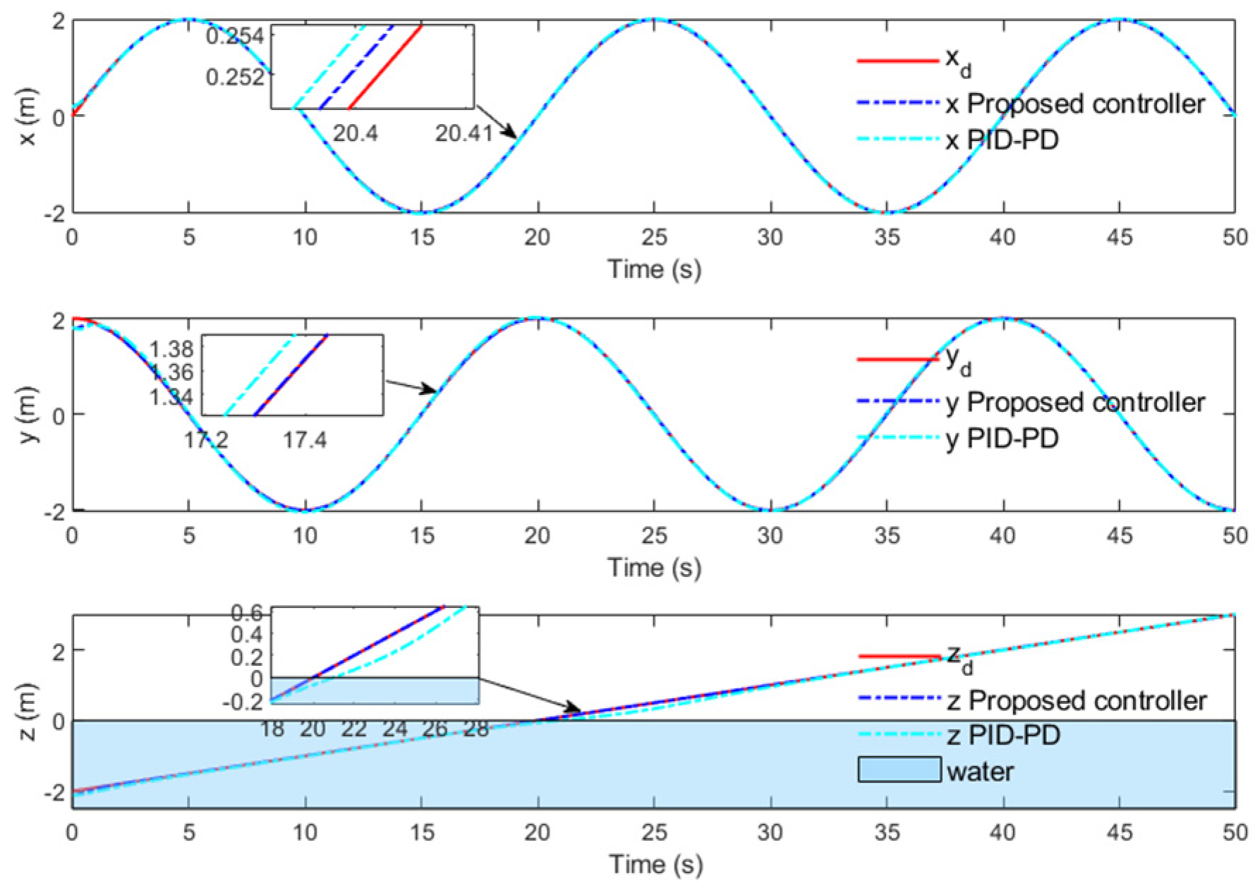
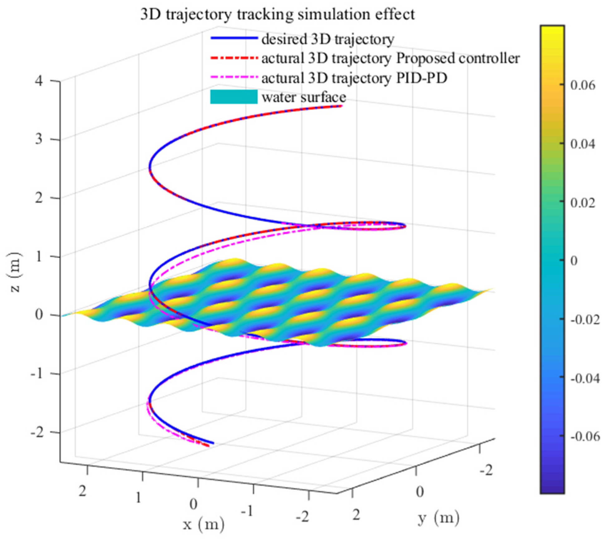
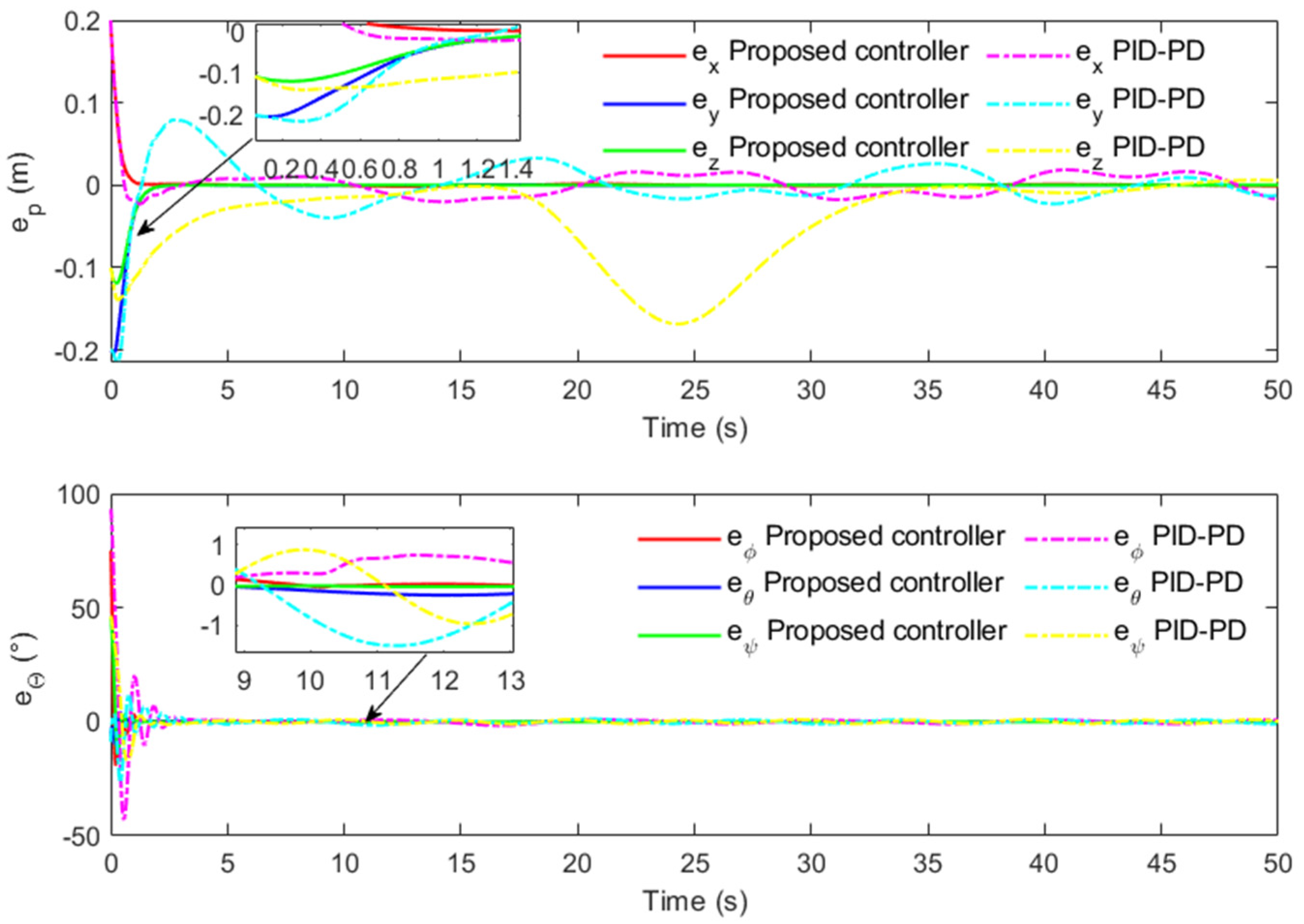
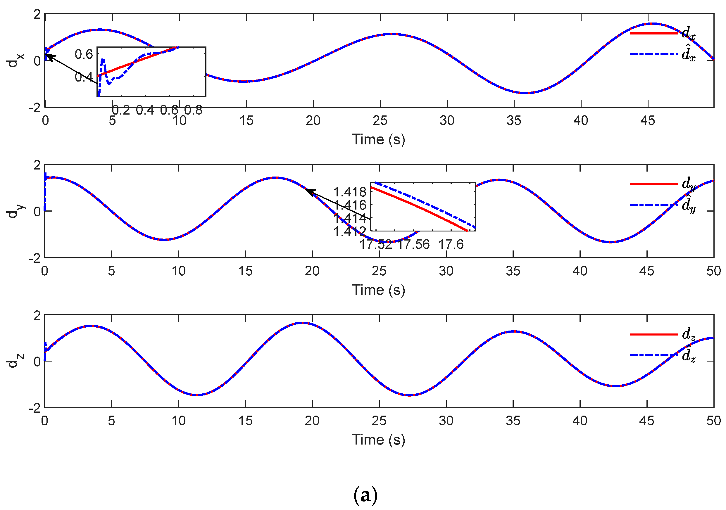
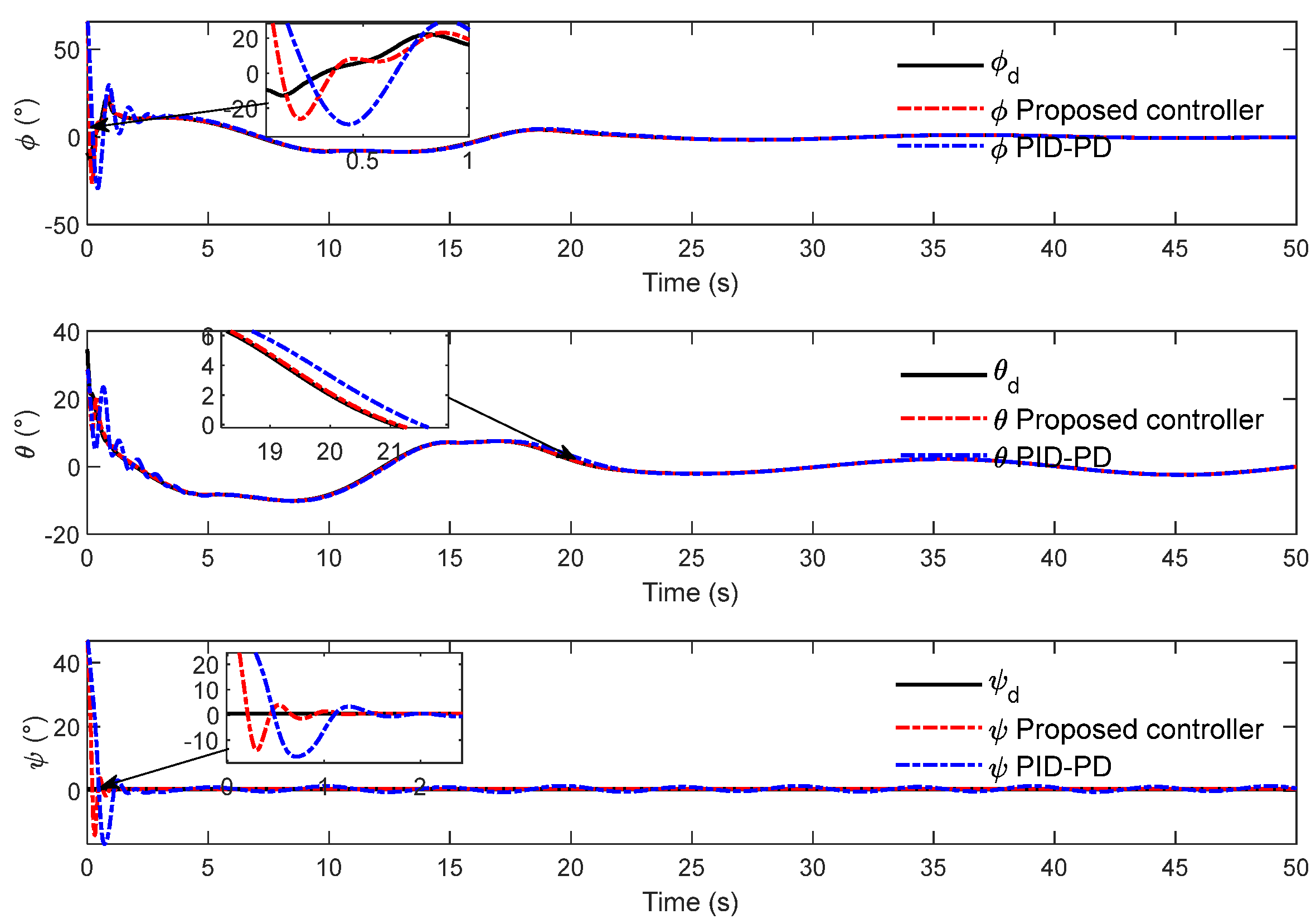
The main purpose of the trajectory design is to test the ability of the controller to track the trajectory in 3D space. Figure 4 and Figure 5 show the tracking response of the position loop with the proposed controller and basic controller. It can be clearly seen that the proposed composite robust controller performs well under time-varying system model parameters and external disturbances. Figure 4 shows the tracking evolution results of the three channels of translation motion over time. Although a good tracking effect can be obtained for each channel under the action of two controllers, it can be seen from local magnification that the HAUV can track the desired trajectory more accurately under the proposed controller. It can be seen in Figure 5 that the HAUV trajectory starts from underwater through the wave surface and spirals up into the air, showing a good 3D tracking effect in the whole process. 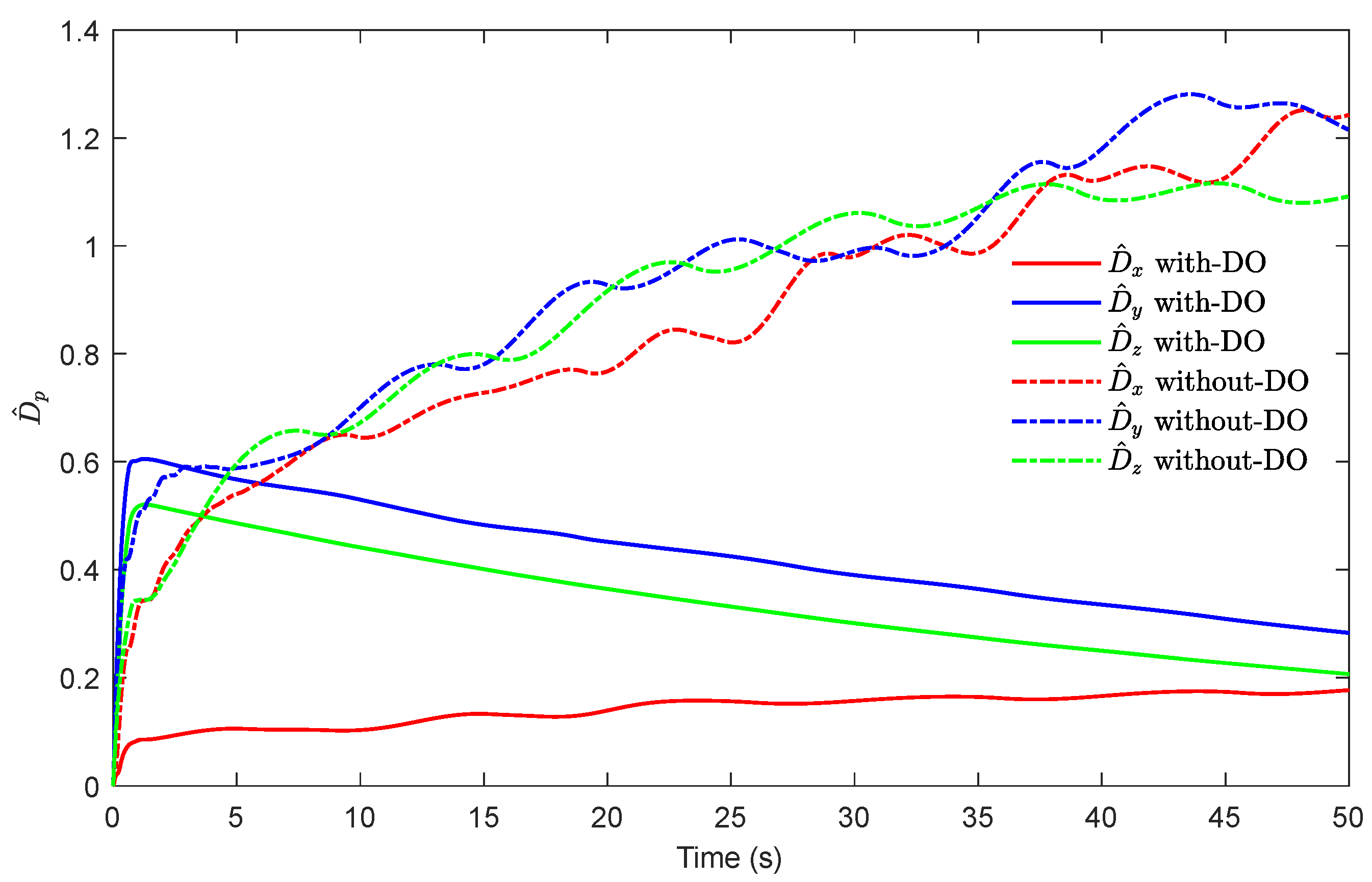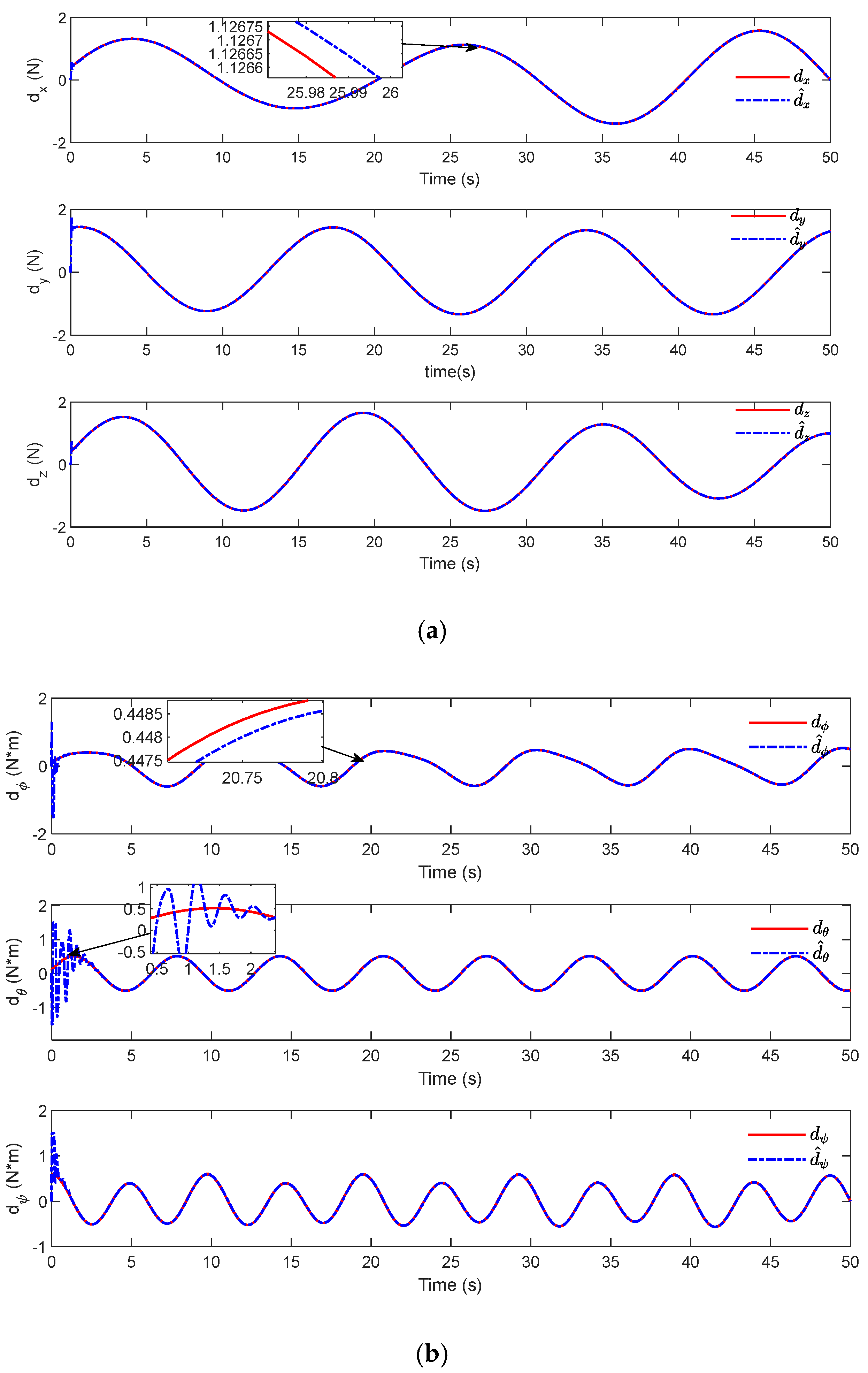Figure 6 shows the effect diagram of the proposed observer’s observation results for the unknown disturbance and the set value comparison. It can be seen in the estimation results that although the initial value of the observer is quite different from the observed disturbance value, and the accurate observation value is quickly obtained. The estimation error can be quickly reduced, which proves that the proposed observer can provide reliable disturbance estimation values for the controller design. In the local magnification image, the observer produces large fluctuations in the initial stage, and the actual observation error is not strictly 0 in the steady state stage. Here, the adaptive parameter evolution results after removing DO are also tested. 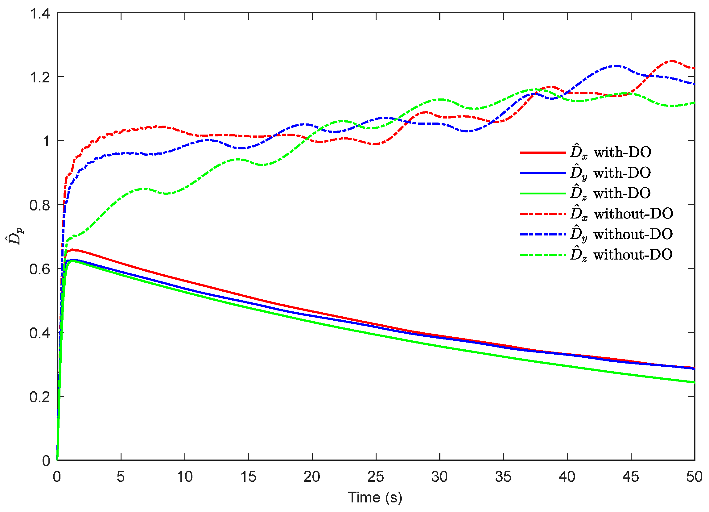Figure 7 shows the time evolution of the designed adaptive law, and it can be observed that the adaptive parameters of the position loop converge to a bounded constant after initial growth. When the adaptive law and the disturbance observer work together, the uncertainty compensation in the controller is assumed by the observer, the adaptive law plays an auxiliary role, and the adaptive parameter estimation is small. When the observer is removed, the adaptive law plays the main role, the estimated value is large, and obvious chattering phenomena may occur.

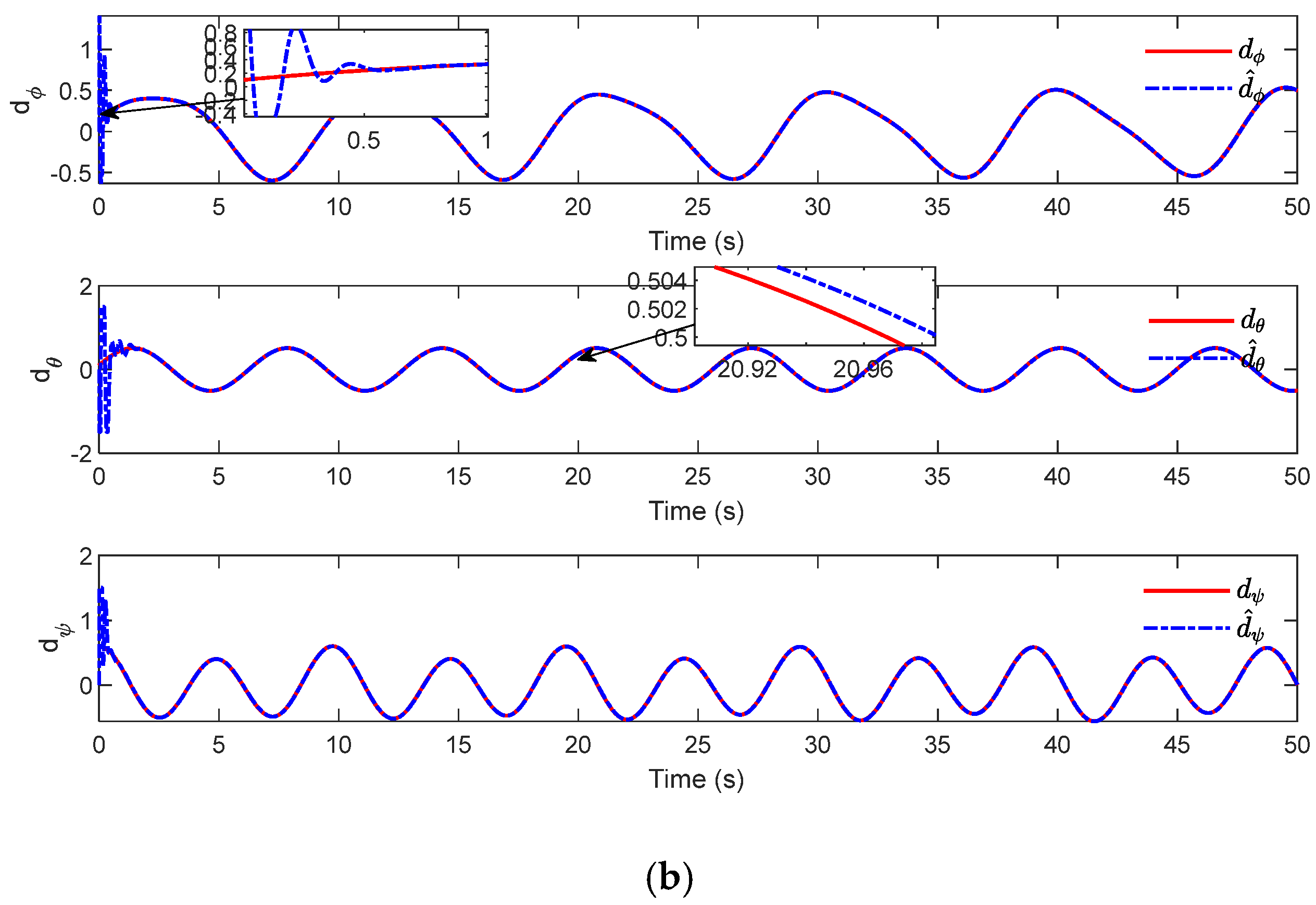
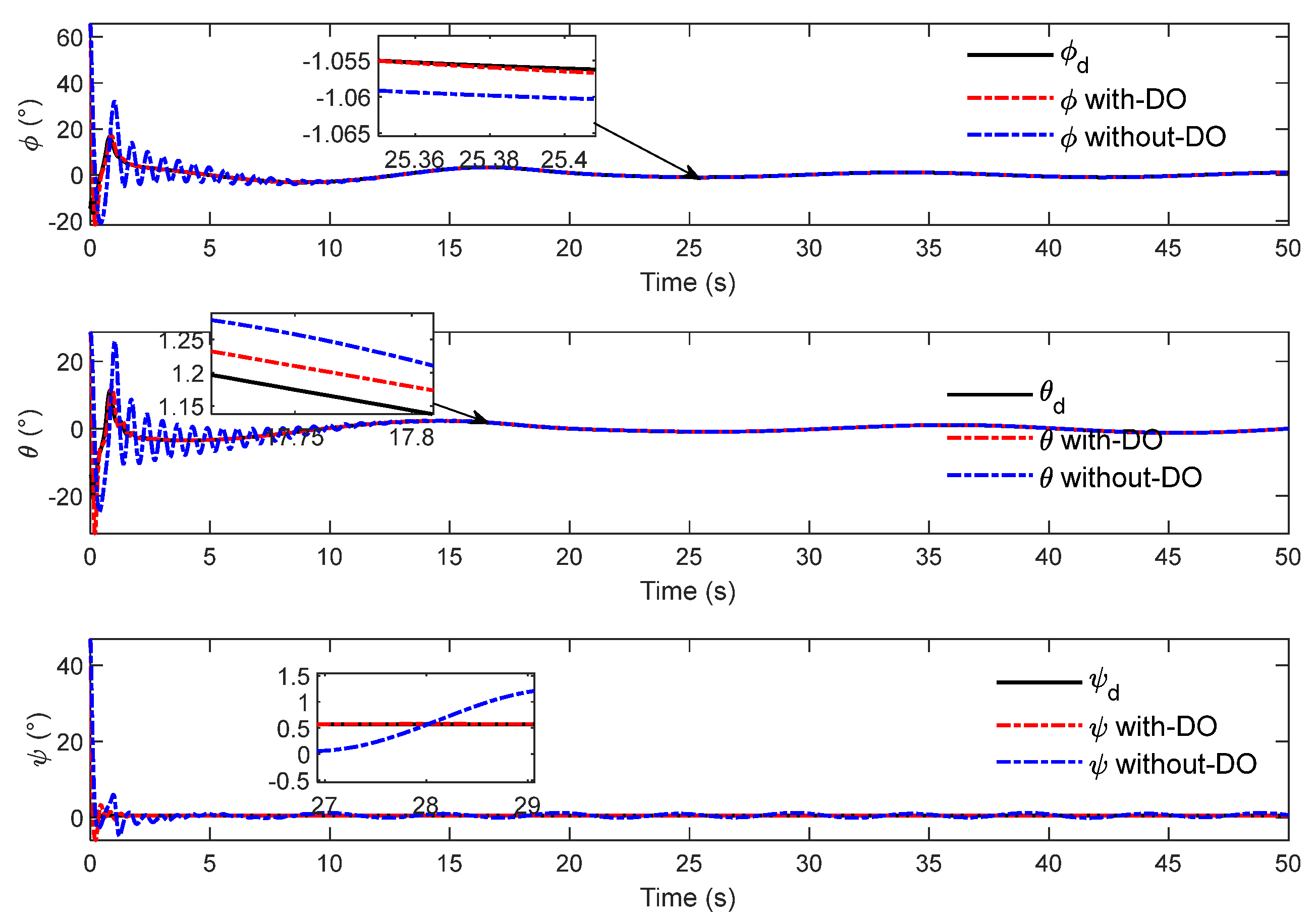
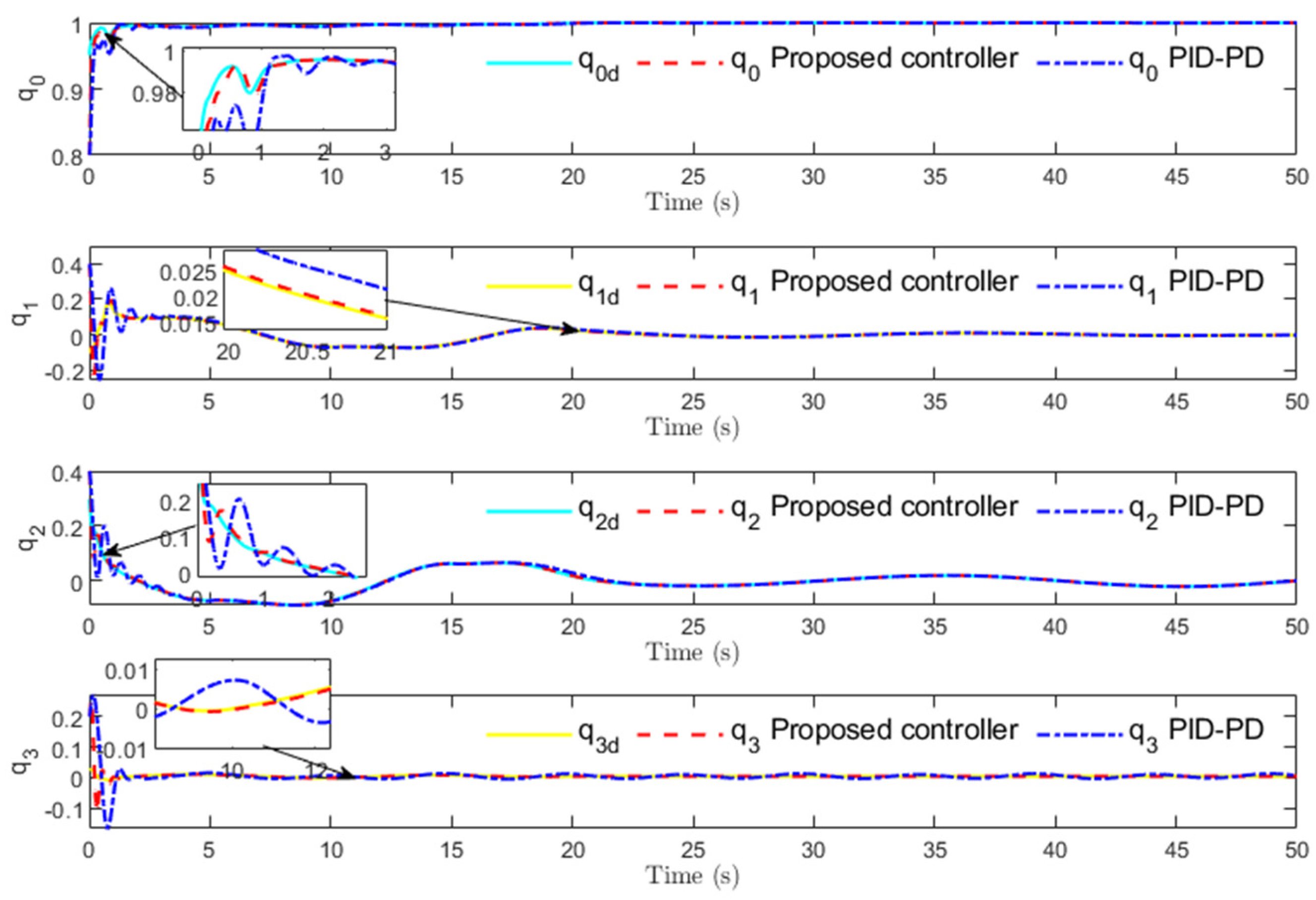
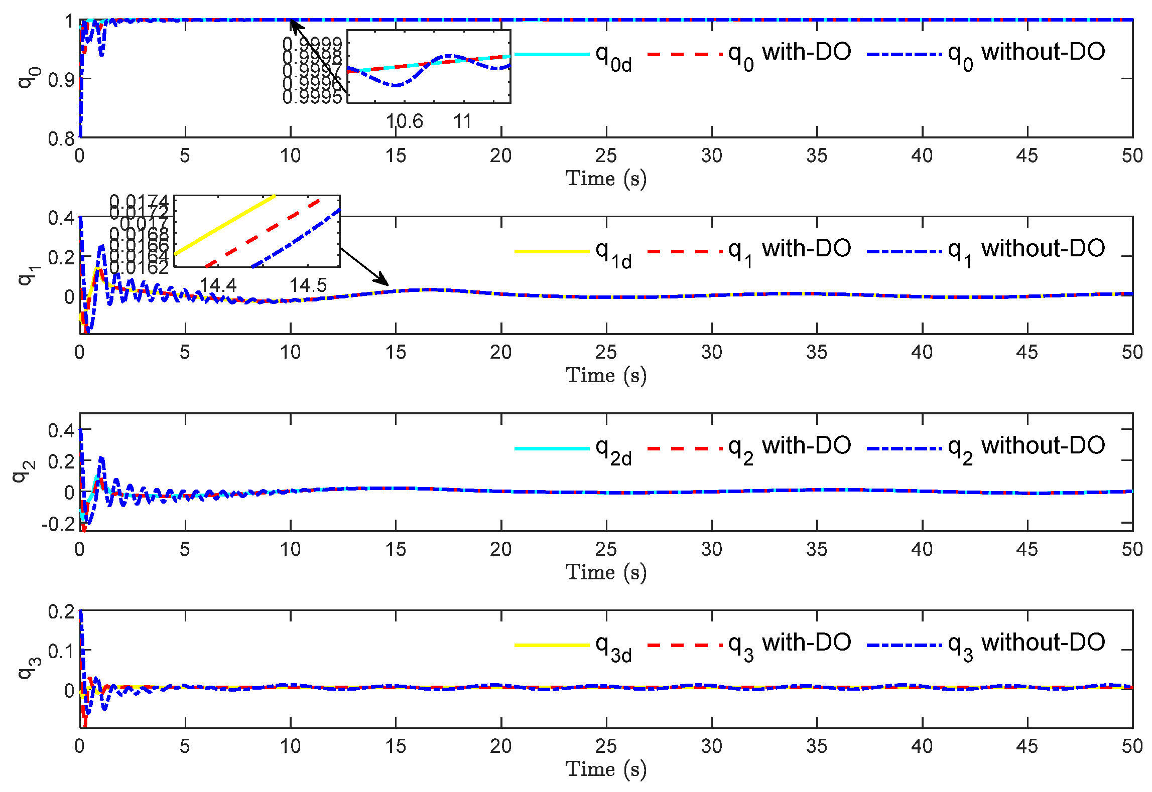
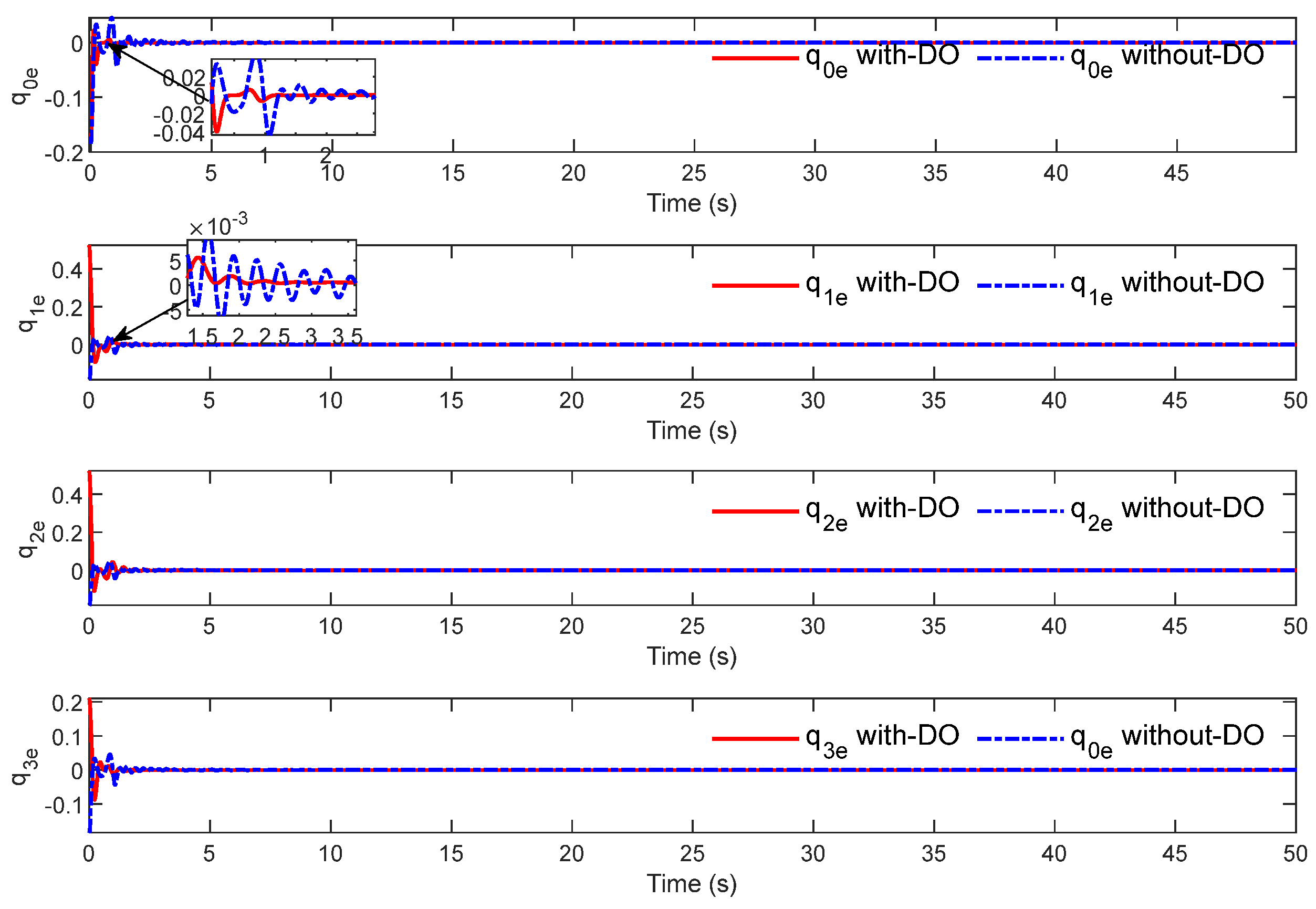
Figure 8 and Figure 9 show the attitude-tracking effect of the proposed inner loop controller. It can be observed in Figure 8 that the controller can drive the HAUV to accurately track the desired attitude angle. It can be seen in the locally enlarged image that the attitude angle tracking curve fluctuates more obviously under the action of the controller in reference [16]. Figure 9 shows that the four parameters of the quaternion can accurately track the expected quaternion value. 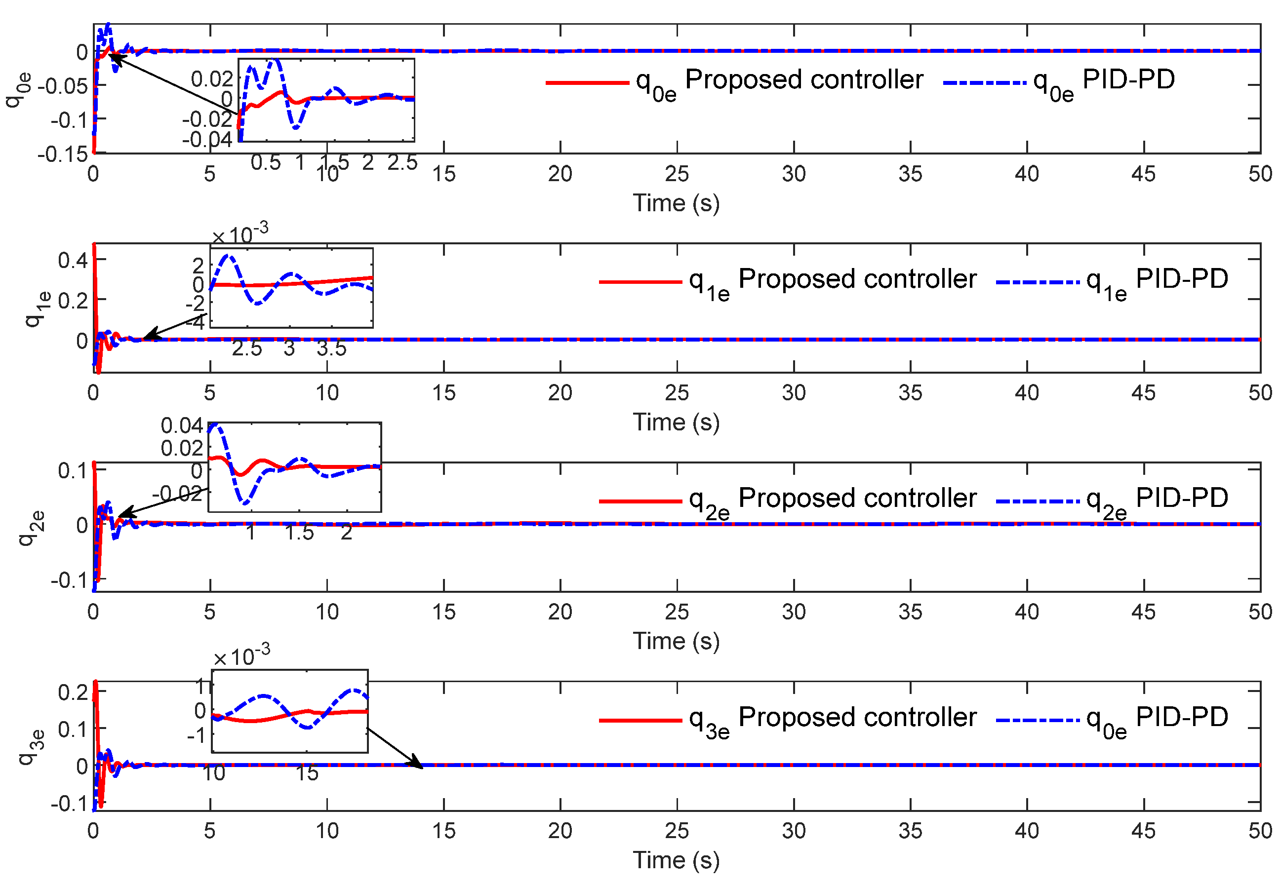Figure 10 shows the tracking error of the quaternion. When the inner loop subsystem is disturbed, the DO-enhanced quaternion PD controller can obtain a better tracking effect in both convergence speed and steady-state performance under the DO compensation effect.

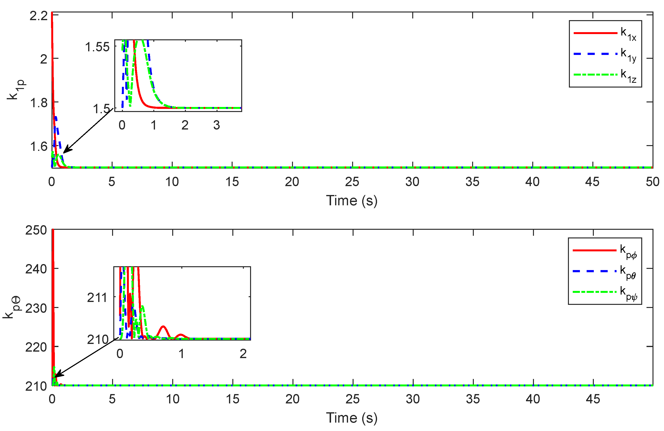
Figure 11 shows the evolution process of the learning rate parameter. It can be observed that the learning rate parameter increases rapidly in the initial stage, which is also the reason for the faster convergence rate of error. The analysis-based reason is that the error is the largest in the initial stage, and the error change rate is also large under the drive of the controller, which puts the learning rate parameter in a large state. With the rapid reduction in the control error, the learning rate parameter also rapidly decreases to the steady-state value, which indicates the excellent robustness and control accuracy of the controller from the side. Only when the error and error change rate are low does the learning rate parameter not experience large fluctuations. 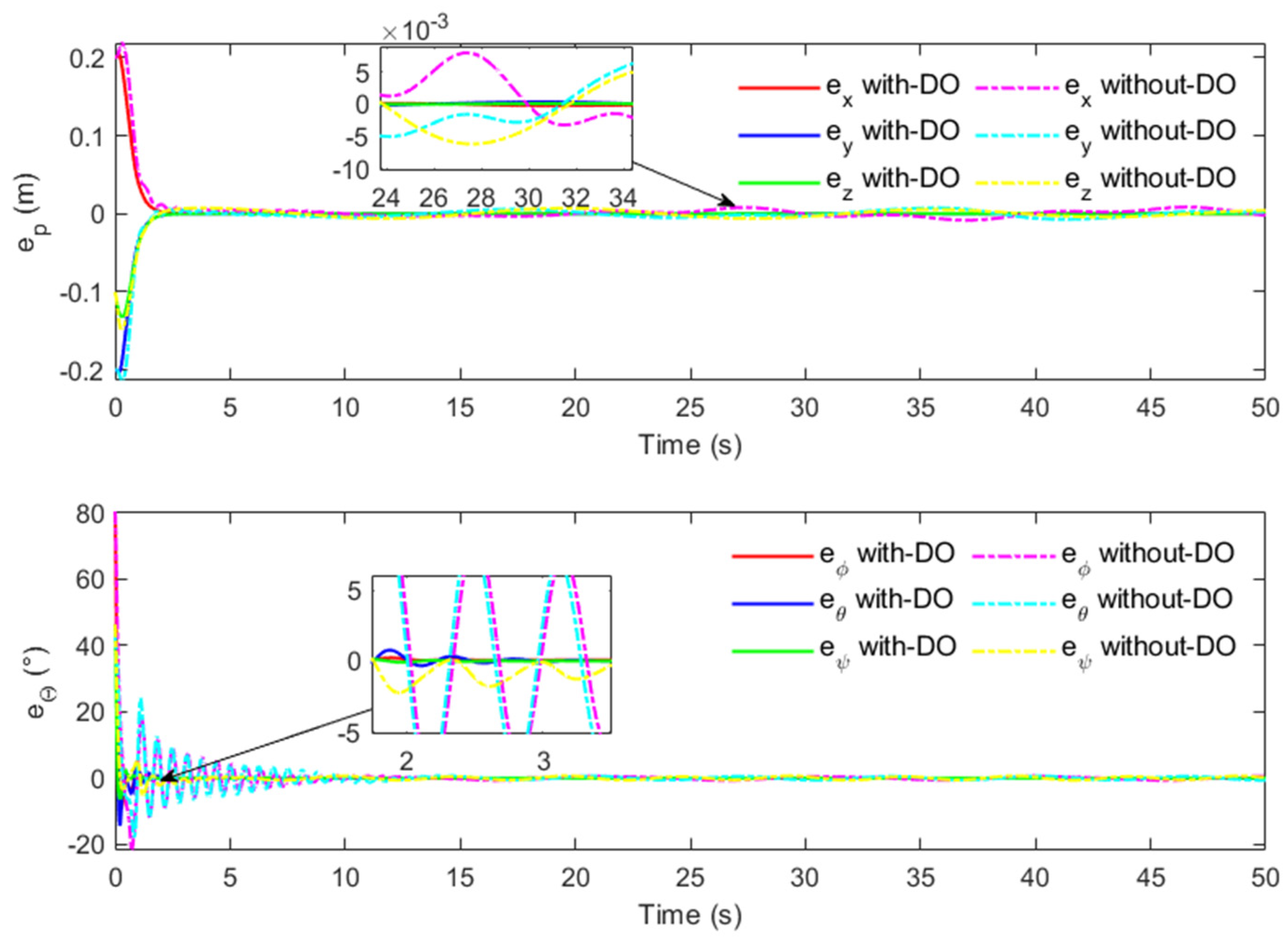Figure 12 shows the evolutionary effects of position and attitude-tracking errors. Obviously, the error of the position loop and the attitude loop converge near 0. This also shows that the controller that we designed has excellent robustness and low error fluctuation. However, [16] only adopts the classical linear controller, which lacks sufficient robustness, resulting in the control error always fluctuating greatly. 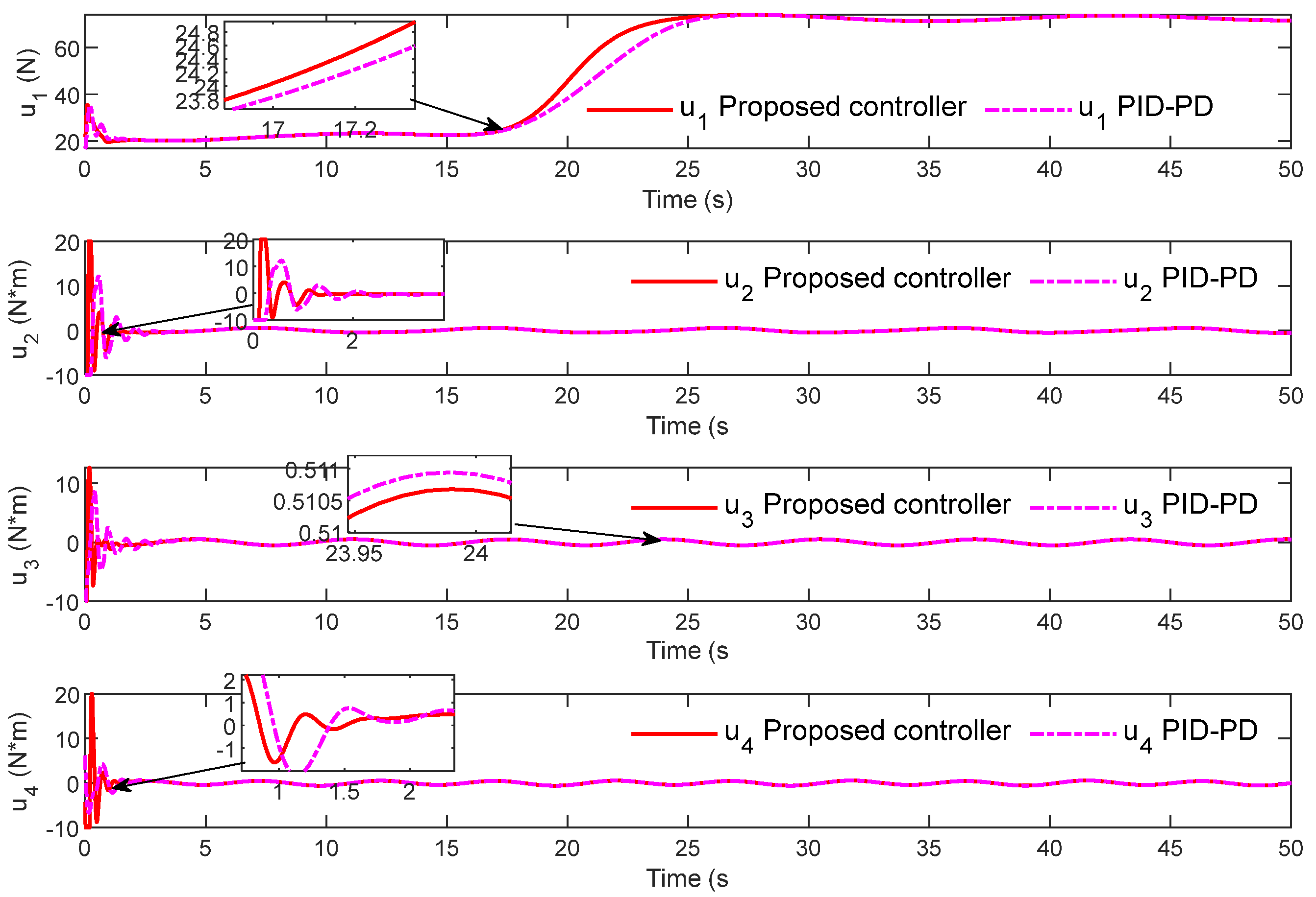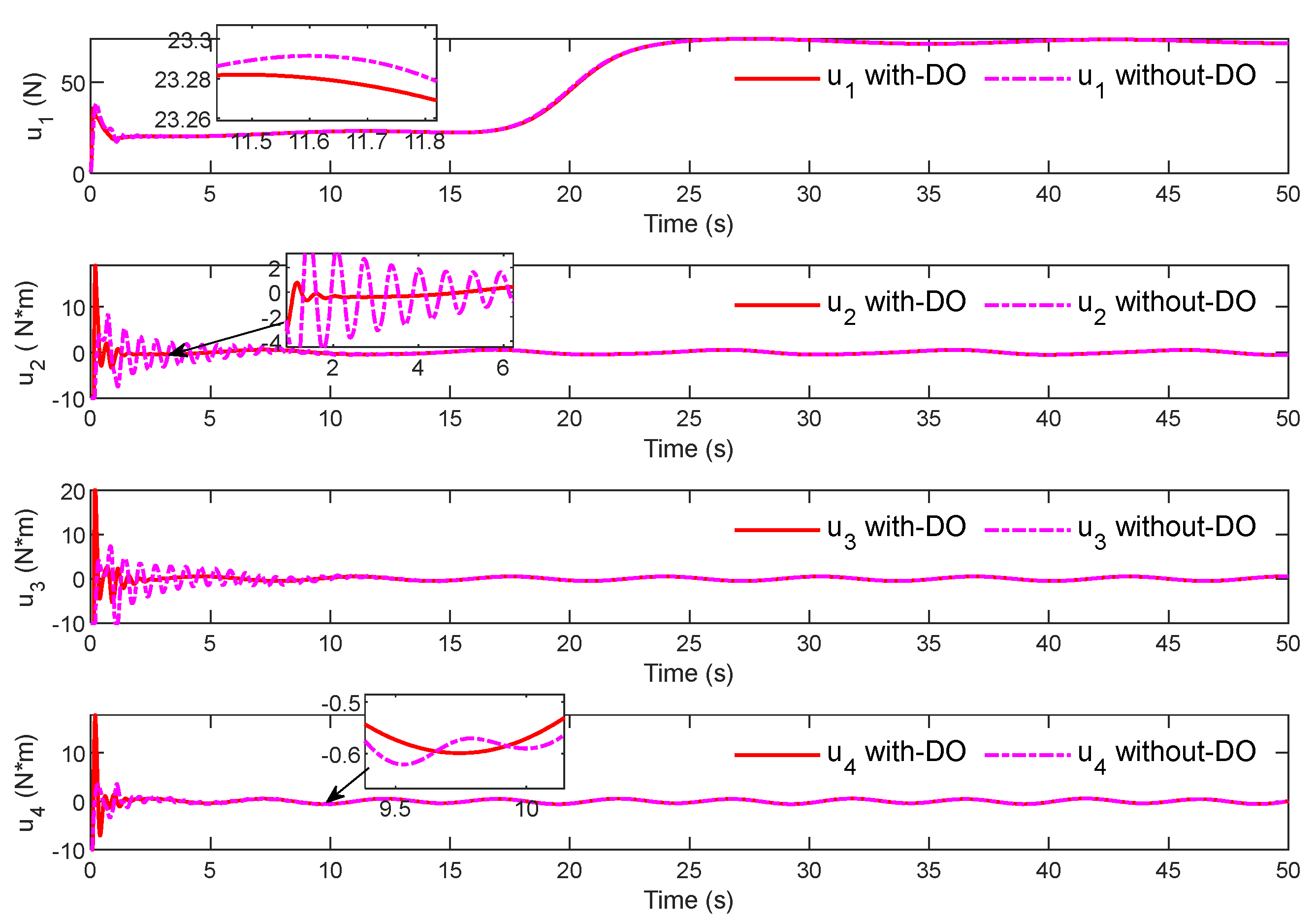Figure 13 shows the change process of the control signal. It can be seen that in the simulation process, the control signal variation trend calculated by the two controllers is similar. The first 20 s of the control inputs $u_1$ are obviously smaller than the last 30 s because the first stage is underwater maneuvering, where the HAUV achieves buoyancy compensation, and the lift output $u_1$ is small. In the latter stage, the HAUV enters the air from the water, the buoyancy disappears, and the total lift force has to overcome the influence of gravity, so the output value increases. Combined with the performance of the control error, the two controllers can change the output in real time according to the working state of the HAUV, but the proposed controller with superimposed DO obtains a more precise control signal.

4.2. Working Case 2 (Vertical Climbing Trajectory)

In the previous section, we tested the performance comparison between the designed controller and controller in [16]. The performance of the controller after the disturbance observer is removed is tested here, and other control parameters are the same as the controller designed in this paper. The trajectory of working case 2 is shown in the following equation. The vertical trajectory was chosen to test the ability of the coaxial HAUV to perform the fastest transmedium maneuvering in a disturbed environment.

$$\left\{\begin{array}{l}{x}_d=0\\ y_d=0\\ z_d=0.1t-2\\ {\phi }_d=0.01\end{array}\right.$$

(68)

Some simulation results for case 2 are provided in Figure 14, Figure 15, Figure 16, Figure 17, Figure 18, Figure 19, Figure 20, Figure 21, Figure 22 and Figure 23. Considering that the water surface of the real ocean environment is undulating, the spiral ascent under the wave water condition may cause the body to hit the wave and lead to the failure of take-off. Therefore, a cross-domain maneuver strategy of vertical climbing is adopted for condition 2. 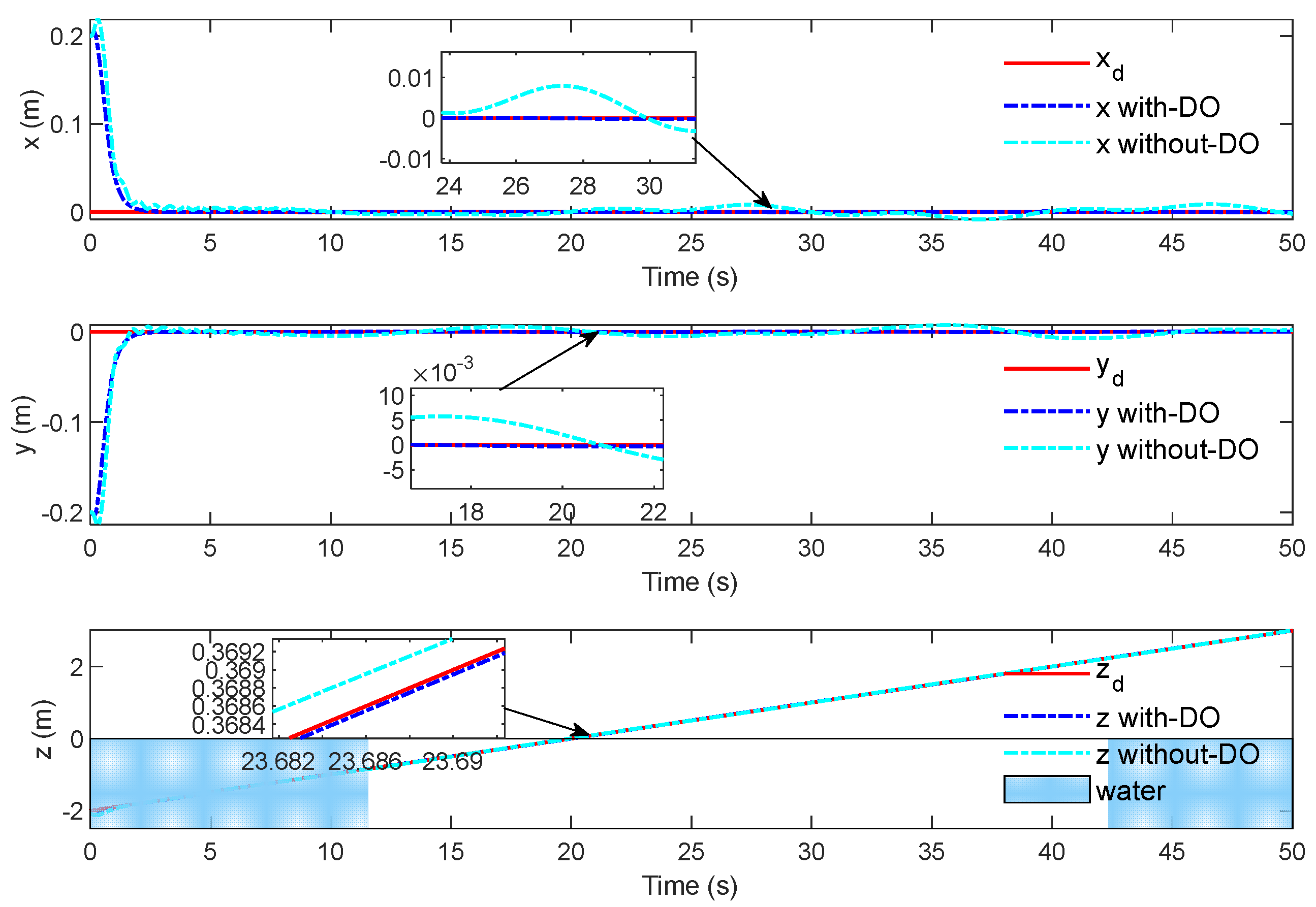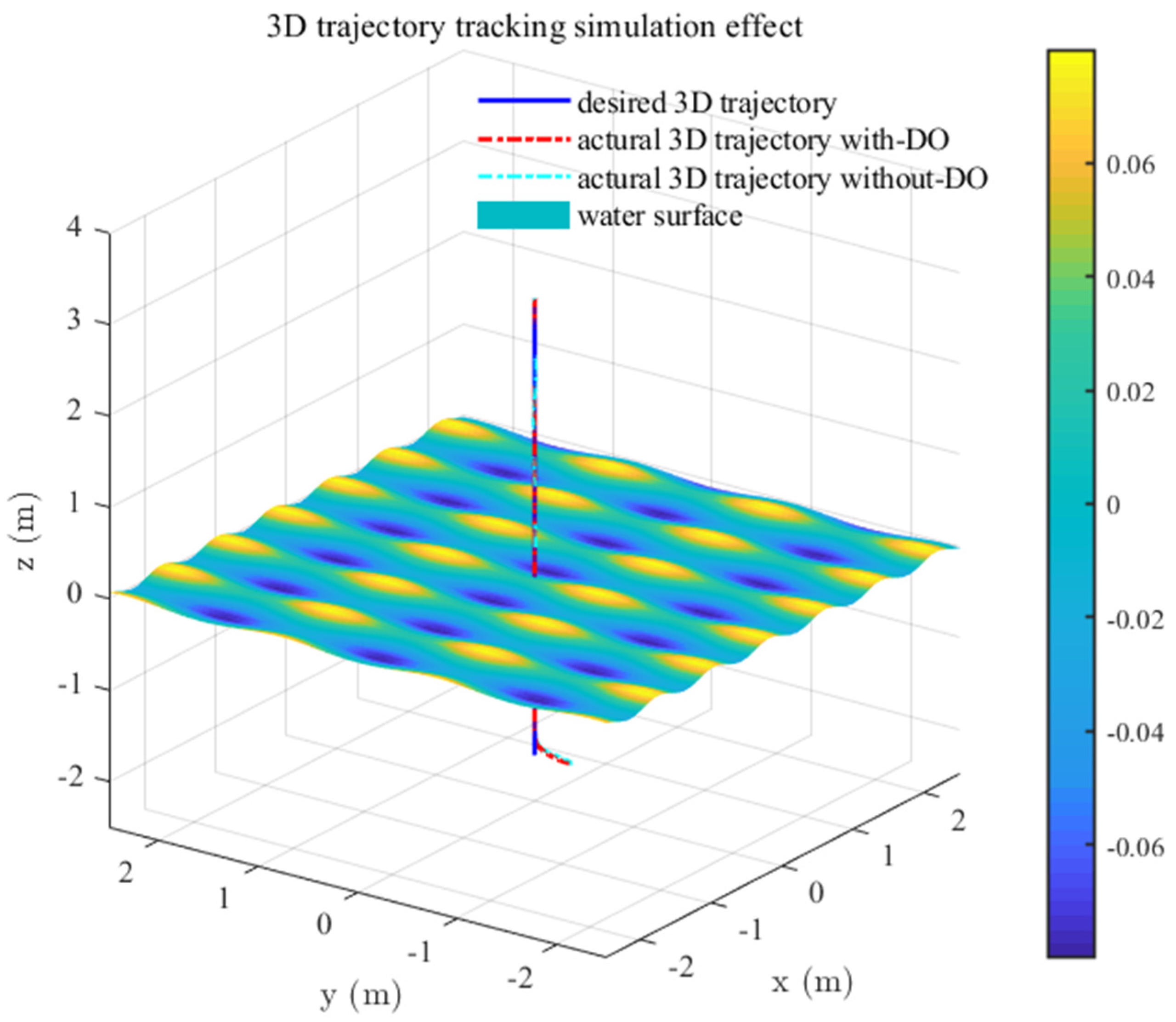Figure 14 shows the tracking evolution results of fixed-point climbing, which shows that the translation subsystem can still obtain better tracking results with DO enhancement. It can be seen in Figure 15 that the HAUV starts from underwater and passes through the wave surface vertically, showing a good 3D tracking effect. Figure 16 illustrates the rendering of the proposed observer for the unknown disturbance compared with the set value. In the results of disturbance estimation, the designed observer can quickly obtain the exact observation values. In particular, compared with the position loop, the observation value of the attitude loop observer fluctuates greatly in the initial stage. In future work, the optimal design should be carried out to avoid such situations. Figure 17 shows the time evolution results of the designed adaptive law, and the adaptive parameter estimates are stable and bounded. At the same time, the adaptive parameter values of the two controllers are obviously different, which means that the position controller adopted in this study can reduce chattering.

Figure 18 and Figure 19 show the attitude-tracking effect of the proposed inner loop controller; it can be observed that the HAUV tracks the desired Euler angle quickly, and the four parameters of the quaternions can accurately track the expected quaternions. At the same time, Figure 20 shows the tracking error of the quaternion and the fluctuation of the error in a small neighborhood of 0. The above results show that the controller based on observer enhancement technology can obtain a better tracking effect in both steady-state error and convergence characteristics.

Figure 21 shows the change process of the learning rate parameter under working case 2. In addition to the rapid increase in parameters in the initial stage, the learning rate parameters in the whole process are stable near the initial value, indicating that the control error of the controller is very small. Figure 22 shows the evolutionary effects of position and attitude-tracking errors. It is obvious that the controller with DO has better error convergence characteristics. Figure 23 shows the change process of the control signal after calculation. It can be seen that in the process of cross-media simulation, the changes in the four control inputs are stable and can be changed in real time according to the control target, and the control signal output of the adopted controller is more accurate.

In general, vertical cross-domain maneuvering is a more conservative and robust strategy, which can be realized with a small attitude change. The horizontal maneuvering ability can be abandoned in bad ocean conditions to prioritize the successful completion of cross-domain processes.

5. Conclusions

With the aim of solving the problem of the cross-media motion trajectory tracking of a coaxial HAUV under modeling uncertainties and external disturbances, an improved cascade SMC-PD control strategy is proposed to realize cross-domain motion. In the position loop, the composite robust controller was designed by combining the observer technique and the adaptive technique to meet the strong robustness requirements of the cross-domain process. On the other hand, the attitude error dynamics model of the HAUV was established by using the unit quaternion, which solves the singularity problem of the HAUV under large inclination maneuvers. In the cascaded control system, the inner loop controller needs a faster response speed, so a feedforward PD controller with a simple structure was adopted. The disturbance observer was added to the PD controller, which effectively enhanced its robustness. In addition, adaptive variable parameter technology based on the learning rate was introduced to the controller design process, which further improved the response speed of the controller. The Lyapunov theory was used to provide a rigorous proof of the stability of the closed-loop system. Finally, two typical cross-domain maneuverability strategies were simulated. By comparing the simulation results, the effectiveness and superiority of the proposed method for coaxial HAUV cross-media motion control under oceanic disturbances were verified.

In our future work, we plan to apply this proposed composite control to a real cross-domain platform to evaluate the algorithm’s performance through physical experiments. At the same time, new intelligence algorithms will continue to be developed.