Article

Multiscale Time Series Modeling in Energy Demand Prediction: A CWT-Aided Hybrid Model

by
Elif Sezer
1,*,
Güngör Yıldırım
2 and
Mahmut Temel Özdemir
3
1
Department of Electrical and Electronics Engineering, Munzur University, 62000 Tunceli, Türkiye
2
Department of Computer Engineering, Fırat University, 23100 Elazığ, Türkiye
3
Department of Electrical and Electronics Engineering, Fırat University, 23100 Elazığ, Türkiye
*
Author to whom correspondence should be addressed.
Appl. Sci. 2025, 15(19), 10801; https://doi.org/10.3390/app151910801
Submission received: 15 September 2025 / Revised: 2 October 2025 / Accepted: 5 October 2025 / Published: 8 October 2025
(This article belongs to the Topic Solar and Wind Power and Energy Forecasting, 2nd Edition)

Abstract

In the contemporary energy landscape, the increasing demand for electricity and the inherent uncertainties associated with the integration of renewable resources have rendered the accurate and reliable forecasting of short- and long-term demand imperative. Energy demand forecasting, fundamentally a time series problem, can be inherently complex, nonlinear, and multi-scale. Therefore, interest in artificial intelligence–based methods that provide high performance for short- and long-term forecasting, rather than traditional methods, has increased in order to solve these problems. In this study, a hybrid artificial intelligence model based on LSTM, GRU, and Random Forest, utilizing a distinct mechanism to address these types of problems, is proposed. The Multi-Scale Sliding Window (MSSW) approach was utilized for the model’s input data to capture the dynamics of the time series at different scales. The optimization of windows was conducted using the Continuous Wavelet Transform (CWT) method to determine the optimal window sizes within the MSSW structure in a data-driven manner. Experimental studies on Panama’s real energy demand data from 2015 to 2020 show that the CWT-aided MSSW-hybrid model forecasts better with lower error rates (0.007 MAE, 0.009 RMSE, 1.051% MAPE) than single models and manually determined window sizes. The results of the study demonstrate the importance of hybrid structures and window optimization in energy demand forecasting.

1. Introduction

Electrical energy, an indispensable infrastructure component of modern societies today, is critical for economic development and improving the quality of life. The sustainability of these impacts is directly related to the infrastructural adequacy of electricity grids and the availability of uninterrupted energy access. The global demand for electrical energy is on the rise, driven by an increase in consumption for both residential and commercial purposes. However, due to inadequate electricity generation, the supply–demand balance is deteriorating on a daily basis. This complicates the ability of electricity producers, distributors, and suppliers to effectively plan their energy use. For instance, when demand exceeds supply, operational problems such as voltage drops and unplanned power outages emerge within the system [1]. Conversely, when supply exceeds demand, problems such as inefficient resource use and increased production costs arise [2]. In both scenarios, the system’s stability is compromised. Especially today, as renewable energy sources become increasingly important, the imbalance between energy supply and demand has become an even more significant problem due to production fluctuations. Therefore, accurate energy demand forecasting ensures optimal energy production planning, maintaining the supply–demand balance. This allows for the sustainability of energy systems by reducing both economic losses and mitigating the impact of environmental factors. Moreover, energy demand forecasting, a fundamental element in power system design and development, is crucial from both a technical and financial perspective, as it improves power system performance, reliability, security, and stability while also reducing operating costs [3].
Forecasting energy demand has always been crucial in developing and managing energy policies. Therefore, many different approaches have been developed to solve energy demand forecasting problems. A systematic review of the extant literature reveals that these approaches can be categorized under five main headings: traditional statistical methods, machine learning (ML)-based methods, deep learning (DL)-based methods, hybrid models, and optimized hybrid methods. Traditional statistical methods (e.g., ARIMA, SARIMA), which use mathematical models based on past observations, operate on the assumption that the data structure is linear, making them inadequate in the face of complex patterns and external influences [4]. Therefore, machine learning (ML) algorithms (e.g., SVR, RF, XGBoost) capable of learning nonlinear relationships over time have been developed [5]. While these algorithms have exhibited robust performance on data augmented with external influences due to their flexibility, their inability to directly model time dependencies has constituted a substantial limitation. Deep learning (DL) models have emerged with their ability to capture long-term dependencies, seasonal changes, and sudden fluctuations in high-dimensional and complex data; structures such as Long Short-Term Memory (LSTM), Gated Recurrent Unit (GRU), and Convolutional Neural Network (CNN) have been frequently preferred in this context [6]. While each standalone DL model offers strong performance in certain scenarios, their generalizability to diverse data patterns is limited. Over time, there has been a growing trend toward hybrid models, which combine these architectures to leverage the strengths of each, providing more balanced and comprehensive learning. These models distinguish because they produce more accurate predictions by more comprehensively modeling both structural relationships and temporal patterns, and because they enhance the model’s capability to manage complex data structures. Another approach that has recently gained prominence in the literature is hybrid and optimization-assisted model structures, which aim to optimize model selection processes and hyperparameter tuning [7]. These models offset the weaknesses of individual models and provide solutions that are more aligned with the dynamic and multidimensional nature of energy demand forecasting.
As these methods are predicated on the forecasting of time series, their functionality is contingent upon the presence of patterns within the dataset. Extracting these patterns is a crucial step affecting model performance. The methods presented in the literature perform this intuitively, manually based on experience, or statistically. However, the efficacy of these methods is contingent upon the simplicity and size of the dataset. In the case of complex and extensive datasets, these methods may prove to be inadequate. To address this shortcoming, this study proposes a hybrid ML/DL-based energy estimation model that optimally executes the pattern detection process. Unlike other methods in the literature, the proposed model utilizes the Continuous Wavelet Transform (CWT) technique for pattern detection and utilizes a unique mechanism for prediction, employing LSTM, GRU, and Random Forest (RF) algorithms. Thus, a robust model has been proposed, integrating the long-term memory capacity of LSTM with the processing efficiency of GRU. The CWT mechanism also provides the model with Multi-Scale Sliding Window (MSSW) capability. The LSTM-GRU structure improves prediction accuracy, particularly in fluctuating, noisy, or irregular time series, and provides a more comprehensive temporal representation compared to other DL-based models. The Random Forest unit was integrated into the LSTM-GRU hybrid model to address the overfitting tendency of DL models and to achieve more stable and interpretable results with the final decision mechanism. The transformation of the complex temporal representations generated by the LSTM-GRU hybrid model into the final decision using Random Forest has been demonstrated to enhance the model’s generalizability and statistically improve its predictive success [8]. The efficacy of the model has been demonstrated through a comparative analysis of the results obtained from well-known classical ML and DL methods on the Panama dataset. Panama offers a particularly challenging case study for short-term load forecasting due to its climatic diversity, high dependence on hydro resources, and exposure to sudden demand shocks, including El Niño episodes and tourism-driven fluctuations. In summary, the contributions of this study to the existing literature are enumerated below.
  • Offering a different hybrid model to simulate real-world electrical energy supply and demand developments;
  • MSSW mechanism utilizing the Continuous Wavelet Transform technique for optimal extraction of time series patterns;
  • Enhancing forecast accuracy in noisy or irregular time series;
  • Incorporating the Random Forest algorithm into the model to circumvent potential overfitting issues when employing LSTM and GRU models in conjunction;
  • The model’s capacity to generate precise forecasts, even during periods of peak and valley demand.
The remainder of the paper is organized as follows: Section 2 provides a literature review of energy demand forecasting methods, while Section 3 addresses data analysis and problem definition. The technical specifications of the proposed model are delineated in this section. Section 4 elucidates the experimental methodology employed in conjunction with the proposed model, in addition to the comparative outcomes of these experiments. The conclusions and associated discussions are detailed in Section 5.

2. Related Works and Research Questions

Energy demand forecasting has been a subject of considerable interest in the energy sector and the relevant literature for many years. A plethora of different approaches exist for this purpose. For instance, Lin et al. proposed a Dual-Stage Attention-Based Long Short-Term Memory (DA-QLSTM) network for short-term electric load prediction in their study [9]. The initial stage of this model consists of a feature attention-based encoder that calculates the correlation of input features with the electric load and selects the most relevant inputs, while the subsequent stage consists of a temporal attention-based decoder that discovers temporal dependencies and selects the relevant encoder hidden states at all time steps. This model integrates the attention results with an LSTM model to derive probabilistic estimates through the application of a pinball loss function. This paper is noteworthy for its incorporation of an attention mechanism; however, the utilization of fixed time intervals in the model presents a problem of not capturing short-term seasonality.
Aouad et al. reported that their CNN-Seq2Seq-Att hybrid model, which combines a CNN, an LSTM-based Sequence-to-Sequence (Seq2Seq) network, and an attention mechanism, better captured peak values using a 60 h sliding window for short-term load forecasting of individual residential buildings in France [10]. In the model, the CNN extracted spatial information about the different variables affecting load consumption, while the Seq2Seq network extracted temporal dependencies from time-series data. The attention mechanism made the network more sensitive to peak consumption values and varying patterns in the electricity load data. However, due to the model’s complexity, computational costs are substantial, and external factors are disregarded. Ibrahim et al. conducted extensive experiments on the power system in Panama, integrating weather and holiday effects into their models and using various machine learning and deep learning methodologies [11]. However, although they used multi-layer deep learning models in their study, they skipped hyperparameter optimization. Joy et al. incorporated experimental hyperparameter optimization into their study, in which they proposed a multi-population differential evolution (DE)-based neural network embedded with a micro-genetic algorithm (mGA) to optimize short-term load forecasting (STLF) neural network (NN) models in Panama [12]. Multi-population DE is used to optimize the NN weights, and the diversity-preserving strategy of mGA is used to reduce premature convergence and diversify populations. However, due to the high computational cost of Multi-population DE, it is not suitable for real-time applications.
In their study, Sun et al. proposed MetaREC_LSTM, a data-driven metaheuristic method based on LSTM networks and an improved sine cosine algorithm (SCA) for STLF in Zhejiang, China. This method automatically tunes LSTM hyperparameters using SCA [13]. MetaREC employs the logistic chaos operator and a multilevel modulation factor to address the tendency of traditional SCAs to converge to local optima. It optimizes LSTM parameters, overcoming the uncertainty in LSTM prediction accuracy associated with manually selecting parameters such as the learning rate, the number of training sessions, and the number of neurons in the first and second layers. However, in their study, the model architecture (number of layers, activation functions) was not optimized, and normalization/missing data filling processes remained unclear. In this regard, Shohan et al. proposed a hybrid prediction method that combines LSTM and neural prophet (NP) networks via artificial neural network (ANN) and dynamically adjusted the number of layers and neurons in their model [14]. This study presents multiple case studies for three different types of load forecasts -hourly, daily, and annual- using two different datasets in the US. Missing data is filled in using min-max normalization, linear interpolation, and seasonal averaging. However, the Levenberg–Marquardt (LM) algorithm used in ANN requires high memory requirements and has poor NP performance for long-term forecasts. In their study, Navarro Valencia and Sanchez-Galan employed a Temporal Fusion Transformer (TFT), an attention-based neural network model, for the STLF in Panama. This approach addresses the limitations of NP in long-term predictions by utilizing a multi-head attention mechanism architecture [15]. In contrast to the NP model, this model exhibits high performance, even for predictions made 30 days in advance, by employing LSTM units and multi-head attention mechanisms. However, TFT’s high training time and computational cost present significant disadvantages in practical applications.
Mobarak Abumohsen et al. employed LSTM, GRU, and Recurrent Neural Networks (RNN) in their study to forecast the electricity load in Palestine, achieving a comparable level of accuracy with the lighter architecture of GRU [16]. These models were tuned using seven different types of hyperparameters, including optimizer, activation function, learning rate, epoch count, batch size, hidden layer count, and dropout. However, the specifics of the data preprocessing procedures are unclear in the study. In their study, Mounir et al. proposed EMD-BI-LSTM, a hybrid method based on Empirical Mode Decomposition (EMD) and Bidirectional LSTM (BI-LSTM) for STLF and performed data preprocessing with EMD [17]. The EMD method decomposes a time series into a set of stationary components, known as Intrinsic Mode Functions (IMFs). The BI-LSTM model is employed to estimate each IMF, considering both past and future data. The component estimates are then combined to yield the overall forecast. The temporal resolution of the IMFs captures short- and long-term patterns without the need for SW; however, a salient disadvantage of this approach in STLF is its high computational expense. Farsi et al. employed a novel hybrid deep learning model dubbed the Parallel LSTM-CNN (PLCNet), for the analysis of STLF in Malaysia and Germany, reducing the computational burden by extracting features directly with CNN without EMD [18]. This study, which aims to make predictions without the need for exogenous variables and uses PLCNet, CNN, and LSTM in parallel, uses the CNN to utilize for the extract input data features, while the LSTM to learn long-term dependencies within the data. Subsequent to the combination of the outputs, a fully connected path combined with an LSTM layer is utilized to produce the final prediction. The model’s performance is low in long-term predictions, and its capacity to address seasonality is deficient. Additionally, the study performed a 24 h forecast by looking back over 72 h; however, the window size was not subjected to analysis.
In a recent study, Ullah et al. proposed a hybrid CNN-LSTM model for STLF in Pakistan and conducted a comparative analysis of window sizes ranging 24.72 and 168 h [19]. This model utilizes CNNs for the extraction of features from high-dimensional data and LSTM networks for the prediction of temporal sequences. The model architecture is designed to process sequential data with 24 time steps and 17 features per time step. Despite the shortcomings of feature selection in Ullah et al.’s study, Khalid Ijaz et al. proposed a new temporal feature selection-based ANN-LSTM model for STLF in Malaysia. This model provides a combination of a standard ANN and sequential LSTM cells, using an ANN-based feature selection method [20]. The objective of this study is to address the challenges posed by overfitting and underfitting, with the aim of accurately capturing the nonlinear patterns exhibited by electric load curves. The ANN layer is responsible for extracting significant temporal characteristics. The feature matrix, which is extracted by this layer, is subsequently input into the LSTM cell for estimation. However, the impracticality of implementing fixed-time-delay LSTM models and the lack of a sliding window in temporal data can lead to short-term seasonality capture problems. Rafi et al. proposed a CNN-LSTM hybrid model for the STLF in Bangladesh, reframing the data with 7-day time steps and thus better modeling seasonality [21]. The CNN block of the model is designed to extract latent features, while the LSTM module is designed to learn long-term dependencies of the load dataset. However, the model has only been evaluated for its short-term (1 week) prediction capabilities. In their study, Chen et al. address the challenges posed by load volatility and the difficulty in tuning the algorithm parameters [22]. They propose a hybrid model, namely the CEEMDAN-IGWO-GRU (CIG) hybrid algorithm, which combines full ensemble empirical mode decomposition with adaptive noise (CEEMDAN) for STLF, an improved gray wolf optimizer (IGWO), and a GRU. In this study, the impact of load volatility is mitigated by CEEMDAN–Permutation Entropy (PE), and the parameters of the GRU network are optimized using the IGWO. The evaluation process involves the meticulous analysis of Singapore’s electricity load data, yielding precise results. Nevertheless, the intricacy of this approach and the substantial computational demands resulting from its multi-stage configuration constitute limitations of the study.
Studies on Panama data are remarkable but have limitations. Attention-based approaches [15] focus on a single timescale and fail to adequately model short-term fluctuations and seasonal trends. DE optimization models [12] have advantages, but they remain at a fixed time resolution and fail to evaluate critical metrics. Traditional ML methods [11] are reasonable, but often lack validation on a second dataset or reproducibility.
Table 1 provides a detailed comparative summary of recent studies that have not been addressed in this section. As demonstrated in this synthesis, while prior efforts have exhibited significant advancements, they frequently exhibit inconsistencies in the treatment of multi-scale temporal patterns and wavelet-based feature engineering. These gaps underscore the impetus for the present study.
The present study is driven by three fundamental research inquiries:
  • How does the consideration of multi-scale temporal dependencies affect the accuracy of electricity demand forecasting?
  • To what extent does the integration of LSTM’s long-term memory capacity with GRU’s computational efficiency surpass the performance of classical ML and DL baselines?
  • Can the proposed model sustain its forecasting performance and demonstrate generalization ability when validated on an independent dataset?
In order to address the aforementioned inquiries, the objectives of the present study are threefold: first, to benchmark the proposed hybrid model against well-established ML and DL approaches using the Panama dataset; second, to perform ablation studies in order to evaluate the contribution of individual model components; and third, to assess the model’s generalization capability through cross-dataset validation on a secondary dataset.

3. Methodology

This section presents the developed methodology for energy demand forecasting and its steps in detail. The initial steps of the proposed methodology entail the analysis of the dataset and the selection of features. The subsequent stage involves the implementation of wavelet transform analysis, a distinctive component of the proposed methodology, which facilitates a more comprehensive examination of patterns in historical data and automates this process. Subsequently, a deep learning model was constructed and trained to forecast the data. This model employed a hybrid of LSTM, GRU, and random forest methods. The performance of the proposed method was evaluated using MAE, RMSE, and MAPE metrics and presented in comparison with other methods.

3.1. Dataset Used and Feature Selection

The study utilized a publicly accessible dataset [https://www.kaggle.com/datasets/ernestojaguilar/shortterm-electricity-load-forecasting-panama (accessed on 2 September 2025)] comprising real-time energy demand records for Panama, spanning the period from 2015 to 2020. The dataset also contains 16 separate attributes representing various weather parameters from three major Panamanian cities, along with ancillary information such as public holidays. A comprehensive overview of the dataset’s characteristics is provided in Table 2. This study focuses on the 48,048 hourly national load (nat_demand) data in this dataset. In order to gain insight into the characteristics of the dataset and the process of feature selection, a correlation heatmap for the dataset was first created using the Pearson Correlation technique. The correlation heatmap in Figure 1 reveals moderate positive correlations between the national load and the weather attributes in the dataset (T2M_toc, T2M_san, T2M_dav). No substantial correlations were identified with the remaining attributes.
Recent studies emphasize that digitalization and real-time forecasting approaches are increasingly designed for practical deployment, including hardware-based implementations [30]. The proposed model has been developed to address the critical needs of real-time electricity demand forecasting, where achieving both accuracy and computational efficiency is paramount. To ensure practical applicability in real-time environments, the model is constructed with the minimum number of relevant features. This reduction in dimensionality has been shown to decrease complexity, shorten computation times, and enhance generalizability, while still maintaining high predictive performance.

3.2. Electricity Demand Behavior Analysis

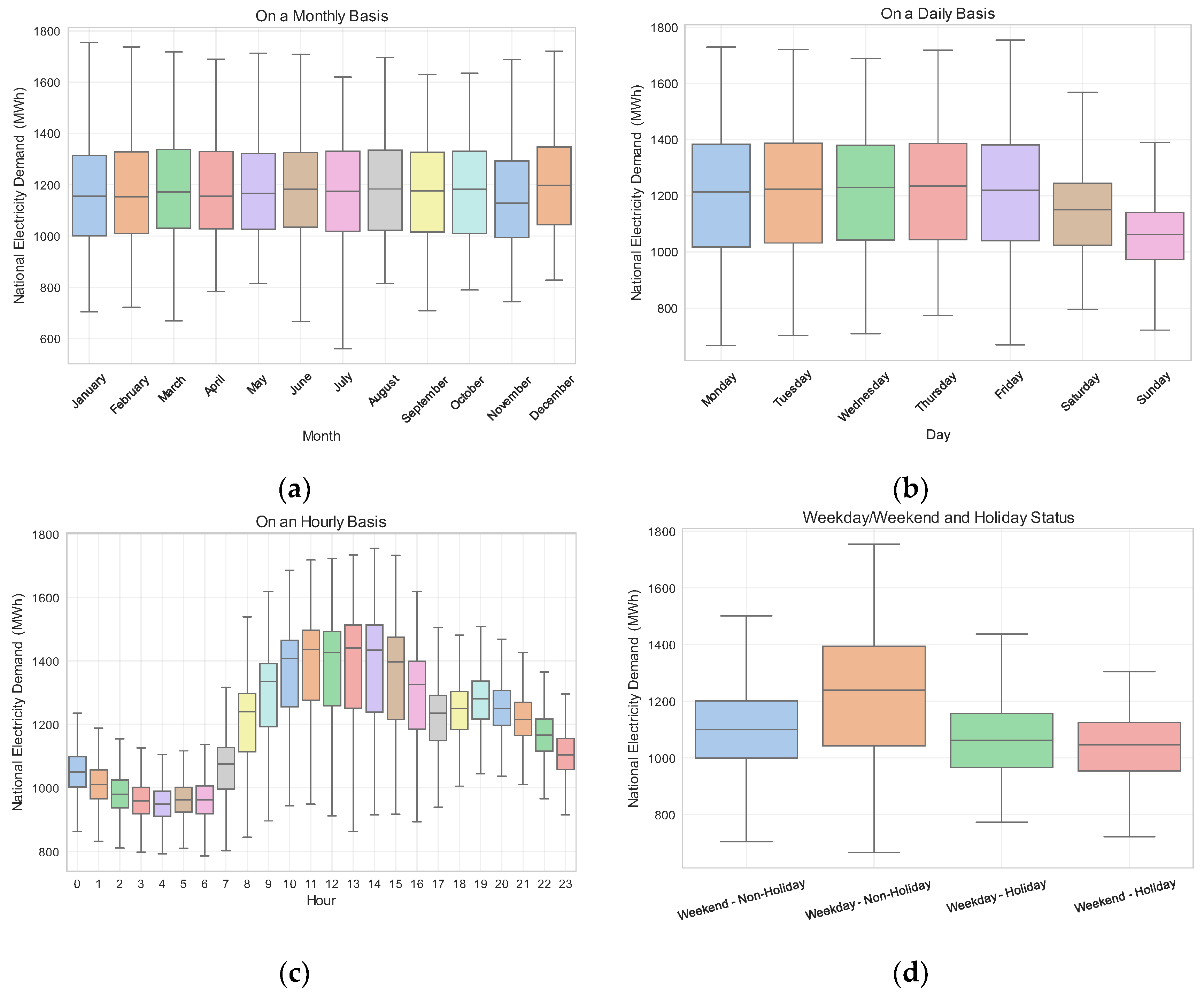
In order to achieve a more profound comprehension of peak energy demand periods, the monthly, daily, hourly, and weekend/holiday data distributions in Figure 2a–d can be examined. This enables the estimation of overload times for the implementation of preventive measures against overloading problems, and the identification of minimum load times to minimize network losses [16]. The IRQ graphs reveal that there are no significant differences between months, and the median values are relatively similar throughout the year. This finding indicates that energy demand is not substantially influenced by seasonal variations throughout the year and the system exhibits a greater sensitivity to daily and hourly rhythms. A daily analysis reveals that median values are elevated and consistent from Monday through Friday. In contrast, median and upper quartile values demonstrate a decline on Saturday and Sunday. This indicates that electricity demand is high on weekdays and low on weekends, suggesting a substantial impact from work and school activities. Demand is expected to be minimal between midnight and 6:00 AM, increase rapidly from 8:00 AM onward, reach its peak between 12:00 PM and 3:00 PM, and then decline again. This anticipated phenomenon is likewise observed in the energy demand during weekends and holidays. It is evident that demand exhibits a decline during holiday periods and a surge during weekdays.

3.3. Continuous Wavelet Transform

A primary strength of the proposed method is Continuous Wavelet Transform (CWT), a sophisticated technique employed in time-frequency analysis. Classical energy demand forecasting approaches in the literature employ time series pattern analysis manually, statistically, or empirically. This may result in failure to detect certain patterns in large datasets. Therefore, this study employed the CWT technique to capture intricate patterns that elude detection by conventional methods. CWT possesses the capability to visualize this process and furnish decision-makers with detailed results. CWT is a technique that provides both time and frequency information simultaneously by examining signals at different scales using different wavelet forms. CWT is a technique that provides both time and frequency information simultaneously by examining signals at different scales using different wavelet forms [31]. The primary signal is multiplied by a function known as a wavelet, which can be shifted in time and whose amplitude can be varied. The analysis is then continued by shifting the signal in a stepwise manner. At each step, coefficients representing the correlation between the wavelet function and the signal are calculated. These coefficients indicate how the similarity between the signal and the wavelet changes along the time axis. The analysis is repeated using wavelet functions at different scales. For each scale value, the wavelet coefficients are obtained as a function of time [32]. The mathematical expression demonstrating the CWT process and the associated parameters are as in Equation (1) [33] and Table 3.
C W T ( s , τ ) = 1 s x t . ψ s , τ * t τ s d t
As demonstrated by the equation, the process entails the multiplication of the signal by the wavelet function for each (s, τ) pair, followed by the integration of the result. This process enables the analysis of different frequency components and scales of the signal according to the scale factor of the wavelet.

3.4. Proposed Deep Learning-Based Prediction Model

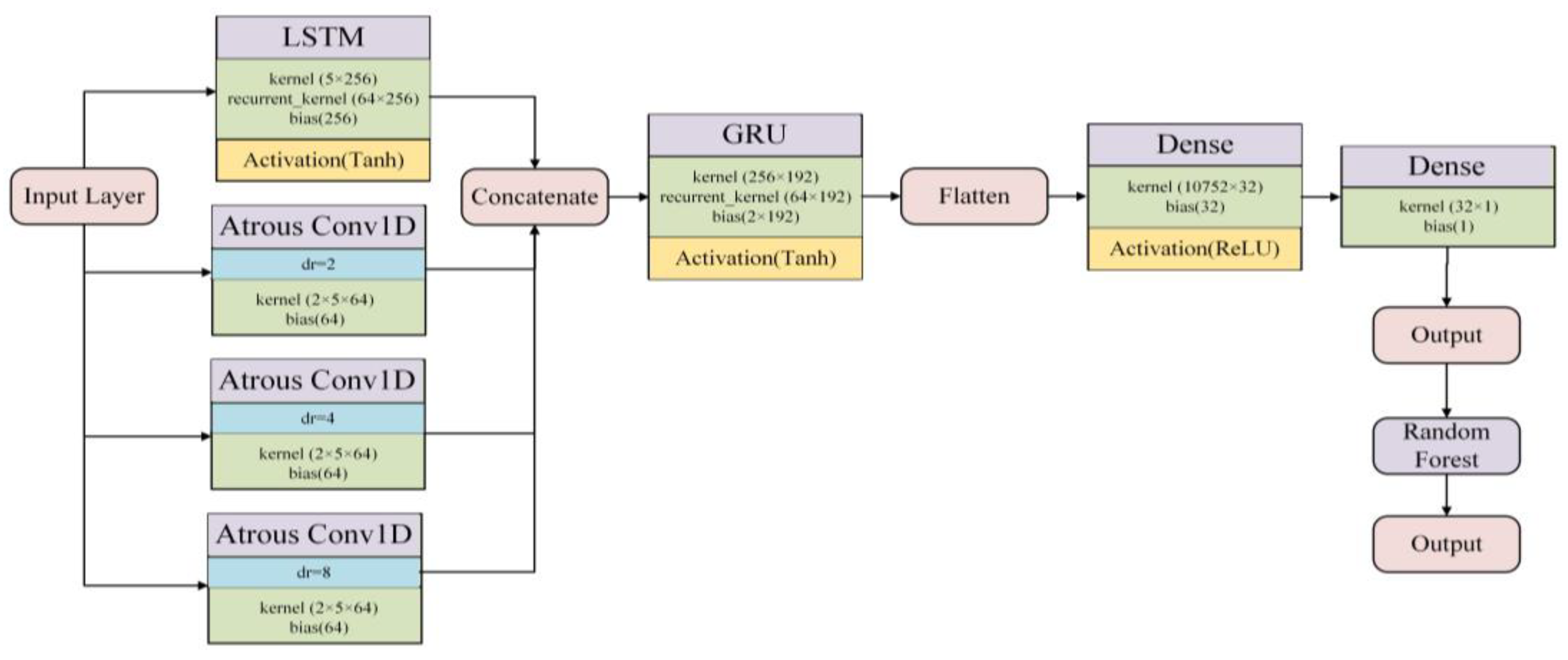
A critical component of predictive analysis is the model’s capacity to discern both short-term and long-term patterns. Classical methods can struggle to achieve the desired results, particularly in data spaces characterized by intricate relationships. Deep learning models, which have demonstrated considerable efficacy in recent years, are capable of capturing such complex relationships. However, deep models are also known to suffer from overfitting and interpretability issues. Classical tree-based methods have demonstrated greater efficacy in addressing these deficiencies. Consequently, for a critical problem like demand prediction, developing more flexible ensemble models instead of using deep learning or classical methods alone can improve performance. To this end, an ensemble model was obtained for the purposes of this study. This model includes layers of well-known deep learning models, LSTM, GRU, and Random Forest, which is a classical machine learning method. One-dimensional convolution layers were incorporated into the model to capture local patterns and suppress noise. While LSTM and GRU layers are capable of learning more complex temporal relationships, the representations obtained from these layers are transformed into interpretable and generalizable predictions by Random Forest. The overarching architecture and salient features of the components of the artificial intelligence (AI) model developed for demand forecasting are delineated in Figure 3 and Table 4. Descriptions of each subunit of the model are provided below.

3.4.1. Long Short-Term Memory Unit

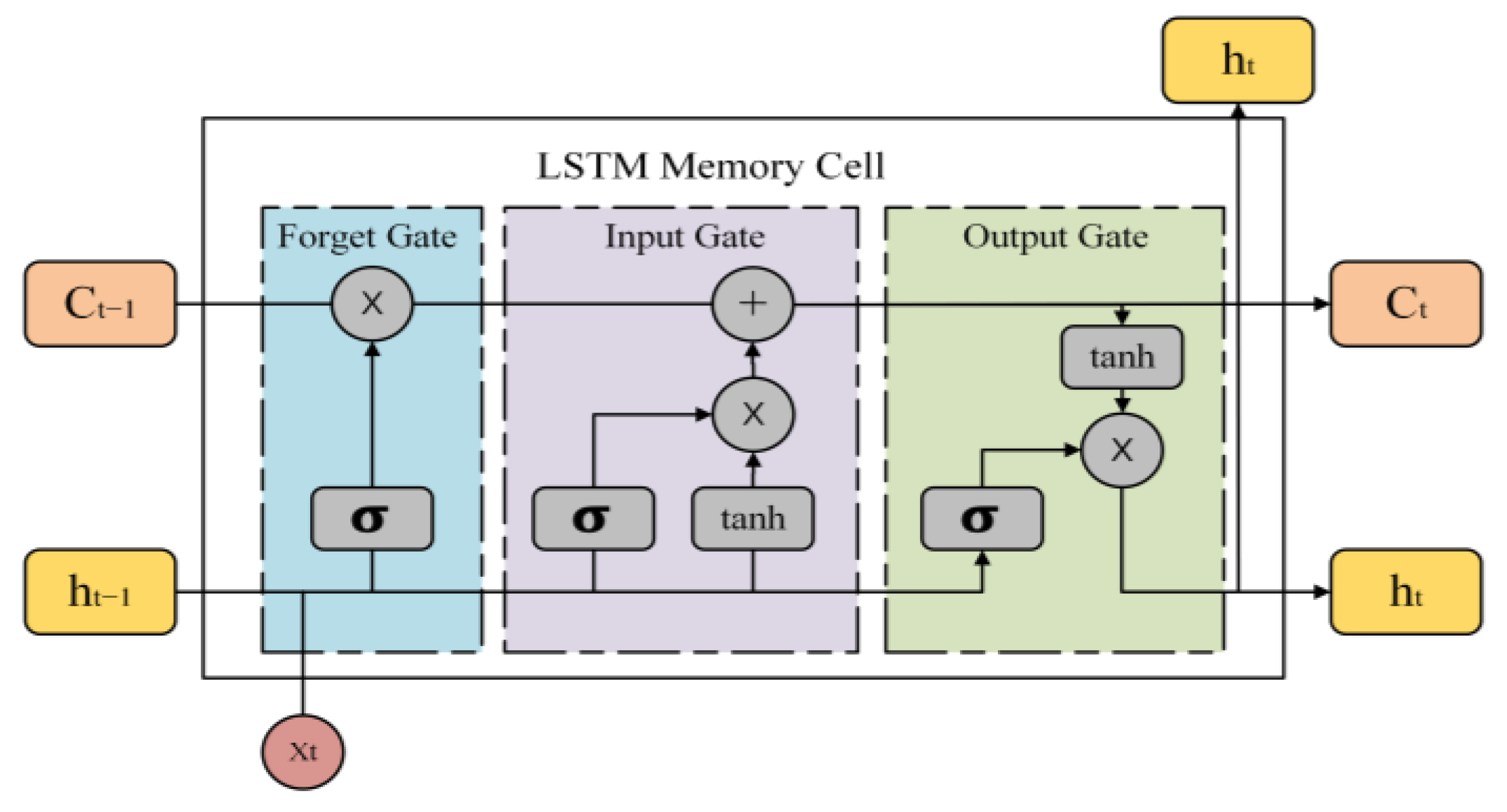
LSTM models are unique structures belonging to the recurrent neural network (RNN) family that overcome the vanishing gradient problem, a challenge often encountered in traditional RNNs [34]. In addressing forecasting challenges, those posed by time series, LSTM is notable for its long dependency and flexibility features. LSTM employs three gates—the forget gate, the input gate, and the output gate—in conjunction with a cell state to regulate information transfer. These gates collaborate to acquire and retain information regarding the long-term and short-term sequence in the LSTM cell and are structured to be backpropagated across time and layers [35]. The input gate is the gate that determines which information is to be added to the cell state from the input. The forget gate is responsible for retaining only the relevant information and determining what should be removed from the h t 1 state. The output gate is the gate that determines what information is to be output from the current cell state [36]. The general architecture of an LSTM is illustrated in Figure 4. The mathematical model of the working mechanisms of LSTMs described above and the details of the parameters used in this model are given in Equations (2a)–(2f) [37] and Table 5, respectively.
f t = σ W f · h t 1 , x t + b f
i t = σ W i · h t 1 , x t + b i
o t = σ W o · h t 1 , x t + b o
C ~ t = tanh W C · h t 1 , x t + b C
C t = f t C t 1 + i t C ~ t
h t = o t tanh C t

3.4.2. Gated Recurrent Unit

GRU, an RNN-based structure, is noteworthy for its simplicity and effectiveness in handling long-term dependencies, particularly in time series data [38]. Due to its relatively fewer training parameters as compared to the LSTM model, GRU is particularly well-suited for scenarios where resources are limited and training times are stringent [39]. GRU consists of gated layers analogous to LSTMs, yet it possesses a simpler structure [40]. The GRU cell utilizes two primary gates: the Update Gate and the Reset Gate. The update gate dictates the extent to which the preceding moment’s state information is retained in the current state, while the reset gate determines whether the current state is to be merged with the preceding information [41]. Increasing the value of the update gate means that more state information will be stored, and increasing the value of the reset gate means that more historical information will be preserved [42]. As illustrated in Figure 5, these mechanisms are implemented within a GRU model. The mathematical model and parameters of the GRU are delineated in Equations (3a)–(3d) and Table 6.
z t = σ   ( W z x t + U z h t 1 + b z )
r t = σ   ( W r x t + U r h t 1 + b r )
h t ~ = tanh ( W h x t + U h r t h t 1 + b h )
h t = 1 z t h t 1 + z t h t ~

3.4.3. Random Forest Model

The Random Forest model, which exhibits both high prediction accuracy and low variance, is a prominent ML model that involves the training of multiple decision trees and is utilized for both classification and regression problems [43]. A random forest model employs decision tree representing branches as input features and leaves as prediction results, and aims to predict the target outcome based on the features [44]. The random forest model offers strong generalization capabilities by evaluating the generalization error with an unbiased estimate. The model demonstrates resilience to outliers and efficiently calculates predictions in regression by utilizing the mean of trees [45]. A salient feature of random forest, the mathematical model and parameters of which are delineated in Equations (4a) and (4b) and Table 7, is their capacity to yield interpretable results through the if-else structure they facilitate [46].
f t x = 1 l t ( x ) i l t ( x ) y i
y ^ = 1 T t = 1 T f t ( x )  

4. Experimental Results

The proposed model was evaluated using Panama electricity energy demand data, a well-documented and widely recognized dataset in the relevant literature. The findings of the model tests were also examined in relation to the results of other prominent deep learning and machine learning algorithms, including LSTM, GRU, RNN, FNN (Feedforward Neural Network), SVR (Support Vector Regression), XgBoost (Extreme Gradient Boosting), and KNN (K-Nearest Neighbors). In order to assess the robustness and generalizability of the proposed model, the main dataset was tested, as well as a second dataset with different demand profiles. Furthermore, the contribution of the structural components of the model to the prediction performance was examined through the implementation of ablation analyses. The detailed results of these validation steps are also presented in the relevant experimental section. Experiments were conducted on the Apple-M4 platform. The system in question contains an M4 processor with a 10-core CPU and 10-core GPU architecture developed by Apple, 24 GB unified memory architecture, and 512 GB SSD storage capacity. The experimental steps entail the preparation of the dataset, the detection of significant patterns with the CWT technique, and the testing of the proposed model.

4.1. Dataset Preparation and CWT Experiments

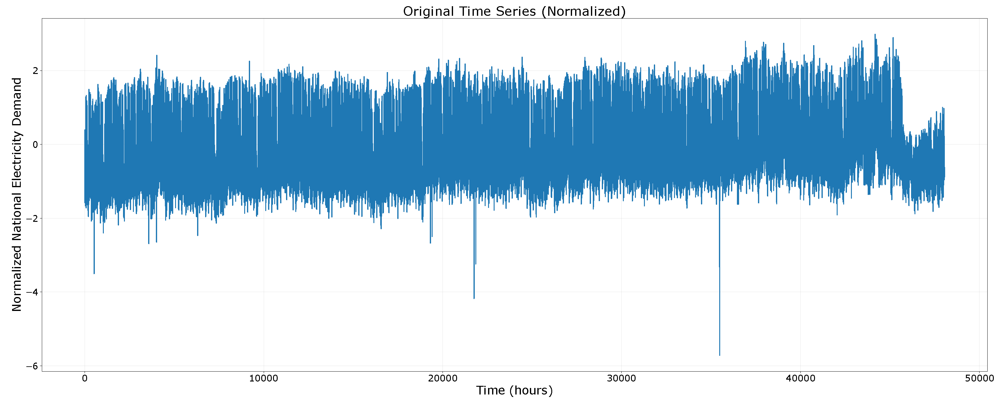
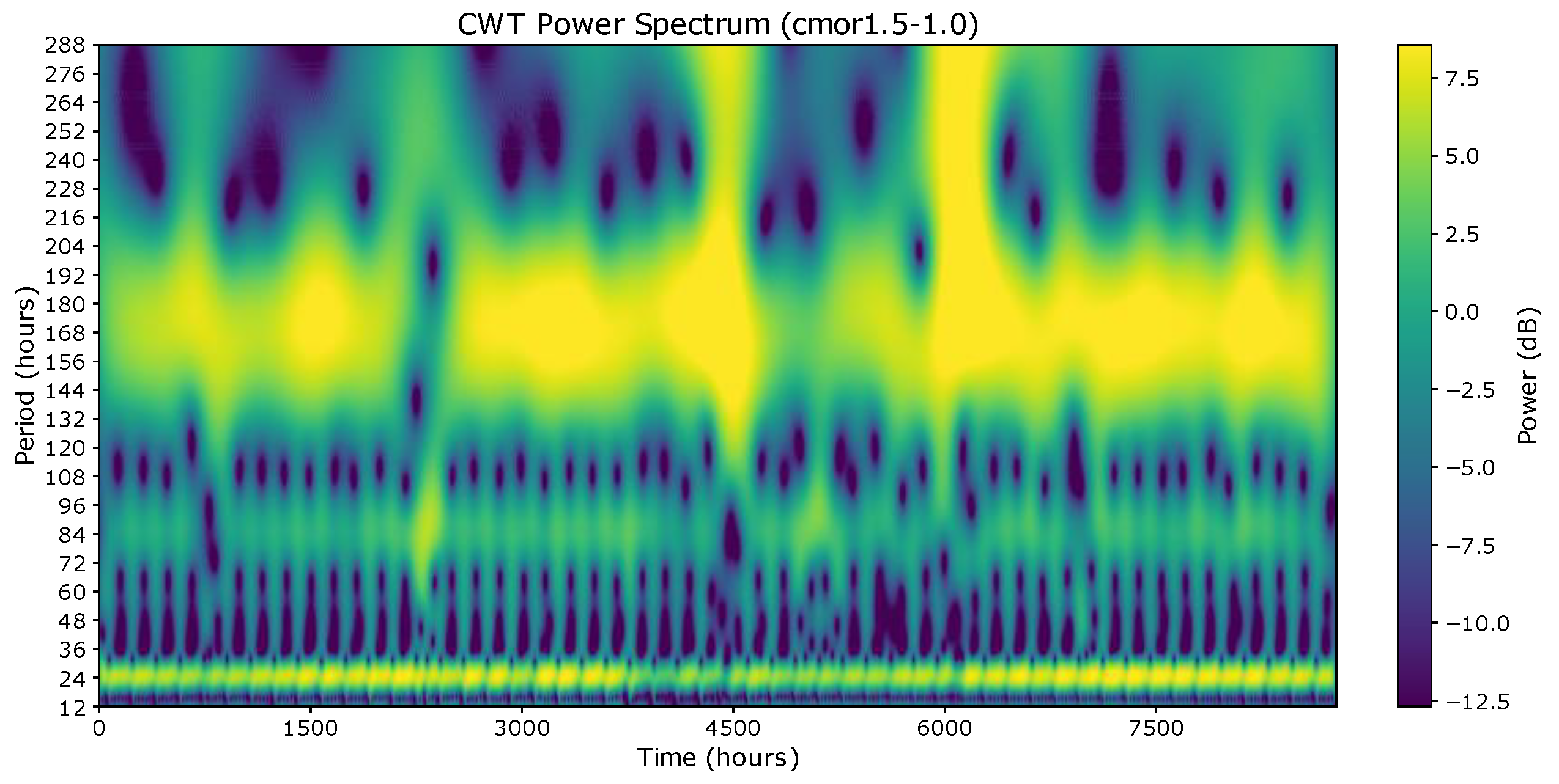
The application of Min-Max normalization was initiated with a dataset that lacked any missing values. The normalized original time series data is displayed in Figure 6. As mentioned in previous sections, attributes other than the national energy demand (nat_demand) attribute are not included in the model estimates due to their low correlation. Conversely, for classical ML and DL methods, lag values in the nat_demand data were incorporated as new attributes. Lags representing these time delay patterns were obtained using CWT analyses. The lag attributes identified through the CWT are subsequently integrated into the RF algorithm within the proposed model, in conjunction with the outcomes derived from the DL model. A primary benefit of calculating these lag values is that they provide an indication of the range within which the DL units in the proposed model will determine long-term patterns. Time lags are capable of capturing conditional dependencies between successive time periods in the model [35]. The process of manually identifying the optimal lag length window is computationally intensive and time-consuming for DL models with many parameters to learn. Consequently, CWT was employed in this study to ascertain the optimal lag length windows. The scales with the highest energy concentrations in the wavelet power spectrum were analyzed to identify dominant periodicities. The CWT analyses, whose time-frequency results are shown in Figure 7, revealed significant patterns (lags) in the 24 h, 84 h, and 168 h time scales. These patterns have been identified as particularly influential in Lag24 and Lag168. These dominant periodicities were then used to define the MSSW lengths. Thus, the selection of 24, 84, and 168 h was not arbitrary but was guided by the most significant periodic components captured through the CWT analysis. Furthermore, a rolling average of national demand values over a week has been incorporated as a feature to mitigate potential noise. This feature serves to mitigate fluctuations in the time series, thereby enhancing the ability to model long-term trends. This mitigates the repercussions of sudden load changes, thereby facilitating a more balanced forecast.

4.2. Model Evaluation

The subsequent experimental stage involves the acquisition of prediction results from classical ML and DL models, in conjunction with the proposed model. The relevant dataset is divided into training and test data at a rate of 80–20% without disrupting their temporal order. The model training was calculated using in-sample training data, and performance was calculated using test data. The forecasting horizon was defined as one hour ahead, employing a direct single-step prediction strategy. To enrich the temporal context, multi-scale sliding windows (MSSW) were incorporated, which feed lagged observations from multiple scales (e.g., 24 h, 84 h, 168 h) into the model as additional input features. The performance of the models was evaluated using the mean absolute error (MAE), root mean squared error (RMSE) and mean absolute percentage error (MAPE) performance metrics. The results were analyzed in a complementary manner by calculating the percentage difference between the actual maximum demand value and the estimated maximum demand value (Peak Error), the percentage difference between the actual minimum demand value and the estimated minimum demand value (Valley Error), and the total energy difference (Energy Error). The mathematical expressions of the metrics utilized are delineated in Equations (5a)–(5f).
M A E = 1 n i = 1 n y i y ^ i
P e a k   E r r o r = max y m a x ( y ^ i ) max y × 100
R M S E = 1 n i = 1 n ( y i y ^ i ) 2
V a l l e y   E r r o r = min y m i n ( y ^ i ) min y × 100
M A P E = 100 n i = 1 n y i y ^ i y i
E n e r g y   E r r o r = i = 1 n y i i = 1 n y ^ i i = 1 n y i × 100  
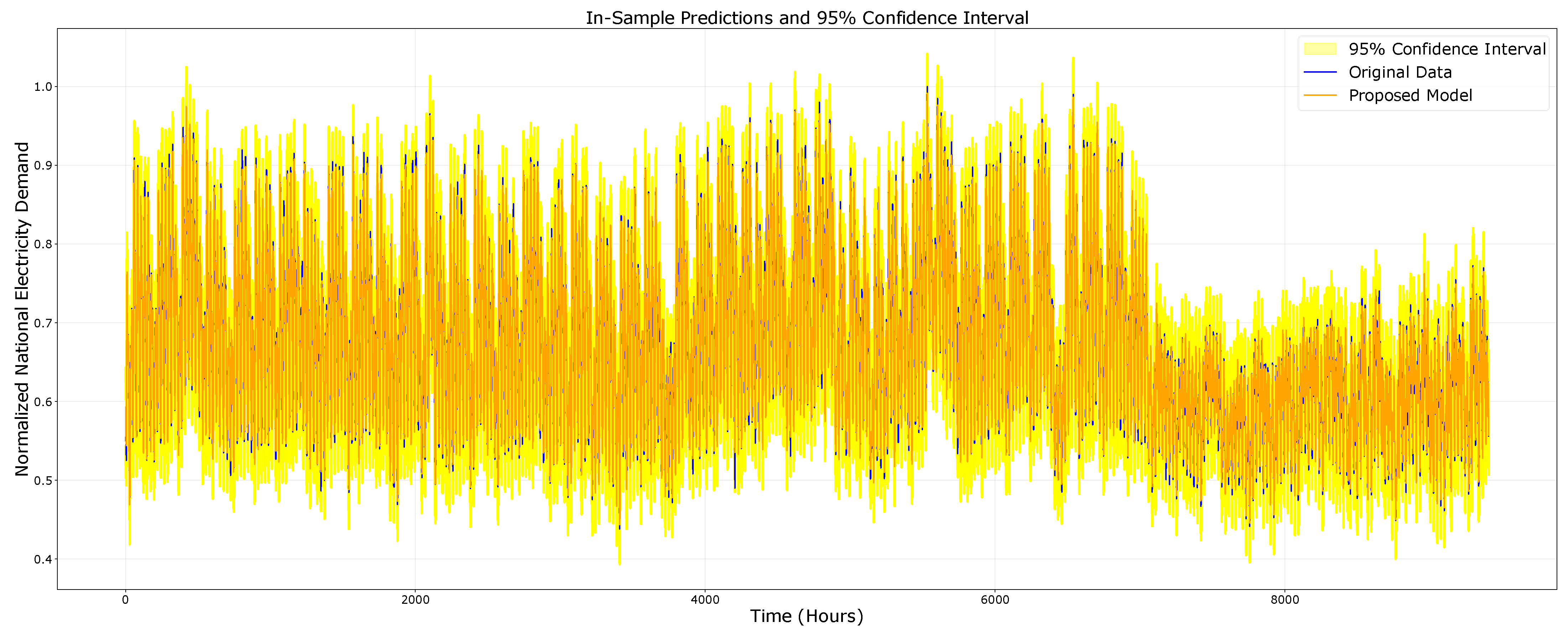
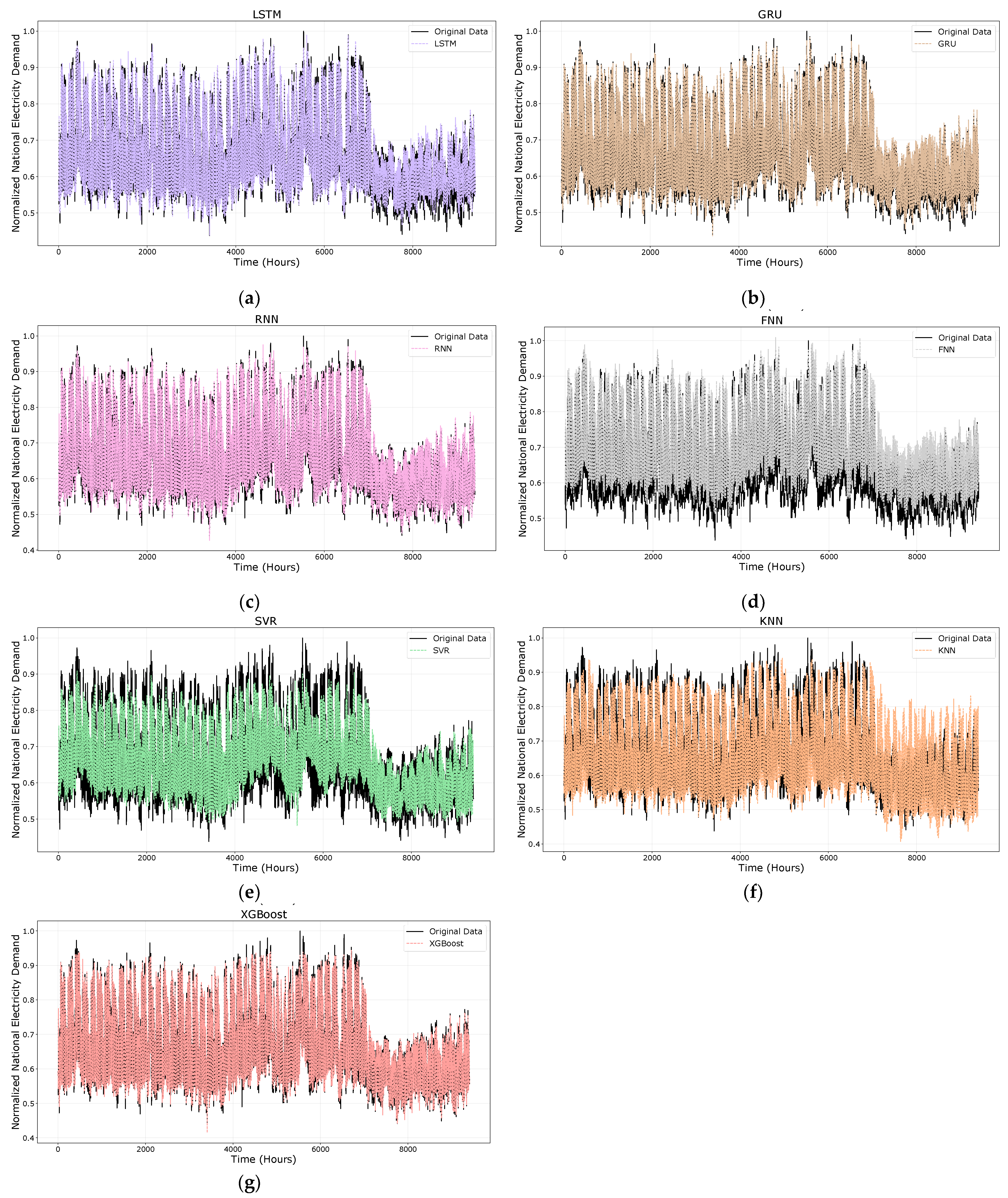
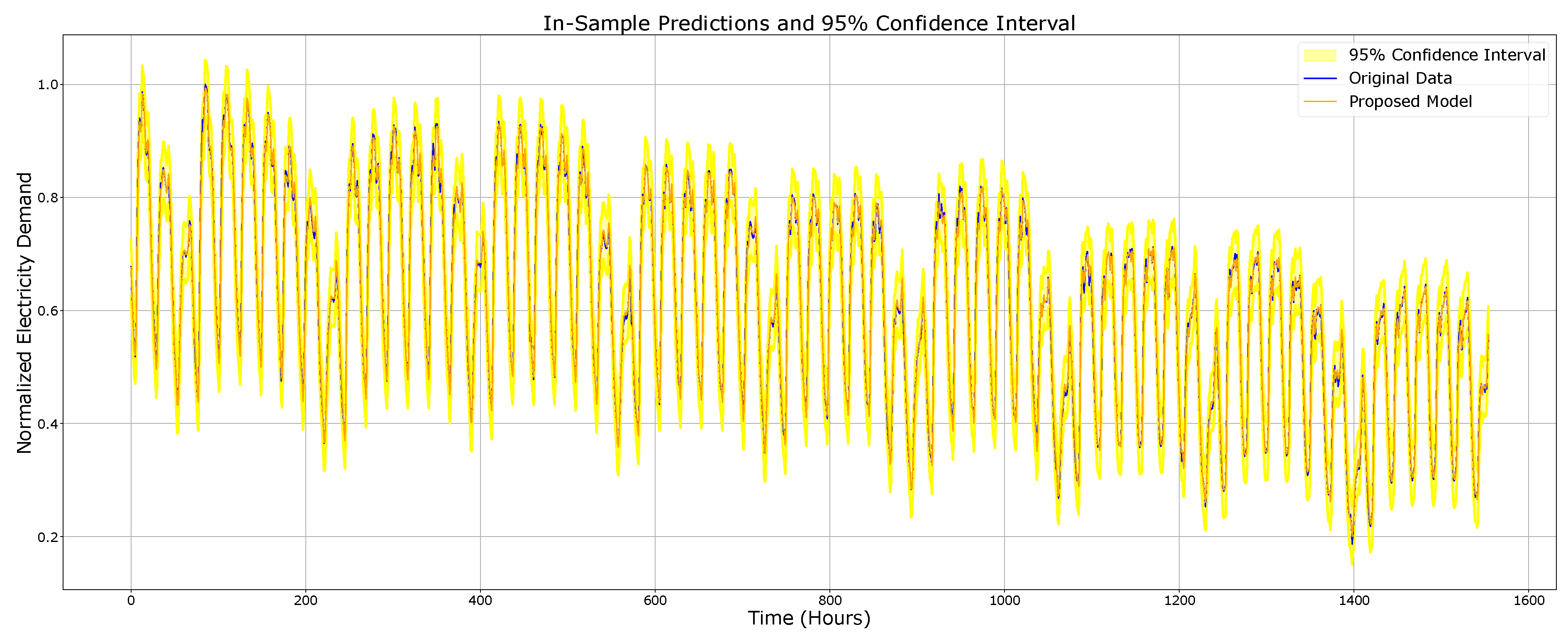
The graphical prediction results of the proposed model are illustrated in Figure 8. The results of the other models are presented in Figure 9a–g. The comparative performance results according to performance metrics are displayed in Table 8. A comparison of the energy demand estimation results of the proposed model with the observed actual energy demand values reveals that the estimations are realized with high accuracy. The model’s efficacy has been demonstrated by its ability to provide a good fit to historical data and to produce stable and reliable predictions, even in situations of uncertainty. These findings indicate that the model possesses a robust forecasting capacity. The stable distribution within the confidence interval suggests that the model is not susceptible to systematic errors, such as overestimation or underestimation, and can effectively capture general energy demand patterns.
Comparative results clearly demonstrate that the proposed model’s predictive performance is superior to that of conventional ML and DL methods based on MAE, RMSE, and MAPE metrics. In a similar vein, the proposed model yielded the most successful results also with the lowest error levels for other complementary error metrics. LSTM has demonstrated a degree of success in capturing general trends and seasonal patterns to a certain extent. However, the LSTM response is often characterized by a delay and a smoothing effect during sudden increases and decreases in demand, suggesting that the model’s capacity to sudden demand changes is constrained. The proposed model exhibits superior representation of sharp transitions and more precise capture of outliers in comparison to the LSTM model. GRU exhibits superiority in capturing peaks and valleys in comparison to LSTM, and responds with greater rapidity to sudden demand changes. However, it is not as proficient as LSTM in following general trends. The GRU prediction curve is smoothed to a greater extent than the proposed model, resulting in a loss of accuracy.
Due to its inherent limitations, the RNN failed to capture both peaks and troughs and often deviated from the mean. This suggests that its simplified structure circumvents overestimation, thereby yielding more stable and generalizable predictions. Due to its absence of a time-dependent structure, FNN demonstrated insensitivity to sudden changes in demand. While the model exhibited some success in capturing peaks during specific time periods, it demonstrated a notable deficiency in accurately capturing troughs. The peak error and valley error values further illustrate this phenomenon. While the model exhibited a moderate degree of representation of the overall trend, it demonstrated substandard forecasting performance, characterized by substantial deviations in certain time periods.
While SVR demonstrates acceptable performance in capturing general trends, it exhibits significant deviations, particularly during periods of sudden increases or decreases in demand. The model’s forecast curve exhibited systematic fluctuations above or below actual values in certain time periods, resulting in an inadequate representation of short-term fluctuations. Notably, substantial deviations were detected, especially during periods of high and low demand, resulting in an expansion of the margin of error. This finding indicates that the SVR for the time series in question may have lacked sufficient sensitivity to complex patterns involving sudden changes, thereby hindering the model’s capacity to effectively learn trends and seasonality over time. This limitation imposed a constraint on the model’s capacity for generalization. The KNN model, which produced analogous predictions based on prior observations, was capable of reflecting these changes with a delay and to a lesser extent during periods when the demand curve exhibited sudden fluctuations. While it was partially successful in the initial 6000 h period, when demand remained relatively stable, it exhibited significant deviations from the prevailing trend. Particularly after 7000 h, when there was a substantial decline in energy demand, significant deviations in the KNN model’s predictions led to a notable increase in error. The KNN predictions exhibited an inability to establish a consistent parallel with the real data, indicating a deficiency in KNN’s capacity to model the seasonal structure of the dataset.
The XGBoost model demonstrated efficacy in capturing the general trend, with its decision trees and incremental learning mechanism. Nevertheless, while the results of the model generally aligned with the actual values, there were instances where the demand forecasts exhibited systematic deviations from the actual demand values. A notable limitation of the model is its inability to accurately predict peaks and troughs. This finding suggests that the model’s capacity to represent extreme values is constrained, indicating that it may have incomplete or inadequately learned seasonal patterns. Nevertheless, the XgBoost model has been demonstrated to exhibit stable and consistent forecasting performance, learning seasonality and trend structure more effectively than the SVR and KNN models.
Conversely, the proposed model yielded the forecast curve closest to the actual data compared to other methods and was able to successfully track both general trends and short-term variations. The model exhibited a forecasting capability that was more sensitive to extreme values, thus producing very fast and realistic forecasts even during periods of sudden demand changes. The efficacy of the model demonstrates the proposed architecture’s substantial capacity to discern dependencies in time series, including trends, seasonality, and sudden fluctuations. This capacity is indicative of the model’s robust generalization abilities. Consequently, the proposed model has been validated to generate more precise and dependable predictions with reduced error rates in comparison to alternative methods. In the context of energy demand forecasting, a field that exerts a direct influence on economic, environmental, and operational decision-making processes, the close proximity of forecasts to actual values suggests the efficacy and reliability of the model in question. This model has the potential to serve as a valuable instrument in various domains, including operational planning, network management, and supply–demand balance.
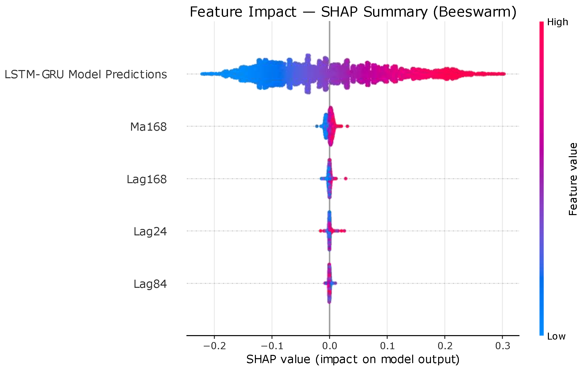
The proposed model’s attributes and their impact on prediction results can be elucidated through analysis of the SHAP summary chart, as presented in Figure 10. The features consist of demand predictions of the primary LSTM-GRU model and Lag24, Lag84, Lag168 and moving average Ma168 features obtained from CWT analyses. The collective impact of these features on the model (as measured by the average absolute SHAP value) can be ascertained by examining their sequence in relation to the graph. This analysis underscores the pronounced impact of the LSTM-GRU Model Predictions feature in comparison to other external features. This feature exerts a predominant influence on the ultimate outcome of the model, as evidenced by its extensive distribution of SHAP values. The Ma168 feature is the second most significant component of the model, functioning as the primary corrective element. The LSTM-GRU Model Predictions feature smooths out the potential errors of the model by correcting the prediction values with a low positive or negative SHAP value in cases where the instantaneous change in demand produces high predictions but the long-term trend is low. Lag168, Lag24, and Lag84 offer minor corrections to model predictions by furnishing supplementary contextual information from particular past time points.
Finally, although it is not one of the primary steps of the experiment, an interim experiment was also conducted to prove how the CWT technique quickly finds the optimum Lag values. In this interim experiment, the performance results of the Lag combinations found in the CWT analyses with the intuitively manually determined Lag values were observed. As illustrated in Table 9, CWT has been demonstrated to effectively identify optimal lag values for all metric values. This finding lends further credence to the computational and temporal advantages of CWT.

4.3. Ablation Studies

To further investigate the contribution of each component in the proposed hybrid framework, an ablation study was conducted. Table 10 presents the results obtained when sequentially removing individual modules, including the LSTM, GRU, CNN-based convolutional filters, and the random forest post-processing stage. The comparison demonstrates the superiority of the full configuration in achieving optimal overall performance, as evidenced by metrics such as MAE, RMSE, and MAPE.
The full model (LSTM + GRU + CNN + RF) exhibited the most optimal performance, achieving the lowest error values across all metrics. The performance of the model underwent a substantial decline when the LSTM branch was removed, thereby underscoring the importance of LSTMs in capturing long-term temporal dependencies. A similar outcome was observed when the GRU was excluded, suggesting that GRUs contribute to the model’s capacity to discern short- and medium-term dynamics. The elimination of the RF stage resulted in a substantial surge in energy-related errors, particularly the valley error and energy error. This finding emphasizes the crucial role of RF in improving forecasts and sustaining aggregate demand consistency. Conversely, the elimination of CNN convolutional filters engendered only a slight performance decline, thereby suggesting that CNNs provide additional local pattern extraction but are less influential compared to recurrent layers.
The results of the ablation study have demonstrated that each component contributes to the predictive accuracy, and that the joint integration of these components in the FULL architecture provides the most accurate and robust forecasts.

4.4. Evaluation of Generalization Performance on a Secondary Dataset

Model flexibility is a crucial component of enhanced system adaptability, ensuring the prediction framework maintains its robustness under changing operational conditions [47]. In this context, additional testing was conducted on a second dataset not utilized in the training process to validate the generalization ability of the proposed model. The dataset under consideration encompasses a variety of consumption profiles, demand patterns, and data distributions. The findings indicate that the model does not overfit to a particular dataset; rather, it produces consistent and reliable predictions under diverse conditions.
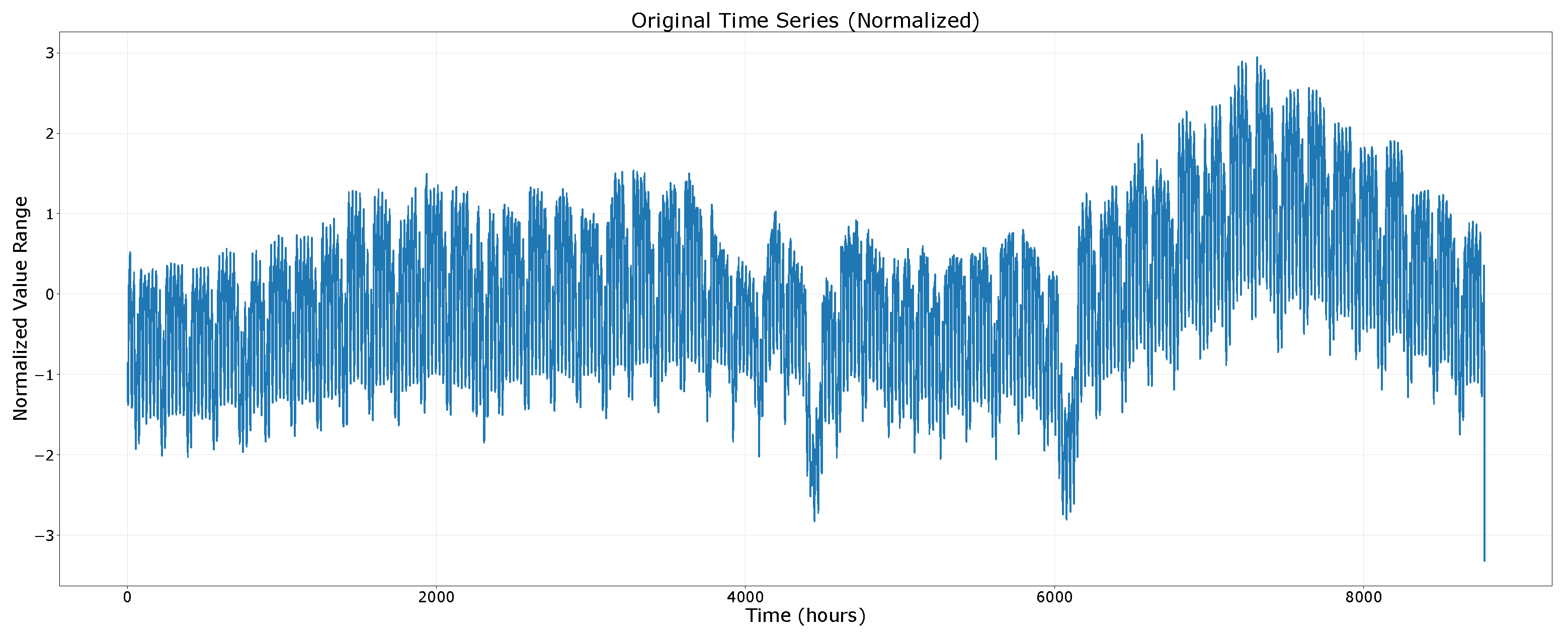
The study utilized a dataset obtained from the EPİAŞ Transparency Platform, which displays real-time consumption in Turkey. This particular dataset is of an annual nature, comprising a total of 8783 hourly data points, encompassing the period from 27 September 2024, to 27 September 2025. The normalized original time series data is displayed in Figure 11, while the CWT analyses are displayed in Figure 12.
CWT analyses of the second dataset once again revealed significant patterns across 24, 84, and 168 h timeframes. A moving average of weekly consumption values was incorporated as a feature of the system. Figure 13 shows the graphical prediction results of the proposed model. Table 11 shows the comparative performance results according to performance metrics.
The forecasting results obtained from the second dataset demonstrate that the proposed model consistently exhibits superior forecasting performance in comparison to other ML and DL methods. In contrast to the other approaches that demonstrated relatively high error rates across most error metrics, the proposed model exhibited significantly higher forecast accuracy, attaining the lowest values for MAE (0.005), RMSE (0.006), and MAPE (0.93%). Furthermore, it achieved substantial reductions in error levels across the peak, valley, and energy error metrics (0.40%, 8.23%, and 0.0032%, respectively), surpassing the performance of other methods. These results confirm that the proposed hybrid model not only effectively generalizes to an independent dataset but also provides more reliable and stable demand forecasts compared to traditional ML and DL methods.

5. Conclusions

In this study, a hybrid model combining LSTM, GRU and random forest models is proposed to improve energy demand forecasting performance. Moreover, the proposed model is supported by the MSSW approach and utilizes CWT analysis to ascertain the optimal window sizes. The findings indicated consistent enhancements over classical ML and DL baselines on the Panama dataset, underscoring the model’s capacity to capture multi-scale temporal dependencies. The MSSW structure’s capacity to discern demand patterns across diverse temporal scales, bolstered by CWT, enables efficient pattern learning and offers a more adaptable solution in comparison to the conventional sliding window approach. Furthermore, CWT has demonstrated remarkable proficiency in the extraction of patterns that elude capture through human experience and perception. The model design is characterized by its emphasis on reproducibility and cross-dataset validation, which contributes to the robustness of forecasting research. Moreover, the proposed model can improve forecasting of critical demand fluctuations, enabling operators to schedule generation units more efficiently, reduce unnecessary reserve activation, and minimize the risk of supply–demand imbalances. This translates into lower forecasting errors and improvements in system reliability and cost efficiency. In summary, the present work contributes to ongoing research in energy demand forecasting by proposing a hybrid framework that leverages multi-scale windowing and CWT analysis to identify the optimal window size.
The study has limitations. The evaluation was based on two datasets, excluding factors like weather, electricity prices, and socio-economic indicators. The forecasting horizon was constrained to hourly predictions, and the model’s applicability to multi-step horizons is under investigation. The hybrid model demonstrates accuracy, but its computational complexity may hinder scalability to very large datasets or real-time operational environments. Although the model was designed for hardware implementation, real-time deployment and integration into operational decision-making processes were not thoroughly evaluated.
Subsequent studies will entail the incorporation of external variables into the model, the execution of hyperparameter optimization, and the assessment of the model’s performance in real-world settings on embedded systems. Exploring lightweight architectures or optimization techniques could enhance scalability and facilitate real-time deployment on embedded devices. Expanding reproducibility practices and integrating the model into operational decision-making processes would strengthen its practical relevance.

Author Contributions

Conceptualization, E.S. and G.Y.; methodology, E.S.; software, E.S. and G.Y.; validation, G.Y. and M.T.Ö.; investigation, E.S.; resources, E.S.; data curation, E.S. and G.Y.; writing—original draft preparation, E.S.; writing—review and editing, G.Y. and M.T.Ö.; visualization, E.S.; supervision, G.Y. and M.T.Ö. All authors have read and agreed to the published version of the manuscript.

Funding

This research received no external funding.

Data Availability Statement

The study utilized a publicly accessible dataset [https://www.kaggle.com/datasets/ernestojaguilar/shortterm-electricity-load-forecasting-panama (accessed on 2 September 2025)] comprising real-time energy demand records for Panama. The raw data supporting the conclusions of this article will be made available by the authors upon request.

Acknowledgments

The present work is grounded in E.S.’s doctoral thesis, which was conducted at the Graduate School of Natural and Applied Sciences, Fırat University, Elazığ, Turkey, within the domain of Electrical and Electronics Engineering at Munzur University.

Conflicts of Interest

The authors declare no conflicts of interest.

Abbreviations

The following abbreviations are used in this manuscript:
CWTContinuous Wavelet Transform
DLDeep Learning
FNNFeedforward Neural Network
GRUGated Recurrent Unit
KNNK-Nearest Neighbors
LSTMLong Short-Term Memory
MLMachine Learning
RNNRecurrent Neural Network
SVRSupport Vector Regression
XGBoostExtreme Gradient Boosting

References

  1. Atputharajah, A.; Saha, T.K. Power System Blackouts—Literature Review. In Proceedings of the 2009 International Conference on Industrial and Information Systems (ICIIS), Peradeniya, Sri Lanka, 28–31 December 2009; pp. 460–465. [Google Scholar]
  2. Wang, Y.; Gu, A.; Zhang, A. Recent Development of Energy Supply and Demand in China, and Energy Sector Prospects through 2030. Energy Policy 2011, 39, 6745–6759. [Google Scholar] [CrossRef]
  3. Zhang, J.; Wang, Y.; Hug, G. Cost-Oriented Load Forecasting. Electric Power Systems Research 2022, 205, 107723. [Google Scholar] [CrossRef]
  4. Wang, S.; Li, C.; Lim, A. Why Are the ARIMA and SARIMA Not Sufficient. arXiv 2021, arXiv:1904.07632. [Google Scholar] [CrossRef]
  5. Aderibigbe, A.O.; Ani, E.C.; Ohenhen, P.E.; Ohalete, N.C.; Daraojimba, D.O. Enhancing Energy Efficiency With Ai: A Review Of Machine Learning Models In Electricity Demand Forecasting. Eng. Sci. Technol. J. 2023, 4, 341–356. [Google Scholar] [CrossRef]
  6. Benti, N.E.; Chaka, M.D.; Semie, A.G. Forecasting Renewable Energy Generation with Machine Learning and Deep Learning: Current Advances and Future Prospects. Sustainability 2023, 15, 7087. [Google Scholar] [CrossRef]
  7. Fan, Y.; Zhang, Y.; Guo, B.; Luo, X.; Peng, Q.; Jin, Z. A Hybrid Sparrow Search Algorithm of the Hyperparameter Optimization in Deep Learning. Mathematics 2022, 10, 3019. [Google Scholar] [CrossRef]
  8. Aguilar Madrid, E.; Antonio, N. Short-Term Electricity Load Forecasting with Machine Learning. Information 2021, 12, 50. [Google Scholar] [CrossRef]
  9. Lin, J.; Ma, J.; Zhu, J.; Cui, Y. Short-Term Load Forecasting Based on LSTM Networks Considering Attention Mechanism. Int. J. Electr. Power Energy Syst. 2022, 137, 107818. [Google Scholar] [CrossRef]
  10. Aouad, M.; Hajj, H.; Shaban, K.; Jabr, R.A.; El-Hajj, W. A CNN-Sequence-to-Sequence Network with Attention for Residential Short-Term Load Forecasting. Electr. Power Syst. Res. 2022, 211, 108152. [Google Scholar] [CrossRef]
  11. Ibrahim, B.; Rabelo, L.; Gutierrez-Franco, E.; Clavijo-Buritica, N. Machine Learning for Short-Term Load Forecasting in Smart Grids. Energies 2022, 15, 8079. [Google Scholar] [CrossRef]
  12. Joy, C.P.; Pillai, G.; Chen, Y.; Mistry, K. Micro-Genetic Algorithm Embedded Multi-Population Differential Evolution Based Neural Network for Short-Term Load Forecasting. In Proceedings of the 2021 56th International Universities Power Engineering Conference: Powering Net Zero Emissions, UPEC 2021—Proceedings, online, 31 August 2021. [Google Scholar]
  13. Sun, L.; Qin, H.; Przystupa, K.; Majka, M.; Kochan, O. Individualized Short-Term Electric Load Forecasting Using Data-Driven Meta-Heuristic Method Based on LSTM Network. Sensors 2022, 22, 7900. [Google Scholar] [CrossRef]
  14. Shohan, M.J.A.; Faruque, M.O.; Foo, S.Y. Forecasting of Electric Load Using a Hybrid LSTM-Neural Prophet Model. Energies 2022, 15, 2158. [Google Scholar] [CrossRef]
  15. Valencia, V.A.N.; Sanchez-Galan, J.E. Use of Attention-Based Neural Networks to Short-Term Load Forecasting in the Republic of Panama. In Proceedings of the Proceedings of the 2022 IEEE 40th Central America and Panama Convention, CONCAPAN 2022, Panama City, Panama, 9–12 November 2022. [Google Scholar]
  16. Abumohsen, M.; Owda, A.Y.; Owda, M. Electrical Load Forecasting Using LSTM, GRU, and RNN Algorithms. Energies 2023, 16, 2283. [Google Scholar] [CrossRef]
  17. Mounir, N.; Ouadi, H.; Jrhilifa, I. Short-Term Electric Load Forecasting Using an EMD-BI-LSTM Approach for Smart Grid Energy Management System. Energy Build. 2023, 288, 113022. [Google Scholar] [CrossRef]
  18. Farsi, B.; Amayri, M.; Bouguila, N.; Eicker, U. On Short-Term Load Forecasting Using Machine Learning Techniques and a Novel Parallel Deep LSTM-CNN Approach. IEEE Access 2021, 9, 31191–31212. [Google Scholar] [CrossRef]
  19. Ullah, K.; Ahsan, M.; Hasanat, S.M.; Haris, M.; Yousaf, H.; Raza, S.F.; Tandon, R.; Abid, S.; Ullah, Z. Short-Term Load Forecasting: A Comprehensive Review and Simulation Study with CNN-LSTM Hybrids Approach. IEEE Access 2024, 12, 111858–111881. [Google Scholar] [CrossRef]
  20. Ijaz, K.; Hussain, Z.; Ahmad, J.; Ali, S.F.; Adnan, M.; Khosa, I. A Novel Temporal Feature Selection Based LSTM Model for Electrical Short-Term Load Forecasting. IEEE Access 2022, 10, 82596–82613. [Google Scholar] [CrossRef]
  21. Rafi, S.H.; Al-Masood, N.; Deeba, S.R.; Hossain, E. A Short-Term Load Forecasting Method Using Integrated CNN and LSTM Network. IEEE Access 2021, 9, 32436–32448. [Google Scholar] [CrossRef]
  22. Chen, Z.; Jin, T.; Zheng, X.; Liu, Y.; Zhuang, Z.; Mohamed, M.A. An Innovative Method-Based CEEMDAN–IGWO–GRU Hybrid Algorithm for Short-Term Load Forecasting. Electr. Eng. 2022, 104, 3137–3156. [Google Scholar] [CrossRef]
  23. Su, Z.; Zheng, G.; Wang, G.; Hu, M.; Kong, L. An IDBO-Optimized CNN-BiLSTM Model for Load Forecasting in Regional Integrated Energy Systems. Comput. Electr. Eng. 2025, 123, 110013. [Google Scholar] [CrossRef]
  24. Shah, S.A.H.; Ahmed, U.; Bilal, M.; Khan, A.R.; Razzaq, S.; Aziz, I.; Mahmood, A. Improved Electric Load Forecasting Using Quantile Long Short-Term Memory Network with Dual Attention Mechanism. Energy Rep. 2025, 13, 2343–2353. [Google Scholar] [CrossRef]
  25. Asghar Majeed, M.; Phichaisawat, S.; Asghar, F.; Hussan, U. Data-Driven Optimized Load Forecasting: An LSTM-Based RNN Approach for Smart Grids. IEEE Access 2025, 13, 99018–99031. [Google Scholar] [CrossRef]
  26. Zheng, D.; Qin, J.; Liu, Z.; Zhang, Q.; Duan, J.; Zhou, Y. BWO–ICEEMDAN–ITransformer: A Short-Term Load Forecasting Model for Power Systems with Parameter Optimization. Algorithms 2025, 18, 243. [Google Scholar] [CrossRef]
  27. Ahranjani, Y.K.; Beiraghi, M.; Ghanizadeh, R. Short Time Load Forecasting for Urmia City Using the Novel CNN-LTSM Deep Learning Structure. Electr. Eng. 2025, 107, 1253–1264. [Google Scholar] [CrossRef]
  28. Fan, C.; Li, G.; Xiao, L.; Yi, L.; Nie, S. Short-Term Power Load Forecasting in City Based on ISSA-BiTCN-LSTM. Cogn. Comput. 2025, 17, 39. [Google Scholar] [CrossRef]
  29. Feng, Y.; Zhu, J.; Qiu, P.; Zhang, X.; Shuai, C. Short-Term Power Load Forecasting Based on TCN-BiLSTM-Attention and Multi-Feature Fusion. Arab. J. Sci. Eng. 2025, 50, 5475–5486. [Google Scholar] [CrossRef]
  30. Martirosyan, A.; Ilyushin, Y.; Afanaseva, O.; Kukharova, T.; Asadulagi, M.; Khloponina, V. Development of an Oil Field’s Conceptual Model. Int. J. Eng. 2025, 38, 381–388. [Google Scholar] [CrossRef]
  31. Sadowsky, J. Investigation of Signal Characteristics Using the Continuous Wavelet Transform. Johns Hopkins Apl Tech. Dig. 1996, 17, 258–269. [Google Scholar]
  32. Küçük, M.; Ağiralioğlu, N. Dalgacık Dönüşüm Tekniği Kullanılarak Hidrolojik Akım Serilerinin Modellenmesi. İtüdergisi/D 2011, 5, 69–80. [Google Scholar]
  33. Arı, N.; Özen, Ş.; Çolak, Ö.H. Dalgacık Teorisi; Palme Yayıncılık: Ankara, Turkey, 2008; pp. 23–27. [Google Scholar]
  34. Wang, J.; Jiang, W.; Li, Z.; Lu, Y. A New Multi-Scale Sliding Window LSTM Framework (MSSW-LSTM): A Case Study for GNSS Time-Series Prediction. Remote Sens. 2021, 13, 3328. [Google Scholar] [CrossRef]
  35. Bouktif, S.; Fiaz, A.; Ouni, A.; Serhani, M. Optimal Deep Learning LSTM Model for Electric Load Forecasting Using Feature Selection and Genetic Algorithm: Comparison with Machine Learning Approaches. Energies 2018, 11, 1636. [Google Scholar] [CrossRef]
  36. Bouktif, S.; Fiaz, A.; Ouni, A.; Serhani, M.A. Multi-Sequence LSTM-RNN Deep Learning and Metaheuristics for Electric Load Forecasting. Energies 2020, 13, 391. [Google Scholar] [CrossRef]
  37. Kong, W.; Dong, Z.Y.; Jia, Y.; Hill, D.J.; Xu, Y.; Zhang, Y. Short-Term Residential Load Forecasting Based on LSTM Recurrent Neural Network. IEEE Trans. Smart Grid 2019, 10, 841–851. [Google Scholar] [CrossRef]
  38. Son, N.; Shin, Y. Short- and Medium-Term Electricity Consumption Forecasting Using Prophet and GRU. Sustainability 2023, 15, 15860. [Google Scholar] [CrossRef]
  39. Li, W.; Logenthiran, T.; Woo, W.L. Multi-GRU Prediction System for Electricity Generation’s Planning and Operation. IET Gener. Transm. Distrib. 2019, 13, 1630–1637. [Google Scholar] [CrossRef]
  40. Sajjad, M.; Khan, Z.A.; Ullah, A.; Hussain, T.; Ullah, W.; Lee, M.Y.; Baik, S.W. A Novel CNN-GRU-Based Hybrid Approach for Short-Term Residential Load Forecasting. IEEE Access 2020, 8, 143759–143768. [Google Scholar] [CrossRef]
  41. Gao, X.; Li, X.; Zhao, B.; Ji, W.; Jing, X.; He, Y. Short-Term Electricity Load Forecasting Model Based on EMD-GRU with Feature Selection. Energies 2019, 12, 1140. [Google Scholar] [CrossRef]
  42. Ke, K.; Hongbin, S.; Chengkang, Z.; Brown, C. Short-Term Electrical Load Forecasting Method Based on Stacked Auto-Encoding and GRU Neural Network. Evol. Intell. 2019, 12, 385–394. [Google Scholar] [CrossRef]
  43. Dudek, G. A Comprehensive Study of Random Forest for Short-Term Load Forecasting. Energies 2022, 15, 7547. [Google Scholar] [CrossRef]
  44. Chen, Y.-T.; Piedad, E.; Kuo, C.-C. Energy Consumption Load Forecasting Using a Level-Based Random Forest Classifier. Symmetry 2019, 11, 956. [Google Scholar] [CrossRef]
  45. Li, C.; Tao, Y.; Ao, W.; Yang, S.; Bai, Y. Improving Forecasting Accuracy of Daily Enterprise Electricity Consumption Using a Random Forest Based on Ensemble Empirical Mode Decomposition. Energy 2018, 165, 1220–1227. [Google Scholar] [CrossRef]
  46. Mallala, B.; Ahmed, A.I.U.; Pamidi, S.V.; Faruque, M.O.; Reddy M, R. Forecasting Global Sustainable Energy from Renewable Sources Using Random Forest Algorithm. Results Eng. 2025, 25, 103789. [Google Scholar] [CrossRef]
  47. Sui, Q.; He, H.; Liang, J.; Li, Z.; Su, C. Short-Term Scheduling of Integrated Electric-Hydrogen-Thermal Systems Considering Hydroelectric Power Plant Peaking for Hydrogen Vessel Navigation. IEEE Trans. Sustain. Energy 2025, 16, 3082–3094. [Google Scholar] [CrossRef]
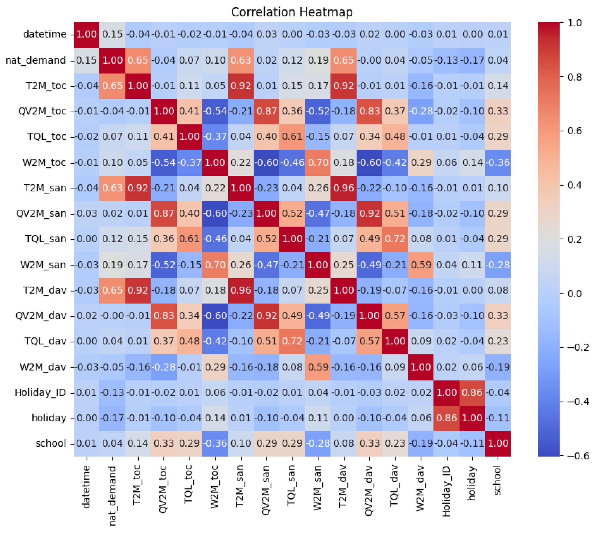
Figure 1. Correlation heatmap of the dataset.
Applsci 15 10801 g001
Figure 2. Energy demand characteristics for monthly, daily, hourly and holidays. (a) Monthly Data Distribution; (b) Daily Data Distribution; (c) Hourly Data Distribution; (d) Weekend/Holiday Data Distribution.
Applsci 15 10801 g002
Figure 3. Architecture of the proposed AI model for demand prediction.
Applsci 15 10801 g003
Figure 4. General architecture of an LSTM.
Applsci 15 10801 g004
Figure 5. General architecture of a GRU.
Applsci 15 10801 g005
Figure 6. Normalized original time series.
Applsci 15 10801 g006
Figure 7. CWT Power spectrum of the dataset.
Applsci 15 10801 g007
Figure 8. In-sample national energy demand forecast curve of the proposed model.
Applsci 15 10801 g008
Figure 9. In-sample national energy demand forecast curves of other models. (a) LSTM model; (b) GRU model; (c) RNN model; (d) FNN model; (e) SVR model; (f) KNN model; (g) XGBoost model.
Applsci 15 10801 g009
Figure 10. Random Forest SHAP summary plot.
Applsci 15 10801 g010
Figure 11. Normalized original time series for EPİAŞ dataset.
Applsci 15 10801 g011
Figure 12. CWT Power spectrum for EPİAŞ dataset.
Applsci 15 10801 g012
Figure 13. In-sample energy demand forecast curve of the proposed model (EPİAŞ dataset).
Applsci 15 10801 g013
Table 1. Detailed comparative summary of recent works.
Work/SourceDatasetInput FeaturesMethod/ModelKey Results of the Error Metrics
IDBO-optimized CNN-BiLSTM [23]Arizona State University (RIES) load operation data (Electrical (EL), Cooling (CL), Heat (HL)). One full year (8760 data points).Multi-energy loads (EL, CL, HL). Min-Max scaling applied.CNN-BiLSTM model optimized using the Improved Dung-Beetle Optimization (IDBO) algorithm to tune hyperparameters. CNN extracts features; BiLSTM learns time series dependencies.EL: MAPE: 3.46%, RMSE: 956.45, R2: 0.98. CL: MAPE: 3.02%, RMSE: 178.21, R2: 0.98. HL: MAPE: 1.97%, RMSE: 17.25, R2: 0.98.
DA-QLSTM [24]IESCO (Islamabad Electric Supply Company, 13,128 points, 2 years) and Panama City (48,048 points, 6 years) load data.IESCO: Temperature, dew point, humidity. Panama: Temperature, relative humidity, wind speed. MinMax scaled.DA-QLSTM (Quantile LSTM with Dual Attention Mechanism). Integrates temporal and feature-wise attention. Uses a custom quantile loss function for probabilistic forecasts (predicting 0.5, 0.6, 0.9 quantiles).IESCO: MAPE: 4.06%, RMSE: 64.62, MAE: 41.61. Panama: MAPE: 1.66%, RMSE: 27.83, MAE: 19.17.
RNN-LSTM [25]Historical load, renewable energy generation, and weather data (Smart Grids/Power Systems).Historical load values and external features (weather, time).RNN-LSTM (Recurrent Neural Network with LSTM units). Optimizes MSE loss using Adam optimizer.RMSE: 2.2889, MAE: 1.104, MAPE: 1.538%
BWO–ICEEMDAN–iTransformer [26]Singapore electricity load, price, and weather data (2019–2020), 30 min intervals.Decomposed load subsequences. Highly correlated factors selected via SCC: Electricity Price, Relative Humidity, and Temperature. Input sequence length 96, output 48.BWO–ICEEMDAN–iTransformer. ICEEMDAN decomposes data. BWO (Beluga Whale Optimization) optimizes ICEEMDAN parameters (Nstd, NR). iTransformer predicts decomposed components.R2: 0.9873, MAE: 48.0014, RMSE: 66.2221.
CNN-LSTM [27]Urmia City (Iran) load and weather data, 3 consecutive years (2009–2011).Historical load consumption trends and upcoming weather conditions.Hybrid CNN-LSTM Deep Learning Structure. CNN extracts features; 3-layer LSTM performs time series prediction. Includes a Dropout layer to mitigate overfitting.MAPE: 0.956%, RMSE: 1.476.
ISSA-BiTCN-LSTM [28]Electric load and weather data from Los Angeles, Tetouan, and Johor.Power load and weather features (Temperature, Humidity, Wind speed, etc.), varying by city.ISSA-BiTCN-LSTM. Parallel hybrid model combining BiTCN (local features) and LSTM (long-term dependencies). ISSA (Improved Salp Swarm Algorithm) optimizes 5 hyperparameters (kernel size, filters, batch size, epochs, neurons).RMSE: 925.11 kW, MAE: 732.63 kW, NRMSE: 0.019, MAPE: 1.034%.
TCN-BiLSTM-Attention [29]Australia regional load, electricity price, and meteorological data (2006–2010), 30 min intervals.Multivariate Time Series: Power Load, Electricity Price, Dry Bulb Temperature, Dew Point Temperature, Wet Bulb Temperature, Humidity.TCN-BiLSTM-Attention. Hybrid architecture: TCN (temporal feature extraction) + BiLSTM (long/short-term dependencies) + Attention Mechanism (multivariate correlation and weighting). Optimized using Grid Search.MAE: 225.531, RMSE: 276.792, MAPE: 2.8%, R2: 0.959
Table 2. Description of dataset characteristics.
Column NameDescriptionUnit
datetimeDate-time index corresponding to Panama time-zone UTC-05:00 (index)
nat_demandNational electricity load (Target or Dependent variable)MWh
T2M_tocTemperature at 2 m in Tocumen, Panama City°C
QV2M_tocRelative humidity at 2 m in Tocumen, Panama City%
TQL_tocLiquid precipitation in Tocumen, Panama City L / m 2
W2M_tocWind Speed at 2 m in Tocumen, Panama Citym/s
T2M_sanTemperature at 2 m in Santiago city°C
QV2M_sanRelative humidity at 2 m in Santiago city%
TQL_sanLiquid precipitation in Santiago city L / m 2
W2M_sanWind Speed at 2 m in Santiago citym/s
T2M_davTemperature at 2 m in David city°C
QV2M_davRelative humidity at 2 m in David city%
TQL_davLiquid precipitation in David city L / m 2
W2M_davWind Speed at 2 m in David citym/s
Holiday_IDUnique identification numberinteger
HolidayHoliday binary indicator1 = holiday, 0 = regular day
schoolSchool period binary indicator1 = school, 0 = vacations
Table 3. Explanations of CWT parameters.
ParameterExplanation
sScale parameter
(s > 1: the function expands over time axis and the amplitude decreases)
(s < 1: the function shrinks over time axis and the amplitude grows)
(s < 0: the symmetry is defined in relation to the point t = 0)
τ Shift parameter
(τ > 0: a shift to the right in the time axis)
(τ < 0: a shift to the left in the time axis)
1 s Normalization factor with different scales
x t Function to be transformed
ψ s , τ * t τ s Complex conjugate of the wavelet function
Table 4. Characteristics of the components of the proposed AI model for demand prediction.
LayerLayer NameOther Layer ParametersOutput ShapeParams
1Input Layer-(168, 5)0
2LSTMactivation = tanh, return_sequences = True(168, 64)17,920
3Conv1Dactivation = linear, padding = causal, strides = (1,)(168, 64)704
4Conv1Dactivation = linear, padding = causal, strides = (1,)(168, 64)704
5Conv1Dactivation = linear, padding = causal, strides = (1,)(168, 64)704
6Concatenate-(168, 256)0
7GRUactivation = tanh, return_sequences = True(168, 64)61,824
8Flatten-(10,752, 1)0
9Denseactivation = relu(32, 1)344,096
10Denseactivation = linear(1, 1)33
Total params: 1,277,957
Trainable params: 425,985
Non-trainable params: 0
Optimizer params: 851,972
Optimizer: Adam
Loss function: MSE
Learning rate: 0.001
Batch size: 32
Epoch: 50
Table 5. Parameters of mathematical models of LSTM.
ParameterExplanation
f t ,   i t ,   o t Forget gate output, input gate output, output gate output
σ Sigmoid activation function
W f ,   W i ,   W o ,   W C Forget gate weight matrix, input gate weight matrix, output gate weight matrix, cell weight matrix
h t 1 Previous hidden state
x t Input at time t
b f ,   b i ,   b o ,   b C Bias vectors
C ~ t Candidate cell state
C t ,   C t 1 Current cell state, previous cell state
h t Current hidden state (Its output is transferred to the next time step and the model.)
Table 6. Parameters of mathematical models of GRU.
ParameterExplanation
z t ,   r t Update gate vector, reset gate vector
σ Sigmoid activation function
W z ,   W r ,   W h Update gate weight matrix, reset gate weight matrix, weight matrix for input data
h t 1 Previous hidden state
x t Input at time t
b z ,   b r ,   b h Bias vectors
h ~ t Candidate hidden state
U z ,   U r ,   U h Weight matrices for recurrent connections
h t Current hidden state
Table 7. Parameters of mathematical models of Random Forest.
ParameterExplanation
f t ( x ) Prediction   of   the   t - th   decision   tree   for   input   x
l t ( x ) Number of samples in that leaf node
i l t ( x ) y i The sum of the target values of all training samples in the corresponding leaf node
y ^ Final   prediction   of   the   Random   Forest   for   input   x
T Total number of decision trees in the forest
Table 8. Comparative results of the proposed model.
MethodMAERMSEMAPE (%)Peak Error (%)Valley Error (%)Energy Error (%)
LSTM0.0170.0222.5491.0690.3140.0306
GRU0.0160.0212.4681.7350.6150.7425
RNN0.0140.0192.1522.5092.4930.4935
FNN0.0410.0486.4471.01611.2505.8283
SVR0.0350.0445.1569.09710.1080.7697
KNN0.0400.0576.1255.9056.9320.2542
XGBoost0.0130.0181.9855.5235.4010.0622
Proposed Model0.0070.0091.0510.8461.2330.0015
Table 9. In-sample performance results for various lag values.
Lag ValuesMAERMSEMAPE (%)Peak Error (%)Valley Error (%)Energy Error (%)
24, 84, 168, ma1680.0070.0091.0510.8461.2330.0015
24, 48, ma1680.0150.0202.2810.9042.9390.0098
24, 72, ma1680.0080.0101.0750.4361.4570.0005
24, 96, ma1680.0280.0384.2874.5637.1600.0173
24, 168, ma1680.0070.0091.1200.5631.5470.0033
24, 48, 72, ma1680.0270.0364.1113.2397.9740.0024
24, 48, 96, ma1680.0070.0101.1760.4171.7950.0004
24, 48, 168, ma1680.0220.0293.4012.8413.2630.0017
24, 72, 168, ma1680.0070.0101.1290.5561.2020.0038
24, 96, 168, ma1680.0150.0202.2651.5981.8800.0067
24, 48, 72, 96, ma1680.0110.0141.6310.7482.3250.0011
24, 48, 72, 168, ma1680.0080.0101.1880.6891.3230.0001
Table 10. Ablation study results of the proposed hybrid model. The FULL model achieves the lowest MAE, RMSE, and Energy Error compared to its ablated versions, demonstrating the contribution of each component.
ConditionMAERMSEMAPE (%)Peak Error (%)Valley Error (%)Energy Error (%)
-Random Forest0.0100.0131.4781.4223.9370.2169
-LSTM0.0250.0333.6703.1722.7370.0133
-GRU0.0140.0182.1081.0211.6050.0060
-CNN0.0080.0101.1300.8691.4870.0017
FULL Model0.0070.0091.0510.8461.2330.0015
Table 11. Comparative results of the proposed model (EPİAŞ dataset).
MethodMAERMSEMAPE (%)Peak Error (%)Valley Error (%)Energy Error (%)
LSTM0.0440.0538.4450.01826.3266.3093
GRU0.0260.0364.4050.80924.4222.1734
RNN0.0380.0497.0052.4181.6582.7249
FNN0.0450.0517.5666.95915.7716.9249
SVR0.0920.12414.53721.07126.3796.6130
KNN0.0530.0699.06111.81835.2661.1835
XGBoost0.0270.0364.40414.2225.5190.7836
Proposed Model0.0050.0060.9250.3998.2270.0032
Disclaimer/Publisher’s Note: The statements, opinions and data contained in all publications are solely those of the individual author(s) and contributor(s) and not of MDPI and/or the editor(s). MDPI and/or the editor(s) disclaim responsibility for any injury to people or property resulting from any ideas, methods, instructions or products referred to in the content.