Abstract
In the process of large-scale water conservancy and hydropower station construction in the southwest region of China, obtaining the deep overburden pressuremeter modulus Em is of great significance for the calculation of foundation bearing capacity and dam foundation settlement. However, due to the complex nature of the soil properties in deep overburden layers, conducting deep-hole pressuremeter tests is challenging, time-consuming, and costly. In order to efficiently and accurately obtain the pressuremeter modulus of deep overburden, this paper takes the deep overburden in the river valley where a large hydropower station dam is located in the southwest region as the research object. It proposes a method based on data-driven prediction of the pressuremeter modulus and combines it with the physical mechanism to carry out the reliability analysis of the prediction results. By constructing a database of soil physical and mechanical parameters, including the pressuremeter modulus, the prediction performance of Random Forest (RF), Support Vector Regression (SVR), and BP Neural Network on the pressure modulus was evaluated. The Particle Swarm Optimization (PSO) was utilized for hyperparameter optimization to enhance the reliability of prediction results. The results indicate that the RF and PSO-RF models exhibit a comprehensive advantage for accurately predicting the pressuremeter modulus. The prediction results of the model for new data have a strong correlation with the results calculated by the Menard formula, which demonstrates the reliability of the model. Therefore, establishing the relationship between the conventional physical and mechanical parameters of deep overburden and the pressuremeter modulus, and predicting the pressuremeter modulus based on data-driven methods, has significant engineering value for obtaining the pressuremeter modulus of deep overburden efficiently, economically, and reliably. It also holds significant importance for the extended application of machine learning in the field of soil parameter prediction.
1. Introduction
Overburden is a general term for loose accumulations and sediments that cover the bedrock due to various geological processes [1]. Meanwhile, a deep overburden in the riverbed refers to Quaternary loose accumulations in the riverbed with a thickness greater than 30 m. Deep and thick overburden layers are widely distributed in various countries and regions around the world. In many parts of the world, numerous major water conservancy projects have been built on deep overburden, such as the famous Aswan Dam, Manic Dam, and Serre Poncon Dam. The characteristics of the deep overburden in Europe and America are dominated by glacial facies, with relatively uniform material composition, continuous stratification, a relatively single sedimentary environment, and good horizontal and vertical continuity. In contrast, the southwest region of China is located at the eastern part of the Qinghai–Tibet Plateau, with a complex geological environment and strong neotectonic movement. Its deep overburden is dominated by fluvial facies, and its genesis is relatively complex. Overall, it presents characteristics of deep thickness, multiple layers, loose structure, and uneven compactness. The lithology in this region varies significantly in both horizontal and vertical directions. With the continuous development of large-scale hydropower projects in Southwest China, the lack of research on the properties of deep overburden soils has led to increasingly prominent construction risks and geological disasters. Among them, issues related to the safety of high earth-rock dams built on deep overburden foundations [2], the design of dam foundations bearing capacity, and the analysis of dam seepage stability [3] are all closely related to the accurate acquisition of foundation parameters. Due to the significant heterogeneity and complex historical genesis of deep overburden in the southwest region, in situ field tests are of greater engineering value in determining the initial physical and mechanical properties of the soil compared to laboratory experiments [4]. In the in situ test of deep overburden, the pressuremeter test is one of the most widely used geotechnical engineering investigation methods. Its working principle is to set up a side pressure instrument at the test depth and transmit the pressure to the surrounding soil through the expansion of the pressuremeter membrane, causing the soil to fail and obtaining the relationship between the radial stress and strain of the soil around the hole [5,6]. From the pressuremeter test, important geotechnical parameters such as the pressuremeter modulus Em, the plastic critical pressure Pf, and the ultimate pressure Pl can be obtained. Among them, the pressuremeter modulus is of great value for the evaluation of soil bearing capacity and the calculation of settlement [7]. Therefore, accurately obtaining the pressuremeter modulus of soil bodies is of significant importance for engineering construction on deep overburden layers and disaster prevention and mitigation.
The pressuremeter test is a time-consuming and costly in situ field test. In order to reduce its operational difficulty, improve test efficiency, and economic benefits, many scholars have conducted extensive research to accurately obtain the relationship between the pressuremeter modulus and other geotechnical parameters. Menard [8] proposed that the pressuremeter modulus is related to the soil elastic modulus as Em = αE0, where α is the structural coefficient of the soil body, and its value is between 0 and 1. Goh et al. [9] suggested that the pressuremeter modulus has a certain correlation to the SPT-N value. Biarez et al. [10] derived the pressuremeter modulus from the numerical simulation of the pressuremeter test. Fawaz et al. [11] obtained the ratio relationship between the pressuremeter modulus and the elastic modulus through the combination of the pressuremeter test and numerical simulations. The existing research methods mainly consider the nonlinear stress–strain relationship of soil, the elastoplastic theory of soil under loading and unloading conditions, and the influence of stress history, and they are derived or fitted with a limited number of linear or nonlinear formulas. However, these methods cannot take into account the high nonlinear relationship between the pressuremeter modulus and the physical properties and mechanical parameters of the soil. Therefore, more scientific and advanced methods are needed to establish the connection between these soil parameters.
In recent years, with the rapid development of computer technology, Computational Intelligence (CI) technology has been increasingly applied in various fields. The principle is to establish appropriate prediction models through learning from a large amount of data. Among them, technologies such as artificial intelligence and machine learning have been utilized in various fields of geotechnical engineering, including slope stability analysis [12,13,14], settlement prediction analysis [15,16,17,18], and tunnel excavation domain [19,20,21]. In addition, many scholars have conducted research on geotechnical parameters, establishing the relationship between input soil parameters and predicted parameters through data-driven methods. For example, Bardhan et al. [22], Mohammadzadeh et al. [23], Kalantary et al. [24], and Nguyen et al. [25] conducted research on the prediction of soil compression index through machine learning models or neural network models; Ehsan et al. [26] established the relationship between pore water pressure in the well and rock physical and mechanical parameters by GBR algorithm; Ziaie Moayed et al. [27] established the relationship between moisture content, plasticity index, and SPT standard penetration number with the pressuremeter modulus through the GMDH neural network model and realized the prediction of the pressuremeter modulus; Moayedi et al. [28] mixed four types of neural network models to achieve the prediction of soil shear strength; Tizpa et al. [29] and Khatti et al. [30] established a connection between soil fine particle content, liquid limit, plastic limit, specific gravity, and other indicators with the maximum dry density of soil through neural networks, and achieved accurate prediction; and Feng et al. [31] achieved the prediction of the elastic modulus of cement soil by the improved convolutional long short-term memory model. In recent years, most scholars have primarily focused on the conventional mechanical parameters of soil (such as compression modulus, compression coefficient, and elastic modulus) or the prediction and analysis of pressuremeter modulus under conventional stratum conditions. However, compared to these parameters, the research on the in situ prediction of pressuremeter modulus in deep overburden layers is still insufficient, and there are fewer studies on the reliability analysis of prediction results based on physical mechanisms. Due to the complexity of the properties of deep overburden soil layers and their relatively thick depth, conducting traditional pressuremeter tests to obtain the pressuremeter modulus is more difficult and challenging compared to conventional environments. Therefore, predicting the pressuremeter modulus through data-driven methods is an effective approach.
Based on this, this paper takes the deep overburden of a hydropower project in the southwest region of China as the research object. By collecting the physical and mechanical parameters of the deep overburden in the riverbed at the dam site area, the Random Forest model (RF) [32,33,34], Support Vector Machine model (SVM) [35,36,37], and BP Neural Network model [38,39,40] are employed, respectively. A relationship between the conventional physical and mechanical indicators of the soil layer and the pressuremeter modulus is established to achieve the prediction of the pressuremeter modulus. Based on this, the prediction of the model is optimized and improved through the Particle Swarm Optimization algorithm (PSO) [41,42,43]. The optimal model for predicting the pressuremeter modulus is determined through comparative analysis. Finally, the reliability of the prediction results is verified based on the physical mechanism analysis of the pressuremeter modulus, thereby ensuring the validity of the model and providing a new approach for obtaining the parameters of the pressuremeter modulus. The research methodology is also significant for the development of machine learning in the field of geotechnical in situ test parameter prediction.
2. Geological Overview and Soil Layer Properties of the Study Area
The research region is located in the southwest of China. The geological profile of this area can be mainly summarized into three aspects: In terms of stratigraphy, the region has a broad range of stratigraphic development eras, spanning from the pre-Sinian system to the Holocene, with the exposure of Middle Pleistocene and Upper Pleistocene layers in between. The Quaternary strata are widely developed and are controlled by geomorphology and neotectonic movements. In terms of lithology, from bottom to top, the sequence consists of gneiss and amphibolite, followed by sandy conglomerates, then gravelly medium-coarse sand layers, and finally silty clay layers. The sedimentary environment is primarily lacustrine–fluvial facies, characterized by a coarse-to-fine binary structure.
In the study area, the soil layer forms the deep overburden of the main valley at the proposed large hydropower project dam foundation. The maximum thickness of this overburden exceeds 500 m. The genesis of such overburden is closely related to geological structures and geomorphological evolution. The dam site area is located in a high-intensity earthquake zone (with a basic seismic intensity of VIII degree and a fortified seismic intensity of IX degree). The geological origin of the overburden is complex, composed of multiple soil layers. Among them, the main bearing layer of the dam foundation is a sand layer with a thickness of about 250 m. The non-uniform coefficient of the sand layer is between 1.4 and 2.0, and the curvature coefficient is between 0.8 and 0.9, categorizing it as poorly graded sand.
3. Research Methods
Since the construction of large-scale hydropower projects in the southwest region, the impact of deep overburden on the construction process of high earth-rock dams has become increasingly significant. In order to deeply study the mechanical properties of deep overburden soil, the use of in situ testing technology can effectively reduce the disturbance effects on the soil mass, especially sandy soil, and can reflect the in situ mechanical behavior of the soil more accurately than laboratory tests. The pressuremeter test, as a key in situ testing method, can obtain critical parameters such as in situ horizontal stress of soil mass, undrained shear strength, and the pressuremeter modulus. The pressuremeter modulus is the deformation modulus in the horizontal direction, which can effectively reflect the in situ stress history and structural strength characteristics of the soil mass. It is of great significance for predicting the settlement of deep overburden soil mass and designing horizontally loaded structures. In order to explore the relationship between the pressuremeter modulus of the ultra-deep overburden fine sand layer and its physical and mechanical indicators in a proposed hydropower station in Southwest China, this paper proposes a method based on data-driven models and physical mechanisms for prediction and reliability analysis. Figure 1 shows the main flow of the study, which mainly includes four core steps: the establishment of the database, the construction of machine learning models, the application and comparison of different models, and the reliability verification of the physical mechanism.
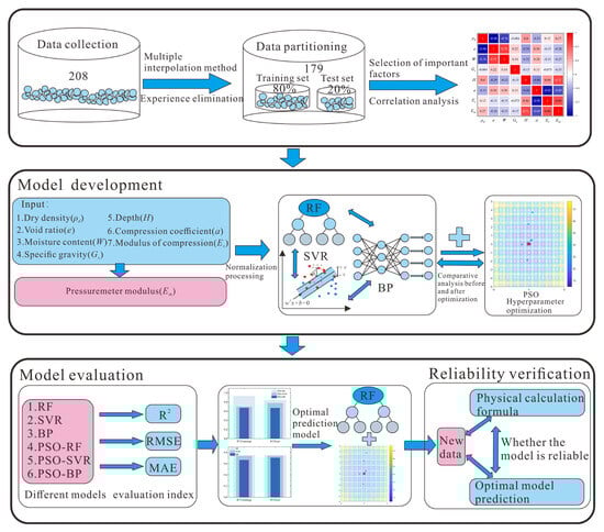
Figure 1.
The flowchart of the study on the prediction of the pressuremeter modulus.
Firstly, a total of 208 sets of physical and mechanical index samples were collected from different fine-grained sand layers within the site scope. These samples include wet density, dry density, void ratio, moisture content, specific gravity, relative density, depth, compression coefficient, compression modulus, cohesion, internal friction angle, and pressuremeter modulus, among other indices. After eliminating outliers and imputing missing data from these samples, a total of 179 sets of valid samples were collected. Parameters that have a certain influence on the pressuremeter modulus were selected as input parameters through Pearson correlation coefficient, thereby enhancing the accuracy of model prediction. Subsequently, after data standardization, the training set and test set were randomly divided at an 8:2 ratio. This study uses Support Vector Machine (SVR), Random Forest (RF), and BP Neural Network to predict the pressuremeter modulus of a deep overburden fine-grained sand layer, and will optimize the hyperparameters of the three models through Particle Swarm Optimization (PSO). The machine learning models are evaluated using Mean Absolute Error (MAE), Root Mean Square Error (RMSE), and coefficient of determination (R2) indicators. Finally, the soil layers that have not undergone the pressuremeter test are predicted using the machine learning model with the best predictive performance for the pressuremeter modulus. The results are then compared with those obtained from the pressuremeter modulus calculation formula based on physical mechanisms to verify the reliability of the proposed method.
4. Construction of the Database and Introduction to Different Machine Learning Models
4.1. Construction of the Database
4.1.1. Data Source and Probabilistic Statistical Analysis
Currently, due to the long history of deep overburden stratification in the dam site area of the southwest region, significant variations in soil layer properties, and complex stress–strain histories, their thickness generally exceeds 30 m. In one large hydropower project, the main foundation of the river-blocking dam is the ultra-deep overburden layer in the valley. The maximum depth of the overburden layer surpasses 500 m, with a thick layer of fine-grained sand serving as the primary bearing stratum for the hydropower station. This geological condition results in strong dispersion of rock and soil parameters in the region, which makes it difficult to study the correlation between various parameters and to provide an accurate basis for engineering construction. Therefore, it is necessary to conduct probabilistic statistics on the fine-grained sand layer parameters in this area. This study has compiled the original data of 208 soil samples based on existing field pressuremeter tests and indoor experiments. The dataset includes physical property indices such as wet density ρ, dry density ρd, void ratio e, moisture content W, specific gravity Gs, relative density Dr, and depth H, as well as mechanical property indices such as compression coefficient a, compression modulus Es, cohesion c, internal friction angle φ, and pressuremeter modulus Em. As shown in Figure 2, since the parameters are obtained according to the in situ tests and laboratory experiments, the data of other parameters except for relative density is relatively complete; therefore, the multiple imputation method is used to fill in the missing values of relative density. Figure 3 shows the comparison of box plots before and after the imputation of relative density. Due to errors in sampling and the experimental process, there are some outliers in the data, which reduce the accuracy and authenticity of the data and have a certain degree of impact on the accuracy of model predictions. Therefore, these factors should be fully considered when analyzing data. This paper eliminates some data with large deviations based on previous experience; ultimately, 179 sets of valid samples were obtained.
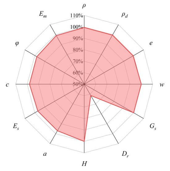
Figure 2.
Data completeness chart.
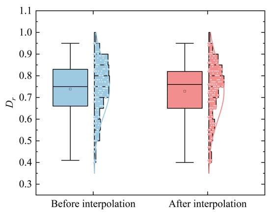
Figure 3.
Comparison of boxplots before and after relative density interpolation.
The statistical characteristics of various feature variables are shown in Table 1, which includes the maximum, minimum, mean, standard deviation, coefficient of variation, and 75th percentile values. It can be found that about 75% of the sampling depths were within 100 m. The average wet density and dry density of the sand layer are 1.92 g/cm3 and 1.64 g/cm3, respectively, with skewness values of 1.077 and −0.570 and kurtosis values of 0.132 and −0.093, indicating that the wet density data are overall right-skewed, while the dry density data has a relatively symmetrical distribution. The average value of the void ratio is 0.633, and the skewness and kurtosis values are −0.367 and 0.425, respectively, indicating that the void ratio data show a generally symmetrical distribution. The average value of the moisture content is 16.21%, and the skewness and kurtosis values are −1.328 and −0.357, respectively, indicating that the moisture content data are generally left-skewed. The average value of the specific gravity is 2.69, and the skewness and kurtosis values are 0.178 and 0.174, respectively, indicating that the specific gravity data are generally concentrated in terms of distribution. The average value of relative density is 0.72, and its skewness value and kurtosis value are −0.175 and 0.747, indicating that the relative density data present a symmetrical distribution; the average sampling depth is 79.63 m, and its skewness value and kurtosis value are 2.706 and 1.542, indicating that the depth data presents a right-skewed distribution. The average compression coefficient is 0.136 MPa−1, and its skewness value and kurtosis value are 3.167 and 1.149, indicating that the compression coefficient data are overall right-skewed. The average compressive modulus is 12.57 MPa, and its skewness value and kurtosis value are 0.443 and 0.469, indicating that the compressive modulus data are generally subject to a symmetric distribution. The average cohesion is 17.68 kPa, and its skewness value and kurtosis value are −0.948 and 0.359, indicating that the cohesion data are generally symmetrically distributed. The average value of internal friction angle is 29.31° and its skewness value and kurtosis value are 0.461 and −0.211, indicating that the data of internal friction angle is generally symmetrical. The average value of the pressuremeter modulus was 11.13 MPa, and its skewness value and kurtosis value were 0.116 and 0.249, respectively, indicating that the pressuremeter modulus data were generally symmetrically distributed. In addition, except for the moisture content and depth, the coefficients of variation in the physical indicators are relatively small, ranging from 1% to 20%. At the same time, it can be observed that the coefficients of variation for soil mechanical properties are generally greater than those for physical parameters.

Table 1.
Statistical summary of soil physical properties and mechanical parameters.
To more intuitively represent the distribution characteristics of geotechnical parameters, histograms of these parameters and fitting curves of normal distribution are drawn to display the overall appearance of data distribution. Simultaneously, the Q-Q plot is used to test the normal distribution of the data for this soil layer. Figure 4 shows the histograms of the distributions of each parameter and the corresponding Q-Q plots for this soil layer. It can be found that the data scatter of the remaining parameters, except for the depth and moisture content, basically follows the distribution along the diagonal line, indicating that it basically conforms to the approximately normal distribution. The histogram further shows that the data distribution of the depth parameter is relatively concentrated, while the moisture content is relatively dispersed due to the thick covering soil layer, with the moisture content of the soil body at different positions being mainly concentrated in the interval of about 25%. Based on the data shown in Table 1 above, the skewness values are mainly located in the range of −3 to +3, indicating that the symmetry of the data is acceptable; the kurtosis values are generally in the range of −10 to +10, indicating that the peak and distribution of the variables are at an acceptable level. Therefore, the sample data are relatively concentrated as a whole, basically conforming to the characteristics of normal distribution. The above analysis indicates that although the database only contains 179 sets of valid data, since the data essentially covers all depth ranges of the bearing sand layer and overall satisfies a normal distribution, the representativeness of the database is ensured. Through the representativeness and distribution characteristics of the data itself, a basic guarantee is provided for building a stable prediction model and reducing the risk of overfitting.
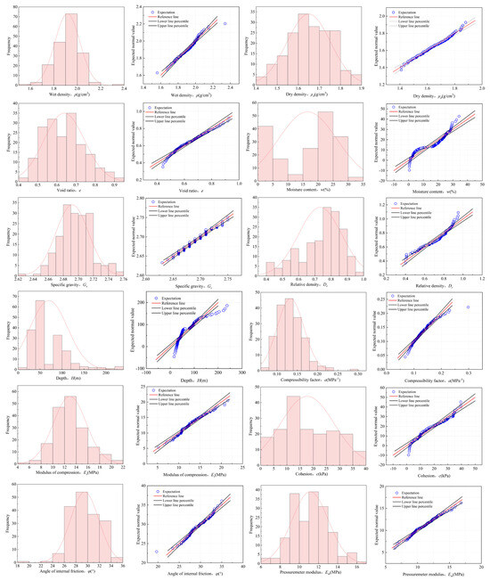
Figure 4.
Histograms of soil layer parameters and corresponding Q-Q plots.
4.1.2. Data Preprocessing
In the analysis and modeling process of soil parameters, normalization of variables can improve the reliability and accuracy of prediction models. The soil parameters included in this paper are mainly composed of physical property indices and mechanical property indices. Due to the significant difference in their dimensions, there is a large span in numerical ranges. If the original data are used for direct modeling, the order of magnitude differences between various parameters will affect the model’s sensitivity to data, as well as the training speed of machine learning. Normalization refers to the mathematical transformation that maps all parameters to a unified dimensional interval. By normalizing parameters, the gradient directions of various parameters can be balanced, making the optimization path smoother and significantly improving the efficiency of machine learning training.
Therefore, this paper employs min–max linear normalization to process the data, ensuring that the data are confined within the range of [0, 1] overall, thereby eliminating the difference in magnitude caused by different dimensions of various parameters. The linear normalization method is shown in Equation (1).
4.1.3. Correlation Analysis
Figure 5 presents the multivariate joint distribution map of various geotechnical parameters after screening, which displays the correlation and Pearson correlation coefficient among various geotechnical parameters in a manner of data visualization. When the correlation between datasets is very strong, the Pearson correlation coefficient r is ±0.81–±1, and similarly, the correlation coefficients for strong, moderate, and weak correlations between datasets are ±0.61–±0.8, ±0.41–±0.6, and ±0.21–±0.4, respectively; it can be seen from the figure that the distribution structure of all parameters is relatively concentrated. There is a strong correlation between dry density and void ratio (r = 0.98), and a strong correlation between compression coefficient and compression modulus (r = −0.91). This also indicates that the void ratio has a certain determining effect on the dry density, and the compression coefficient has a certain determining effect on the compression modulus. These parameters can be calculated by traditional calculation formulas and also reflect a strong correlation. In addition, there is a strong positive correlation between wet density and moisture content (r = 0.65) and a strong negative correlation between dry density and moisture content (r = −0.75). Moreover, there is a strong positive correlation between void ratio and moisture content (r = 0.75). Although there is a certain correlation between the remaining parameters (except for the pressuremeter modulus), they are all either moderately correlated or weakly correlated.
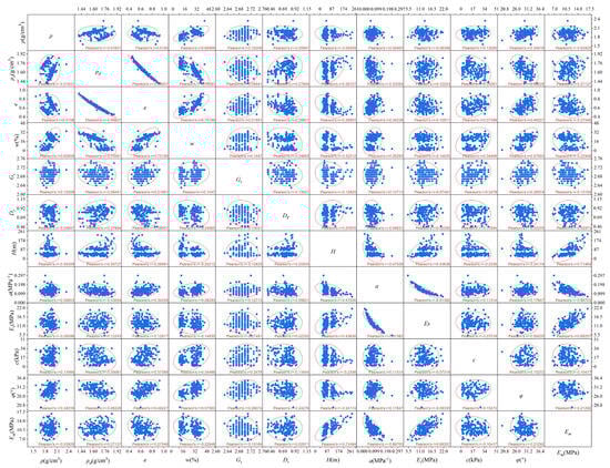
Figure 5.
Joint distribution diagram of multi-variables of geotechnical parameters.
In order to improve the accuracy of the model’s prediction of the pressuremeter modulus, this paper selects the correlation with the wet density ρ, dry density ρd, void ratio e, moisture content W, specific gravity Gs, relative density Dr, depth H, and mechanical property indices compression coefficient a, compression modulus Es, cohesion c, and internal friction angle φ. From Figure 5, it can be observed that there is a strong positive correlation (r = 0.71) between depth and pressuremeter modulus. The compression coefficient has a strong negative correlation with the pressuremeter modulus (r = −0.68) and the compression modulus has a strong positive correlation with the pressuremeter modulus (r = 0.68). The three factors of wet density, relative density, and cohesion show a weaker correlation with the pressuremeter modulus. In addition, due to the overall discrete data distribution between the internal friction angle and the pressuremeter modulus, it is not considered for selection. Therefore, this paper selects dry density, void ratio, moisture content, specific gravity, depth, compression coefficient, and compression modulus as the input variables x1, x2, x3, x4, x5, x6, x7, with the pressuremeter modulus as the output variable y.
To further analyze the correlation between individual input parameters and the output parameter, the pressuremeter modulus, a Pearson correlation coefficient heatmap was used for analysis and visualization. Figure 6 shows the correlation coefficient between the input parameters and the pressuremeter modulus, and it can be found that the results shown in the joint distribution diagram of multi-variables in the previous paper are not very different. Table 2 shows the significance p-value of the correlation coefficient between each input variable and the pressuremeter modulus. It can be found that the p-values are all less than 0.05 overall, indicating that the correlation coefficient between the input variables and the pressuremeter modulus is of certain significance. Figure 7 is the kernel density map between input variables and output variables, and it can be found that these input variables show a certain correlation with the pressuremeter modulus on the whole. The kernel density plots can better present the distribution pattern and range of these variables, providing insights into their potential influence on the pressuremeter modulus. Figure 7a shows that the dry density is mainly concentrated in 1.55–1.75 g/cm3, and it has a positive correlation with the pressuremeter modulus, and the pressuremeter modulus gradually increases as the dry density increases. Figure 7b shows that the void ratio is mainly concentrated in the range of 0.5–0.7 and is negatively correlated with the pressuremeter modulus. The modulus decreases gradually with the increase in the void ratio, which may be attributed to the fact that as the void ratio increases, the arrangement of particles to particles is looser, and the contact points are less, further causing the mechanical properties to decay. Figure 7c shows that the moisture content is mainly concentrated in the range of 15–30%, and it presents a negative correlation with the pressuremeter modulus. As the moisture content increases, the pressuremeter modulus gradually decreases. This may be attributed to the fact that at lower moisture contents, capillary tension occurs between particles, reducing the lubrication effect and improving the overall mechanical properties. Figure 7d shows that the specific gravity is mainly concentrated in the range of 2.65–2.70, and it has a certain negative correlation with the pressuremeter modulus. Figure 7e shows that the depth is mainly concentrated in the range of 0–150 m, and it has a certain positive correlation with the pressuremeter modulus. The pressuremeter modulus gradually increases as the depth increases, which may be attributed to the fact that as the depth increases in the same soil layer, the soil body as a whole is denser, and its deformation under the same pressure is smaller, making the mechanical properties better. Figure 7f shows that the compression coefficient is mainly concentrated in 0.10–0.15, which is negatively correlated with the pressuremeter modulus, and the pressuremeter modulus decreases gradually with the increase in the compression coefficient. Figure 7g shows that the compression modulus is mainly concentrated in the range of 5–16 MPa, and it has a strong positive correlation with the pressuremeter modulus. As the compression modulus increases, the pressuremeter modulus gradually increases. This may be attributed to the fact that the pressuremeter modulus comprehensively reflects the different performance of soil layers under tension and compression. Furthermore, for soil layers with little difference in mechanical properties between the vertical and horizontal directions, the gap between the pressuremeter modulus and the compression modulus is not significant, so the compression modulus has a certain influence on the pressuremeter modulus.
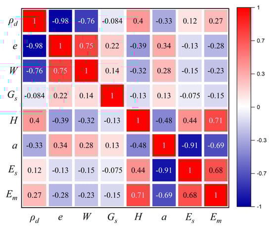
Figure 6.
Heatmap of correlations between input and output variables.
Table 2.
Significance of the correlation coefficients between input variables and the pressuremeter modulus p-value.
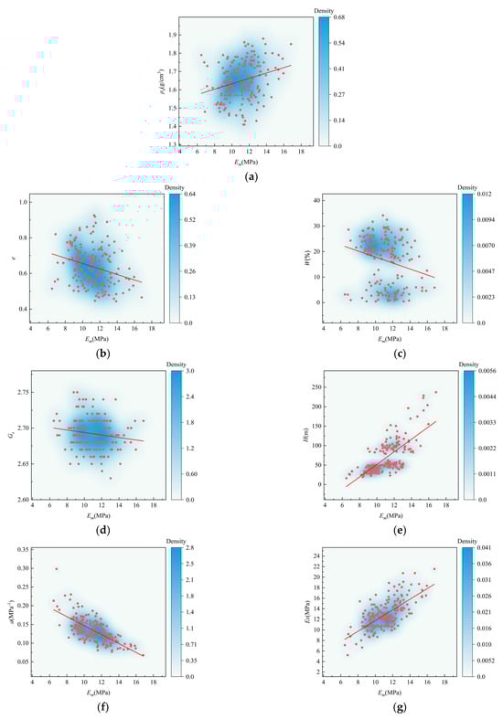
Figure 7.
Kernel density plot between input variables and output variables.
4.2. Introduction to the Basic Principles of Different Machine Learning Models
4.2.1. Random Forest (RF) Model
The random forest model is an ensemble learning algorithm and is an extended variant of Bagging. The core idea is to randomly extract multiple sample subsets from the original data with replacement. During the process of constructing each decision tree, the optimal feature is selected from the randomly extracted feature subset for splitting, ensuring the diversity of the decision trees. In regression problems, the prediction results are the average of the results from multiple decision trees. The number of decision trees, n, and the minimum sample size of the leaf nodes, leaf, are hyperparameters that have a certain impact on the predictive ability of the model. Due to the prediction of multiple decision trees, their prediction accuracy is usually extremely high. Randomly extracting subsets ensures that each tree has differences, thereby possessing strong anti-overfitting capabilities, and being able to evaluate feature importance. The downside is that the training and prediction speeds are relatively slow, and there is a possibility of overfitting for small data volumes or low-noise data [44]. The operation flow of the random forest model is shown in Figure 1.
4.2.2. Support Vector Regression (SVR) Model
Support Vector Machine (SVM) is a supervised learning model in machine learning with relevant learning algorithms, and it is generally referred to as SVR in regression problems. Its core idea is to find an optimal hyperplane that can separate data in high-dimensional feature space, and the classification equation of the hyperplane is represented as w·X + b = 0 [45]. In traditional linear regression models, the error loss is calculated by the difference between the model output f(x) and the actual value y. In the support vector machine model, the model is optimized by maximizing the margin width and minimizing the total loss; that is, allowing a maximum deviation of ε between f(x) and y. Losses are only calculated when this deviation exceeds ε. In practical problems, the hyperplane may be biased by some outliers, so the degree of deviation ε of the sample points is described by introducing slack variables and [46], transforming the original regression problem into the following:
which C denotes the penalty factor.
When there is a certain nonlinear relationship between parameters, a nonlinear function Φ(x) is often introduced, which is called the kernel function. Common kernel functions include the linear kernel function (Lin) and the Gaussian kernel function (RBF), among others. Support Vector Machines (SVM) are characterized by high memory efficiency, low computational cost, and strong predictive accuracy in high-dimensional spaces. Additionally, due to their focus on maximizing the margin, they can enhance the model’s generalization capability and reduce the risk of overfitting [47]. However, for large-scale samples, their training speed is slow, and the parameter setting of the kernel function has a significant impact on the accuracy of prediction. Due to its sensitivity to missing data and preprocessing, standardization must be performed before prediction. The operation flow of Support Vector Machine is shown in Figure 1.
4.2.3. BP Neural Network Model
The BP neural network is a supervised learning algorithm, formally known as the error backpropagation neural network. It is a classic feedforward neural network model, primarily characterized by two phases: forward propagation and error backpropagation.
The main structure of the BP neural network is divided into the input layer, hidden layer, and output layer; the hidden layer performs nonlinear transformations on the data, and the complexity of the network is determined by the number of hidden layers and the number of neurons in each layer. Its working principle mainly includes four stages: forward propagation, error calculation, backpropagation, and weight update [48]. The hidden layer and output layer are subjected to a nonlinear transformation through an activation function to obtain the output. The main activation functions include the log-sigmoid type function logsig, the tan-sigmoid type function tansig, and the linear function purelin type function. In regression models, sigmoid type functions are often used as the activation functions for hidden layer neurons [49]. The advantage of the BP neural network is that it has a strong nonlinear generalization ability, and it is highly self-learnable and fault-tolerant when there are sufficient training data and an appropriate network structure. Due to the use of the gradient descent method, the model training is slow and prone to falling into local minima; the model has a strong dependency on data, and when the amount of data is insufficient or the quality of data is not high, there is a certain risk of overfitting [50]. The simultaneous model is sensitive to hyperparameters such as network structure, learning rate, and initial weight. The BP neural network flowchart is shown in Figure 1.
4.2.4. Particle Swarm Optimization Algorithm
The Particle Swarm Optimization algorithm (PSO) is an evolutionary computation technique, the fundamental idea of which is to find the optimal solution through the collaboration and information sharing among individuals in the group. Each particle has its own position and velocity, moving within the search space influenced by the past individual best position pbest and the whole swarm best past position gbest. In each iteration update process, every particle updates its velocity and position based on the past individual optimal position and the global optimal position, with the entire particle swarm gradually converging to the optimal solution area in the search space [51]. The advantages are that the calculation speed is very fast, and it has strong global search capabilities for nonlinearity and multi-peaks. However, the disadvantages include a tendency to converge prematurely, i.e., falling into local optima, and poor local optimization capabilities [52]. A schematic diagram of the particle swarm algorithm is shown in Figure 1.
4.3. Evaluation Indicators of Model Prediction Performance
In order to quantitatively evaluate the predictive performance of machine learning models, this paper uses three regression prediction indicators: coefficient of determination (R2), root mean square error (RMSE), and mean absolute error (MAE) to assess model capabilities. These indicators have been validated in previous research.
The coefficient of determination R2 serves as a core metric for the ability to explain the data variation in models, reflecting the goodness of fit between predicted and actual values. The range of R2 values is generally between [0–1]. As R2 approaches 1, it indicates a better fitting effect. In Equation (5), the numerator represents the difference between the predicted set and the actual data, while the denominator represents the sum of squared differences between them.
The Root Mean Square Error (RMSE) is calculated by taking the difference between the actual and predicted values, averaging them, and then taking the square root. RMSE is sensitive to outliers and can reflect the volatility of the overall prediction bias. Generally, the smaller the RMSE value, the smaller the model error. It should be evaluated in conjunction with MAE (Mean Absolute Error) to comprehensively assess from the perspectives of volatility and stability. Equation (6) shows the calculation process of RMSE:
Mean Absolute Error (MAE) is an important indicator for model evaluation, which directly reflects the size of the absolute error between predicted and actual values, with a numerical range of [0, +∞]. The higher the value, the greater the error. Equation (7) shows the calculation process of MAE:
In the above formula, n represents the quantity of data, and and , respectively, denote the predicted values and actual values of the model.
5. Comparison and Discussion of the Prediction Results of the Pressuremeter Modulus of Deep Overburden
This section conducts input selection based on the parameters that exhibited good correlation with the pressuremeter modulus in the above text. The dry density ρd, void ratio e, moisture content W, specific gravity Gs, depth H, compression coefficient a, and compression modulus Es are used as feature values 1–7, respectively. This study adopts the holdout method in the model prediction process; in order to control the risk of overfitting in prediction and enhance the stability of model prediction, the data proportion is divided into a training set (80%) and a test set (20%) through random partitioning. Multiple evaluation metrics are employed to assess the predictive capabilities of the Random Forest (RF) model, Support Vector Regression model (SVR), and BP neural network model. Particle swarm optimization is utilized to optimize the hyperparameters of different models. Finally, the optimal predictive model is determined through comparative analysis of the performance of the optimized models. It should be noted that this study uniformly adopts the hold-out method instead of cross-validation mainly for the following reasons: First, Support Vector Regression (SVR) takes a long time to compute during the prediction process, and after hyperparameter optimization, its computational complexity is even higher. Second, the random partitioning method can improve computational efficiency while ensuring predictive performance. Third, for the Random Forest (RF) model and BP neural network, there is a certain randomness in their training process. This randomness makes it uncertain that multiple repeated training will necessarily reduce the error. Therefore, using a random partition hold-out method provides a benchmark for reasonably and consistently evaluating model performance.
5.1. RF Model Versus PSO-RF Model Prediction Results
Figure 8 shows the prediction results of the Random Forest (RF) computational model, in which the number of decision trees (trees) is set to 300, and the minimum number of samples at a leaf node (the minimum number of samples required at a leaf node) is 10. Figure 8a and Figure 8b, respectively, display the degree of coincidence between predicted and true values in the training set and test set. It can be observed that the overall deviation in both the training and test sets is relatively small, and the predicted values are close to the true values. Figure 8c and Figure 8d, respectively, show the scatter distribution of predicted values in the training set and the test set. The training set is more concentrated with the true values overall, while individual points in the test set deviate farther. Figure 8e shows the importance factors for the prediction of the pressuremeter modulus, and it can be found that the importance of the depth H, the compression coefficient a, and the compression modulus Es are relatively high compared to other factors. Figure 8f shows that as the number of decision trees increases, the overall error value decreases gradually, that is, the number of decision trees plays a certain role in reducing errors.
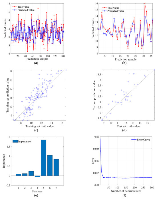
Figure 8.
RF model prediction result diagram: (a) training set prediction analysis; (b) test set prediction analysis; (c) training set prediction value scatter distribution; (d) test set prediction value scatter distribution; (e) factor importance; (f) error curve.
Figure 9 shows the prediction results of the Particle Swarm Optimization Random Forest (PSO-RF) model. The hyperparameters of the number of decision trees n and the minimum number of samples at leaf nodes in the Random Forest model are optimized through the Particle Swarm Optimization algorithm. The model sets the initial learning factors C1 (local search capability) and C2 (global search capability) to 1.4495 and sets the number of particle swarm algorithm population iterations to 120, with a population size of 5. The range of the optimal number of decision trees searched is [200–800], and the minimum leaf node sample number ranges from [1–7]. Finally, through the optimization of the particle swarm algorithm, the best hyperparameters obtained are n = 533 and leaf = 7.
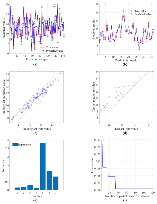
Figure 9.
PSO-RF model prediction result diagram: (a) training set prediction analysis; (b) test set prediction analysis; (c) training set prediction value scatter distribution; (d) test set prediction value scatter distribution; (e) factor importance; (f) fitness curve.
Figure 9a and Figure 9b, respectively, display the degree of coincidence between predicted and true values in the training set and test set. It can be observed that the overall deviation in the training dataset is relatively small, and the predicted values are close to the true values. The prediction results of the test set are basically consistent with the true values, indicating that the model has good generalization ability. Figure 9c and Figure 9d show the scatter distributions of predicted values in the training set and test set, respectively. The training set is more concentrated to the ground truth overall, and the test set data distribution deviates above the 45° reference line generally. Figure 9e shows the importance factors for the prediction of the pressuremeter modulus, and it can be found that the importance of the depth H, the compression coefficient a, and the compression modulus Es are higher compared to other factors. This is consistent with the results of the RF model. Figure 9f shows that the fitness value, i.e., the root mean square error value, decreases with the increase in the number of population iterations, and the fitness value basically converges when the number of iterations reaches about 40.
Figure 10 shows the values of different evaluation indicators for the training and test sets of RF and PSO-RF, as well as the comparison between the two models. It can be found that the R2 values for the training and testing sets of the RF model are 0.751 and 0.750, respectively, while those for the PSO-RF model are 0.930 and 0.840, respectively. The overall R2 values for both models are relatively high. The prediction results indicate that the RF model has a certain effect on the prediction of the pressuremeter modulus. Without hyperparameter tuning, the diversity of multiple decision trees enhances its resistance to overfitting, resulting in a decrease in prediction bias and volatility [44]. The fitting ability of the Random Forest model, after optimization by the particle swarm algorithm, has been further improved. In addition, the MAE of the RF model training set and test set were 0.750 and 0.679, respectively, while the MAE of PSO-RF model training set and test set were 0.392 and 0.606, respectively. The RMSE of the training and test sets were 0.960 and 0.819 for the RF model and 0.496 and 0.767 for the PSO-RF model. Based on the results of MAE and RMSE, it can be observed that after optimizing the hyperparameters of the Random Forest model through the Particle Swarm Optimization algorithm, the prediction error is relatively reduced, which somewhat enhances the accuracy of the predictions.
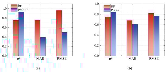
Figure 10.
Comparison of prediction evaluation indicators between RF and PSO-RF for training and test datasets: (a) training dataset; (b) test dataset.
5.2. Prediction Results of SVR Model and PSO-SVR Model
Figure 11 shows the prediction results of the SVR model. The penalty coefficient C and kernel parameter g of the model were set to 4.0 and 0.8, respectively. Figure 11a and Figure 11b, respectively, show the degree of coincidence between predicted and true values in the training set and test set. It can be observed that the deviation of predicted values in both the training and test sets is relatively small, demonstrating a certain predictive performance overall. Figure 11c and Figure 11d, respectively, display the scatter distribution of predicted values for the training set and test set. It can be observed that the deviation of predicted values for both the training and test sets has increased compared to the RF model, and overall, its predictive performance has declined.
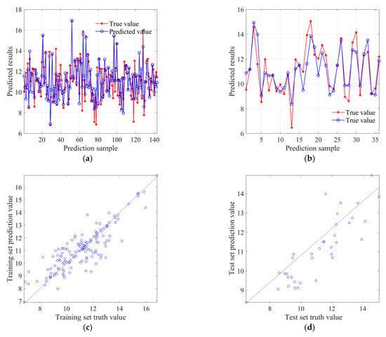
Figure 11.
SVR model prediction results: (a) training set prediction analysis; (b) test set prediction analysis; (c) scatter distribution of training set predicted values; (d) scatter distribution of test set predicted values.
Figure 12 shows the prediction results of the PSO-SVR model. Because the penalty coefficient C and kernel parameter g have a significant impact on the predictive ability of the SVR model, the particle swarm algorithm is used to find the optimal hyperparameters C and g for the SVR model. Set C1 and C2 to 1.5 and 1.7, respectively, the number of population iterations is 100, the population size is 10, and the search range for the penalty coefficient C and kernel parameter g is [0.1–100]. The optimal penalty coefficient C and kernel parameter g are finally obtained as 69.98 and 0.1, respectively.
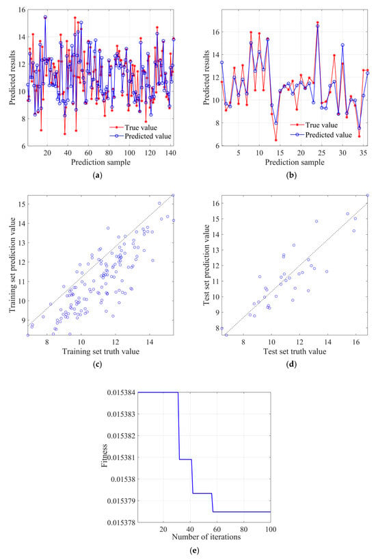
Figure 12.
PSO-SVR model prediction result diagram: (a) training set prediction analysis; (b) test set prediction analysis; (c) training set prediction value scatter distribution; (d) test set prediction value scatter distribution; (e) fitness curve.
Figure 12a and Figure 12b, respectively, show the degree of coincidence between predicted and true values in the training set and test set. It can be observed that the predicted values in both the training and test sets have improved compared to the SVR model, especially in the test set where a higher degree of coincidence between predicted and true values can be found. Figure 12c and Figure 12d, respectively, display the scatter distribution of predicted values for the training set and test set. It can be observed that the deviation of predicted values in the training set is more scattered compared to the SVR model, while the deviation of predicted values in the test set is less than that of the SVR model, with a more concentrated distribution. Figure 12e shows that the fitness value (root mean square error) decreases with the increase in the number of population iterations, and the fitness value basically converges around 60 times.
Figure 13 displays the values of different evaluation metrics for the training and testing sets of SVR and PSO-SVR, as well as the comparison between the two models. It can be observed that the R2 values for the SVR model’s training and testing sets are 0.737 and 0.742, respectively, while for the PSO-SVR model, they are 0.701 and 0.780. The overall R2 in both models is relatively high, reaching 0.7, indicating that the SVR model has a certain effect on the prediction of the pressuremeter modulus. Moreover, the prediction of the model is somewhat improved on the testing set through the particle swarm algorithm. It can also be observed that whether it is the SVR model or the PSO-SVR model, the R2 of the test set is higher than that of the training set, indicating that the models have good generalization capabilities. They are strong in predicting new data and possess a certain reliability for regression prediction under multi-feature factors. In addition, the MAE of SVR model training set and test set were 0.698 and 0.771, respectively, while that of PSO-SVR model training set and test set were 0.709 and 0.890, respectively. The RMSE of SVR model training set and test set were 0.962 and 0.992, while those of PSO-SVR model were 0.956 and 1.112. Based on the results of MAE and RMSE, it can be observed that after optimizing the hyperparameters of the SVR model through the particle swarm algorithm, the prediction error has relatively improved. This indicates that the validation model has overfitted the training data and exhibits a certain task dependency.
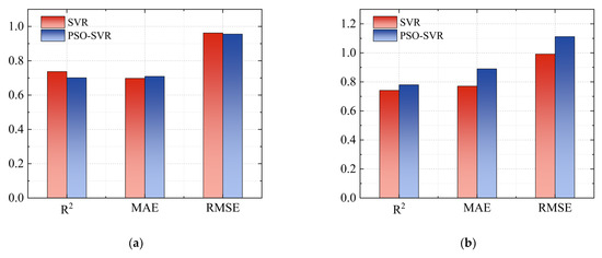
Figure 13.
Comparison of prediction evaluation indicators between SVR and PSO-SVR for training and test datasets: (a) training dataset; (b) test dataset.
5.3. BP Neural Network Model and PSO-BP Neural Network Model Prediction Results
Figure 14 presents the prediction results of the BP model. The number of neuron nodes in the input layer is set to 7, the hidden layer is 1 layer, the number of neuron nodes in the hidden layer is 9, and the number of neuron nodes in the output layer is 1. Figure 14a and Figure 14b, respectively, show the degree of coincidence between predicted and true values in the training set and test set. It can be observed that the deviation of predicted values on both the training and test sets is relatively small, demonstrating a certain level of predictive performance. However, compared to the RF model and the SVR model, its predictions have some deviation, indicating its limited predictive capability. Figure 14c and Figure 14d, respectively, display the scatter distribution of predicted values for the training set and test set. It can be observed that the deviation of the predicted values from the ideal prediction line for both the training and test sets has increased compared to the RF and SVR models. Overall, there has been a decline in its predictive performance. Figure 14e shows the change curve of mean absolute error with the number of training rounds, and it can be found that the optimal training round is twice, with an error value of 0.0182, and its subsequent curve changes are relatively stable.
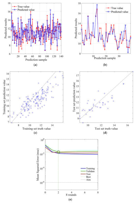
Figure 14.
BP neural network prediction results: (a) training set prediction analysis; (b) test set prediction analysis; (c) training set prediction value scatter distribution; (d) test set prediction value scatter distribution; (e) average absolute error change curve.
Figure 15 shows the prediction results of the PSO-BP neural network model. Since the initial weights W and thresholds B have a significant impact on the predictive ability of the BP neural network model, the particle swarm algorithm is used to find the optimal initial weights and thresholds for the BP neural network. Set C1 and C2 to 1.49 and 1.49, respectively, the population iteration times to 300, the population size to 10, and the maximum boundary range to [−5, 5]. Set the number of input neuron nodes to 7, the number of hidden layer neuron nodes to 9, the number of hidden layers to 1, and the number of output neuron nodes to 7.
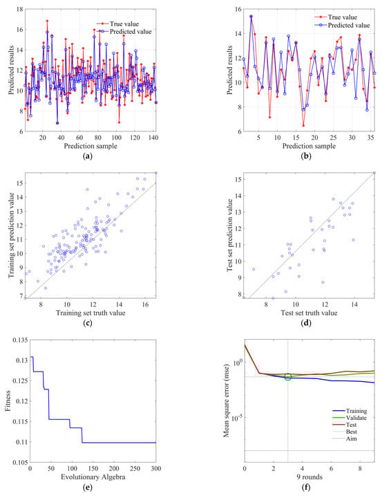
Figure 15.
PSO-BP neural network prediction results: (a) training set prediction analysis; (b) test set prediction analysis; (c) training set prediction value scatter distribution; (d) test set prediction value scatter distribution; (e) fitness change curve; (f) average absolute error change curve.
Figure 15a and Figure 15b, respectively, show the fit between predicted and true values in the training set and test set, and it can be found that the overall fitness is close to the BP neural network model. Figure 15c and Figure 15d, respectively, display the scatter distribution of predicted values in the training set and the test set. It can be observed that the deviation of predicted values in the training set is relatively more concentrated compared to the BP neural network model, while the degree of deviation in the test set is not significantly different from the BP neural network model. Figure 15e shows the decrease in fitness value (root mean square error) with the increase in population iteration times, where each iteration updates the weight only when the error of the validation set is less than or equal to the previous error, and the fitness value (root mean square error) basically converges at around 125 times. Figure 15f shows the change curve of mean absolute error with the training rounds, which can find that the best training round is three times, and the error value reaches 0.0458, and its subsequent curve changes smoothly.
Figure 16 shows the values of different evaluation indicators for the training and testing sets of the BP neural network model and the PSO-BP neural network model, as well as the comparison between the two models. It can be found that the R2 values of the training and testing sets for the BP neural network model are 0.665 and 0.705, respectively, while those for the PSO-BP neural network model are 0.675 and 0.672, respectively. The overall predictive performance of the two models is close, reaching above 0.65, but it is somewhat reduced compared to the predictive performance of the RF model and the SVR model, indicating that the predictive ability of the BP neural network model is limited. This may be attributed to the BP neural network being overly sensitive to hyperparameter tuning, where different hyperparameters have a significant impact on the predictive performance of the model [53], and also because of its high dependence on the number of data points, resulting in an overall weak fitting effect. In addition, the MAE of the BP neural network model training set and test set were 0.863 and 0.803, while the MAE of PSO-BP neural network model training set and test set were 0.834 and 0.923. The RMSE of the BP neural network model training set and test set were 1.085 and 1.024, while that of the PSO-BP neural network model were 1.057 and 1.165. It can be observed that after optimizing the hyperparameters of the BP neural network model through the particle swarm algorithm, the predictive performance of the training set has generally improved, and the error has relatively decreased. However, the overall effect on the test set has declined, indicating that the model’s generalization ability and stability are low, and there is a certain risk of overfitting.
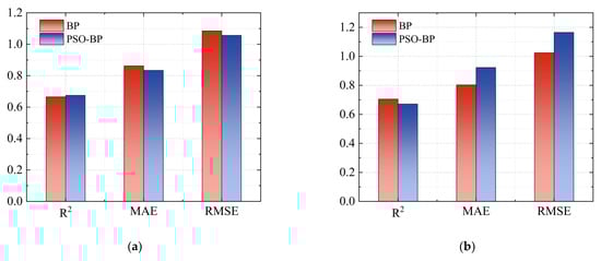
Figure 16.
Comparison of prediction evaluation indicators between BP and PSO-BP for training and test datasets: (a) training dataset; (b) test dataset.
5.4. Comparison and Analysis of Prediction Results from Different Machine Learning Models
Figure 17 and Table 3 show the comparison of evaluation indicators for different machine learning models. Figure 17a, Figure 17c, and Figure 17e display the comparison of evaluation indicators for the RF model, SVR model, and BP neural network model, respectively. It can be observed that the RF model exhibits the best predictive performance overall. In the predictions on the training set, its R2, MAE, and RMSE are 0.751, 0.750, and 0.960, respectively; in the test set, its R2, MAE, and RMSE are 0.750, 0.679, and 0.819, respectively. Overall, the model’s stability and error analysis are more precise compared to the SVR model and the BP neural network model. This might be attributed to the fact that the RF model is the result of multiple decision trees making predictions together. This diversity enhances predictive performance. In addition, the sensitivity of the RF model to hyperparameters is relatively lower compared to the SVR model and BP neural network, making it more robust [54]. It has a certain reliability in establishing the relationship between soil physical and mechanical parameters [55].
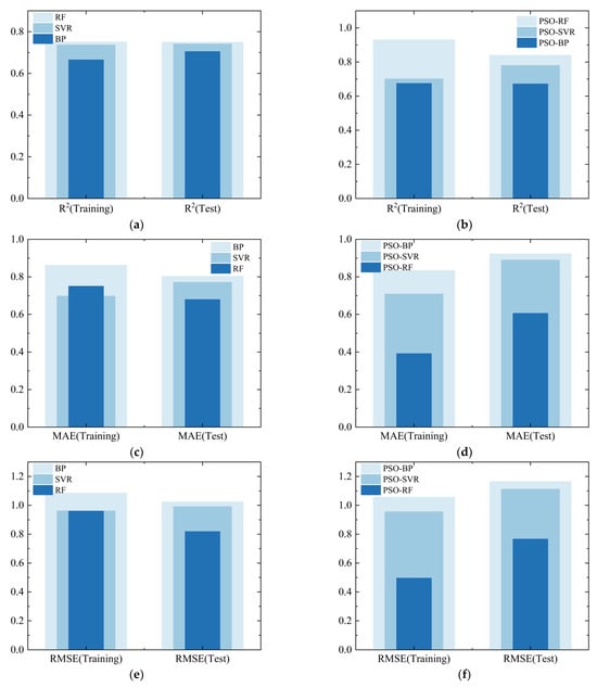
Figure 17.
Comparison of the performance of different machine learning models: (a) R2 comparison of RF, SVR, BP models; (b) R2 comparison of PSO-RF, PSO-SVR, PSO-BP models; (c) MAE comparison of RF, SVR, BP models; (d) MAE comparison of PSO-RF, PSO-SVR, PSO-BP models; (e) RMSE comparison of RF, SVR, BP models; (f) RMSE comparison of PSO-RF, PSO-SVR, PSO-BP models.
Table 3.
Comparison of evaluation metrics for different machine learning models.
Figure 17b, Figure 17d, and Figure 17f, respectively, display the comparison of evaluation indicators for the PSO-RF model, PSO-SVR model, and PSO-BP neural network model. It can be observed that after optimization through the particle swarm algorithm, the RF and SVR models generally exhibit better performance, while the performance of the BP neural network model is average. This might be attributed to the particle swarm algorithm falling into a local optimal solution, thereby leading to the optimal weights and thresholds searched not significantly enhancing the predictive capability of the BP neural network, also indirectly reflecting the strong sensitivity of the BP neural network to initial weights and thresholds. The R2 values of the training set for PSO-RF, PSO-SVR, and PSO-BP are 0.930, 0.701, and 0.675, respectively, while the R2 values of the test set are 0.840, 0.780, and 0.672, respectively. This indicates that the optimized RF model has a stronger fitting capability. From the error analysis, it can be seen that the MAE and RMSE of the test set for the PSO-RF model are 0.606 and 0.767, respectively. Compared to the PSO-SVR model, they have been reduced by 46.91% and 44.98%, respectively, and compared to the PSO-BP model, they have been reduced by 52.36% and 51.89%, respectively. This suggests that the PSO-RF model has a greater advantage in controlling errors when predicting new data compared to PSO-SVR and PSO-BP. Taken together, it indicates the comprehensive superiority of the RF model and PSO-RF model in the task of predicting the parameters of the pressuremeter modulus.
6. Reliability Verification of the Physical Mechanism of the Pressuremeter Modulus of Deep Overburden
In order to verify the accuracy of the established optimal prediction model in practical applications, this paper collects five sets of new data that have not undergone pressuremeter tests and uses the optimal machine learning model to predict the pressuremeter modulus of these five sets of data. In order to further verify the reliability of the model, a comparison analysis based on physical mechanisms was conducted to verify the consistency between the machine learning prediction results and theoretical values.
Yu Haisui [56] pointed out that the pressuremeter test is essentially the expansion of a long cylindrical membrane placed in the soil, so the results of the pressuremeter test can be explained by the cavity expansion methods in geomechanics. When the cylindrical hole wall is subjected to an additional uniform pressure △P (△P = P − P0, where P is the pressure acting on the hole wall, P0 is the original horizontal stress of the soil body), a displacement u will occur at the point with a radius of r around the hole wall. The corresponding elastic analytical expression can be obtained by assuming plane strain theory to conduct an elastic analysis of the cylinder expansion [56]:
where u is the displacement at radius a, G is the shear modulus at that point, and represent the radial stress and tangential stress at that point, respectively. Due to , the horizontal modulus, i.e., the pressuremeter modulus, can be solved.
From the analytical expression, it can be observed that the determination of the pressuremeter modulus is closely related to the slope of the linear segment of the pressuremeter curve. Meanwhile, the deformation modulus of the soil obtained through field load tests is also derived from the slope of the soil’s linear segment. Therefore, there must be some connection between the two. Then, since the pressuremeter modulus Em can comprehensively reflect the different performance of the soil layer in tension and compression, while the deformation modulus E0 mainly reflects the compression performance in the vertical direction, the two are not completely equivalent. Under general engineering geological conditions, the difference between Em and E0 of soil mass is less than 5%. Meanwhile, when the mechanical properties of the soil layer show significant anisotropy in two directions, the difference between the two will gradually increase. Overall, Em < E0.
To establish the relationship between the deformation modulus E0 and the pressuremeter modulus Em, Menard [8] linked the two through a large amount of comparative data analysis and introduced the soil structure coefficient α, which reflects the rheological properties of the soil body and its stress history. This coefficient changes with the type of soil, stress history, and location. Through numerous pressuremeter tests, Menard further established a correlation between α and the core parameters of the pressuremeter test, Em and Pl. That is, α is a function of the soil type and the ratio of Em/Pl. This provides a theoretical basis and practical method for predicting the pressuremeter modulus, as shown in Equation (11). Table 4 shows common values of α for sandy soils.
Table 4.
Common values of α for sand.
In addition, based on the assumption of linear elasticity theory, the theoretical relationship between the deformation modulus E0 and the compression modulus Es can be derived, as shown in Equation (12). Equation (13) reflects the close relationship between Es and the initial void ratio e and compression coefficient a of the soil body. From this, it can be inferred that there is a close relationship between the pressuremeter modulus and the void ratio e, and the compression modulus Es. This also provides a physical explanation for the parameters selected for predicting the pressuremeter modulus in the machine learning model discussed above.
Since the derivation of Equation (12) is based on the generalized Hooke’s law, it assumes that the soil body is a linear elastic body during the loading process and meets ideal conditions such as isotropy and continuous homogeneous medium. However, the deep overburden soil properties in the study area are complex. Due to the sedimentary environment, consolidation degree, and stress history, they exhibit significant anisotropy and non-homogeneity as a whole. They cannot be simply assumed to be a continuous homogeneous medium. Furthermore, Es is measured through indoor confined compression tests, with a stress range of 0.1–0.2 MPa, which difficultly reflects the actual deformation characteristics of the vertical direction in deep overburden layers. On the other hand, the deformation modulus E0 is taken from the linear segment of the P-S curve in field load tests, where its stress level is generally higher, resulting in E0 being greater than Es. Therefore, considering the significant differences between the actual conditions mentioned above and theoretical assumptions, it is difficult to deduce the deformation modulus representing the actual working state in the field from the compression modulus obtained through indoor confined compression tests. Using Equation (12) for derivation will lead to significant errors. Therefore, Equation (11) proposed by Menard is directly used for the prediction of the pressuremeter modulus.
After calculation, the values of Em/Plm for this soil layer are mainly concentrated in the range of 7–12. Through consolidation characteristic tests on the undisturbed sand samples from the site, it was found that the bearing sand layer is generally normally consolidated and slightly over-consolidated. Therefore, based on the values of Em/Plm and the state of the sand layer, α is set to 0.33. Table 5 lists the physical property indices and mechanical property parameters corresponding to the soil layers within 100 m without pressuremeter tests in five groups.
Table 5.
Basic physical and mechanical parameters of soil strata without pressuremeter test.
Figure 18 and Table 6 display the comparison of prediction results through Menard’s calculation formula, the RF model, and the PSO-RF model under the setting of α = 0.33. It can be found that, with the calculation results proposed by Menard as the benchmark values, both the RF model and PSO-RF model demonstrate a good level of reliability. Among them, the RMSE of RF is 0.422, R2 is 0.752, while the RMSE of PSO-RF is 0.173, and R2 is 0.958. By comparison, it can be found that the predicted pressuremeter modulus of PSO-RF for these five groups of soils is closer to the results calculated by the Menard formula, and the prediction error is relatively small, which can be attributed to the significant optimization effect of the particle swarm algorithm on the hyperparameters of the RF model. Through the Pearson correlation coefficient r, it can be found that the predicted values of both models have a high correlation with the results calculated using the formula proposed by Menard, reaching 98.8 and 99.3, respectively. Moreover, the p-values are both much less than 0.05, indicating that the correlation coefficients are statistically significant. This indicates that the predictions of the two models within a depth of 100 are reliable on the whole.
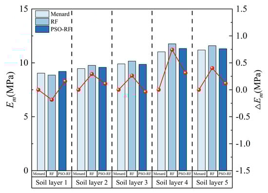
Figure 18.
Reliability verification of prediction results by the RF model and PSO-RF model.
Table 6.
Comparison of RF model and PSO-RF model prediction results with Menard calculation formula.
7. Conclusions
This paper takes the deep sand layer of the riverbed foundation of a proposed large hydropower project dam in the southwest region of China as the research object. It systematically collects key physical and mechanical parameters, including dry density, void ratio, moisture content, specific gravity, depth, compression coefficient, compression modulus, and pressuremeter modulus, to construct a sand layer parameter database. Based on this, a data-driven method is proposed to analyze the relationship between the conventional physical and mechanical parameters of sandy soil layers and the pressuremeter modulus. In the study, three machine learning algorithms, namely Random Forest (RF), Support Vector Regression (SVR), and BP Neural Network, were employed to construct prediction models for the pressuremeter modulus of sandy soil layers. The hyperparameters of these three models were optimized using the Particle Swarm Optimization (PSO) algorithm to enhance their predictive performance. Through comparative evaluation, the best predictive model was determined. Finally, a reliability analysis was conducted in conjunction with the physical mechanism calculation formulas. This paper reached the following conclusions:
- (1)
- Through the correlation analysis and p-value detection between the conventional physical and mechanical parameters of the sandy soil layer and the pressuremeter modulus, it was found that the dry density ρd, void ratio e, moisture content W, specific gravity Gs, depth H, compression coefficient a, and compression modulus Es have a certain correlation with the pressuremeter modulus Em. Furthermore, the correlation of depth H, compression coefficient a, and compression modulus Es with it is significant.
- (2)
- In the prediction of the pressuremeter modulus of sandy soil layers by Random Forest (RF), Support Vector Regression (SVR), and BP Neural Network, the RF model demonstrates the strongest prediction accuracy and stability. In the training set, its R2, MAE, and RMSE are 0.751, 0.750, and 0.960, respectively, while in the test set, its R2, MAE, and RMSE are 0.750, 0.679, and 0.819, respectively, showcasing the strongest fitting ability and error control capability. Additionally, it was found that the three parameters of depth H, compression coefficient a, and compression modulus Es are of the highest importance to the pressuremeter modulus Em.
- (3)
- After optimizing the hyperparameters of Random Forest (RF), Support Vector Machine (SVR), and BP Neural Network using Particle Swarm Optimization (PSO), the predictive performance of Random Forest (RF) and Support Vector Machine (SVR) improved, while the overall changes in the BP Neural Network were not significant. Among them, the Random Forest model exhibited the most comprehensive predictive performance after hyperparameter optimization. In the training set, its R2, MAE, and RMSE were 0.930, 0.392, and 0.496, respectively. In the test set, its R2, MAE, and RMSE were 0.840, 0.606, and 0.767, respectively.
- (4)
- For sandy soil layers without pressuremeter tests, the RMSE and R2 between the results of the pressuremeter modulus predicted by the RF model and the Menard calculation results under the setting of α = 0.33 are 0.422 and 0.752, respectively. The RMSE and R2 between the results of the pressuremeter modulus predicted by the PSO-RF model and the Menard calculation results under the setting of α = 0.33 are 0.173 and 0.958, respectively, with r values of 98.8 and 99.3 and P values all far less than 0.05, showing good correlation overall. This indicates that the prediction of the pressuremeter modulus through the RF model and PSO-RF model has certain reliability.
Although this study verifies that the RF model and PSO-RF model have reliable prediction capabilities for the pressuremeter modulus of a deep overburden sand layer in the main valley of a proposed large hydropower project’s barrage dam foundation in Southwest China, there are still several limitations and shortcomings. Firstly, although the dataset of the deep overburden sandy soil layer parameters obtained in this study has a certain representativeness and distribution rationality, the effective data sample size is still small, with 75% of the data concentrated within the range of 100 m. This leads to an inability to comprehensively and completely reflect the characteristics of the deeper sandy soil layers in the region. This restricts the universality of the model and carries a certain risk of overfitting, affecting the reliability of the model’s extension to deeper layers. Secondly, this paper only collected the relevant parameters of the deep overburden sand layer in the main valley of the foundation of a large hydropower project dam under construction, which also results in certain regional limitations of the developed prediction model. The geological conditions in the southwest region are complex and diverse, which makes it impossible to make robust predictions and generalizations for the deep overburden-bearing strata in the entire southwest region. Thirdly, this paper does not carry out multiple verification strategies, such as K-fold cross-validation, in the prediction validation aspect, which may affect the robustness of model performance evaluation. Finally, the new dataset used for reliability verification, which includes deformation modulus, is limited, and a single structural coefficient α cannot fully represent the properties of the entire sand layer, which is insufficient for stably verifying the reliability of the model.
In future research, the focus will be on the following aspects: first, a broader range of data samples will be integrated, especially increasing the effective data beyond 100 m depth, in order to enhance the completeness and representativeness of the database, reduce the predictive risk of the model, and expand the model’s adaptability and generalization capabilities. In particular, by collecting more field load test data that includes deformation modulus, and systematically considering the effects of different consolidation degrees, stress paths, and testing methods on α, we can determine a reasonable range of α coefficients applicable to this bearing sand layer. By statistically analyzing the proportion of model prediction results within this range, we can more accurately and objectively evaluate the reliability of the prediction model. Secondly, the model is applied to other engineering cases in the southwest region of China to test its performance under different geological and engineering conditions, in order to enhance the universality and practical value of the model in engineering. Another important direction is to adopt nested K-fold cross validation and repeated cross validation in the prediction process, and design nested cross validation for hyperparameter tuning, so as to obtain more statistically significant performance metrics, thus building a more stable prediction model.
Author Contributions
H.G.: conceptualization, methodology, software, data curation, formal analysis, investigation, writing—original draft preparation; D.C.: conceptualization, validation, investigation, resources, writing—review and editing, supervision, funding acquisition; Q.L.: investigation, visualization, validation, Q.C.: investigation, visualization, supervision, L.L.: software, supervision. All authors have read and agreed to the published version of the manuscript.
Funding
This study is supported by the National Natural Science Foundation of China [Grant No. 42277171].
Institutional Review Board Statement
Not applicable.
Informed Consent Statement
Not applicable.
Data Availability Statement
The data presented in this study are available on request from the author.
Conflicts of Interest
Author Qingchun Li was employed by the company “Chengdu Engineering Corporation Limited, Chengdu”. The remaining authors declare that the research was conducted in the absence of any commercial or financial relationships that could be construed as a potential conflict of interest.
Abbreviations
The following abbreviations are used in this manuscript:
| RF | Random Forest model |
| PSO-RF | Particle Swarm Optimization Random Forest model |
| SVR | Support Vector Regression model |
| PSO-SVR | Particle Swarm Optimization Support Vector Regression model |
| BP | BP Neural Network |
| PSO-BP | Particle Swarm Optimization BP Neural Network |
References
- Yu, T.; Shao, L. Study on the dynamic characteristics of dam foundation on deep riverbed overburden with soft soil layer. Rock Soil Mech. 2020, 41, 267–277. [Google Scholar]
- Zhou, X.; He, Y.; Zhao, R. Seismic safety evaluation of foundation gallery of rockfill dam on deep overburden. Eng. J. Wuhan Univ./Wuhan Daxue Xuebao 2012, 45, 447–453. [Google Scholar]
- Luo, Y.L.; Zhang, X.J.; Zhang, H.B.; Sheng, J.C.; Zhan, M.L.; Wang, H.M.; He, S.Y. Review of suffusion in deep alluvium foundation. Rock Soil Mech. 2022, 2022, 3094–3106. [Google Scholar]
- Zhang, S.; Li, Q.; Liu, S.; Cui, D.; Li, H.; Li, W.; Chen, P. A state-of-the-art review on the borehole in-situ testing techniques in deep overburden layer. Rock Soil Mech. 2025, 1–20. [Google Scholar]
- Kang, J.; Deng, G.; Kang, Z. Strength classification and evaluation method for saturated loess using pressuremeter test method. Rock Soil Mech. 2024, 45, 557–567. [Google Scholar]
- Agan, C. Determination of the deformation modulus of dispersible-intercalated-jointed cherts using the Menard pressuremeter test. Int. J. Rock Mech. Min. Sci. 2014, 65, 20–28. [Google Scholar] [CrossRef]
- Kayabasi, A. Prediction of pressuremeter modulus and limit pressure of clayey soils by simple and non-linear multiple regression techniques: A case study from Mersin, Turkey. Environ. Earth Sci. 2012, 66, 2171–2183. [Google Scholar] [CrossRef]
- Baud, J.P. Analyse des résultats pressiométriques Ménard dans un diagramme spectral [Log (pLM), Log (EM/pLM)] et utilisation des regroupements statistiques dans la modélisation d’un site. ISP5–PRESSIO 2005, 1, 167–174. [Google Scholar]
- Goh, K.H.; Jeyatharan, K.; Wen, D. Understanding the stiffness of soils in Singapore from pressuremeter testing. Geotech. Eng. J. SEAGS AGSSEA 2012, 43, 56–62. [Google Scholar]
- Biarez, J.; Gambin, M.; Gomes-Correia, A.; Flavigny, E.; Branque, D. Using Pressuremeter to Obtain Parameters to Elastic-Plastic Models for Sands; A.A. Balkema Brookfield: Rotterdam, The Netherlands, 1998. [Google Scholar]
- Fawaz, A.; Hagechehade, F.; Farah, E. A study of the pressuremeter modulus and its comparison to the elastic modulus of soil. Study Civ. Eng. Archit. SCEA 2014, 3, 7–15. [Google Scholar]
- Bardhan, A.; Samui, P. Probabilistic slope stability analysis of Heavy-haul freight corridor using a hybrid machine learning paradigm. Transp. Geotech. 2022, 37, 100815. [Google Scholar] [CrossRef]
- Gao, W.; Raftari, M.; Rashid, A.S.A.; Mu Azu, M.A.; Jusoh, W.A.W. A predictive model based on an optimized ANN combined with ICA for predicting the stability of slopes. Eng. Comput. 2020, 36, 325–344. [Google Scholar] [CrossRef]
- Ahangari Nanehkaran, Y.; Pusatli, T.; Chengyong, J.; Chen, J.; Cemiloglu, A.; Azarafza, M.; Derakhshani, R. Application of machine learning techniques for the estimation of the safety factor in slope stability analysis. Water 2022, 14, 3743. [Google Scholar] [CrossRef]
- Zhang, W.; Gu, X.; Tang, L.; Yin, Y.; Liu, D.; Zhang, Y. Application of machine learning, deep learning and optimization algorithms in geoengineering and geoscience: Comprehensive review and future challenge. Gondwana Res. 2022, 109, 1–17. [Google Scholar] [CrossRef]
- Aouadj, A.; Bouafia, A. CPT-based method using hybrid artificial neural network and mathematical model to predict the load-settlement behaviour of shallow foundations. Geomech. Geoengin. 2022, 17, 321–333. [Google Scholar] [CrossRef]
- Sasmal, S.K.; Behera, R.N. Transient settlement estimation of shallow foundation under eccentrically inclined static and cyclic load on granular soil using artificial intelligence techniques. Geomech. Geoengin. 2023, 18, 560–576. [Google Scholar] [CrossRef]
- Zhang, N.; Zhou, A.; Pan, Y.; Shen, S. Measurement and prediction of tunnelling-induced ground settlement in karst region by using expanding deep learning method. Measurement 2021, 183, 109700. [Google Scholar] [CrossRef]
- Erharter, G.H.; Marcher, T.; Reinhold, C. Artificial Neural Network Based Online Rockmass Behavior Classification of Tbm Data; Springer: Berlin/Heidelberg, Germany, 2019. [Google Scholar]
- Ling, J.; Li, X.; Li, H.; Shen, Y.; Rui, Y.; Zhu, H. Data acquisition-interpretation-aggregation for dynamic design of rock tunnel support. Autom. Constr. 2022, 143, 104577. [Google Scholar] [CrossRef]
- Liu, J.; Jiang, Y.; Han, W.; Sakaguchi, O. Optimized ANN model for predicting rock mass quality ahead of tunnel face using measure-while-drilling data. Bull. Eng. Geol. Environ. 2021, 80, 2283–2305. [Google Scholar] [CrossRef]
- Bardhan, A.; Kardani, N.; Alzo'Ubi, A.K.; Roy, B.; Samui, P.; Gandomi, A.H. Novel integration of extreme learning machine and improved Harris hawks optimization with particle swarm optimization-based mutation for predicting soil consolidation parameter. J. Rock Mech. Geotech. Eng. 2022, 14, 1588–1608. [Google Scholar] [CrossRef]
- Mohammadzadeh, D.; Bazaz, J.B.; Alavi, A.H. An evolutionary computational approach for formulation of compression index of fine-grained soils. Eng. Appl. Artif. Intell. 2014, 33, 58–68. [Google Scholar] [CrossRef]
- Kalantary, F.; Kordnaeij, A. Prediction of compression index using artificial neural network. Sci. Res. Essays 2012, 7, 2835–2848. [Google Scholar] [CrossRef]
- Nguyen, B.; Nguyen, T.; Le, V. An advanced machine learning-based mathematical equation for predicting compression index from readily-available soil physical properties. Geomech. Geoengin. 2025, 20, 1–17. [Google Scholar] [CrossRef]
- Ehsan, M.; Manzoor, U.; Chen, R.; Hussain, M.; Abdelrahman, K.; Radwan, A.E.; Ullah, J.; Iftikhar, M.K.; Arshad, F. Pore pressure prediction based on conventional well logs and seismic data using an advanced machine learning approach. J. Rock Mech. Geotech. Eng. 2025, 17, 2727–2740. [Google Scholar] [CrossRef]
- Ziaie Moayed, R.; Kordnaeij, A.; Mola-Abasi, H. Pressuremeter modulus and limit pressure of clayey soils using GMDH-type neural network and genetic algorithms. Geotech. Geol. Eng. 2018, 36, 165–178. [Google Scholar] [CrossRef]
- Moayedi, H.; Gör, M.; Khari, M.; Foong, L.K.; Bahiraei, M.; Bui, D.T. Hybridizing four wise neural-metaheuristic paradigms in predicting soil shear strength. Measurement 2020, 156, 107576. [Google Scholar] [CrossRef]
- Tizpa, P.; Jamshidi Chenari, R.; Karimpour Fard, M.; Lemos Machado, S. ANN prediction of some geotechnical properties of soil from their index parameters. Arab. J. Geosci. 2015, 8, 2911–2920. [Google Scholar] [CrossRef]
- Khatti, J.; Grover, K.S. Prediction of compaction parameters for fine-grained soil: Critical comparison of the deep learning and standalone models. J. Rock Mech. Geotech. Eng. 2023, 15, 3010–3038. [Google Scholar] [CrossRef]
- Zheyuan, F.; Cheng, C.; Manman, D.; Pengjiao, J. A Deep Learning Model for Predicting the Cement Soil Deformation Modulus. Langmuir 2025, 41, 21878–21889. [Google Scholar] [CrossRef]
- Liu, C.; Ku, C.; Wu, T.; Ku, Y. An Advanced Soil Classification Method Employing the Random Forest Technique in Machine Learning. Appl. Sci. 2024, 14, 7202. [Google Scholar] [CrossRef]
- Pham, B.T.; Qi, C.; Ho, L.S.; Nguyen-Thoi, T.; Al-Ansari, N.; Nguyen, M.D.; Nguyen, H.D.; Ly, H.; Le, H.V.; Prakash, I. A novel hybrid soft computing model using random forest and particle swarm optimization for estimation of undrained shear strength of soil. Sustainability 2020, 12, 2218. [Google Scholar] [CrossRef]
- Ly, H.; Thai Pham, B. Soil unconfined compressive strength prediction using random forest (RF) machine learning model. Open Constr. Build. Technol. J. 2020, 14, 278–285. [Google Scholar] [CrossRef]
- Ma, G.; Chao, Z.; Zhang, Y.; Zhu, Y.; Hu, H. The Application of Support Vector Machine in Geotechnical Engineering; IOP Publishing: Bristol, UK, 2018. [Google Scholar]
- Kirts, S.; Nam, B.H.; Panagopoulos, O.P.; Xanthopoulos, P. Settlement prediction using support vector machine (SVM)-based compressibility models: A case study. Int. J. Civ. Eng. 2019, 17, 1547–1557. [Google Scholar] [CrossRef]
- Zhao, H.; Yin, S. Geomechanical parameters identification by particle swarm optimization and support vector machine. Appl. Math. Model. 2009, 33, 3997–4012. [Google Scholar] [CrossRef]
- Cui, K.; Jing, X. Research on prediction model of geotechnical parameters based on BP neural network. Neural Comput. Appl. 2019, 31, 8205–8215. [Google Scholar] [CrossRef]
- Hajihassani, M.; Jahed Armaghani, D.; Kalatehjari, R. Applications of particle swarm optimization in geotechnical engineering: A comprehensive review. Geotech. Geol. Eng. 2018, 36, 705–722. [Google Scholar] [CrossRef]
- Suescun-Florez, E.; Roslyakov, S.; Iskander, M.; Baamer, M. Geotechnical properties of BP-1 lunar regolith simulant. J. Aerosp. Eng. 2015, 28, 4014124. [Google Scholar] [CrossRef]
- Yin, Z.Y.; Jin, Y.F.; Shen, J.S.; Hicher, P.Y. Optimization techniques for identifying soil parameters in geotechnical engineering: Comparative study and enhancement. Int. J. Numer. Anal. Methods Geomech. 2018, 42, 70–94. [Google Scholar] [CrossRef]
- Nama, S.; Saha, A.K.; Ghosh, S. Parameters optimization of geotechnical problem using different optimization algorithm. Geotech. Geol. Eng. 2015, 33, 1235–1253. [Google Scholar] [CrossRef]
- Kashani, A.R.; Chiong, R.; Mirjalili, S.; Gandomi, A.H. Particle swarm optimization variants for solving geotechnical problems: Review and comparative analysis. Arch. Comput. Methods Eng. 2021, 28, 1871–1927. [Google Scholar] [CrossRef]
- Salman, H.A.; Kalakech, A.; Steiti, A. Random forest algorithm overview. Babylon. J. Mach. Learn. 2024, 2024, 69–79. [Google Scholar] [CrossRef]
- Cemiloglu, A.; Zhu, L.; Arslan, S.; Xu, J.; Yuan, X.; Azarafza, M.; Derakhshani, R. Support vector machine (SVM) application for uniaxial compression strength (UCS) prediction: A case study for Maragheh limestone. Appl. Sci. 2023, 13, 2217. [Google Scholar] [CrossRef]
- Wang, W.; Chau, K.; Cheng, C.; Qiu, L. A comparison of performance of several artificial intelligence methods for forecasting monthly discharge time series. J. Hydrol. 2009, 374, 294–306. [Google Scholar] [CrossRef]
- Shao, W.; Yue, W.; Zhang, Y.; Zhou, T.; Zhang, Y.; Dang, Y.; Wang, H.; Feng, X.; Chao, Z. The application of machine learning techniques in geotechnical engineering: A review and comparison. Mathematics 2023, 11, 3976. [Google Scholar] [CrossRef]
- Cao, W.; Jiang, Y.; Sakaguchi, O.; Li, N.; Han, W. Predication of displacement of tunnel rock mass based on the back-analysis method-BP neural network. Geotech. Geol. Eng. 2022, 40, 531–544. [Google Scholar] [CrossRef]
- Wang, Z.; Li, Y.; Shen, R.F. Correction of soil parameters in calculation of embankment settlement using a BP network back-analysis model. Eng. Geol. 2007, 91, 168–177. [Google Scholar] [CrossRef]
- Li, J.; Cheng, J.; Shi, J.; Huang, F. Brief Introduction of Back Propagation (BP) Neural Network Algorithm and Its Improvement; Springer: Berlin/Heidelberg, Germany, 2012; pp. 553–558. [Google Scholar]
- Marini, F.; Walczak, B. Particle swarm optimization (PSO). A tutorial. Chemom. Intell. Lab. Syst. 2015, 149, 153–165. [Google Scholar] [CrossRef]
- Shami, T.M.; El-Saleh, A.A.; Alswaitti, M.; Al-Tashi, Q.; Summakieh, M.A.; Mirjalili, S. Particle swarm optimization: A comprehensive survey. IEEE Access 2022, 10, 10031–10061. [Google Scholar] [CrossRef]
- Zhang, J.; Zhang, J.; Lok, T.; Lyu, M.R. A hybrid particle swarm optimization–back-propagation algorithm for feedforward neural network training. Appl. Math. Comput. 2007, 185, 1026–1037. [Google Scholar] [CrossRef]
- Kohestani, V.R.; Hassanlourad, M.; Ardakani, A. Evaluation of liquefaction potential based on CPT data using random forest. Nat. Hazards 2015, 79, 1079–1089. [Google Scholar] [CrossRef]
- Long, T.; He, B.; Ghorbani, A.; Khatami, S.M.H. Tree-based techniques for predicting the compression index of clayey soils. J. Soft Comput. Civ. Eng. 2023, 7, 52–67. [Google Scholar]
- Yu, H. Cavity Expansion Methods in Geomechanics; Springer Science & Business Media: Berlin/Heidelberg, Germany, 2013. [Google Scholar]
Disclaimer/Publisher’s Note: The statements, opinions and data contained in all publications are solely those of the individual author(s) and contributor(s) and not of MDPI and/or the editor(s). MDPI and/or the editor(s) disclaim responsibility for any injury to people or property resulting from any ideas, methods, instructions or products referred to in the content. |
© 2025 by the authors. Licensee MDPI, Basel, Switzerland. This article is an open access article distributed under the terms and conditions of the Creative Commons Attribution (CC BY) license (https://creativecommons.org/licenses/by/4.0/).