TY-SpectralNet: An Interpretable Adaptive Network for the Pattern of Multimode Fiber Spectral Analysis

Abstract

Background: The high-precision analysis of multimode fibers (MMFs) is a critical task in numerous applications, including remote sensing, medical imaging, and environmental monitoring. In this study, we propose a novel deep interpretable network approach to reconstruct spectral images captured using CCD sensors. Methods: Our model leverages a Tiny-YOLO-inspired convolutional neural network architecture, specifically designed for spectral wavelength prediction tasks. A total of 1880 CCD interference images were acquired across a broad near-infrared range from 1527.7 to 1565.3 nm. To ensure precise predictions, we introduce a dynamic factor α and design a dynamic adaptive loss function based on Huber loss and Log-Cosh loss. Results: Experimental evaluation with five-fold cross-validation demonstrates the robustness of the proposed method, achieving an average validation MSE of 0.0149, an R² score of 0.9994, and a normalized error (μ) of 0.0005 in single MMF wavelength prediction, confirming its strong generalization capability across unseen data. The reconstructed outputs are further visualized as smooth spectral curves, providing interpretable insights into the model’s decision-making process. Conclusions: This study highlights the potential of deep learning-based interpretable networks in reconstructing high-fidelity spectral images from CCD sensors, paving the way for advancements in spectral imaging technology.

1. Introduction

The high-precision spectral analysis of multimode fibers (MMFs) has become a fundamental task in a wide range of scientific and engineering domains, including remote sensing, environmental monitoring, biomedical imaging, and industrial quality inspection [1,2,3,4]. Speckle images are formed by the diffraction of light in space, and their formation is affected by the wavelength of light, so they can be used for fine material identification [5], physiological monitoring [6], and chemical composition analysis [7]. For example, in medical imaging, reconstructed spectral features help detect pathological tissue changes; while in the field of remote sensing, accurate reconstruction can enhance the ability to distinguish land cover types and monitor environmental changes. Charge-coupled device (CCD) sensors remain one of the most widely used devices for spectral data acquisition due to their high sensitivity and imaging resolution [8]. However, due to the limitations of imaging systems, environmental conditions, and acquisition limitations, raw CCD spectral images usually contain noise, background interference, and incomplete information. Traditional spectral analysis requires the use of gratings as spectroscopic carriers to distinguish light of different wavelengths. With the study of scattering crystal theory, the speckle patterns produced by diffraction formed by irregular crystals can also be used to measure spectra. According to the diffraction principle of light, multimode optical fiber can be used as a diffraction crystal structure with stable properties, consistent structure, easy manipulation and easy excitation. Combined with the multimode optical fiber modal excitation device, a method for generating stable scattering patterns through multimode optical fiber can be realized. To ensure the quality of the reconstructed spectrum, a robust reconstruction algorithm needs to be developed to restore high-fidelity spectral representation.

Traditional spectral reconstruction methods have predominantly relied on physics-driven models or optimization-based algorithms. For example, compressed sensing frameworks and matrix factorization techniques have been employed to recover spectral signals from under-sampled data [9]. In addition, ref. [10] proposed a nonparametric Bayesian sparse representation method for hyperspectral image (HSI) spatial super-resolution, while [11] developed an approach based on spatial non-local similarity and spectral low-rank subspace priors for HSI restoration. Furthermore, the weighted low-rank tensor recovery (WLRTR) model [12] was introduced to simultaneously exploit spatial non-local self-similarity and spectral correlation for high-fidelity reconstruction. Although these approaches are mathematically rigorous and have achieved notable results in specific contexts, they often face several challenges. Their reliance on iterative optimization leads to high computational complexity and limits real-time applicability. Moreover, their performance can degrade significantly in the presence of environmental noise, and the requirement for explicit prior assumptions about the imaging system or spectral distributions restricts their adaptability and generalizability in real-world spectral imaging applications.

With the advent of machine learning and particularly deep learning, data-driven reconstruction methods have shown remarkable promise. Deep neural networks, capable of capturing complex nonlinear mappings, can learn from large-scale datasets to directly approximate the relationship between CCD images and their underlying spectral distributions. Recent studies have demonstrated that convolutional neural networks (CNNs) and attention-based architectures significantly outperform traditional methods in both speed and accuracy. HSID-CNN [13] utilizes spectral-spatial features for spectral image denoising via a residual convolutional network [14,15,16,17] and has attracted widespread attention in spectral image recovery due to its potential to automatically learn and represent features. While existing CNN- or attention-based models have demonstrated strong performance in spectral image restoration, most of them are designed for large-scale feature extraction with heavy computational overhead, which limits their applicability in real-time or resource-constrained spectral imaging systems. Moreover, a persistent drawback of many deep learning models is their black-box nature, which obscures the reasoning process behind predictions. This lack of interpretability hinders their deployment in safety-critical domains such as spectral detection and analysis, where model transparency and trustworthiness are essential.

To address these challenges, we explore a lightweight and interpretable deep learning framework for CCD spectral image reconstruction. Inspired by the efficient design of Tiny-YOLO-v6 [18], which was originally developed for object detection, we adapt its compact feature extraction modules to the regression domain of spectral reconstruction. Unlike object detection, spectral regression demands the preservation of subtle and continuous intensity variations across wavelength channels rather than discrete spatial localization. Our adaptation reformulates the detection-oriented layers into regression-oriented mapping layers, enabling real-time spectral recovery with reduced computational cost while maintaining reconstruction fidelity. Building upon this architecture, we further integrate gradient-based (IG) methods to enhance the transparency of the reconstruction process.

2. Related Work

Building on research conducted by the ECO group at Eindhoven University of Technology (TU/e) on the principles of spatial light modulators (SLMs), multimode optical fibers (MMFs) are known to generate wavelength-, pressure-, humidity-, and temperature-dependent speckle patterns as a result of modal interference among guided modes. For relatively short and thin MMFs, humidity and temperature exert only a minor influence on speckle formation. By contrast, in MMFs of sufficient length and core radius, wavelength and pressure emerge optical fibers the dominant factors affecting speckle variation. Precise manipulation of the incident angle and polarization state of the input light enables accurate control of the resulting speckle distribution, thereby yielding enhanced speckle clarity [19].

According to the principle of speckle superposition, speckle patterns that are identical in all external conditions except wavelength and energy exhibit superimposed structures. This property allows for the wavelength and corresponding energy encoded within the superposition to be retrieved using computational algorithms that compare pre-recorded reference patterns with measured speckle outputs. Owing to the inherently complex process of interferometric speckle formation in MMFs—characterized by step-like mode excitation—the development of closed-form mathematical models for accurate prediction remains challenging. Consequently, deep learning provides a promising strategy for extracting informative features from speckle images and for elucidating the underlying physical mechanisms.

A major advantage of MMF-based spectrometry lies in its ability to achieve long propagation distances with minimal transmission loss, thereby supporting high spectral resolution. The experimental system requires only a single MMF, a polarization controller, a pair of collimators, and a CCD camera for speckle acquisition. Compared with conventional spectrometers, such fiber-based systems offer significant benefits, including reduced cost, lower weight, and compact form factor, while maintaining competitive resolution. Nevertheless, the resolution is strongly influenced by both the accuracy of the polarization controller and the geometric parameters of the fiber. Specifically, thicker and longer MMFs support a greater number of guided modes, leading to more intricate speckle patterns and richer datasets for analysis. However, these fibers also exhibit increased sensitivity to extraneous factors beyond wavelength and optical intensity while maintaining mechanical stability through polarization control becomes more difficult.

In this study, we employ a 3 m quartz MMF with a core diameter of 125 μm. This configuration provides a balance between modal richness and system stability, thereby ensuring reliable experimental conditions for subsequent deep learning-based analysis of speckle dynamics.

3. Methods and Experiments Design

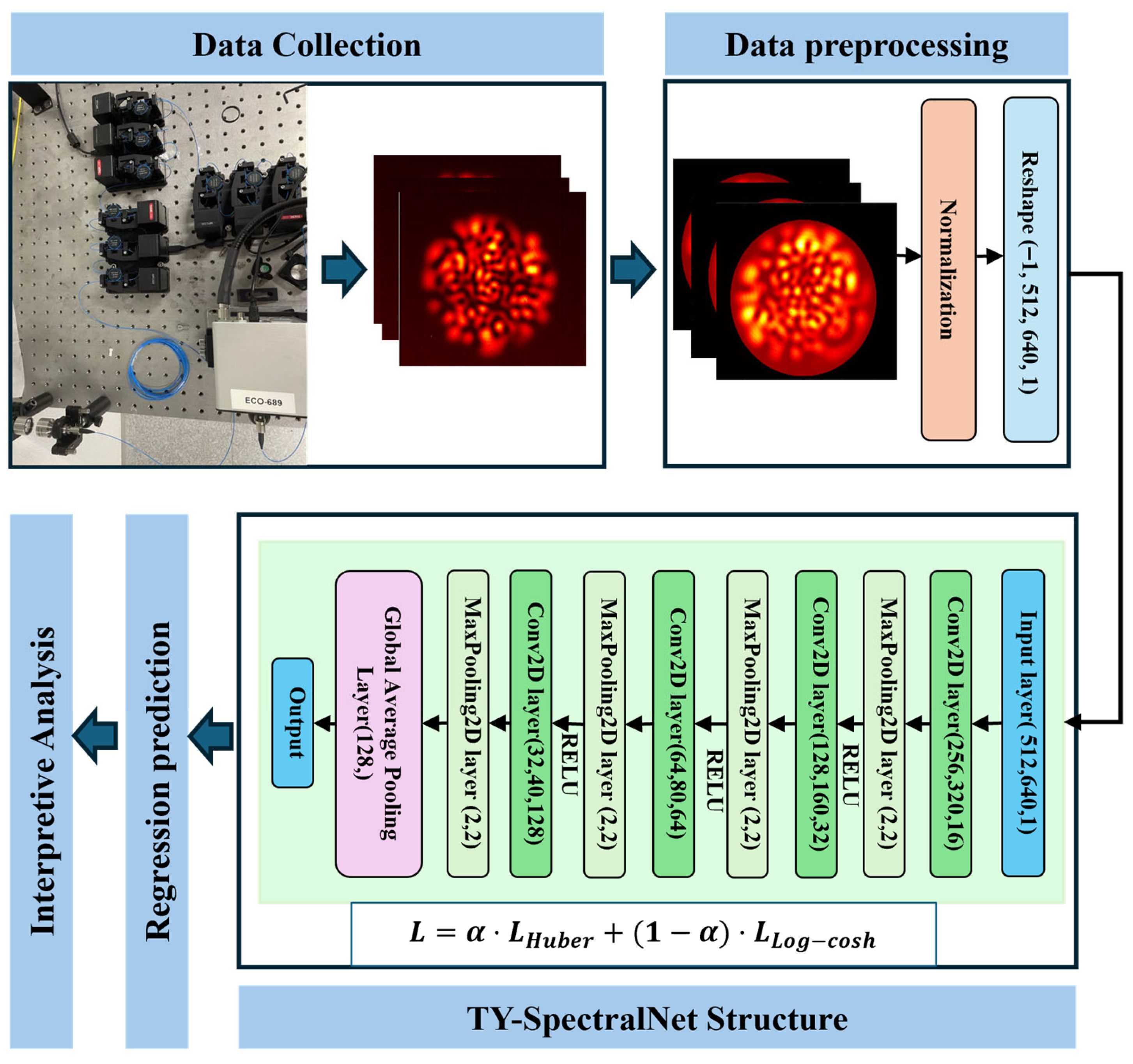
The overall framework of the proposed method is shown in Figure 1 and Figure 2, which consist of the following: data collection, data preprocessing, and TY-SpectralNet regression and interpretive Analysis. Each stage is described in detail below.

3.1. Data Collection

The images in this study were acquired using a Xenics XEVA-1005 near-infrared CCD camera (Made in Belgium 2017) in the Optical Communication and Fiber Sensing Laboratory, Eindhoven University of Technology (ECO Group). A multimode quartz optical fiber with a core radius of 62.5 μm was employed, and the illumination source was a tunable laser with a wavelength tuning accuracy of 0.001 nm. During acquisition, the fiber under test was precisely aligned with the CCD sensor plane to ensure accurate projection of the fiber output facet onto the detector array. A collimation lens was used to adjust the divergence angle, and the fiber end face was carefully aligned along the optical axis to minimize geometric distortion and ensure uniform illumination across the detector surface. The experimental setup is shown in Figure 2, followed the MMF device in previous research [20]. The MMF output was mounted on a translation stage, and multiple optical holders with precision adjustment screws were used to align the optical axis. The acquired raw CCD images had a spatial resolution of 512 × 512 pixels across multiple wavelengths, forming the original dataset used in this study. Under ambient laboratory conditions (24.0–26.0 °C, atmospheric pressure), a total of 1880 images were collected in a single acquisition session. Specifically, five complete spectral sweeps were performed within the wavelength range of 1527.7–1565.3 nm at 0.1 nm intervals. In addition, the recorded images inevitably contain environmental noise, stray light, and minor optical artifacts, which provide a realistic basis for evaluating the robustness and generalizability of the proposed model.

3.2. Data Preprocessing

To enhance the quality of the spectral dataset and prepare it for deep learning, several preprocessing steps were applied. First, background regions outside the interference field were eliminated by detecting the circular boundary of the signal region. All pixels beyond this boundary were set to zero, effectively removing stray light and irrelevant artifacts. Following this, pixel intensities within the valid circular region were normalized to the range $[0,1]$, thereby reducing variations in illumination and improving the numerical stability of network training. Finally, the processed images were reshaped into a four-dimensional tensor of size $(-1,512,640,1)$, where $512\times 640$ corresponds to the spatial resolution of each frame and the last dimension represents the single-channel intensity input. Through this sequence of operations, the raw interference images were transformed into a standardized dataset, which served as the input for the proposed regression model.

3.3. Model Development

3.3.1. Neural Network Architecture

In this study, we designed a lightweight network architecture, as shown in Figure 2. The network takes preprocessed spectral images as input and outputs the corresponding reconstructed spectral intensity. The architecture consists of a series of convolutional and pooling layers, where each convolutional block applies the rectified linear unit (ReLU) activation [21] to introduce nonlinearity, followed by max pooling operations to gradually reduce spatial resolution while retaining essential spectral features. To further improve efficiency, a global average pooling (GAP) layer [22] is employed, compressing the learned feature maps into a compact feature vector. This design reduces the number of trainable parameters, mitigates the risk of overfitting, and enables real-time reconstruction performance. For optimization, the network employs the Adam optimizer [23] with an initial learning rate of 0.001. To ensure stable convergence, network weights are initialized using the He initialization strategy. Training was performed with a mini-batch size of 32 for a maximum of 100 epochs, with early stopping based on validation loss to prevent overfitting. All parameters of TY-SpectralNet are shown in

Table 1. TY-SpectralNet architecture parameters.

Layer Type	Kernel Size	Stride	Output Channels	Output Shape	Activation	Notes
Input	–	–	1	512 × 640 × 1	–	Preprocessed spectral image
Conv Block 1	3 × 3	1	16	512 × 640 × 16	ReLU	Feature extraction
Max Pooling	2 × 2	2	–	256 × 320 × 16	–	Spatial down sampling
Conv Block 2	3 × 3	1	32	256 × 320 × 32	ReLU
Max Pooling	2 × 2	2	–	128 × 160 × 32	–
Conv Block 3	3 × 3	1	64	128 × 160 × 64	ReLU
Max Pooling	2 × 2	2	–	64 × 80 × 64	–
Conv Block 4	3 × 3	1	128	64 × 80 × 128	ReLU
Max Pooling	2 × 2	2	–	32 × 40 × 128	–
Conv Block 5	3 × 3	1	256	32 × 40 × 256	ReLU
GAP (Global Avg Pool)	–	–	–	1 × 1 × 256	–	Feature compression
Dense (Regression)	–	–	1	N × 1	Linear	Output reconstructed spectrum

.

To achieve a balance between accuracy and robustness against outliers, an adaptive hybrid loss function is designed by Huber loss [24,25] and Log-Cosh loss [26]. The Huber loss provides robustness by combining the characteristics of MSE for small residuals and MAE for large residuals, while the Log-Cosh loss introduces smoothness and stabilizes gradient updates. The overall objective function is defined as

$$L=\alpha \cdot L_{Huber}+(1-\alpha )\cdot L_{Log-cosh},$$

(1)

where the Huber loss is given by

$$L_{Huber}=\left\{\begin{array}{c}{\displaystyle \frac{1}{2}}{(y-\widehat{y})}^2\left|y-\widehat{y}\right|\le \delta \\ \delta \left|y-\widehat{y}\right|-{\displaystyle \frac{1}{2}}{\delta }^2\left|y-\widehat{y}\right|>\delta \end{array}\right.,$$

(2)

and the Log-Cosh loss is defined as

$$L_{Log-cosh}={\sum }_i\mathrm{l}\mathrm{o}\mathrm{g}\left(\mathrm{c}\mathrm{o}\mathrm{s}\mathrm{h}\right(\widehat{y_i}-y_i\left)\right),$$

(3)

Here, $\alpha \in [0,1]$ is a weighting coefficient that adaptively balances the contributions of the two loss terms. During the training of TY-SpectralNet, $\alpha$ is dynamically updated to optimize reconstruction performance. The initial value is set to $\alpha =0.5$. A step-based adjustment strategy is employed: if the reconstruction accuracy falls below a threshold ($\tau =0.65$), $\alpha$ is either increased or decreased by $\mathsf{\Delta }\alpha =0.05$ in the subsequent iteration. The training process of α is shown in Algorithm 1. According to the Algorithm 1, a larger α makes the loss behave more like Huber (robust to outliers), while a smaller α makes it closer to Log-Cosh (smoother gradients); δ can be kept fixed or tuned via validation if the outlier scale changes.

Algorithm 1. Training Procedure with Adaptive Loss Weighting

Initialize α = 0.5 Set step size Δα = 0.05 Set accuracy threshold τ = 0.65 Set Huber threshold δ (e.g., δ = 1.0) For each training epoch:         For each mini-batch:                 1. Forward pass → obtain prediction ŷ                 2. Compute residual r = ŷ − y                 3. Compute per-sample Huber δ(r):                               huber(r) = 0.5 * r^2                                    if |r| ≤ δ                                                 = δ*|r| − 0.5*δ^2                        otherwise                       L_Huber = mean(huber(r))                 4. Compute Log-Cosh:                               L_LogCosh = mean( log( cosh(r) ) )                 5. Hybrid loss:                               L = α * L_Huber + (1 − α) * L_LogCosh                 6. Backward pass & update weights (Adam)         End         Evaluate model accuracy A_val on validation set         If A_val < τ:                 # Decide direction:                 # - If more robustness to outliers is needed → increase Huber’s weight                 # - If smoother gradients / stability is needed → increase Log-Cosh’s weight                 # (Example heuristic: if RMSE/MAE is high →α+=Δα; else →α −=Δα)                 If need more robustness:                         α ← α + Δα                 Else:                         α ←α − Δα                 Clip α to [0, 1]

3.3.2. Integrated Gradients Interpret

To enhance the transparency of the proposed network, we employed the IG method [27] after model training to interpret the contribution of input features to reconstructed spectral output. Unlike conventional gradient-based attribution techniques, IG accumulates gradient information along a path between a baseline input and the actual input, thereby mitigating the noise and instability typically associated with single-point gradient estimates. Formally, let F: $R^n\to R$ denote the trained model, where $xϵR^n$ is the input and $x$’ is a baseline input (e.g., a zero image or average background). The attribution assigned by IG to the $i^{th}$ input feature is defined as:

$${IG}_i\left(x\right)=\left(x_i-{x_i}^{\prime }\right)\cdot {\int }_0^1{\displaystyle \frac{\partial F(x^{\prime }+\beta \cdot (x-x^{\prime }\left)\right)}{\partial x_i}}d\beta ,$$

(4)

where the integral is taken along the straight-line path from the baseline $x\mathrm{’}$ to the actual input $x$.

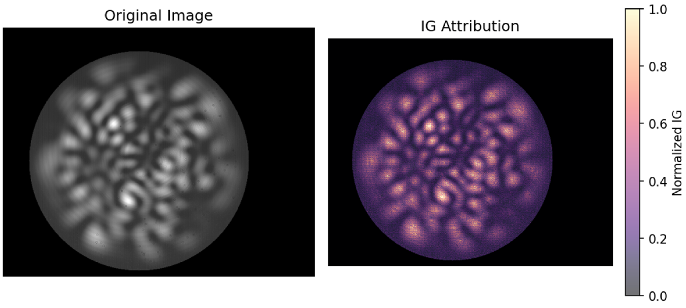
In our study, the CCD interference images were used as inputs, while a zero-image served as the baseline. The resulting IG attribution maps highlighted critical interference patterns and spatial regions that strongly influenced the reconstructed spectral intensities. By establishing a transparent connection between raw spectral images and model predictions, the IG framework not only improves the interpretability of TY-SpectralNet, but also provides valuable physical insights, potentially guiding future sensor calibration and optical system design.

3.4. Experiments Setup

To evaluate the performance of TY-SpectralNet, the collected CCD spectral images were divided into a development set and a validation set. Specifically, 85% of the data were used for model development (including training and hyperparameter tuning), and the remaining 15% were reserved as an independent validation set. In addition, we conducted five-fold cross-validation on the development set to ensure the stability and robustness of the model; during this process, the independent validation set was not used. Two types of reconstruction tasks were performed: (1) single-spectrum wavelength prediction, in which each CCD image corresponded to one spectral distribution, and (2) dual-spectrum wavelength prediction, in which two spectral images of different wavelengths were superimposed in equal proportions to form composite inputs. The proposed models were trained using the development subsets and were subsequently evaluated on the held-out validation sets.

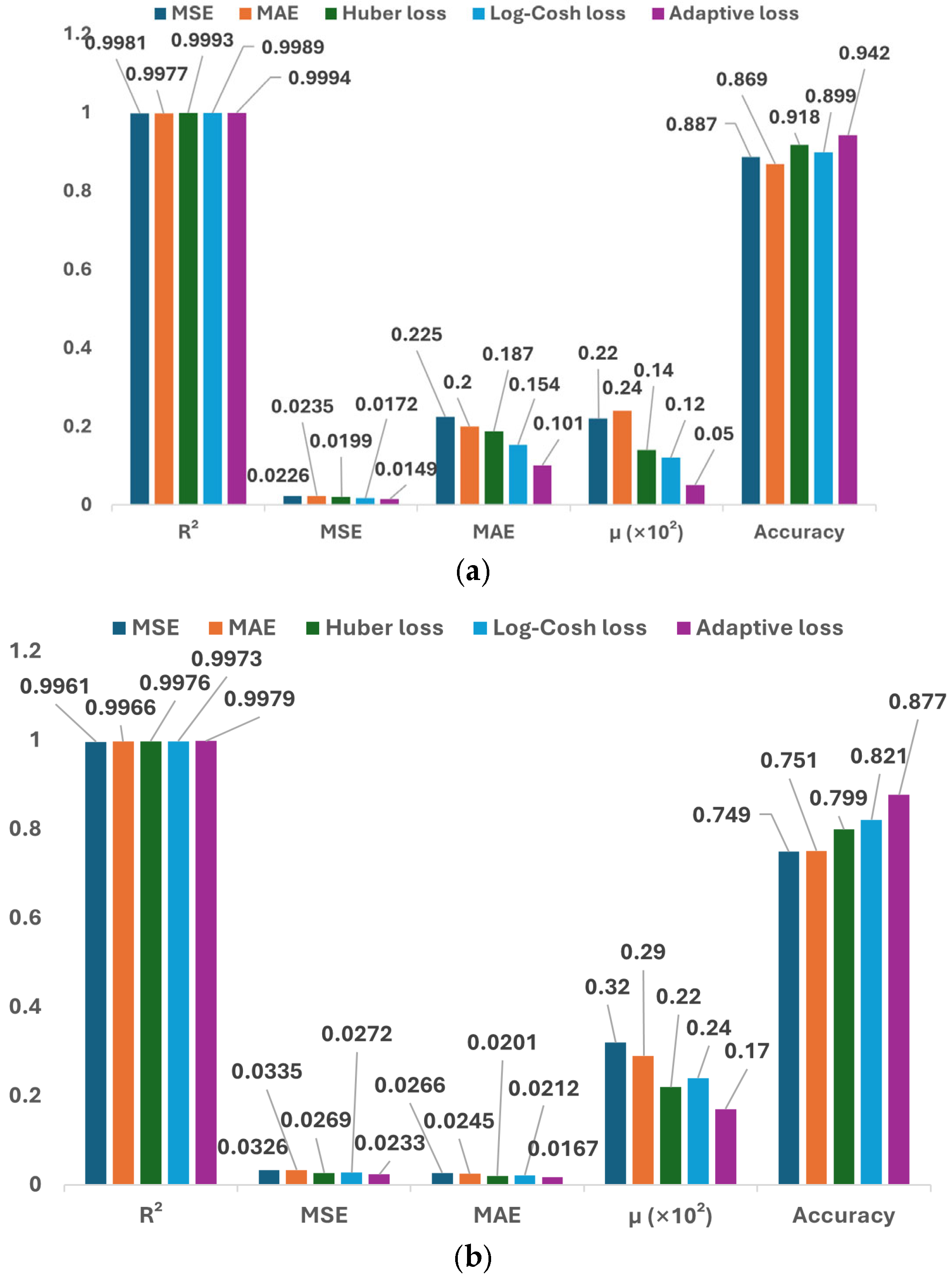
To further investigate the contribution of each component in the proposed adaptive hybrid loss, we conducted an ablation study. Specifically, the full TY-SpectralNet trained with the adaptive loss (Equation (1)) was compared against variants trained with individual loss functions, namely MSE, MAE, Huber loss, and Log-Cosh loss. For interpretability analysis, a zero image was selected as the baseline input, representing the absence of optical interference signals, and the integration path was discretized into m = 50 steps, which provides a balance between computational efficiency and numerical stability. In addition, fine-grained interpretability analyses were performed by examining attribution patterns across different wavelength bands and under varying noise conditions.

To enable parameter optimization, training, and evaluation of models, we chose Python 3.10 as the programming language and TensorFlow 2.13.0 as the deep learning framework. Two NVIDIA RTX A5000 GPUs were used to perform computations. We used the “ReduceLROnPlateau” method [28] to adjust the learning rate during training. The “Adam” optimizer [29] was applied to minimize our class-aware loss and learn the model weights.

3.5. Evaluation and Comparison

The performance of the proposed framework was quantitatively evaluated using regression and classification metrics. For regression tasks, the MSE was adopted to measure the average squared difference between the reconstructed spectral values $\widehat{y_i}$ and the corresponding ground truth $y_i$:

$$MSE={\displaystyle \frac{1}{N}}{\sum }_{i=1}^N{(y_i-\widehat{y_i})}^2,$$

(5)

where $N$ denotes the number of spectral samples.

The coefficient of determination $\left(R^2\right)$ was computed to evaluate the goodness of fit between the predicted and reference spectra:

$$R^2=1-{\displaystyle \frac{{\sum }_{i=1}^N{(y_i-\widehat{y_i})}^2}{{\sum }_{i=1}^N{(y_i-\overline{y})}^2}},$$

(6)

where $\overline{y}$ is the mean of the ground truth values.

To further normalize reconstruction errors across different intensity ranges, the normalized error (μ) was introduced:

$$\mu ={\displaystyle \frac{1}{N}}{\sum }_{i=1}^N{\displaystyle \frac{|y_i-\widehat{y_i}|}{\max \left(y\right)-\mathrm{m}\mathrm{i}\mathrm{n}\left(y\right)}},$$

(7)

For classification-based evaluation, the validation accuracy (ACC) was reported, defined as the proportion of correctly classified spectral categories:

$$ACC={\displaystyle \frac{N_{correct}}{N_{total}}}\times 100\%,$$

(8)

where $N_{correct}$ and $N_{total}$ denote the number of correctly predicted and total samples, respectively.

4. Results

4.1. Single-Spectrum Wavelength Prediction Task

In the single-spectrum wavelength task, each CCD image corresponded to one spectral distribution. As shown in

Table 2. Performance of the TY-SpectralNet on single-spectrum reconstruction.

Model Folds	MSE	R2	μ	ACC (Validation)
Fold 1	0.0123	0.9989	0.0008	90.99%
Fold 2	0.0147	0.9993	0.0006	93.33%
Fold 3	0.0156	0.9994	0.0006	93.63%
Fold 4	0.0127	0.9996	0.0004	96.24%
Fold 5	0.0192	0.9997	0.0003	96.87%
Total (average)	0.0149	0.9994	0.0005	94.21%

, the model consistently achieved low MSE values (average of 0.0149) and high R² values (average of 0.9994) across the five folds. The normalized error μ remained below 0.0010 in most folds, indicating that the predicted spectra closely matched the ground truth within a narrow margin of variation. These results confirm that the proposed method provides accurate and reliable single-spectrum wavelength from CCD interference images. The convergence behavior of the proposed model is shown in Figure 3a. Both the training and validation losses decrease rapidly within the first 200 epochs and then stabilize at a low level. The regression accuracy of the model is shown in Figure 3b, where the predicted spectral values closely align with the ground truth along the diagonal line.

4.2. Dual-Spectrum Wavelength Prediction Task

To further evaluate the capability of TY-SpectralNet in handling more complex spectral information, we conducted experiments on the dual-spectrum wavelength task. The training and validation loss curves are shown in Figure 4a. Both curves show a stable convergence, with validation loss closely following the training loss. A representative reconstruction result is shown in Figure 4b, where the predicted spectra (blue solid line) are compared with the ground truth spectra (red dashed line). The figure shows that peaks are well aligned with the true wavelengths.

Quantitative results are summarized in

Table 3. Performance of the TY-SpectralNet on dual-spectrum reconstruction.

	MSE		R2		μ		ACC (Validation)
	Target 1	Target 2	Target 1	Target 2	Target 1	Target 2	(Average)
Fold 1	0.0251	0.0216	0.9976	0.9991	0.0020	0.0014	88.02%
Fold 2	0.0223	0.0261	0.9982	0.9970	0.0017	0.0021	86.88%
Fold 3	0.0209	0.0251	0.9993	0.9976	0.0011	0.0020	90.01%
Fold 4	0.0212	0.0253	0.9989	0.9942	0.0012	0.0020	87.06%
Fold 5	0.0243	0.0209	0.9981	0.9993	0.0019	0.0011	86.32%
Total (average)	0.0228	0.0238	0.9984	0.9974	0.0016	0.0017	87.66%

. The TY-SpectralNet achieved an average MSE of 0.0228 for Target 1 and 0.0238 for Target 2, with corresponding coefficient of $R^2$ values of 0.9984 and 0.9974. $\mu$ remained at 0.0016 and 0.0017 for the two targets, respectively.

4.3. Ablation Experiments

We further conducted a comparative evaluation of different loss functions, including MSE, MAE, Huber loss, Log-Cosh loss, and the proposed adaptive hybrid loss L, on both the single-spectrum wavelength prediction task and the dual-spectrum wavelength prediction task. The results are summarized in Figure 5. Across both tasks, the adaptive loss consistently achieves the best trade-off between accuracy and robustness, shows superior performance compared with other loss functions.

4.4. Model Explanation Analysis

Figure 6 shows the attribution maps for a representative single-spectrum reconstruction sample. The left panel shows the original CCD image, while the right panel visualizes the IG attributions over the interference region. As observed, the IG heatmap exhibits strong activation along the bright interference fringes. In contrast, peripheral areas with low signal intensity contributed minimally to the predictions.

In the dual-spectrum wavelength prediction task, Figure 7 presents the visualization results for a representative dual-wavelength input. Specifically, Figure 7a shows the raw CCD interference pattern corresponding to the superimposed dual-wavelength signal, while Figure 7b,c display the IG attribution maps for Target 1 and Target 2, respectively. Figure 7d shows the difference map between the two attribution results. The IG attribution maps reveal that the model relies on similar global interference patterns when reconstructing both targets, suggesting that shared spatial modulation features play a key role in spectral localization.

Beyond visualization, we further considered quantitative interpretability experiments on faithfulness, stability, and physics-aware metrics. The results are summarized in Figure 8. Figure 8a shows the Faithfulness Deletion Curves, where progressively removing the top 50% of pixels ranked by IG attribution leads to a pronounced decline in prediction accuracy, with a slope considerably steeper than that of the random deletion baseline. In Figure 8b, the stability metric decreases only slightly as the input noise standard deviation increases, consistently remaining above 0.9 across tested conditions. Figure 8c presents the physics-aware metrics, showing that most top-k IG pixels are concentrated within the 80% encircled energy (EE80) radius, while the centroid shift grows gradually with noise, but remains within only a few pixels.

5. Discussion

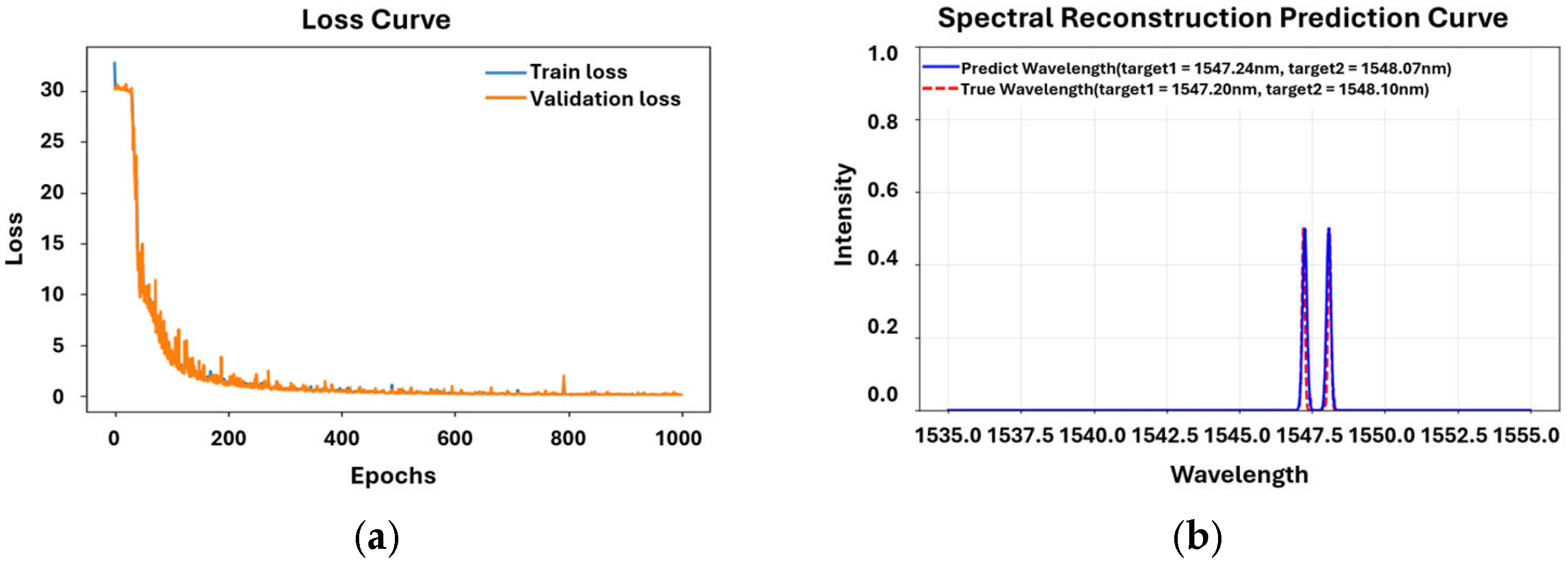
In this study, we applied deep learning with a dynamic adaptive loss function to high-dimensional optical analysis in MMFs and show that a lightweight neural network architecture can achieve high performance in both single- and dual-wavelength prediction tasks. A key contribution of this work lies in the integration of interpretability into the proposed TY-SpectralNet, which enhances both its transparency and practical usability. By employing IG, we were able to clearly identify how different spatial regions of the CCD interference patterns contribute to wavelength prediction.

According to recent surveys on deep learning applied to MMFs spectroscopy, several representative studies have demonstrated the potential of neural networks for wavelength prediction. For example, Yuxuan Xiong et al. [30] introduced a CNN-based WP-Net model in a 2 m MMF, achieving a wavelength precision of 0.045 pm at 1500 nm. Hui Cao et al. [31] employed a 100 m MMF to reach 1 pm resolution at 1500 nm, although their approach was limited to narrowband single-point measurements with a linewidth at the picometer scale. Some works have explored broadband wavelength estimation, such as Hui Cao et al. who achieved 1 nm resolution over a 400–750 nm bandwidth using a 4 cm MMF. More recently, Roopam K. Gupta et al. [32] leveraged a CNN model to provide attometer-scale wavelength precision across a spectral range of 488–976 nm. Despite these advances, to the best of our knowledge, no existing deep learning approach has addressed high-precision prediction specifically in the near-infrared band (1527–1565 nm), which is particularly relevant to optical communication systems. The method proposed in this study not only enables automatic single-wavelength prediction in MMF, but also extends to dual-wavelength prediction under equal-energy conditions. Moreover, the proposed TY-SpectralNet has a computational complexity of 4.68 G FLOPs and an average running time of 5.22 s per inference. While we were unable to identify comparable FLOP or runtime metrics in the exact same domain, we note that representative methods in hyperspectral image reconstruction exhibit substantially higher computational costs. For example, Coupled Nonnegative Matrix Factorization (CNMF, Yokoya et al. [33]) reports an average runtime of ~13 s, HySure [34] requires ~53 s, and TFNet34 [35] involves 5.3 GFLOPs with a runtime of nearly 90 min. These comparisons indicate that TY-SpectralNet achieves a favorable balance between accuracy and efficiency. This capability lays the groundwork for future developments in full-spectrum reconstruction and energy ratio estimation, advancing both the accuracy and versatility of MMF-based spectral sensing.

From a physical perspective, the attribution analysis provides important insight into how the model exploits information embedded in multimode interference. In the single-wavelength case, IG attributions strongly emphasize bright interference fringes, which are physically known to encode wavelength-dependent phase differences. This suggests that the model does not simply memorize training samples, but has learned to extract the same modal features that human experts and optical theory recognize as wavelength carriers. In the dual-wavelength scenario, the attribution maps reveal that the model simultaneously leverages global interference patterns shared by both signals while distinguishing subtle local variations to separate spectral components. This behavior resonates with the physical principle that overlapping modes in MMF generate superimposed interference fringes, where global features correspond to average modal distributions while local perturbations encode fine spectral differences. The quantitative interpretability metrics further support these findings. Faithfulness experiments show that removing the most highly attributed pixels leads to a sharp drop in performance, confirming that the model’s attributions align with causally important regions. Stability analysis demonstrates that attribution maps remain highly consistent under noise perturbations, reflecting the robustness of interference-based wavelength encoding. Physics-aware evaluations reveal that most IG hotspots fall within the 80% encircled energy (EE80) radius, directly linking the model’s learned focus to physically meaningful energy distributions. Moreover, the centroid shift remains limited to pixel-scale deviations even under high noise, which is consistent with the physical stability of fiber mode centroids against perturbations. This interpretability not only enhances confidence in the model’s predictions, but also provides a feedback loop for refining experimental design, such as optimizing CCD alignment or selecting regions of interest for data acquisition.

There are several limitations in this study. First, the experimental data acquisition process is inevitably subject to noise. The dominant source of noise in image acquisition originates from the CCD camera, which primarily consists of readout noise, dark current noise, photon noise, and fixed pattern noise. Among these, dark current noise can be mitigated through background subtraction, while photon noise and readout noise are commonly reduced via normalization procedures. Fixed pattern noise, however, requires camera-specific correction techniques, such as flat-field correction. In addition to these intrinsic noise sources, extrinsic factors including stray light and experimental artifacts can further compromise image quality. Due to current laboratory constraints, only background subtraction and normalization are employed during data preprocessing. Consequently, the CCD-acquired images still retain a certain degree of residual noise. Future work will aim to improve data quality by incorporating advanced denoising strategies and exploring adaptive noise-robust learning techniques. Second, the current optical platform is constructed on a multimode fiber polarization control module in conjunction with a multimode fiber mode excitation unit. This configuration employs a fixed angular reference and achieves an optimized excitation state of multimode fiber modes through regulation by the polarization controller. While this arrangement enables stable mode excitation and ensures experimental repeatability, it inherently constrains the variability of the interference patterns that can be captured. Considering that the wide wavelength span and dense sampling interval already result in a large dataset, the polarization angle was not dynamically varied in this study. In future work, we plan to relax this constraint and explore dynamic angular variation, which may introduce additional degrees of freedom and enable more comprehensive and automated wavelength prediction across higher-dimensional parameter spaces. Third, the framework developed in this research is restricted to single-spectrum and equal-energy dual-spectrum reconstruction tasks. While excellent performance was demonstrated in these relatively simple cases, its applicability to more complex scenarios—such as multi-spectrum or multi-energy spectral reconstruction—remains to be explored. Extending the framework to these tasks will require addressing more diverse spectral compositions and nonlinear interactions between multiple wavelengths or energy levels. We posit that deep learning techniques hold substantial potential for enabling full-spectrum analysis. Established architectures such as ResNet [36] and Transformer [37] have demonstrated strong representational capacity, providing a foundation for more advanced modeling. Beyond these, deeper architectures incorporating paradigms such as contrastive learning [38], transfer learning [39], and twin-network learning [40] may further facilitate comprehensive spectral scanning while enhancing model adaptability and generalization. In terms of experimental platforms and data acquisition, future efforts will focus on employing platforms that provide greater flexibility and controllability, alongside data collection strategies that yield higher signal-to-noise ratios.

6. Conclusions

In this study, we proposed a lightweight deep learning framework, TY-SpectralNet, which integrates an adaptive dynamic loss function for single- and dual-spectral wavelength prediction in MMFs. Experimental results achieve MSE consistently below 0.024 and R² values above 0.99. Through interpretability analysis, we further showed that the network attends to physically meaningful interference fringes in single-spectral tasks and adaptively differentiates local features in dual-spectral scenarios. Moreover, TY-SpectralNet achieves low computational overhead, with only 4.68 G FLOPs and an average running time of 5.22 s per prediction. Future work will extend TY-SpectralNet to more complex tasks, including multi-wavelength and multi-energy reconstruction, thereby advancing its applicability in high-dimensional spectral sensing and optical communication systems.