Neural-Network-Based Adaptive MPC Path Tracking Control for 4WID Vehicles Using Phase Plane Analysis

Abstract

To improve the adaptability of 4WID electric vehicles under various operating conditions, this study introduces a model predictive control approach utilizing a neural network for adaptive weight parameter prediction, which integrates four-wheel steering and longitudinal driving force control. To address the difficulty in adjusting the MPC weight parameters, the neural network undergoes offline training, and the Snake Optimization method is used to iteratively optimize the controller parameters under diverse driving conditions. To further enhance vehicle stability, the real-time stability state of the vehicle is assessed using the $\beta -\dot{\beta }$ phase plane method. The influence of vehicle speed and road adhesion on the instability boundary of the phase plane is comprehensively considered to design a stability controller based on different instability degree zones. This includes an integral sliding mode controller that accounts for both vehicle tracking capability and stability, as well as a PID controller, which calculates the additional yaw moment based on the degree of instability. Finally, an optimal distribution control algorithm coordinates the longitudinal driving torque and direct yaw moment while also considering the vehicle’s understeering characteristics in determining the torque distribution for each wheel. The simulation results show that under various operating conditions, the proposed control strategy achieves smaller tracking errors and more concentrated phase trajectories compared to traditional controllers, thereby improving path tracking precision, vehicle stability, and adaptability to varying conditions.

1. Introduction

As a key component of intelligent transportation systems, advancements in autonomous mobility have garnered significant attention, especially in academia and industry [1,2]. Path tracking control is a crucial technology for autonomous vehicles, aiming to reduce the discrepancy between the actual trajectory and the desired trajectory by considering the vehicle’s real-time dynamics [3]. However, when the vehicle is traveling at a rapid pace or operating on a slippery road surface, it is prone to losing stability and deviating from the target trajectory [4]. Therefore, designing a path tracking control method that maintains high accuracy and strong robustness under complex driving conditions is of great significance for enhancing the safety and reliability of autonomous driving systems.

Existing path tracking techniques mainly include PID control, Pure Pursuit control [5], backstepping control [6], fuzzy logic control [7], LQR control [8], sliding mode approach [9], and Model Predictive Control [10,11]. Among these, Model Predictive Control has been extensively utilized in path tracking applications owing to its predictive nature and distinct advantages in handling nonlinear dynamics and multi-constraint problems [12]. However, it still faces some challenges. Many researchers have proposed improvements such as optimizing controller parameters, enhancing model accuracy [13], and adding constraints [14]. Wu et al. [15], by analyzing the impact of the prediction horizon and weighting factors on trajectory accuracy and vehicle yaw stability, plotted the corresponding relationships as three one-dimensional lookup tables, achieving adaptive adjustment of the controller parameters. Yang and Liu [16] proposed a rule-based adaptive prediction horizon MPC for lateral tracking control and fuzzy PID for forward motion control, which is adapted to changes in vehicle speed. Wang et al. [17] utilized a fuzzy logic-based approach to dynamically tune the lateral displacement weight coefficient in the MPC trajectory following controller, considering both the average deviation and its rate of change. Yang et al. [18] designed a trajectory tracking control strategy based on a T–S fuzzy variable-weight MPC controller. The lateral error and heading error are used as fuzzy inputs, while the weighting factors for lateral error, yaw rate error, velocity error, and control increment are treated as outputs. By analyzing the relationship between the outputs and the vehicle states, fuzzy rules are formulated to achieve adaptive adjustment of the controller parameters. Xue and Zheng [19] developed an adaptive model predictive controller with flexible sampling and prediction intervals, incorporating a rounding function and a contraction factor, where the adaptation is guided by the average curvature’s second-order derivative. Although the aforementioned methods have improved the adaptability of path tracking controllers to complex driving environments to some extent, most of them rely on manually designed lookup tables or fuzzy logic rules. The parameter tuning process heavily depends on empirical knowledge or prior experience and lacks theoretical optimization foundations, making the controller performance is susceptible to subjective factors. In addition, these methods often suffer from insufficient tracking accuracy and degraded stability under extreme conditions such as high speeds, sharp turns, or low-adhesion road surfaces, making it difficult to meet the robustness and safety requirements of autonomous vehicles in complex driving scenarios. Wang et al. [20] developed a path-tracking strategy utilizing model predictive control with an adaptive prediction horizon, optimized using particle swarm optimization. The method theoretically possesses strong global optimization capabilities and can adapt to various road conditions and vehicle states. However, as an online optimization algorithm, particle swarm optimization typically requires a large number of iterations and multiple objective function evaluations, placing high demands on system computational resources and response time, which significantly increases the online computational burden of the controller. Moreover, due to the potential sensitivity to initial values, the stability and convergence of the optimization results cannot be reliably guaranteed under complex driving conditions.

The lateral controllers in the aforementioned studies only control the front-wheel turning angle. Advancements in autonomous driving technology have enabled the development of vehicles with independently controlled steering and drive systems, providing a platform for advanced control strategies like Active Front/Rear-Wheel Steering (AFS/ARS) and Direct Yaw Moment Control (DYC) [21,22].The direct yaw moment control strategy primarily adopts a traditional layered framework, where the higher-level controller obtains the wheel angles and generalized forces, while the lower level controller distributes the generalized forces to the four wheels [23]. Ren et al. [24] introduced a unified control approach that combines longitudinal force with front-axle turning angle MPC to fully leverage the advantages of the MPC controller in solving multi-constraint problems. Numerous studies have employed the phase plane analysis to examine the dynamic behavior of vehicles, aiming to resolve the coupling issue between vehicle tracking performance and stability [25]. Liu and Dai [26] proposed a coordinated control approach for AFS and DYC, where the instability degree obtained from the $\beta -\dot{\beta }$ phase plane analysis is used as the controller’s intervention condition. A switching function is designed based on the edge density function of a normal distribution to smoothly transition between the weight coefficients of the two controllers. Zhu et al. [27] employed an adaptive fuzzy controller and the phase plane method to regulate the quantization and scale factors for calculating the required additional yaw moment. Wang and Song [28] introduced an error penalty into the optimal distribution control objective function and modified the weight matrix using the vehicle’s steady-state coefficients obtained through $\beta -\dot{\beta }$ phase plane analysis, optimizing the torque distribution across the wheels during vehicle operation. This method considers the vehicle’s dynamic response during driving to optimize the conditional constraints in the torque distribution strategy, thereby enhancing control performance under specific stability requirements. However, it does not incorporate the longitudinal dynamic response into the control framework, lacking coordinated control over the coupling between vehicle power performance and stability. In real-world scenarios, the vehicle’s longitudinal driving capability and lateral stability are often mutually constrained. Ignoring such coordination under extreme conditions may lead to vehicle instability and compromise driving safety.

Based on the above analysis and discussion, this paper proposes an adaptive path tracking control algorithm for distributed drive electric vehicles, aiming to address several critical issues identified in relevant studies from 2023 to 2025, as summarized in

Table 1. Literature review and analysis.

Ref.	Approach	Limitations
Wu [15]	By analyzing the impact of the prediction horizon and weighting factors on trajectory accuracy and vehicle yaw stability, corresponding relationships were plotted as three one-dimensional lookup tables to achieve adaptive adjustment of controller parameters.	Lookup tables can only express the relationship between individual control parameters and single factors, such as tracking accuracy or yaw stability. However, controller parameters are often influenced by the nonlinear coupling of multiple variables simultaneously. This may lead to decreased controller accuracy or oversimplification of system behavior.
Wang [20]	A path tracking strategy utilizing model predictive control with an adaptive prediction horizon was developed. This strategy was optimized using particle swarm optimization.	The particle swarm algorithm requires evaluating multiple particles and performing several updates in each iteration. If Particle Swarm Optimization (PSO) is used is used for parameter optimization in the online control phase, it will result in significant computational delays, making it difficult to meet real-time requirements.
Wang [28]	A comprehensive controller for wheel steering angles and additional yaw moment was developed, where real-time adjustment of the control matrix weights was achieved through the vehicle’s steady-state parameters. The optimal torque distribution for each tire was ultimately achieved by minimizing the tire load ratio.	The adjustment of control weights, guided by vehicle steady-state parameters, serves as the optimization goal for torque distribution at the execution layer. However, the control strategy does not assign fixed weights to lateral and heading errors in the path tracking controller. In different speed or road conditions, fixed error weights cannot balance the conflict between path accuracy and vehicle stability.

. First, existing adaptive MPC approaches generally rely on either predefined rules or fully depend on optimization algorithms. The former suffers from strong subjectivity in controller design, while the latter incurs a high online computational burden, limiting their applicability under complex driving conditions. Second, many existing methods fail to adequately consider the vehicle’s adaptability to varying environments, making it difficult for the system to handle highly dynamic and uncertain driving scenarios. Furthermore, under dynamic driving conditions, there exists a significant coupling between path tracking performance and vehicle stability. Current control strategies lack effective coordination mechanisms to address this coupling and often neglect the influence of longitudinal driving performance on vehicle stability, which ultimately compromises overall control performance. The main contributions of this paper are as follows:

(1)

The Back Propagation (BP) neural network is utilized to model the intricate non-linear correlation between the MPC weight coefficients and trajectory tracking precision along with dynamic stability, reducing the reliance on manually designed lookup tables or fuzzy logic rules and minimizing the influence of subjective factors. To optimize the weights and biases of the neural network during backpropagation, the Snake Optimization method is employed for iterative tuning of neural network parameters. The neural network model is trained offline using extensive simulation data, and a fitness criterion is formulated by incorporating both trajectory accuracy and stability to reduce online computation costs. The Snake Optimization algorithm is employed to optimize the MPC weight parameters under different driving conditions.

(2)

To overcome the coupling issue of vehicle tracking capability and stability, a stability control approach utilizing the phase plane method is developed. The dynamic state of the vehicle is analyzed in real-time using the phase plane, and different instability degree-based zone controllers are designed. To ensure smooth switching between controllers, a joint control domain is introduced.

(3)

Addressing the overlooked impact of the vehicle’s longitudinal power performance on stability in the aforementioned studies, this paper ensures that dynamic performance and stability requirements are met by coordinating the longitudinal driving torque and additional yaw moment based on the instability degree and road friction coefficient. The optimal distribution algorithm is designed to determine the driving torques for each wheel, considering the vehicle’s understeer characteristics.

2. Materials and Methods

This paper develops an integrated path tracking controller based on Model Predictive Control (MPC) for four-wheel independent drive (4WID) vehicles. The control system is based on a three-DOF vehicle dynamics model, which considers the longitudinal, lateral, and yaw motions of the vehicle. The MPC path tracking controller serves as the core module. To fully exploit the advantages of MPC in handling multi-constraint problems, this study selects the front and rear wheel steering angles and the longitudinal driving forces as control variables. The performance of the controller depends on the selection of the weighting matrices Q and R. Improper weighting may lead to reduced tracking accuracy or compromised vehicle stability. The reference model calculates the ideal sideslip angle and yaw rate of the vehicle’s center of mass, which serve as target inputs for the stability control module under varying road conditions.

2.1. Vehicle Model and Ideal Reference Model

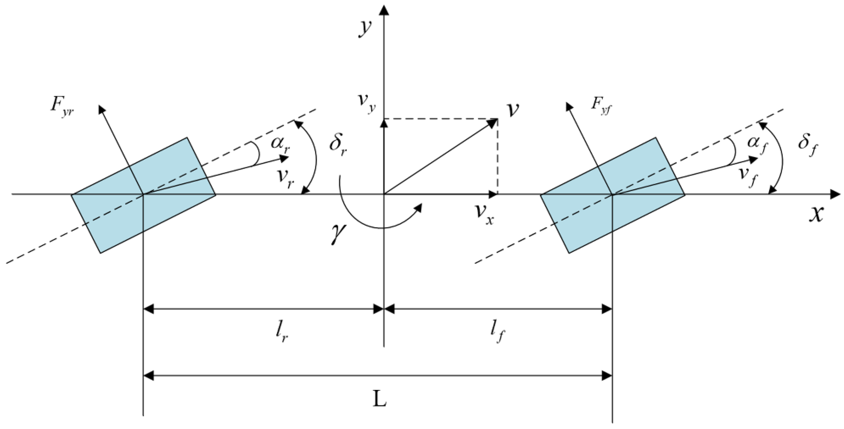
In this study, a three-DOF dynamic equation models the vehicle’s motion characteristics during path tracking. The analysis assumes a small front-wheel steering angle and a constant longitudinal velocity along the x-axis. The model ignores the differences in steering angles between the inner and outer wheels (Ackermann steering geometry), as well as the effects of air resistance and suspension. The corresponding bicycle model is depicted in Figure 1. The lateral and forward movement of the vehicle, along with its yaw dynamics, are captured by Equation (1).

$$\left\{\begin{array}{l}{F}_y=\mathrm{m}({\dot{v}}_y+\gamma v_x)=F_{yf}+F_{yr}\\ F_x=\mathrm{m}({\dot{v}}_x-\gamma v_y)=F_{xf}+F_{xr}\\ I_z\dot{\gamma }=l_f{F}_{yf}-l_r{F}_{yr}\end{array}\right.$$

(1)

In the equation, $m$ represents the vehicle’s total mass. $v_x$ and $v_y$ denote its forward and lateral velocities, respectively. The yaw angular velocity is denoted by $\gamma$. $F_{xf}$, $F_{xr}$, $F_{yf}$ and $F_{yr}$ correspond to the longitudinal and side forces acting on the front-axle and rear-axle tires. $I_Z$ represents the moment of inertia; $l_f$ and $l_r$ indicate the distances from the center of mass to the front-axle and rear-axle. It should be noted that the three-DOF bicycle model used in this study offers a simplified representation of vehicle dynamics under medium- to high-speed driving conditions. Its accuracy decreases at low speeds and large steering angles, such as during parking maneuvers. Therefore, this study focuses on medium- to high-speed scenarios. Future work will extend the model to address low-speed and large steering angle conditions. When the tires function within the linear range, the side force is given by Equation (2).

$$\left\{\begin{array}{l}{F}_{yf}=k_1{\alpha }_f=k_1({\displaystyle \frac{v_y+l_f\gamma }{v_x}}-{\delta }_f)\\ F_{yr}=k_2{\alpha }_r=k_2({\displaystyle \frac{v_y-l_r\gamma }{v_x}}-{\delta }_r)\end{array}\right.$$

(2)

In the equation, $k_1$ and $k_2$ denote the equivalent cornering rigidity of the front-axle and rear-axle. The slip angles of the front-axle and rear-axle are denoted by ${\alpha }_f$ and ${\alpha }_r$, while ${\delta }_f$ and ${\delta }_r$ correspond to their respective steering angles.

In the control framework adopted in this study, the effects of the suspension system and aerodynamic forces are neglected, and parameters such as tire cornering stiffness are simplified as constant values. This modeling approach has been widely adopted in numerous recent studies on lateral control, particularly under typical conditions such as medium- to high-speed driving and lane-keeping scenarios, where it shows strong applicability. When the tire operates within a small slip angle range (typically less than 6°), the variation in cornering stiffness is minimal, making it a reasonable simplification to treat it as a constant [29]. The cornering stiffness parameters were calibrated experimentally at 90 km/h, and have shown effective control performance across a wide range of medium- to high-speed driving conditions. However, it is acknowledged that under extreme dynamic scenarios involving large slip angles, this simplification may not fully capture the actual vehicle dynamics. In future work, we plan to incorporate online parameter estimation methods, as well as suspension and aerodynamic modeling, to improve model adaptability and robustness.

The vehicle’s total mass and inertia properties, along with the front and rear axle cornering stiffness coefficients, were derived from CarSim 2020.0, a validated commercial vehicle dynamics simulation platform. These parameters correspond to a C-Class Hatchback passenger car model embedded in CarSim’s database, which has been extensively adopted in both academic research and engineering practice due to its realism and representative nature.

The tire’s rotational dynamics are expressed as:

$$I_w\dot{\omega }=T-R_{w}F$$

(3)

where $I_w$ is the tire’s rotational inertia, $\omega$ is the angular velocity of the tire. $R_w$ is the tire radius, $F$ and $T$ respectively represent the longitudinal force and driving torque of the tire. Equation (1) can be derived and expressed as a differential equation in Equation (4).

$$\left\{\begin{array}{l}{\dot{v}}_x={\displaystyle \frac{m{v}_y{R}_w^2}{m{R}_w^2+I_w}}\gamma +{\displaystyle \frac{R_w}{m{R}_w^2+I_w}}T\\ {\dot{v}}_y={\displaystyle \frac{k_1+k_2}{m{v}_x}}{v}_y+({\displaystyle \frac{l_f{k}_1-l_r{k}_2}{m{v}_x}}-v_x)\gamma -{\displaystyle \frac{k_1}{m}}{\delta }_f-{\displaystyle \frac{k_2}{m}}{\delta }_r\\ \dot{\gamma }={\displaystyle \frac{l_f{k}_1-l_r{k}_2}{I_z{v}_x}}{v}_y+{\displaystyle \frac{{l_f}^2{k}_1+{l_r}^2{k}_2}{I_z{v}_x}}\gamma -{\displaystyle \frac{l_f{k}_1}{I_z}}{\delta }_f+{\displaystyle \frac{l_r{k}_2}{I_z}}{\delta }_r\end{array}\right.$$

(4)

Taking road adhesion limitations into account, the maximum allowable angular velocity and body slip angle are derived from Equation (5).

$$\left\{\begin{array}{l}\left|{\gamma }_{\max }\right|={\displaystyle \frac{0.85\mu g}{v_x}}\\ \left|{\beta }_{\max }\right|=0.85\mu g({\displaystyle \frac{l_r}{v_x^2}}+{\displaystyle \frac{m{l}_f}{k_{r}L}})\end{array}\right.$$

(5)

The ideal reference model characterizes the vehicle’s lateral dynamics under steady-state conditions. When the vehicle maintains a steady state, $\dot{\beta }=0$ and $\dot{\gamma }=0$. The required vehicle’s ideal angular velocity and body slip angle for the system are computed as shown in Equation (6).

$$\left\{\begin{array}{l}{\gamma }_d=\min \left\{\left|{\displaystyle \frac{v_x}{L(1+K{v}_x^2)}}{\delta }_f\right|,|{\gamma }_{\max }|\right\}\mathrm{sgn}({\delta }_f)\\ {\beta }_d=\min \left\{\left|{\displaystyle \frac{l_r/L+m{l}_f{v}_x^2/(k_r{L}^2)}{1+K{v}_x^2}}{\delta }_f\right|,|{\beta }_{\max }|\right\}\mathrm{sgn}({\delta }_f)\end{array}\right.$$

(6)

where $\mu$ denotes the road friction coefficient, and $g$ is the gravitational acceleration. The parameters $L$ and $K$ correspond to the wheelbase and vehicle stability factor, respectively. Additionally, ${\gamma }_d$ signifies the ideal yaw rate, and ${\beta }_d$ refers to the ideal center of mass slip angle.

2.2. MPC Path Tracking Model

During path tracking control, the following relationship exists:

$$\left\{\begin{array}{l}\dot{X}=v_x-v_y\phi \\ \dot{Y}=v_x\phi +v_y\\ \dot{\phi }=\gamma \end{array}\right.$$

(7)

In the equation, $\phi$ represents the vehicle’s heading angle, $X$ and $Y$ denote its forward and lateral positions in the global coordinate system.

Based on Equation (4), the system can be transformed into state-space representation. The state variables are taken as $x={\left[X,Y,\phi ,v_x,v_y,\gamma \right]}^T$, the control parameters as $u={\left[{\delta }_f,{\delta }_r,T\right]}^T$, and the output variables as: $y={\left[X,Y,\phi \right]}^T$. The resulting state-space equation is presented in Equation (8).

$$\left\{\begin{array}{l}\dot{x}=Ax+Bu\\ y=Cx+Du\end{array}\right.$$

(8)

where:

$$A=\left[\begin{array}{cccccc}0& 0& -v_y& 1& 0& 0\\ 0& 0& v_x& 0& 1& 0\\ 0& 0& 0& 0& 0& 1\\ 0& 0& 0& 0& 0& {\displaystyle \frac{m{v}_y{R}_w^2}{m{R}_w^2+I_w}}\\ 0& 0& 0& 0& {\displaystyle \frac{k_1+k_2}{m{v}_x}}& {\displaystyle \frac{(l_f{k}_1-l_r{k}_2)}{m{v}_x}}-v_x\\ 0& 0& 0& 0& {\displaystyle \frac{(l_f{k}_1-l_r{k}_2)}{I_z{v}_x}}& {\displaystyle \frac{({l_f}^2{k}_1+{l_r}^2{k}_2)}{I_z{v}_x}}\end{array}\right], B=\left[\begin{array}{ccc}0& 0& 0\\ 0& 0& 0\\ 0& 0& 0\\ 0& 0& {\displaystyle \frac{R_w}{m{R}_w^2+I_w}}\\ -{\displaystyle \frac{k_1}{m}}& -{\displaystyle \frac{k_2}{m}}& 0\\ -{\displaystyle \frac{l_f{k}_1}{I_z}}& {\displaystyle \frac{l_r{k}_2}{I_z}}& 0\end{array}\right], C={\left[\begin{array}{ccc}0& 0& 1\\ 0& 1& 0\\ 1& 0& 0\\ 0& 0& 0\\ 0& 0& 0\\ 0& 0& 0\end{array}\right]}^T, D=\left[\begin{array}{c}0\\ 0\\ 0\end{array}\right]$$

Assuming the current state is ${\dot{x}}_0=f(x_0,u_0)$, performing the Taylor series expansion while retaining only the first-order terms yields:

$$\dot{x}=f(x_0,u_0)+A_t(x-x_0)+B_t(u-u_0)$$

(9)

By subtracting Equation (9) from the current state point, we obtain:

$$\dot{\tilde{x}}=A_t(x-x_0)+B_t(u-u_0)$$

(10)

Applying the first-order difference approximation, Equation (10) is discretized using a fixed sampling interval $T_s=0.01$, as shown in Equation (11).

$$\left\{\begin{array}{l}{\tilde{x}}_{k+1}=A_d{\tilde{x}}_k+B_d{\tilde{u}}_k\\ y_k=C_d{\tilde{x}}_k\end{array}\right.$$

(11)

In the equation, $A_d=A_t{T}_s+I_{Nx}$, $B_d=B_t{T}_s$ and $C_d=I_{Nx}$. In order to limit the control inputs, the state and control variables are augmented into a new set of state variables, denoted as ${\xi }_k=\left[\begin{array}{l}{\tilde{x}}_k\\ {\tilde{u}}_{k-1}\end{array}\right]$, and the variation in control inputs at each iteration relative to the preceding one is represented by $\Delta {\tilde{u}}_k$, which gives Equation (12).

$$\left\{\begin{array}{l}{\zeta }_{k+1}=A_1{\xi }_k+B_1\Delta {\tilde{u}}_k\\ {\eta }_k=C_1{\xi }_k\end{array}\right.$$

(12)

where: $A_1=\left[\begin{array}{cc}{A}_d& B_d\\ 0_{Nu\times Nx}& I_{Nu\times Nu}\end{array}\right]$, $B_1=\left[\begin{array}{l}{B}_d\\ I_{Nu\times Nu}\end{array}\right]$, $C_1={\left[\begin{array}{l}{C}_d\\ 0_{Nx\times Nu}\end{array}\right]}^T$. $N_x$ represents the number of state variables. $N_u$ denotes the number of control inputs. Let $k$ denote the current time step. To predict the states and outputs for the next $N_p$ steps, the control input is represented as Equation (13).

$$\Delta U={[\Delta \tilde{u}(k),\Delta \tilde{u}(k+1),\dots ,\Delta \tilde{u}(k+Nc-1)]}^T$$

(13)

where: $\Delta \tilde{u}(i)={\left[\Delta {\delta }_f(i),\Delta {\delta }_r(i),\Delta T(i)\right]}^T,i=k\dots k+Nc-1$. From the above equation, the controller predicts the output $Y$ over the next $N_p$ steps as illustrated in Equation (14).

$$Y=\Psi {\zeta }_k+\Theta \Delta U$$

(14)

where:

$$Y=\left[\begin{array}{l}{\eta }_{k+1}\\ {\eta }_{k+2}\\ \dots \\ {\eta }_{k+Nc}\\ \dots \\ {\eta }_{k+Np}\end{array}\right];\Psi =\left[\begin{array}{l}{C}_1{A}_1\\ C_1{A}_1^2\\ \dots \\ C_1{A}_1^{Nc}\\ \dots \\ C_1{A}_1^{Np}\end{array}\right];\Theta =\left[\begin{array}{cccc}{\mathrm{C}}_1{\mathrm{B}}_1& 0& 0& 0\\ {\mathrm{C}}_1{\mathrm{A}}_1{\mathrm{B}}_1& {\mathrm{C}}_1{\mathrm{B}}_1& 0& 0\\ ⋮& ⋮& \ddots & ⋮\\ {\mathrm{C}}_1{\mathrm{A}}_1^{Nc}{\mathrm{B}}_1& {\mathrm{C}}_1{\mathrm{A}}_1^{Nc-1}{\mathrm{B}}_1& \dots & {\mathrm{C}}_1{\mathrm{A}}_1{\mathrm{B}}_1\\ ⋮& ⋮& \ddots & ⋮\\ {\mathrm{C}}_1{\mathrm{A}}_1^{Np-1}{\mathrm{B}}_1& {\mathrm{C}}_1{\mathrm{A}}_1^{Np-2}{\mathrm{B}}_1& \dots & {\mathrm{C}}_1{\mathrm{A}}_1^{Np-Nc-1}{\mathrm{B}}_1\end{array}\right]$$

To ensure smoothness and stability in the tracking process, the optimization objective is to minimize state deviations and control efforts. This objective is formulated as a quadratic programming problem, as shown in Equation (15).

$$J={(Y-Y_{ref})}^T\mathrm{Q}(Y-Y_{ref})+\Delta {\mathrm{U}}^{T}R\Delta \mathrm{U}+\rho {\epsilon }^2$$

(15)

where: $Q_i=\left[\begin{array}{cc}{q}_1& 0\\ 0& q_2\end{array}\right]$, $R_i=diag(r,r,r)$, $i=1,2,3\dots Np$. $Q_i$ and $R_i$ are the prediction and control matrices for the MPC, respectively. While $q_1$, $q_2$ and $r$ represent the weights for lateral deviation, yaw rate error, and control input variation, respectively. Model Predictive Control needs to solve the optimal control sequence over the prediction horizon while satisfying the objective function and various constraints. The constraints on the four-wheel steering angles, as well as the longitudinal driving force and its rate of change, are expressed as shown in Equation (16).

$$\left\{\begin{array}{l}{\tilde{u}}_{\min }\le \tilde{u}(t+k)\le {\tilde{u}}_{\max },k=0,1,\dots ,N_C-1\\ \Delta {\tilde{u}}_{\min }\le \Delta \tilde{u}(t+k)\le \Delta {\tilde{u}}_{\max },k=0,1,\dots ,N_C-1\end{array}\right.$$

(16)

Considering the limitations of the steering and drive motors, the front wheel steering angle is constrained within the range of [−0.44, 0.44] radians, with a rate limit of [−0.02, 0.02] radians. The rear wheel steering angle is constrained within [−0.44, 0.44] radians, with a rate limit of [−0.005, 0.005] radians. The longitudinal driving torque is constrained to [−600, 600] Nm, with a rate limit of [−50, 50] Nm. These constraints are based on the technical specifications of typical wheel-side motors and steering actuators, and are compatible with the discretization interval of the MPC used in this study [30]. By solving the constrained quadratic optimization problem, the optimal front and rear steering angles and longitudinal driving torque can be obtained. Only the first element of the optimal control sequence is applied at each sampling instant, and the optimization process is repeated at every time step.

2.3. Trajectory Tracking Control System Design for 4WID Vehicles

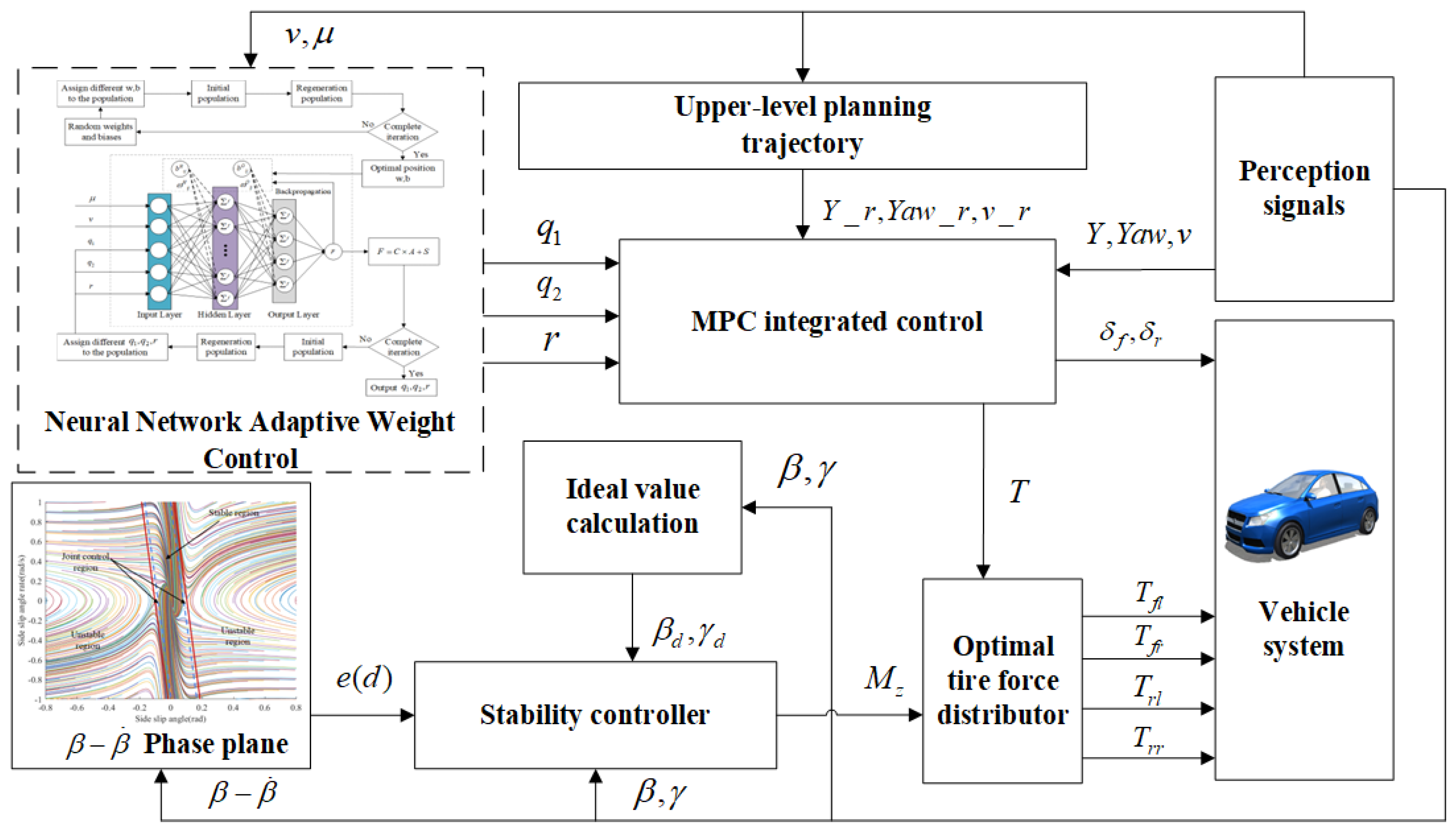
Figure 2 illustrates the framework of the trajectory tracking strategy for a distributed drive vehicle. The planning layer provides road information and vehicle state parameters as inputs to the MPC. Heidfeld et al. [31] use the Unscented Kalman Filter (UKF) method, combining a nonlinear double-track model with a brush tire model, to achieve real-time estimation of vehicle state parameters including vehicle speed, yaw rate, and road friction coefficient. This approach improves the accuracy and robustness of the vehicle system control. Li et al. [32] propose a method for estimating the vehicle’s center of mass side-slip angle based on the non-linear Dugoff tire model and the non-singular terminal sliding mode observer (NS-TSMO). This method improves the accuracy of side-slip angle estimation for vehicles driving under varying road adhesion conditions. The signal acquisition method is not the focus of this study. It is assumed that sensor data is accurately obtained, and the vehicle state parameters as well as the road adhesion coefficient are precisely obtained through estimation methods. To enable adaptive adjustment of the controller parameters, a neural network is used to offline-train the nonlinear relationship between the controller parameters and vehicle states under varying driving conditions, such as vehicle speed ($v$) and road adhesion coefficient ($\mu$). The Snake Optimization Algorithm is utilized to iteratively optimize the controller parameters, which are then allocated to the controller to calculate the front and rear wheel steering angles and the longitudinal driving torques. The stability controller uses phase-plane analysis and an ideal reference model to track the desired yaw rate and sideslip angle of the vehicle’s center of mass, thereby calculating the additional yaw moment. The optimal torque distribution controller coordinates the allocation of longitudinal driving torque and the additional yaw moment, and considers the vehicle’s understeer characteristics to determine the driving torque for each wheel, ultimately achieving yaw moment control to enhance vehicle stability.

3. Adaptive Adjustment Strategy for MPC Controller Parameters

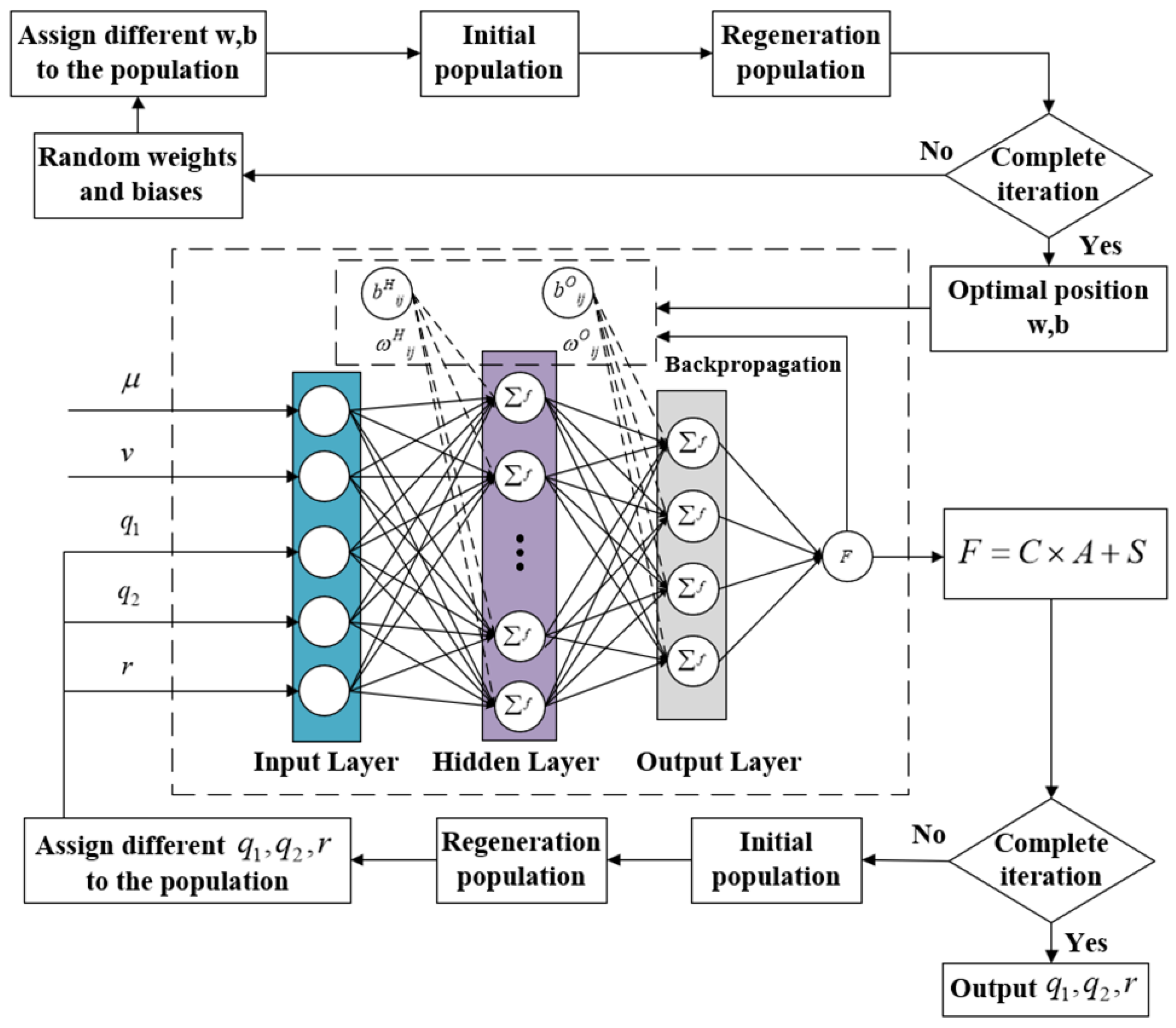
Under varying driving conditions, such as changing road adhesion coefficients and vehicle speeds, there exists a complex nonlinear relationship between the parameters of the MPC controller and the accuracy and stability of path tracking. Specifically, the weight coefficients for lateral tracking error and heading error are denoted as $q_1$ and $q_2$, respectively; the weight coefficient for control increment is denoted as $r$. When vehicle stability is low, increasing the weight on lateral tracking error to improve accuracy may cause instability, which results in larger lateral errors. Therefore, adaptive adjustment of controller parameters under varying driving conditions is essential to maintain both tracking accuracy and stability. Leveraging the universal approximation capability of three-layer neural networks, this paper employs such a network to model the nonlinear mapping between MPC weight parameters and path tracking accuracy and stability under varying driving conditions. A fitness function is designed, and the Snake Optimization Algorithm is utilized to iteratively optimize the MPC weight parameters.

To avoid local optima in gradient descent-based error back-propagation, the Snake Optimization Algorithm is utilized for global search. This helps improve prediction accuracy and generalization by optimizing the neural network’s weights and biases. Vehicle speed, road adhesion coefficient, and MPC weight coefficients serve as the neural network’s inputs, while the maximum lateral error, average lateral error, maximum centroid sideslip angle, and maximum yaw rate are defined as the outputs, as shown in Figure 3.

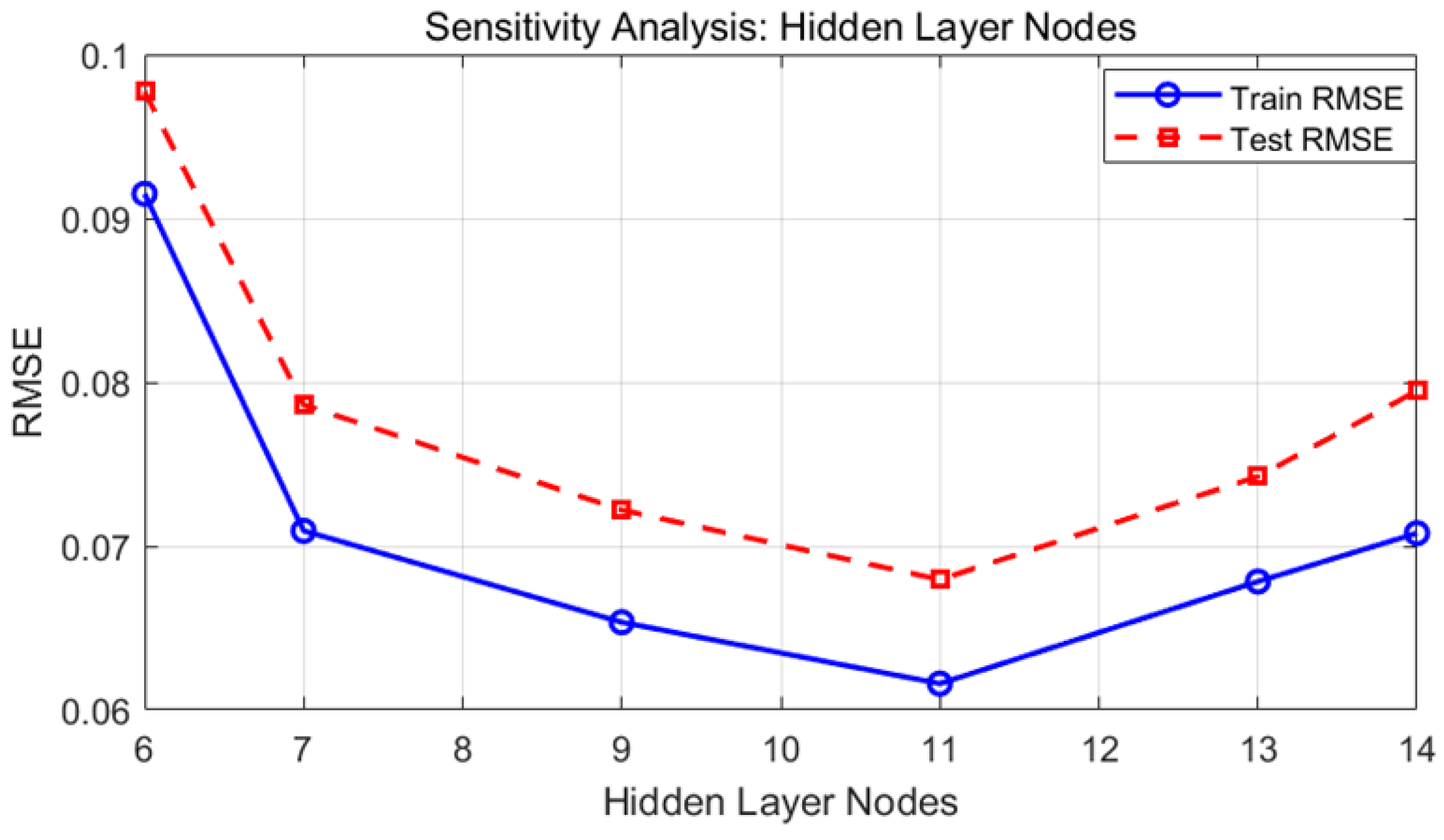
To determine the number of hidden layer nodes in the neural network, an empirical formula $N_h=\sqrt{N_i\times N_o}+\alpha$ was used to narrow down the search range, where $N_h$ denotes the number of hidden nodes, $N_i$ the number of input nodes, $N_o$ the number of output nodes, $\alpha$ is a tuning parameter. A sensitivity analysis was conducted with the number of hidden nodes varying from 6 to 14. As shown in Figure 4, the RMSE values on both the training and testing datasets initially decrease and then increase as the number of hidden nodes increases. When the number of hidden nodes is 11, the test RMSE reaches its minimum. Consequently, 11 hidden nodes are adopted in this study as the final network structure to achieve a trade-off between prediction accuracy and computational efficiency. This configuration not only ensures prediction accuracy but also effectively prevents overfitting. The iteration limit is set to 1000, with a target error of $1\times {10}^{-6}$ and a learning rate of 0.001.

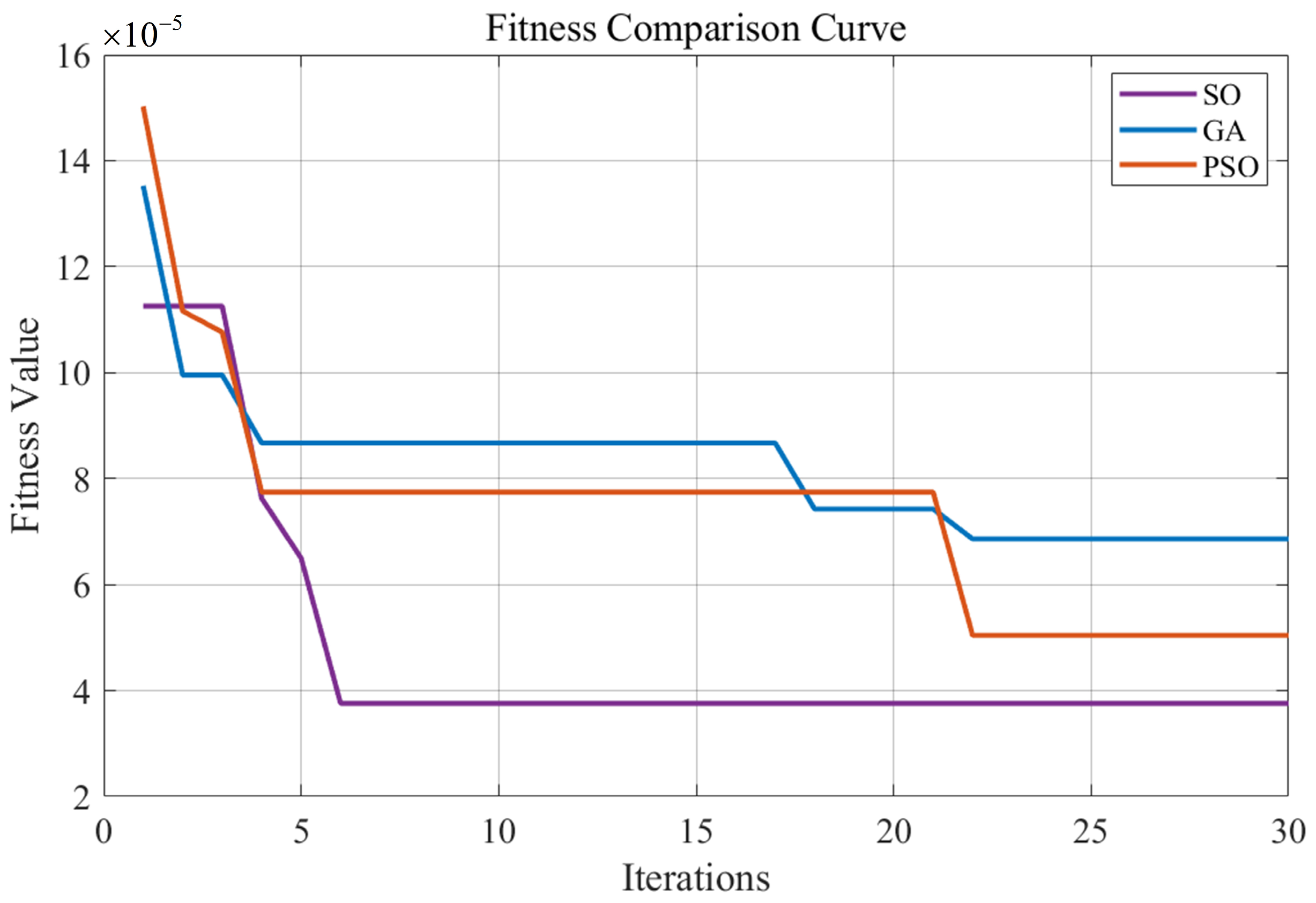
To evaluate the effectiveness of the proposed Snake Optimization (SO) algorithm for optimizing neural network weights and biases, a comparative study was conducted with two well-established methods: Genetic Algorithm (GA) and Particle Swarm Optimization (PSO). To ensure a fair comparison, all three algorithms were implemented under identical experimental settings. Specifically, the number of hidden layer neurons was fixed at 11, the learning rate was set to 0.001, the maximum number of training iterations was limited to 1000, and the target error threshold was defined as $1\times {10}^{-6}$. The convergence behavior of each algorithm during training is illustrated in Figure 5. The results indicate that the SO algorithm surpasses both GA and PSO in convergence efficiency and final prediction accuracy. In particular, when the convergence criteria were met, GA required 22 iterations to reach a final fitness value of $6.86\times {10}^{-5}$, while PSO also converged in 22 iterations with a final fitness of $5.04\times {10}^{-5}$. In contrast, SO achieved convergence in just 6 iterations, reaching a lower final fitness value of $3.75\times {10}^{-5}$. These outcomes demonstrate that SO not only converges more rapidly but also yields a more accurate solution, indicating superior parameter optimization capability and higher overall efficiency.

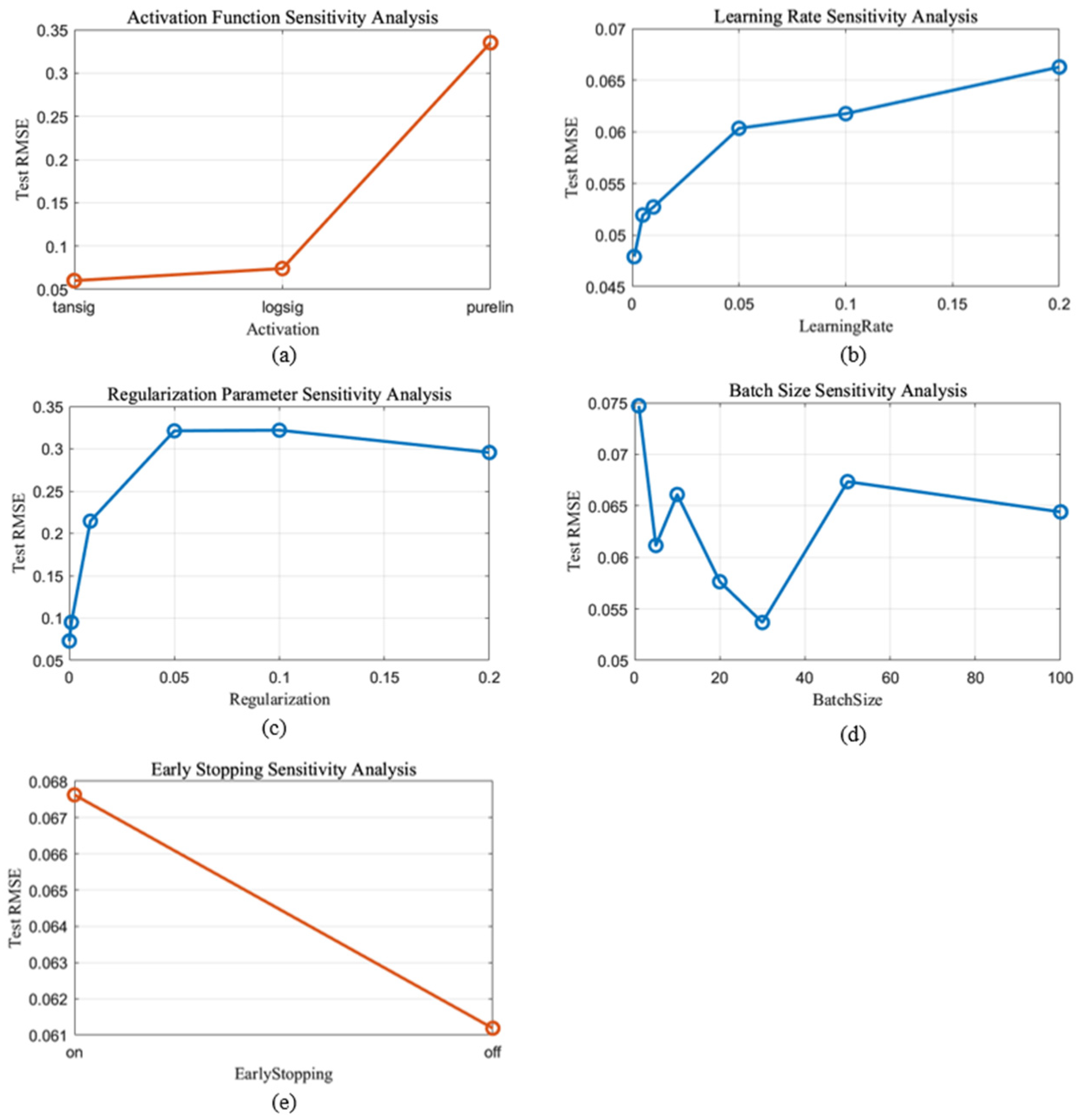
To enhance the overall performance and training stability of the neural network model, a systematic sensitivity analysis was conducted on several critical hyperparameters. These included the activation function, learning rate, regularization coefficient, batch size, and early stopping. The detailed results of this analysis are illustrated in Figure 6. The test root mean square error (Test RMSE) was used as the evaluation metric, with lower values indicating better generalization. Regarding the selection of activation functions, three commonly employed types were evaluated: hyperbolic tangent sigmoid (tansig), logarithmic sigmoid (logsig), and linear (purelin). The results demonstrated that the tansig function achieved the lowest Test RMSE of 0.06, suggesting its superior ability to capture non-linear relationships in the data for this regression task. The learning rate was explored over a range of values: 0.001, 0.01, 0.05, 0.1, 0.15, and 0.2. Among these, the network achieved optimal performance when the learning rate was set to 0.001, with a corresponding Test RMSE of 0.048. To mitigate overfitting and regulate model complexity, the regularization parameter was examined at values of 0.001, 0.05, 0.1, and 0.2. The best result was observed when the parameter was set to 0.001, yielding a Test RMSE of 0.075. The impact of batch size on training dynamics was also analyzed by testing values of 1, 5, 10, 20, 30, 50, and 100. A batch size of 30 resulted in the lowest Test RMSE of 0.054, indicating a favorable balance between convergence speed and stability. Furthermore, the early stopping strategy was evaluated by comparing training outcomes under enabled and disabled settings. Interestingly, disabling early stopping led to improved generalization, achieving a Test RMSE of 0.061. Based on these experimental findings, the final hyperparameter configuration adopted in this study included: the tansig activation function, a learning rate of 0.001, regularization parameter of 0.001, batch size of 30, and training without early stopping. This configuration provides an effective trade-off between generalization and training stability.

3.1. BP Neural Network Training

To enable the MPC controller to adapt to different driving conditions, the road surface is categorized into three types: dry, wet, and icy, with friction coefficients of 0.8, 0.5, and 0.3, respectively. The weight ranges for lateral, yaw angle, and control error are set from 1 to 100. The minimum and maximum speeds are set at 54 km/h and 120 km/h, respectively. A simulation platform is established to conduct MPC integrated control system simulations under various driving conditions, ultimately generating 2376 sample data points.

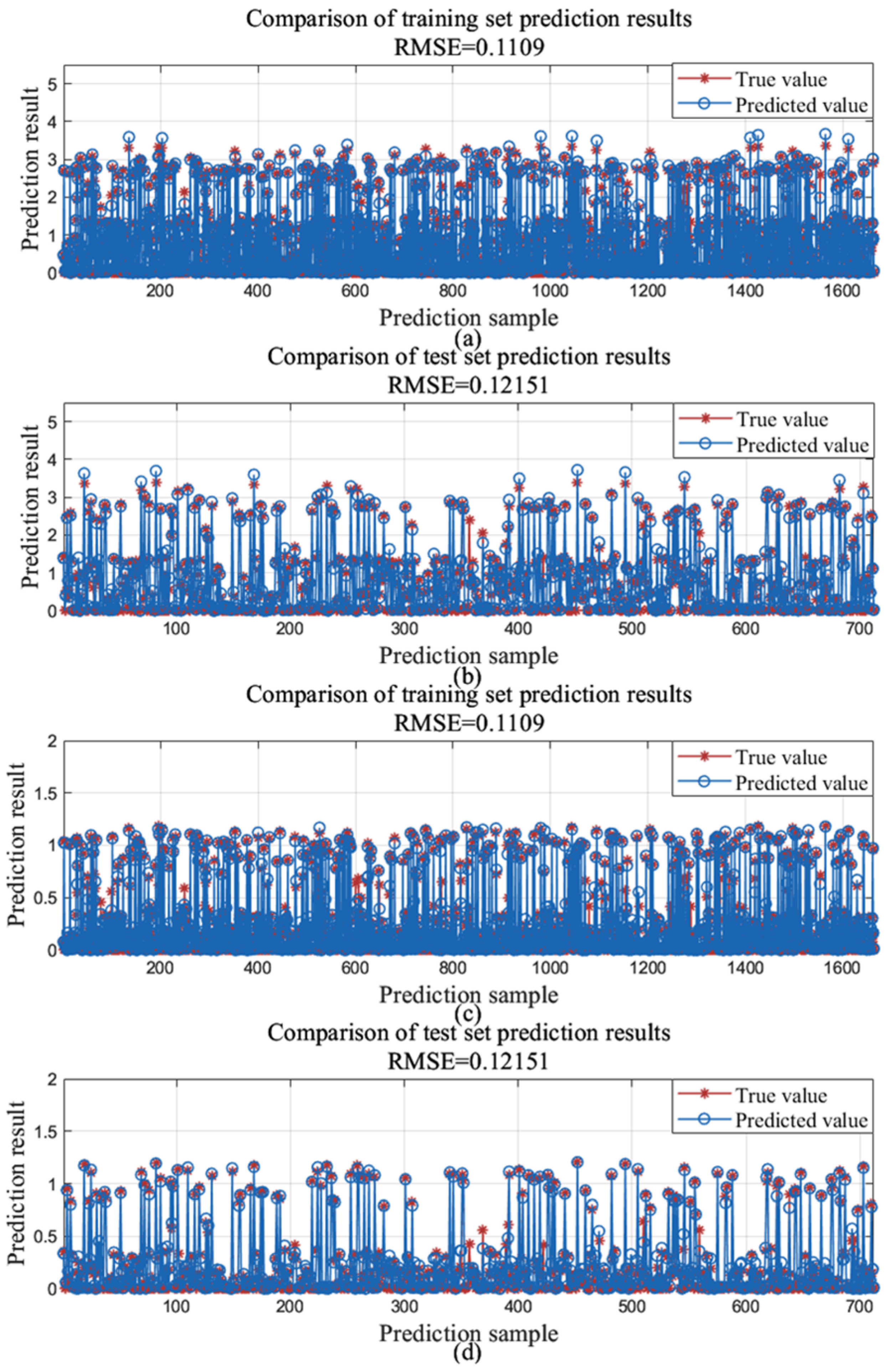
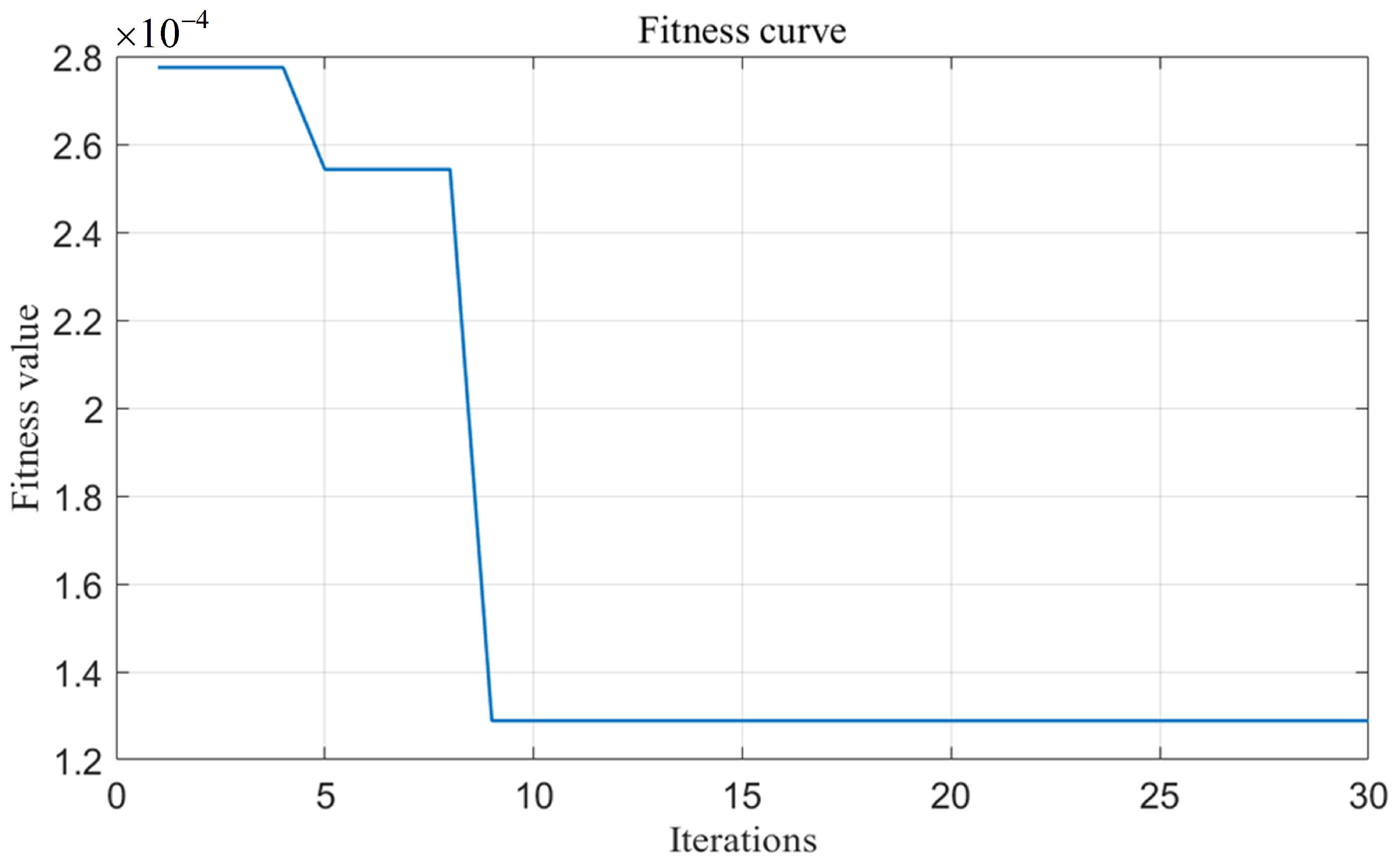
The forecasted outcomes for the training dataset input and output are presented in Figure 7a,c, while the predicted results for the test set input and output are shown in Figure 7b,d. In the figure, RMSE denotes the Root Mean Squared Error. The Snake algorithm optimized neural network parameters converged after the ninth iteration, with a fitness of 0.000128, as shown in Figure 8. The dataset was divided such that 70% was used for training and the remaining 30% was kept aside for testing. During model training, a subset of the training data was automatically selected for validation to assess learning performance and reduce the risk of overfitting. The test set was solely employed in the final evaluation stage to ensure unbiased performance assessment. The regression functions and correlation are presented in

Table 2. Results of Regression Models and Correlation Analysis.

	Regression Models	Correlation
Training Set	Prediction = target + 0.0045	0.98703
Validation Set	Prediction = target + 0.0015	0.99076
Test Set	Prediction = target + 0.0036	0.98797
All	Prediction = target + 0.0039	0.98775

. Regarding the training, validation, and testing datasets, the regression slopes remain at 1, with correlation coefficients exceeding 0.98, validating the reliability of the predictive model. Thus, the neural network effectively captures the relationship between MPC weight parameters and vehicle state.

To address the potential risk of overfitting and more thoroughly evaluate the generalization capability of the proposed neural network model, this study employed the K-fold cross-validation technique. Specifically, the entire dataset was randomly divided into five equal subsets (K = 5). In each iteration, one subset was used as the validation set, while the remaining four were used for training. This procedure was repeated five times, ensuring that each subset served as the validation set exactly once. The final performance metrics were obtained by averaging the results across all folds, thereby improving the robustness of the evaluation and reducing dependence on any single data split.

Model performance was assessed using the coefficient of determination (R²), which quantifies the proportion of variance in the observed data that is explained by the model’s predictions. The coefficient of determination is calculated as $R^2=1-{\displaystyle \frac{{\displaystyle {\sum }_{i=1}^n{(y_i-{\widehat{y}}_i)}^2}}{{\displaystyle {\sum }_{i=1}^n{(y_i-\overline{y})}^2}}}$, where $y_i$ is the observed value, ${\widehat{y}}_i$ is the predicted value, and $\overline{y}$ is the mean of the observed values. The results demonstrate that the model achieved an average coefficient of determination of 0.9879 on the training folds and 0.9863 on the validation folds, reflecting strong training stability and robust convergence without evident signs of overfitting.

3.2. Snake Optimization Algorithm

The Snake Optimization (SO) method is an optimization technique based on the foraging and reproductive behaviors of snakes. The reason for choosing SO in this study lies in its unique ability to dynamically balance global exploration and local exploitation, which is particularly advantageous for handling high-dimensional and complex problems. Through its two-phase design, SO avoids the premature convergence commonly seen in Genetic Algorithms (GA) and the tendency of Particle Swarm Optimization (PSO) to become trapped in local optima in multimodal problems. In the phase of food scarcity, SO performs extensive global exploration, increasing the likelihood of escaping local optima; when food is sufficient and the temperature is high, the algorithm shifts to local search around the target region, accelerating convergence and improving solution accuracy. Therefore, SO is well suited for solving optimization problems characterized by large search spaces and multiple local extrema, as in this study. The population size for the neural network parameter optimization using the SO algorithm is set to $n=30$, and the iteration count is set to $T=30$. In the first phase, when food is insufficient (i.e., food quality $Q(t)=0.5e^{{\displaystyle \frac{t-T}{T}}}<0.25$), the snake swarm explores and searches for food at random positions, updating their positions as described in Equation (17).

$$\left\{\begin{array}{l}{x}_{i,g}(t+1)=x_{i,g}(t)\pm c_1\times A_g(x_{\min }+(x_{\max }-x_{\min })\times rand)\\ A_g=\exp (-{\displaystyle \frac{f_{rand,g}}{f_{i,g}}})\end{array}\right.$$

(17)

where $x_{i,g}(t)$ represents the $i-th$ element of the position vector of an individual in the $t-th$ generation, where $g=f,m$ denotes either a female or male individual, and $rand$ represents a randomly generated number within the closed interval [0, 1]. $x_{\min }$, $x_{\max }$ define the lower and upper limits of the boundary values. $A_g$ represents the food-seeking ability of individuals in the population, while $f_{rand,g}$, $f_{i,g}$ represent the fitness of a randomly chosen individual and the $i-th$ individual, respectively.

In the second phase, when food is abundant but the temperature is too high (i.e., $Q>0.25$ and $T(t)=e^{-{\displaystyle \frac{t}{T}}}>0.6$), the snake swarm explores around the food and enters a local search phase, as illustrated in Equation (18).

$$\left\{\begin{array}{l}{x}_{i,g}(t+1)=x_{best}\pm x_Q\\ x_Q=c_2\times Temp\times rand(x_{best}-x_{i,j}(t))\end{array}\right.$$

(18)

In the equation, $x_{best}$ indicates the best individual’s position in the $t-th$ generation. If $Rand<0.6$, the population engage in battle mode, and individuals fight to obtain the best mate of the opposite sex, as described in Equation (19).

$$\left\{\begin{array}{l}{x}_{i,m}(t+1)=x_{i,m}(t+1)\pm x_{Fm}\\ x_{i,f}(t+1)=x_{i,f}(t+1)\pm x_{Ff}\\ x_{Fm}=c_2\times F_m\times rand\times (x_{best,f}-x_{i,m}(t))\\ x_{Ff}=c_2\times F_f\times rand\times (x_{best,m}-x_{i,f}(t))\end{array}\right.$$

(19)

When $Rand>0.6$, the population enter the mating mode, and their movement equation is given as follows:

$$\left\{\begin{array}{l}{x}_{i,m}(t+1)=x_{i,m}(t)\pm x_{Mm}\\ x_{i,f}(t+1)=x_{i,f}(t)\pm x_{Mf}\\ x_{Mm}=c_2\times M_m\times rand\times (Q\times x_{i,f}-x_{i,m}(t))\\ x_{Mf}=c_2\times M_f\times rand\times (Q\times x_{i,m}-x_{i,f}(t))\end{array}\right.$$

(20)

In the equation:

$$\left\{\begin{array}{l}{F}_m=\exp (-{\displaystyle \frac{f_{best,f}}{f_{i,m}}})\\ F_f=\exp (-{\displaystyle \frac{f_{best,m}}{f_{i,f}}})\end{array}\right.; \left\{\begin{array}{l}{M}_m=\exp (-{\displaystyle \frac{f_{i,f}}{f_{i,m}}})\\ M_f=\exp (-{\displaystyle \frac{f_{i,m}}{f_{i,f}}})\end{array}\right.$$

where $f_{best,m}$, $f_{best,f}$ signify the optimal fitness levels in the male and female groups, while $f_{i,m}$ and $f_{i,f}$ represent the fitness scores of the $i-th$ individual within the male and female populations. In mating mode, there is a 50% probability of generating a new individual, which will replace the least fit individual in the population.

$$x_{worst,g}(t+1)=x_{\min }+rand\times (x_{\max }-x_{\min })$$

(21)

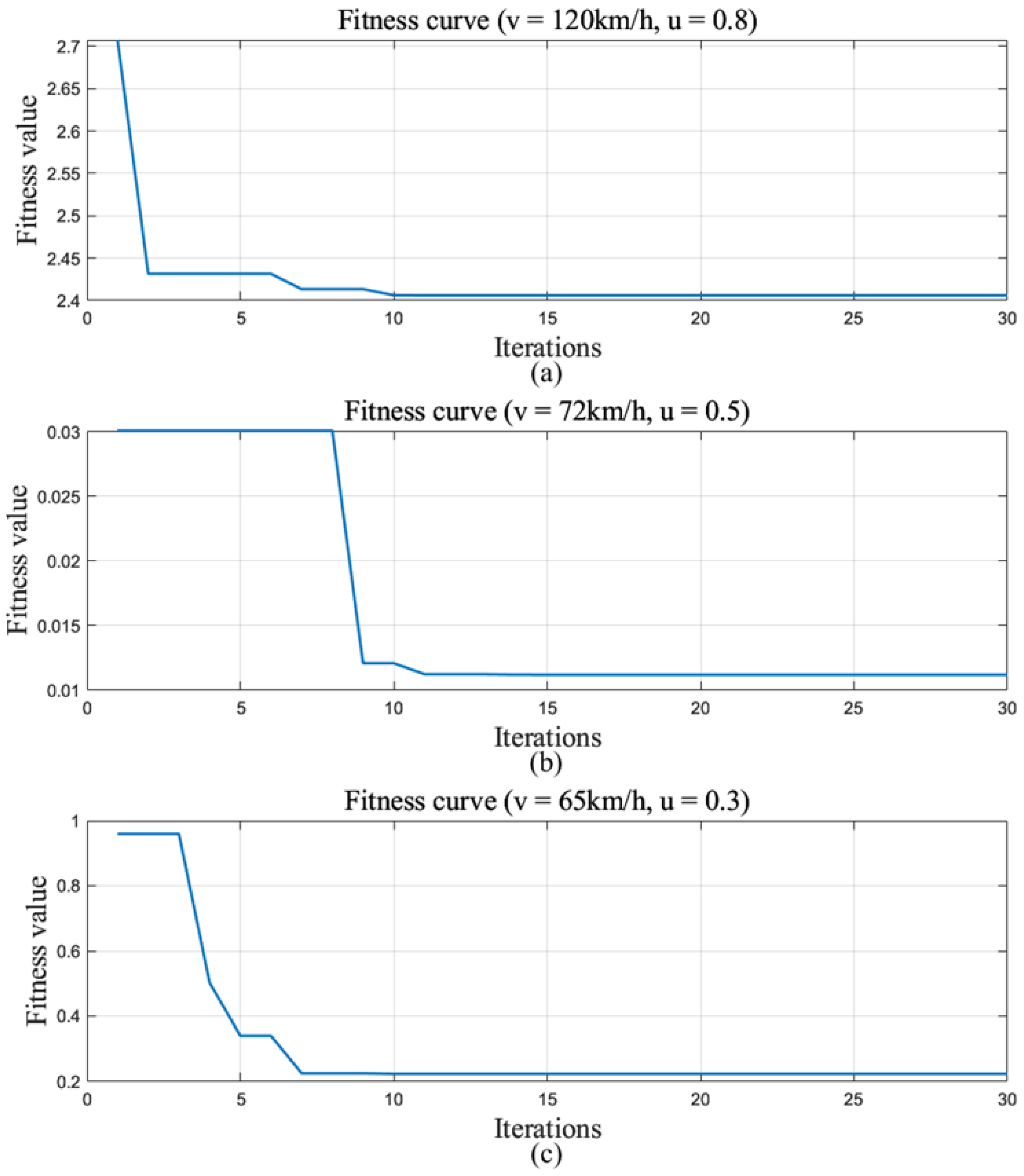
Based on the results generated by the neural network model, the maximum and average lateral errors are normalized and represented as $A$, while the maximum centroid slip angle and maximum yaw rate are normalized and represented as $S$. The fitness function $F=C\times A+S$ is designed, where $C$ is a constant. The Snake Algorithm is applied to iteratively optimize the controller parameters to ensure tracking accuracy and stability. The population size for controller parameter optimization is set to 30, with a maximum iteration count of 30, and position limits are set between −1 and 1. The constants $c_1$, $c_2$ are set to 0.5 and 2, respectively.

4. Stability Control Strategy

4.1. Phase Plane Control Domain Division

Based on Equation (4), using the centroid side slip angle and yaw rate as stability control objectives, the nonlinear vehicle model with direct yaw moment incorporated is derived as follows:

$$\left\{\begin{array}{l}\dot{\beta }={\displaystyle \frac{k_1+k_2}{m{v}_x}}\beta +({\displaystyle \frac{l_f{k}_1-l_r{k}_2}{m{v_x}^2}}-1)\gamma -{\displaystyle \frac{k_1}{m{v}_x}}{\delta }_f-{\displaystyle \frac{k_2}{m{v}_x}}{\delta }_r\\ \dot{\gamma }={\displaystyle \frac{l_f{k}_1-l_r{k}_2}{I_z}}\beta +{\displaystyle \frac{{l_f}^2{k}_1+{l_r}^2{k}_2}{I_z{v}_x}}\gamma -{\displaystyle \frac{l_f{k}_1}{I_z}}{\delta }_f+{\displaystyle \frac{l_r{k}_2}{I_z}}{\delta }_r+{\displaystyle \frac{1}{I_z}}{M}_1\end{array}\right.$$

(22)

At elevated speeds, the vehicle experiences increased lateral acceleration, and the tires primarily function under non-linear conditions. In this research, the Magic Tire Model combined with the phase plane method is utilized to investigate the vehicle’s nonlinearity under extreme conditions. The model is expressed as shown in Equation (23).

$$F_{yi}=F_{zi}{D}_y\sin (C_{y}a\tan (B_y{\alpha }_i+E_y(B_y{\alpha }_i-a\tan (B_y{\alpha }_i))))$$

(23)

The side force of the wheel is denoted as $F_{yi}$, while the vertical load is denoted by $F_{zi}$. ${\alpha }_i$ is the tire’s sideslip angle, $i=f,r$. $D_y$, $C_y$, $B_y$ and $E_y$ are the fitting coefficients.

When the vehicle is in motion, the normal forces exerted on the front and rear tires are formulated in Equation (24).

$$\left\{\begin{array}{l}{F}_{zf}=mg{l}_r/(l_f+l_r)\\ F_{zr}=mg{l}_f/(l_f+l_r)\end{array}\right.$$

(24)

The phase plane method does not require solving nonlinear equations. Instead, it visually describes the system’s stability through phase trajectories. The state points within the stable region, determined by the double-line approach, converge to the origin, while the points in the unstable region diverge. 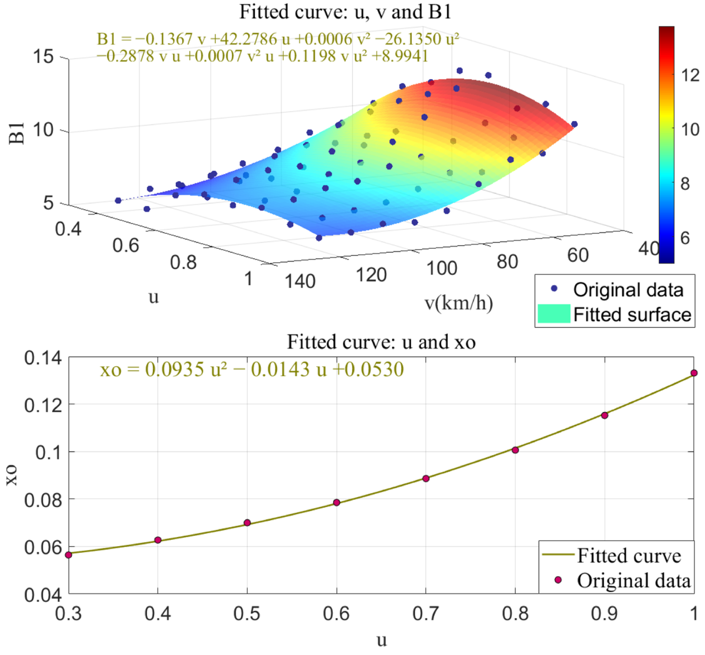When the steering angle is minor, the intercept of the stability threshold is significantly influenced by the road friction coefficient, while the slope is affected by both the travelling speed and the road friction coefficient [33]. Therefore, in this study, the vehicle speed is incremented by 9 km/h, spanning from 54 km/h to 126 km/h, and the road adhesion value is assigned to fixed intervals of 0.1, ranging from 0.3 to 1, resulting in 72 sample sets. The boundary parameters, including the slope $B_1$ and the intercept $x_0$, are fitted using the least squares method, as shown in Figure 9. The parameters $B_1$ and $B_2$, obtained through least squares fitting, yielded coefficients of determination $R^2$ of 0.9575 and 0.9542, respectively. The RMSE of the fitting results for $B_1$ and $B_2$ are 0.6056 and 0.000802, respectively. The results indicate that the constructed model effectively captures the data characteristics and fits the observed data with high fidelity. The relative errors, calculated based on the magnitudes of the two datasets, are 4.04% and 1.04%, respectively. Some data is shown in

Table 3. Fitting parameters for a road surface friction coefficient of 0.8 at different speeds.

Vehicle Speed (m/s)	${\mathit{B}}_1$	${\mathit{B}}_2$
15.0	12.54	1.26
17.5	11.75	1.18
20.0	10.71	1.07
22.5	9.84	0.98
25.0	9.39	0.94
27.5	8.57	0.86
30.0	8.30	0.83
32.5	7.73	0.77
35	7.37	0.74

. The expressions for the boundary parameters $B_1$ and $B_2$ are given by Equation (25).

$$\left\{\begin{array}{l}\left|\dot{\beta }+B_1\beta \right|\le B_2\\ B_1=0.0006v^2-26.135{\mu }^2+0.0007v^2\mu +0.1198v{\mu }^2\\ -0.2878v\mu -0.1367v+42.2786\mu +8.9941\\ B_2=x_0{B}_1=(0.094{\mu }^2-0.014\mu +0.053)B_1\end{array}\right.$$

(25)

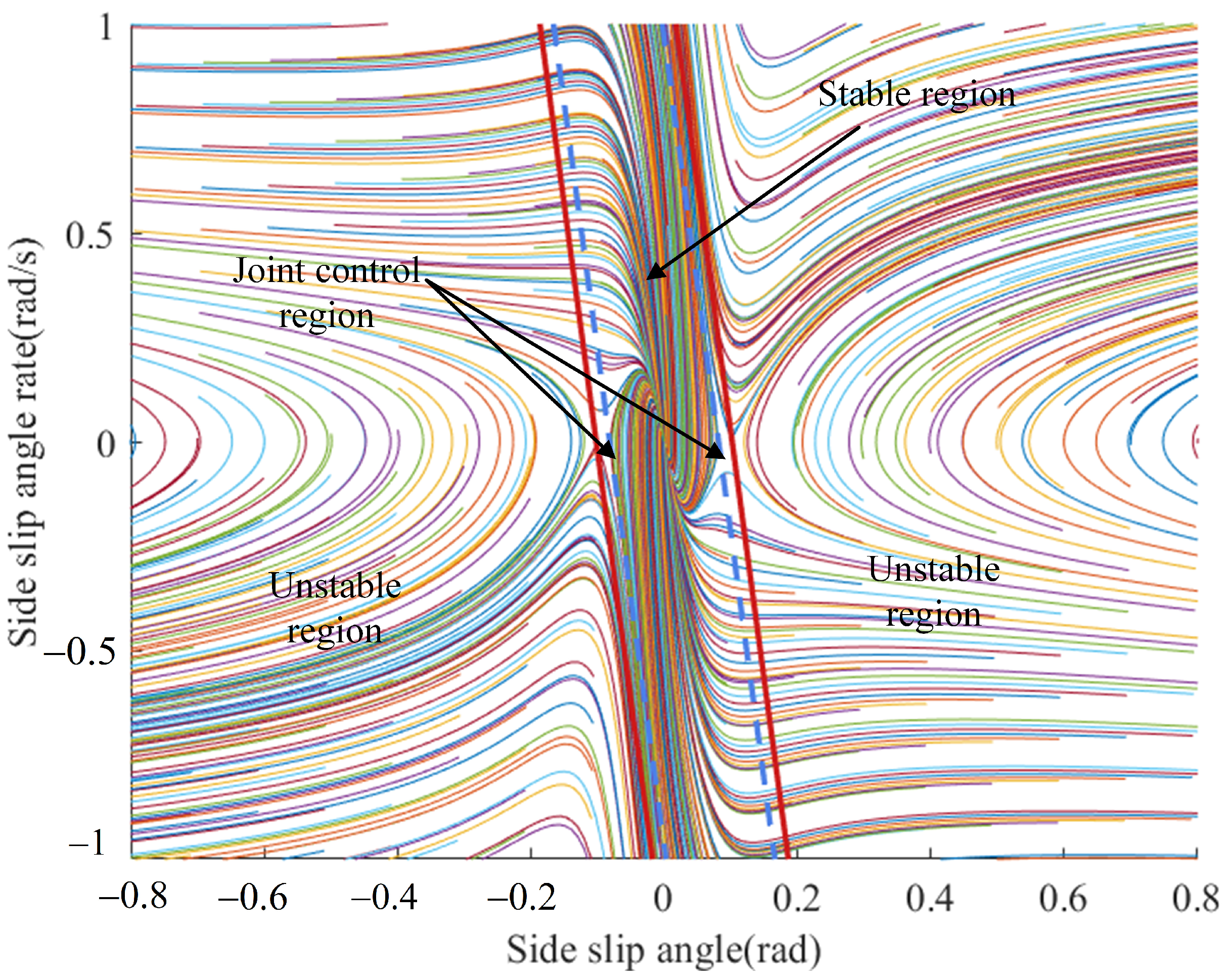
To accelerate the convergence process, the stable region is further divided into stable region and joint control domain. The region division formula is expressed by Equation (26).

$$\left\{\begin{array}{ll}\left|{\displaystyle \frac{B_1}{B_2}}\beta +{\displaystyle \frac{1}{B_2}}\dot{\beta }\right|\le \mu & (stable region control domain)\\ \mu \le \left|{\displaystyle \frac{B_1}{B_2}}\beta +{\displaystyle \frac{1}{B_2}}\dot{\beta }\right|\le 1& (joint control domain)\\ \left|{\displaystyle \frac{B_1}{B_2}}\beta +{\displaystyle \frac{1}{B_2}}\dot{\beta }\right|\ge 1& (unstable region control domain)\end{array}\right.$$

(26)

Given the vehicle’s state and using Equations (21)–(25), the system’s phase trajectory is plotted to obtain the $\beta -\dot{\beta }$ phase plane diagram. Figure 10 displays the phase trajectory when the steering angle is 0 degrees, with a speed of 72 km/h and a road friction value of 0.8.

In the $\beta -\dot{\beta }$ phase plane diagram, the separation from the state point to the stability boundary indicates the vehicle’s instability level. Inside the stable region, the instability degree is zero, as shown in Equation (27).

$$e(d)=\left\{\begin{array}{l}{\displaystyle \frac{\left|B_1\beta +\dot{\beta }-B_2\right|}{\sqrt{1+{B_1}^2}}},(B_1\beta +\dot{\beta }>B_2)\\ 0,(\left|B_1\beta +\dot{\beta }\right|\le B_2)\\ {\displaystyle \frac{\left|B_1\beta +\dot{\beta }+B_2\right|}{\sqrt{1+{B_1}^2}}},(B_1\beta +\dot{\beta }<-B_2)\end{array}\right.$$

(27)

4.2. Sliding Mode Controller Design

The primary strength of the Sliding Mode Controller (SMC) lies in its robustness to vehicle nonlinearities and external disturbances [34]. The control variable is defined as the weighted sum of the deviations of the actual side slip angle and yaw rate from their respective reference values, as shown in Equation (28).

$$e=P{e}_{\beta }+(1-P)e_{\gamma }$$

(28)

To enhance the precision of the approximation process, an integral element is added to the sliding surface.

$$S=e+c{\displaystyle {\int }_0^{t}edt}=P{e}_{\beta }+(1-P)e_{\gamma }+c{\displaystyle {\int }_0^{t}P{e}_{\beta }+(1-P)e_{\gamma }}dt$$

(29)

The sliding mode approximation adopts an exponential convergence rate.

$$\dot{S}=-\epsilon \mathrm{sgn}(S)-KS=P{\dot{e}}_{\beta }+(1-P){\dot{e}}_{\gamma }+cP{e}_{\beta }+c(1-P)e_{\gamma }$$

(30)

In the sliding mode controller, the parameter $c$ is a key factor in regulating the system’s response characteristics, primarily influencing both the convergence rate and the amplitude of chattering. While a larger value of $c$ can accelerate convergence to the steady state, it may also induce high-frequency oscillations, which can degrade control accuracy and potentially affect the robustness of the controller. To balance dynamic performance and system stability, the parameter $c$ was gradually increased while comprehensively considering the impact of system oscillations. After multiple rounds of simulation and experimental comparisons, the parameter $c$ was ultimately determined to be set at 0.5. By combining Equation (22) with Equations (28)–(30), the yaw moment $M_1$ is formulated as follows:

$$M_1=-I_z\left[{\displaystyle \frac{l_f{k}_1-l_r{k}_2}{I_z}}\beta +{\displaystyle \frac{{l_f}^2{k}_1+{l_r}^2{k}_2}{I_z{v}_x}}\gamma -{\displaystyle \frac{l_f{k}_1}{I_z}}{\delta }_f+{\displaystyle \frac{l_r{k}_2}{I_z}}{\delta }_r-{\dot{\gamma }}_d+{\displaystyle \frac{P}{1-P}}(\dot{\beta }-{\dot{\beta }}_d)+c(\gamma -{\gamma }_d)+{\displaystyle \frac{cP}{1-P}}(\beta -{\beta }_d)+{\displaystyle \frac{\epsilon sign(S)+kS}{1-P}}\right]$$

(31)

In the above equation, $\epsilon$ represents the thickness of the sliding mode controller boundary layer, while $K$ denotes the convergence rate exponent. Both $\epsilon$ and $K$ are positive numbers. $P$ is defined as:

$$P=\left\{\begin{array}{l}1-{\displaystyle \frac{2h}{H}} 0<\mathrm{h}<0.4\mathrm{H}\\ 0.2 0.4<\mathrm{h}<0.5\mathrm{H} \end{array}\right.$$

(32)

where $h$ denotes the separation between the phase plane state point and the nearest stability limit, and $H$ represents the spacing between stable boundaries. The continuous function is employed to replace the sign function in order to suppress system chattering, as shown in Equation (33).

$$sat(S)=\left\{\begin{array}{ll}1& S>\Delta \\ \lambda S& |S|\le \Delta , \Delta ={\displaystyle \frac{1}{\lambda }}\\ -1& S<-\Delta \end{array}\right.$$

(33)

Based on Lyapunov stability theory, the system is asymptotically stable if the positive-definite scalar function $V(x)=S^2/2$ has a negative-definite time derivative. The Lyapunov function is defined as:

$$\dot{V}=\dot{S}\times S=-\epsilon \mathrm{sgn}(S)\times S-K{S}^2=-\epsilon \left|S\right|-K{S}^2$$

(34)

When $S>0$ or $S<0$, $\dot{V}=-\epsilon S-K{S}^2<0$; When $S=0$, $\dot{V}=0$. Therefore, $\dot{V}\le 0$ always holds, which proves that the system is asymptotically stable.

Once the vehicle enters the instability region, the control objective at this point is to minimize the instability degree $e(d)$. Using $e(d)$ as the input to the controller, the PID controller is utilized to calculate the needed yaw moment within the instability region, with the output being the yaw moment $M_2$.

$$M_2=k_{p}e(d)+k_i{\displaystyle \int e(d)dt+}{k}_d{\displaystyle \frac{de(d)}{dt}}$$

(35)

PID parameter tuning was conducted under high-instability and low-adhesion driving conditions. Specifically, a road friction coefficient of $\mu$ = 0.3 and a vehicle speed of 60 km/h were selected as the test conditions. The proportional gain was gradually increased to achieve a rapid response to the onset of instability, until the system approached the instability boundary. This ensured quick system response while maintaining an adequate gain margin. The integral term was introduced to eliminate residual yaw rate errors, and the derivative term was tuned to suppress oscillations near the stability boundary. Based on multiple simulation iterations, the final controller parameters were set to $k_p$ = 8000, $k_i$ = 90, and $k_d$ = 50. Finally, with the set values fluctuating by $\pm 25\%$, the controller maintained stable performance., indicating robustness to parameter variations. Incorporating the phase plane region division, a weighting coefficient $\lambda ={\displaystyle \frac{x-1}{\mu -1}}$ is introduced in the joint control domain, where $\mu$ represents the road adhesion coefficient and $x=\left|{\displaystyle \frac{1}{c}}\dot{\beta }+{\displaystyle \frac{k}{c}}\beta \right|$. The total additional yaw moment is calculated as follows:

$$M_z=\lambda M_1+(1-\lambda )M_2$$

(36)

According to vehicle stability theory, when the centroid slip angle is small, the vehicle’s stability is primarily affected by the yaw rate. In contrast, when the slip angle becomes large, stability mainly depends on the slip angle itself. Therefore, the integrated error-weighted distribution method, combined with coordinated control regions and designed using the phase-plane approach, can adapt the torque distribution under various driving conditions.

4.3. Optimal Distribution of Longitudinal Driving Torque and Additional Yaw Moment

The optimal distribution is a torque allocation strategy that considers three key factors: tire utilization, motor drive torque, and road friction [35]. This strategy aims to meet the required total longitudinal driving force $F_x$. Simultaneously, the additional yaw moment $M_z$, assigned by the upper-level controller, is allocated to each wheel. Through this allocation, direct yaw moment control is achieved. The method can be expressed as shown in Equation (37).

$$\left\{\begin{array}{l}{F}_{xq1}=F_x={\displaystyle \frac{T}{R_w}}\\ F_{xm1}={\displaystyle \frac{2M_z}{B}}\end{array}\right.$$

(37)

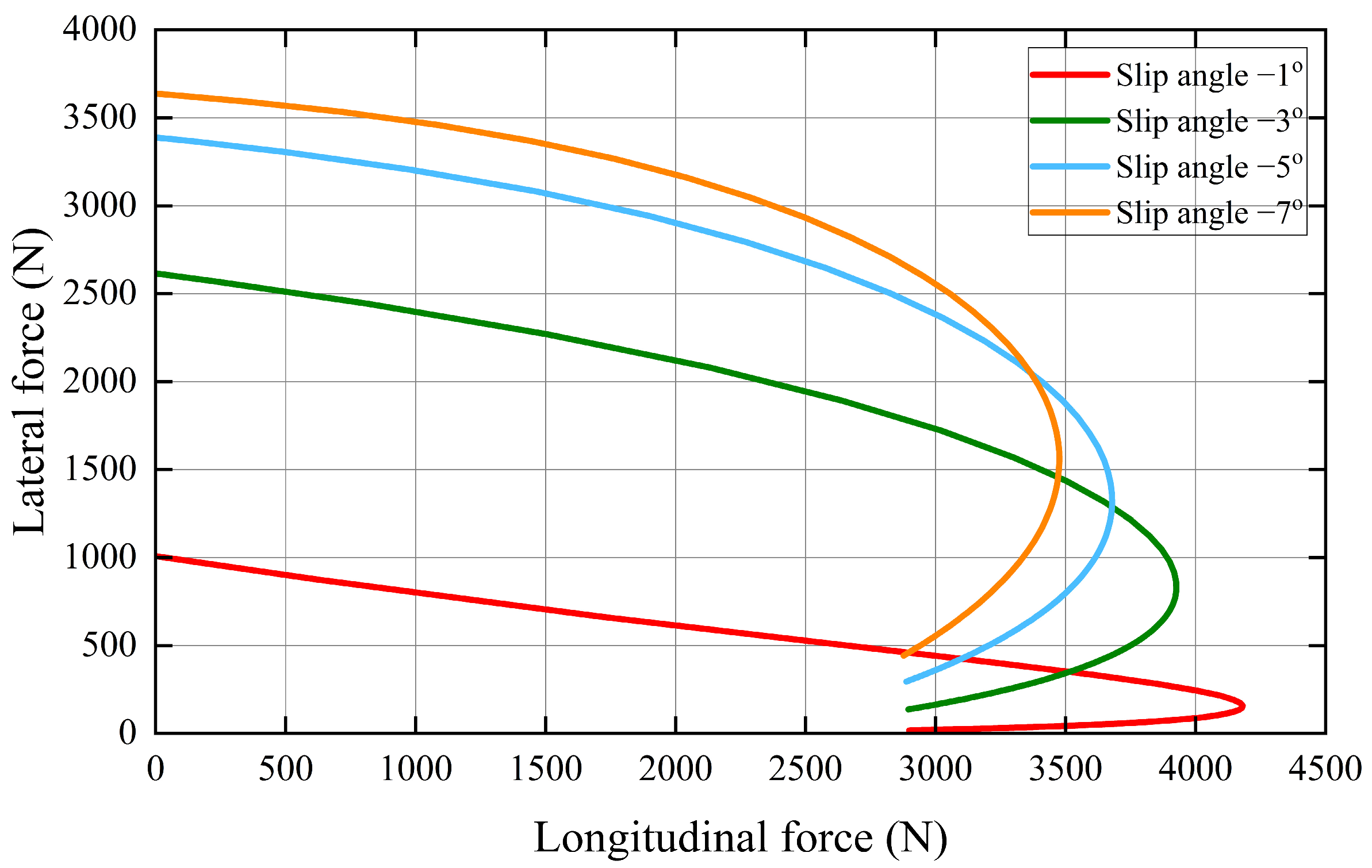
where $F_{xq1}$ denotes the control effect of the longitudinal driving force, and $F_{xm1}$ represents the control effect of the stability controller. $B$ denotes track width. The coupling between the longitudinal and lateral forces can be further illustrated by the friction ellipse model, as shown in Figure 11. According to the friction ellipse theory, the lateral force of a tire decreases as the longitudinal force increases. The upper limit of the lateral force is inversely proportional to the limit of the longitudinal force, thus indicating that there is a coupling between the longitudinal and lateral forces of the tire. To coordinate the longitudinal control with the stability control, $w_1$ and $w_2$ are introduced. The adjusted $F_{xq1}$ and $F_{xm1}$ are expressed as:

$$\left\{\begin{array}{l}{F}_{xq2}=w_1{F}_{xq1}\\ F_{xm2}=w_2{F}_{xm1}\end{array}\right.$$

(38)

Introducing the weighting coefficient $\eta$ transforms the optimization problem for solving $w_1$ and $w_2$ into a single-objective optimization problem, as shown in Equation (39).

$$\begin{array}{l}\max f(w_1,w_2)=\eta w_1+(1-\eta )w_2\\ st\left\{\begin{array}{l}0\le w_1,w_2\le 1\\ -2(A_{fl}+A_{rl})\le F_{xq2}+F_{xm2}\le 2(A_{fl}+A_{rl})\\ -2(A_{fr}+A_{rr})\le F_{xq2}-F_{xm2}\le -2(A_{fr}+A_{rr})\end{array}\right.\end{array}$$

(39)

where $A_i=\sqrt{{(\mu F_{zi})}^2+{F_{zi}}^2}$, $(i=fl,fr,rl,rr)$, and $F_{zi}$ signifies the vertical force on the tire. The larger the value of $\eta (0<\eta <1)$, the greater the contribution of the longitudinal controller, and conversely, the greater the contribution of the stability controller. Considering the vehicle’s instability and road adhesion coefficient, parameter $\eta$ is designed using the sigmoid function, as expressed by:

$$\eta ={\displaystyle \frac{1}{1+e^{10e(d)-2\mu }}}$$

(40)

The parameter $\eta$ is formulated as a sigmoid-type exponential function to represent the nonlinear and gradual variation in the coupling between the longitudinal and lateral forces of the tire. When the phase-plane instability metric $e(d)$ is low, indicating near-stable tire conditions, and the road friction coefficient $\mu$ is relatively high, $\eta$ approaches 1. This suggests that the longitudinal force has a limited influence on the lateral force, meaning the coupling between these forces is weak. Conversely, when $e(d)$ increases, indicating greater instability, or $\mu$ decreases, indicating smoother road surfaces, $\eta$ decreases. This shows that the longitudinal force has a stronger suppressive effect on the lateral force. This behavior reflects the dynamic coupling characteristics of tire forces under varying operating conditions.

Finally, considering the restrictions of peak motor torque and road adhesion, the driving torque delivered to each tire is determined. The cost function and constraints for optimal wheel torque allocation are formulated using a quadratic programming algorithm as follows:

$$\begin{array}{l}\min J={\displaystyle \sum _{i=fl,fr,rl,rr}\frac{{\zeta }_i{F_{xi}}^2}{{(\mu F_{zi})}^2}}\\ \left\{\begin{array}{l}{F}_{xi}<\mu F_{zi}\\ {\displaystyle \frac{T_{\min }}{r_w}}\le F_{xi}\le {\displaystyle \frac{T_{\max }}{r_w}}\\ F_{fl}+F_{fr}+F_{rl}+F_{rr}=F_{xq2}\\ F_{xfr}-F_{xfl}+F_{xrr}-F_{xrl}=F_{xm2}\end{array}\right.\end{array}$$

(41)

To further enhance vehicle stability and account for the vehicle’s understeer characteristics, the front wheel weight is set to 1, while the rear wheel weight is derived from phase-plane analysis, as shown in Equation (42).

$${\zeta }_{3,4}=\left\{\begin{array}{ll}1+\left|\beta \right|{\displaystyle \frac{B_1}{B_2}}& \left|\beta \right|\le {\displaystyle \frac{B_2}{B_1}}\\ 2& \left|\beta \right|>{\displaystyle \frac{B_2}{B_1}} \end{array}\right.$$

(42)

5. Results and Discussion

In this part, to assess the performance of the introduced control approach, a CarSim/Simulink joint simulation platform is established. Double line change path and slalom path are set as reference trajectories. Controller A denotes the proposed control system developed in this study. For comparison, three traditional controllers, Controller B (a traditional fixed-parameter model predictive controller), Controller C (a linear quadratic regulator, LQR), and Controller D (a sliding-mode rear-wheel active steering controller based on a single-point look-ahead driver model), are also implemented. The basic vehicle parameters employed in this study are presented in

Table 4. Basic vehicle parameters.

Parameters	Units	Value
Vehicle mass	$\mathrm{k}\mathrm{g}$	1412
Distance from the front axle to the mass center	$\mathrm{m}$	1.015
Distance from the rear axle to the mass center	$\mathrm{m}$	1.895
Track width	$\mathrm{m}$	1.675
Vehicle yaw moment of inertia	$\mathrm{k}\mathrm{g}\cdot {\mathrm{m}}^2$	1536.7
Effective rolling radius	$\mathrm{m}$	0.325
Front tire stiffness cornering	$\mathrm{N}/\mathrm{r}\mathrm{a}\mathrm{d}$	134,035
Rear tire stiffness cornering	$\mathrm{N}/\mathrm{r}\mathrm{a}\mathrm{d}$	77,802
Tire rotational inertia	$\mathrm{k}\mathrm{g}\cdot {\mathrm{m}}^2$	1.5

. The values of the control weight parameters under various driving conditions are summarized in

Table 5. Controller parameters.

Vehicle Speed (km/h)	Road Friction Coefficient	${\mathit{q}}_1$	${\mathit{q}}_2$	$\mathit{R}$
120	0.8	1	100	$diag(43,43,43)$
72	0.5	45	100	$diag(45,45,45)$
65	0.3	1	100	$diag(41,41,41)$

.

The lane-change maneuver at the high-speed dry road conditions and low-speed slippery road conditions, as well as the sharp turn maneuver under low-speed icy and snowy road conditions, were set up to validate the control strategy introduced in this paper. These three scenarios were used to verify that the introduced control strategy can ensure high precision and stability in tracking the target trajectory under different driving conditions. Figure 12a–c show the fitness curve variations during the iterative calculation process of the Snake algorithm after assigning values to the offline-trained model under the given driving conditions. The fitness curves in Figure 12a,b converge on the 10th and 11th iterations, with fitness values of 2.40628 and 0.01125, respectively. The fitness curve in Figure 12c converges on the 7th iteration, with a fitness value of 0.22572.

5.1. High-Speed Double Lane Change Maneuver

To evaluate the performance of the proposed path tracking controller under high-speed conditions, a lane-change and overtaking scenario on a dry road surface is simulated. The road friction coefficient is set to 0.8, and the vehicle maintains a constant speed of 120 km/h during the maneuver. The reference path is a typical double lane-change trajectory, with a total longitudinal length of 240 m and a lateral displacement of 3.6 m, forming a curve composed of two connected lateral shifts. The corresponding simulation results are shown in Figure 13, while the statistical results are presented in

Table 6. Statistical Results of High-Speed Double Lane Change Maneuver.

	Maximum Tracking Error (m)	Mean Tracking Error (m)	Maximum CG Sideslip Angle (rad)	Mean CG Sideslip Angle (rad)	Maximum Yaw Rate (rad/s)	Mean Yaw Rate (rad/s)
Control A	0.54	0.142	0.024	0.001	0.28	0.08
Control B	0.95	0.304	0.125	0.032	0.51	0.16
Control C	1.18	0.253	0.131	0.031	0.77	0.17
Control D	0.56	0.153	0.052	0.013	0.17	0.04

.

From Figure 13a, the lateral errors of Controller A and Controller D appear nearly identical, with a peak lateral deviation of approximately 0.54 m, which is significantly lower than those of Controller B and Controller C. The maximum lateral error of Controller C reaches 1.18 m, showing the worst tracking performance. Compared to the fixed-weight MPC controller, Controller A reduces the maximum lateral error by approximately 40%, demonstrating significant optimization. Figure 13b shows that although Controller A does not exhibit a significant advantage over Controller D in tracking performance, its maximum centroid side-slip angle, at around 0.024 rad, is the smallest among the four approaches. This demonstrates that the introduced method significantly enhances the vehicle’s lane-changing stability under high-speed conditions.

Figure 13c shows that the peak yaw rate of Controller A reaches 0.28 rad/s, with an average yaw rate of 0.08 rad/s, slightly higher than that of Controller D, but much lower than those of Controller B and Controller C. From the phase plane plot in Figure 13e, it is apparent that the phase trajectories of Controller A and Controller D are within the stable region and more concentrated compared to the other controllers. The stability of controller C is the worst, and certain state points exceed the stability boundary. The phase plane plot visually demonstrates that the introduced control method greatly enhances the vehicle stability of the MPC controller under high-speed maneuver. Figure 13d presents the drive torque outputs of each wheel, where the optimal distribution strategy is designed to coordinate the total driving force and extra yaw moment, achieving direct yaw moment control to sustain vehicle body stability. Figure 13f shows the path tracking performance of each controller, with Controllers A and D aligning more closely with the target trajectory, while the other controllers exhibit larger lateral deviations.

5.2. Slippery Road Double Lane Change Maneuver

The low-adhesion double-lane-change maneuver serves to simulate vehicle overtaking maneuvers on a wet, slippery road in rainy conditions. The road friction coefficient is assigned a value of 0.5, and the vehicle travels at 72 km/h. Simulation results are presented in Figure 14, while the statistical results are summarized in

Table 7. Statistical Results of Medium-Speed Double Lane Change Maneuver.

	Maximum Tracking Error (m)	Mean Tracking Error (m)	Maximum CG Sideslip Angle (rad)	Mean CG Sideslip Angle (rad)	Maximum Yaw Rate (rad/s)	Mean Yaw Rate (rad/s)
Control A	0.01	0.002	0.008	0.001	0.25	0.05
Control B	0.08	0.012	0.032	0.003	0.30	0.05
Control C	0.69	0.144	0.014	0.002	0.23	0.05
Control D	0.28	0.053	0.032	0.012	0.16	0.03

.

From Figure 14a, it can be observed that Controllers A and B show better tracking accuracy relative to the other controllers, indicating that the MPC controller demonstrates better tracking capability under low-adhesion conditions. Among these con-trollers, Controller C demonstrates the poorest tracking performance, with a maximum lateral error of 0.69 m. Controller B’s maximum lateral error is 0.08 m, while Controller A exhibits an exceptionally small peak lateral error of 0.01 m. Analysis reveals that the following accuracy of model predictive control-based controllers is largely determined by the choice of weight parameters. Proper tuning of these parameters can substantially enhance the precision of vehicle trajectory following. As a result, the introduced control approach greatly enhances the tracking accuracy of the MPC controller on low-adhesion road surfaces. As illustrated in Figure 14b, the centroid side-slip angle of Controller A is the smallest among all controllers, with a maximum value of 0.008 rad, much lower than that of the other controllers. Compared to Controller B, the centroid slip angle of Controller A is reduced by 65%.

From Figure 14c, it can be found that the yaw rate of each controller is quite similar, with a maximum yaw rate around 0.2 rad/s. Although the yaw rate of Controller D is relatively lower than that of Controller A, its lateral error is higher. Figure 14e shows the phase plane trajectories for different control strategies. It is visually evident that the vehicle state points of Controllers A and C are more concentrated compared to the other controllers. However, Controller C exhibits the largest lateral error, failing to maintain the tracking accuracy of the vehicle when operating on low-adhesion surfaces. Figure 14f illustrates the following effectiveness of each controller. Compared to the other controllers, the displacement curve of Controller A almost coincides with the target trajectory, indicating that under slippery road conditions, the proposed control approach is able to maintain high tracking accuracy while ensuring the vehicle’s stability.

5.3. Slalom Maneuver

To assess the performance and robustness of the proposed path tracking controller under low-adhesion conditions, a slalom road profile is used to simulate vehicle behavior on icy or snowy surfaces. The reference trajectory has a total longitudinal length of 370 m and a lateral displacement amplitude of 2 m, resulting in a smooth and continuous sequence of alternating turns. The road surface is assigned a friction coefficient of 0.3 to reflect low-μ conditions, and the vehicle travels at a constant speed of 65 km/h throughout the maneuver. This scenario is designed to evaluate the controller’s ability to maintain stability and tracking accuracy under limited tire-road friction. The corresponding simulation results are presented in Figure 15, while the statistical results are summarized in

Table 8. Statistical Results of Slalom Maneuver.

	Maximum Tracking Error (m)	Mean Tracking Error (m)	Maximum CG Sideslip Angle (rad)	Mean CG Sideslip Angle (rad)	Maximum Yaw Rate (rad/s)	Mean Yaw Rate (rad/s)
Control A	0.15	0.025	0.007	0.001	0.17	0.08
Control B	0.24	0.062	0.012	0.002	0.19	0.11
Control C	0.66	0.291	0.011	0.002	0.17	0.09
Control D	0.22	0.113	0.034	0.011	0.15	0.07

.

Due to the vehicle driving on an icy and snowy road surface, the lateral force provided by the road decreases sharply. As shown in Figure 15a, at 4 s, the vehicle, based on Controller A, makes a sharp left turn. At this point, the decrease in tire lateral force causes the lateral offset to continuously increase until reaching a maximum value of 0.15 m. Afterwards, the stability controller based on optimal torque distribution stabilizes the vehicle, with the maximum lateral error gradually decreasing and stabilizing at a maximum value of 0.04 m. The average lateral error of Controller A is 0.025 m, much lower than that of the other controllers. The highest lateral deviation for Controller B and Controller D is similar, both around 0.25 m, while Controller C exhibits the largest maximum lateral error of 0.66 m. From Figure 15b, it is evident that Controller A not only exhibits better tracking accuracy than the other controllers but also has the smallest peak centroid side-slip angle, which is 0.007 rad, lower than that of the other controllers. Although Controller D achieves higher tracking accuracy than Controller C, its centroid slip angle is the largest, reflecting the coupling relationship between stability and tracking accuracy during operation.

From Figure 15c, It is observed that the yaw rate for all four controllers is nearly identical, peaking at approximately 0.15 rad/s. The phase-plane diagram in Figure 15e visually demonstrates the impact of different controllers on vehicle stability while driving on an icy road surface. Only the state points of Controller A and Controller D are located farther from the instability boundary, while the state points of the other controllers are close to or beyond the stability boundary. Additionally, the state points of Controller A are more concentrated compared to those of Controller D. From Figure 15f, it can be found that Controller A’s trajectory is closer to the target trajectory than that of the other controllers. Due to the inability of MPC controllers based on fixed weights to adapt well to driving environments under different vehicle speeds and road conditions, they tend to exhibit larger lateral deviations and center of mass side slip angles than controller A. This clearly shows that the control approach introduced in this study significantly improves the vehicle’s tracking capability and stability on icy and snowy roads, while also validating the adaptability of the neural network-based adaptive weight MPC controller to varying vehicle speeds and road adhesion conditions.

6. Conclusions

This paper addresses the issue where distributed-driven vehicles cannot effectively adapt to variations in speed road friction coefficient. An adaptive weight MPC-based integrated control strategy, utilizing a neural network, is proposed. The strategy coordinates path tracking accuracy and stability control by employing phase plane analysis and an optimal torque distribution algorithm. A CarSim/Simulink co-simulation platform is established, with double lane change and slalom paths used as reference trajectories to assess the control strategy’s performance under different vehicle speeds and road friction coefficient. Simulation results demonstrate that the proposed control strategy significantly improves the adaptability of the fixed-weight MPC controller to various driving environments while achieving high tracking accuracy and stability. By utilizing an offline-trained neural network model and the Snake Optimization algorithm to iteratively adjust the controller weights, the adaptive adjustment strategy reduces computational cost and enhances the real-time performance of the controller. However, this paper does not take into account the influence of prediction horizon parameters, road curvature, and slope variation on vehicle tracking accuracy and stability. Although the proposed control strategy exhibited some optimization in the high-speed double lane change test, the observed improvements were relatively marginal. Upon analysis, this may be attributed to the choice of prediction horizon. A longer prediction horizon can improve control accuracy, especially in complex road environments, but it also leads to increased computational burden. Therefore, in practical applications, a trade-off between control accuracy and computational cost is essential to ensure the real-time performance and stability of the control system. The current control strategy is primarily composed of a low-complexity controller model and an online parameter optimization algorithm, which theoretically offers low computational complexity and is thus potentially suitable for deployment in resource-constrained onboard systems. However, due to current experimental limitations, the runtime performance of critical modules, such as QP solving, neural network inference, and stability control, has not yet been evaluated on embedded platforms. To comprehensively validate the feasibility of the proposed method for practical deployment, future research will introduce hardware-in-the-loop (HIL) testing and conduct systematic runtime evaluations of the controller modules on representative embedded platforms. In addition, this study will further explore the impact of different prediction horizon settings on system real-time performance by balancing control accuracy and computational resource consumption. The effects of varying road curvature and slope on path tracking performance will also be systematically evaluated. The ultimate goal is to develop an MPC path tracking control strategy that is better suited to real-world driving conditions, thereby further enhancing the vehicle’s tracking performance and overall stability.