Abstract
This study focuses on the numerical analysis of heat transfer in biological tissue. The proposed model is formulated using the Pennes equation for a two-dimensional cylindrical domain. The tissue undergoes laser irradiation, where internal heat sources are determined based on the Beer–Lambert law. Moreover, key parameters—such as the perfusion rate and effective scattering coefficient—are modeled as functions dependent on tissue damage. In addition, a fuzzy heat source associated with magnetic nanoparticles is also incorporated into the model to account for magnetothermal effects. A novel aspect of this work is the introduction of uncertainty in selected model parameters by representing them as triangular fuzzy numbers. Consequently, the entire Finite Pointset Method (FPM) framework is extended to operate with fuzzy-valued quantities, which—to the best of our knowledge—has not been previously applied in two-dimensional thermal modeling of biological tissues. The numerical computations are carried out using the fuzzy-adapted FPM approach. All calculations are performed due to the fuzzy arithmetic rules with the application of α-cuts. This fuzzy formulation inherently captures the variability of uncertain parameters, effectively replacing the need for a traditional sensitivity analysis. As a result, the need for multiple simulations over a wide range of input values is eliminated. The findings, discussed in the final Section, demonstrate that this extended FPM formulation is a viable and effective tool for analyzing heat transfer processes under uncertainty, with an evaluation of α-cut widths and the influence of the degree of fuzziness on the results also carried out.
1. Introduction
1.1. Motivation and Background
This study explores the application of the Finite Pointset Method (FPM) to simulate heat transfer in biological tissues while incorporating fuzzy-defined parameters. It extends earlier works involving one-dimensional models [1,2] and two-dimensional frameworks that previously yielded highly promising outcomes for single-valued parameters [3]. The analysis is grounded in the transient Pennes bioheat equation, formulated within a two-dimensional cylindrical coordinate system.
A central element of the model is the simulation of laser–tissue interaction under uncertainty, where fuzzy parameters are introduced to reflect the variability and imprecision inherent in biological systems. Laser energy absorption is modeled through the Beer–Lambert law, which describes how light attenuates as it penetrates biological media. Gaining insight into this process is crucial for understanding how laser energy converts into heat within the tissue [4].
Such knowledge plays a vital role in medical contexts, especially in laser-assisted therapies, oncological applications, and surgical procedures. As laser-based techniques continue to expand in clinical practice, improved modeling of their thermal effects is essential for advancing both their accuracy and therapeutic effectiveness. The model further accounts for the impact of thermal damage on tissue physiology by allowing key parameters—such as perfusion rate and effective scattering coefficient—to evolve as fuzzy functions of the damage level. This dynamic formulation captures the progressive alterations in tissue structure and blood flow due to sustained heat exposure, adding realism and predictive value to the simulation.
Beyond laser-induced heating, the cylindrical model also considers the potential for localized hypothermia caused by magnetic nanoparticles (MNPs), which has emerged as a promising approach in biomedical engineering. Under certain configurations, MNPs subjected to an alternating magnetic field can facilitate not only hyperthermia for tumor ablation but also controlled cooling, depending on field parameters, particle properties, and spatial distribution. In this study, however, only the heating effects are analyzed, while the cooling option is mentioned as a potential extension of the model that could be explored in future work. This capacity to induce targeted hypothermia opens new avenues for protecting healthy tissues during thermal therapies, mitigating inflammatory responses, or even preserving tissue in organ transplantation protocols. By integrating MNP-based thermal modulation into the simulation framework, the model reflects the growing therapeutic interest in exploiting both heating and cooling regimes at the microscale, thereby enhancing its clinical relevance and adaptability [5,6].
The Finite Pointset Method (FPM) is considered a genuinely meshless numerical approach, as it avoids the generation of structured grids or predefined meshes typically required by classical methods such as the Finite Element Method (FEM) or Finite Difference Method (FDM) for solving elliptic partial differential equations or for field variable interpolation. Instead, FPM relies on a collection of discrete nodes distributed throughout the computational domain and along its boundaries. These nodes, in combination with the weighted least-squares approximation, are used to construct the numerical solution [7]. One of the key advantages of FPM lies in its Lagrangian nature, which makes it particularly suitable for handling problems involving complex and irregular geometries. Additionally, because FPM is formulated in the strong form, it simplifies the implementation of boundary conditions in comparison with other numerical techniques.
Thanks to these properties, FPM has found successful applications in a wide range of fields, including fluid dynamics [8,9,10], heat conduction [11], linear elasticity [12], piezoelectric materials [13], and biharmonic problems such as the bending of thin plates or viscous fluid flow [14].
In the computational section of this study, the fuzzy version of FPM has been employed. Fuzzy arithmetic, which provides a systematic approach to handle parameter uncertainties, has already been successfully applied in various fields such as solving the Boltzmann transport equation [15], modeling heat transfer during cryopreservation [16], and analyzing tissue damage during thermal processes [17]. The problem addressed here is solved using triangular fuzzy numbers combined with α-cuts and directed interval arithmetic rules [18]. The use of α-cuts simplifies computations by avoiding complex arithmetic directly on fuzzy sets. Moreover, incorporating fuzzy numbers allows for a more realistic representation of uncertainty and variability in model parameters, enhancing the robustness and reliability of the numerical results. Since fuzzy results are not single-valued but rather represent ranges of possible values, it is challenging to illustrate them directly on standard plots. To address this, the results are represented using the α-cut technique, which allows for a clear graphical interpretation of fuzzy numbers by displaying their bounds for selected levels of uncertainty. This common approach enables the visualization of how the uncertainty in input parameters propagates through the model [15,16].
Notably, all prior FPM developments for two-dimensional cases have been formulated using traditional single-valued numbers. As a novel contribution, this work presents, for the first time in the scientific literature, according to the authors’ knowledge, the development and implementation of FPM in cylindrical coordinates using fuzzy numbers, with its application to the modeling of laser–tissue interaction.
This research is motivated by the need to improve the accuracy and reliability of numerical simulations of laser–tissue interactions under realistic biological conditions. By incorporating fuzzy-defined parameters into the Finite Pointset Method, the study addresses the inherent variability and uncertainty in tissue properties, which are often neglected in traditional single-valued approaches. The proposed framework aims to provide a more robust tool for predicting thermal effects in clinical applications, supporting the optimization of laser-based therapies, enhancing patient safety, and expanding the potential of magnetic nanoparticle-mediated thermal modulation. Ultimately, this work seeks to bridge the gap between computational modeling and practical medical applications, contributing both methodological advances and clinically relevant insights.
1.2. Mathematical Model
The Pennes bioheat equation, together with suitable boundary conditions, forms the fundamental mathematical framework for simulating temperature distribution in biological tissues exposed to different heat sources, such as laser irradiation. In two-dimensional Cartesian coordinates, the fuzzy version of the Pennes equation (with fuzzy parameters and functions denoted by a tilde) can be expressed as follows [19]:
where [W·m−1·K−1] is the thermal conductivity, c [J·m−3·K] is the volumetric specific heat, and [W·m−3] is the fuzzy heat source. Next, [°C] is the temperature, t [s] is the time, and x, y [m] denote the spatial coordinates.
Since the problem domain is represented in cylindrical coordinates (see Figure 1), the corresponding formulation of the fuzzy heat transfer equation is applied:
where r and z are the geometric coordinates of the cylindrical coordinate system.
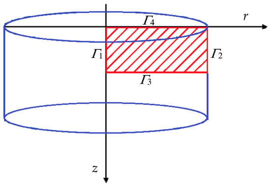
Figure 1.
Modeled sample with considered domain and boundary.
Internal fuzzy heat source is a sum of sources connected with perfusion of blood flow, metabolic heat production, and the absorption of heat from external sources:
where particular fuzzy summation terms [W·m−3] are the heat sources connected with perfusion, metabolism, and laser irradiation or the heat source generated by MNPs under an applied magnetic field, respectively.
The first analyzed external heat source was the fuzzy laser heat source described using Beer’s law [4]:
where [W·m−2] is the fuzzy surface irradiance of the laser, rB [m] is the radius of a laser beam, and s(t) is the function that equals 1 when the laser is on and equals 0 when the laser is off, whereas [m−1] denotes the fuzzy attenuation coefficient defined as follows [20]:
where [m−1] is the fuzzy absorption coefficient and [m−1] is the fuzzy effective scattering coefficient, which may be treated either as a constant value or as a function of the injury Arrhenius integral:
The fuzzy Arrhenius integral of the injury due to [19] is defined as follows:
where A [s−1] is the pre-exponential factor, [J·mole−1] is the activation energy of the reaction, and R [J·mole−1·K−1] is a universal gas constant (the values of parameters can be seen in Table 1).

Table 1.
Arrhenius injury integral parameters [21].
The fuzzy perfusion heat source function is considered as follows:
where [m3blood·s−1·m−3tissue] is the fuzzy blood perfusion rate, [J·m−3·K−1] is the fuzzy volumetric specific heat of blood, and TB [°C] denotes the artery temperature. Furthermore, the perfusion rate is represented as a function that accounts for necrotic changes taking place in the tissue [19]:
where represents the fuzzy initial perfusion rate, and we assume that function w follows a fuzzy polynomial form [19]:
where mj are fixed single-valued coefficients (see Table 2).

Table 2.
The coefficients of the perfusion coefficient function [21].
The second fuzzy external heat source under analysis was generated by MNPs under an applied magnetic field [22]:
where [s] means the effective relaxation time of nanoparticles, is the equilibrium susceptibility, [H·m−1] is the permeability, [A2·m−2] is the magnitude, and [Hz] is the frequency of an alternating magnetic field. Moreover, the volume fraction φ can be written as a function of the density of nanoparticles ρMNP [kg·m−3] and the volume concentration of ferrofluid as follows [22]:
where = 170 [mg·mL−1] is the maximum concentration of nanofluid at the injection site after injection, and parameter d0 determines the MNP diffusion distance from the injection site.
Equation (2) additionally necessitates the definition of boundary and initial conditions to fully establish the problem. The considered model incorporates boundary conditions of the following types [22]:
whereas on the irradiated surface, the third type of boundary condition is considered as follows [22]:
where n0 [m] is an external normal vector (n0 = [nx, ny]). The initial temperature distribution is considered to be constant T0 [°C].
To determine the temperature distribution, the fuzzy Pennes equation is solved numerically. In this work, the Fuzzy Finite Pointset Method (FPM) is employed for that purpose, with its detailed description provided in Section 2.
2. The Fuzzy Finite Pointset Method
The Finite Pointset Method (FPM) is a meshless Lagrangian approach that employs weighted least-squares interpolation to approximate spatial derivatives and address partial differential equations [23]. The method makes use of Taylor series expansions to evaluate function values and their derivatives, where the unknown coefficients of the expansion represent these quantities. Comprehensive descriptions and classical applications of FPM can be found in the literature [23,24,25,26].
In this section, we introduce the fundamental concepts of the fuzzy extension of FPM, developed to allow the method to be applied to mathematical models that incorporate uncertainties. When input parameters are expressed as fuzzy values, the resulting temperature is also represented as a fuzzy number. At the same time, those portions of the matrices that do not contain fuzzy terms remain crisp (i.e., single-valued). Vectors involving fuzzy quantities are marked with a tilde. The method is demonstrated here in the context of the Pennes equation expressed in cylindrical coordinates.
Consider a domain X with a prescribed boundary, containing n points x1, x2, …, xn (xj = [xj1, xj2], j = 1 … n), each associated with respective function values (x1,t), (x2,t), …, (xn,t). The objective is to approximate the value of at a chosen location x (x = [x1, x2]) and time moment t. To achieve this, we define the approximation of using a Taylor series expansion (dxjk = xjk − xk, k = 1,2) centered around x:
The values that are not known obtained by using the weighted least-squares method, in which the quadratic expression is minimized across all neighboring points (see subindex—np):
where weight coefficients and
where is a positive constant. The value h is a radius that defines a set of neighbor points around x [7,11].
If the point x is located within the interior of the X domain, the matrix M, incorporating the Pennes Equation (2) at the last row (where Δt denotes the time step) that must be satisfied by these interior points, is defined as follows [7,11]:
Then, and take the following form ( is a time counter) [7,11]:
Equation (16) can be expressed in the following form:
where
Formally, the minimization of the function J results in the following:
Additionally, FPM functions as an iterative method, where the vector is recalculated for each particle using the formula (23). It is worth mentioning that part , after multiplication, yields a matrix with single-valued entries. Multiplying such a matrix by a fuzzy vector, i.e., a vector containing a sequence of fuzzy numbers, does not require the use of any special fuzzy computational methods. Each value of the vector is multiplied by the corresponding matrix element and, in accordance with matrix algebra, summed up.
The algorithm applied includes a stopping criterion based on a relative error calculated for the lower and upper bounds of the fuzzy temperature intervals corresponding to the α-cut at α = 0, with the following structure:
where is the iteration counter, and is the maximum relative error.
Furthermore, if the point x lies on the boundary of X and meets the second type of boundary condition, an additional row must be included in matrix (18), and one additional element in vector (15), , because we have one equation more. And then for the third boundary condition, we have and , respectively.
In the proposed numerical method, triangular fuzzy numbers were employed, characterized by a set defined through the following membership function [14]:
where is the core of the number, are the left and the right end of the number, respectively. A triangular fuzzy number can be written as .
Those parameters of tissue that were assumed as symmetrical triangular fuzzy numbers are in the following form:
where p denotes the exact value of the parameter and u defines the width of the fuzzy number (u% = 0.01u).
A triangular fuzzy number can be represented through its α-cuts, each defined as a closed interval of the following form:
To solve the problem under consideration, closed intervals and directed interval arithmetic were employed. The use of α-cuts facilitates this process by enabling the decomposition of fuzzy numbers into a family of crisp intervals, which significantly simplifies the execution of mathematical operations within the fuzzy framework.
3. Results and Discussion
This study concludes by presenting the results obtained from the numerical simulations. Two numerical examples, each based on different sets of input data, are introduced. To evaluate the effectiveness of the proposed computational method, the results from the first example are compared with benchmark numerical data reported in [21].
The first example is analyzed using the parameters listed in Table 1. In this numerical example, the Pennes equation is examined with parameters such as perfusion rate and effective scattering coefficient, both of which are affected by tissue damage. The considered domain measures 15 × 12 mm. The model is improved by implementing a third-type boundary condition on the tissue surface exposed to laser irradiation, while adiabatic boundary conditions are applied to the other surfaces [21]. For the third-kind boundary condition, the following input values are used: α = 10 W·m−2·K−1 (convective heat transfer coefficient) and Tamb = 20 °C (ambient temperature). The stopping criterion defined in Equation (24) was set to ε = 10−4.
The initial temperature across the entire domain is uniformly set to T0 = 37 °C. The maximum laser intensity is assumed to be I0 = 30 kW·m−2. The tissue’s thermo-optical properties are listed in Table 3, while the parameters for the Arrhenius injury integral are given in Table 1. The coefficients for the function (10) are presented in Table 2. It should be noted that the optical properties used here are typical for near-infrared radiation interacting with soft tissue, such as the emission from a Nd:YAG laser at 1064 nm. In this context, during laser-induced coagulation, the reduced scattering coefficient may increase by a factor of 3–4 relative to its baseline value in native tissue, whereas the absorption coefficient remains unchanged [19].

Table 3.
Thermo-optical parameters [21].
Input parameters, including the initial blood perfusion coefficient, tissue absorption coefficient, effective scattering coefficients of native and damaged tissue, metabolic heat source, and peak power intensity, were modeled as fuzzy numbers (see Equation (26)). In the computations, u was set to 5.
Numerical simulations were performed at three specific depths: 0 mm, 1 mm, and 1.5 mm, along the main optical axis of the laser beam (Figure 2). The results obtained using the fuzzy version of FPM (black lines for α = 0) show very good agreement with the classical single-valued FPM solution (red lines), as detailed in [21]. Figure 3a presents the temperature profiles corresponding to various α-cuts. The red line represents the α-cuts for α = 1, which closely match the single-valued results.
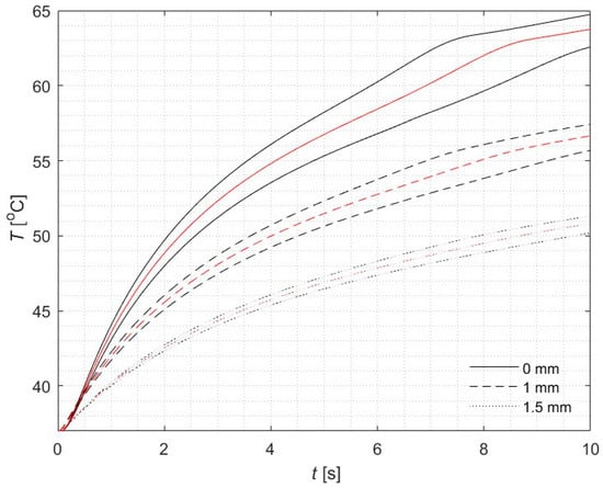
Figure 2.
Courses of fuzzy for α = 0 (black) and reference (red) temperature in three different points of the domain for z = 0, 1, 1.5 mm (r = 0).
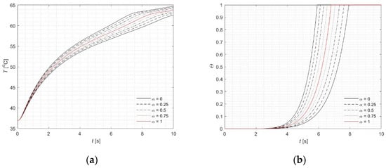
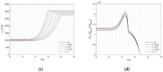
Figure 3.
Courses of (a) fuzzy temperature, (b) the fuzzy injury integral, (c) the fuzzy effective scattering coefficient, (d) the fuzzy perfusion coefficient for tissue surface (z = 0) and r = 0.
As illustrated in Figure 3b, the injury integral reaches 1—signifying complete tissue necrosis—between 5.91 s and 7.9 s, with the precise single-valued result being 6.8 s. This interval also corresponds to the point in Figure 3c where the effective scattering coefficient begins to level off. Similar behavior is observed in the computations using a fuzzy blood perfusion coefficient (Figure 3d). Together, these figures (Figure 3b–d) clearly highlight both the correlation and the influence of the injury integral on the associated parameters.
Calculations were also carried out for three different values of the parameter u to examine its influence on the results (Figure 4). The selection of this parameter is crucial for the analysis and depends on the spread of various input parameters in the mathematical model. It is evident from the plot that the lines are not evenly spaced, which results from the strongly nonlinear nature of the analyzed phenomenon. For clarity of comparison, the results were plotted for the extreme values of the fuzzy numbers, i.e., for α = 0. A detailed comparison of interval widths for α = 0 is presented in Table 4, along with the calculated width relative to the corresponding reference temperature value. The greater the value of u, the wider the temperature interval becomes, which is expected. However, as the computation time progresses, although the intervals would naturally be expected to widen, this tendency is disrupted due to the nonlinearity of the problem.
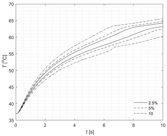
Figure 4.
Courses of fuzzy temperature for tissue surface (z = 0) and r = 0 for three values of u (2.5, 5, and 10) and α = 0.

Table 4.
Comparison of the fuzzy temperature widths at selected time moments for different values of u and for α = 0.
The second example demonstrates an application of the external heat source generated by MNPs under an applied magnetic field. The solute of nanofluid in this study is assumed to be Fe3O4 particles with a nanometer radius of 7 nm, subjected to a magnetic field (Table 5). Magnitude of a magnetic field Hm is assumed due to the formula for B = 0.03 T [27]. The considered domain, measuring 15 × 20 mm, was divided into two layers with thicknesses of 5 mm (outer layer, denoted as 1) and 10 mm (inner layer, denoted as 2). Furthermore, it was assumed that the outer layer represents tumor tissue, while the inner one corresponds to healthy tissue. The parameters used in the numerical analysis of both layers are listed in Table 6. In the model, a third-type boundary condition on the tumor tissue surface is implemented, while adiabatic boundary conditions are applied to the other surfaces [22]. For the third-kind boundary condition, the following input values are used: α = 4.2 W·m−2·K−1 and Tamb = 25 °C. The stopping criterion defined in Equation (24) was set to ε = 10−4. Location of the point of the highest concentration of nanoparticles (r0, z0) is set to (0, 2.5) mm and value d0 = 2 mm in (12). The initial temperature throughout the entire domain is set uniformly at T0 = 37 °C. In the formula (11), the fuzzy equilibrium susceptibility is treated as temperature dependent [28]:
where V [m3] is the volume of a single nanoparticle and [J·K−1] is the Boltzmann constant and [A·m−1] is the fuzzy saturation magnetization of the magnetic nanoparticles [29]:
where is the saturation magnetization at temperature 0 K and is the Curie temperature.

Table 5.
Properties of Fe3O4 and magnetic field [22,29].

Table 6.
Material properties of blood, tumor, and healthy tissue [22,30].
Input parameters like initial blood perfusion coefficient, metabolic heat source, and the effective relaxation time of nanoparticles were treated as fuzzy numbers (see Formula (26)). In the calculations, u is assumed to be 5 or 10. Numerical calculations were carried out at three specified depths, 0 mm, 1 mm, and 2.5 mm, located along the primary optical axis of the laser beam (Figure 5). The results obtained using the fuzzy version of the FPM (black lines for α = 0) and the classical version (red lines) show very good agreement with those reported in detail in [22]. This agreement indicates that the fuzzy extension preserves the main physical behavior of the system while capturing the uncertainty in input parameters.
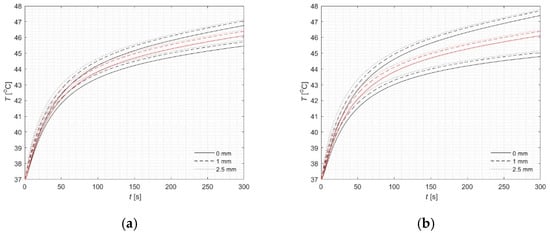
Figure 5.
Courses of fuzzy temperature for three chosen points (classical version—red lines) for r = 0: (a) 5%, (b) 10%.
The rest of the analysis is concentrated at the point (0, 2.5) mm, where the maximum concentration of MNPs is located, resulting in the highest temperature rise (Figure 6, Figure 7 and Figure 8). This observation can be physically explained by the fact that the local concentration of nanoparticles directly affects the absorption of energy from the alternating magnetic field, leading to localized heating. Individual lines in the plots correspond to specific α-cut levels. Simulations were conducted for u = 5 and u = 10 in order to illustrate the substantial influence of this parameter on the results. The observed temperature differences highlight the sensitivity of the heating process to the choice of u, emphasizing the need for proper calibration to accurately predict tissue response. Figure 6 presents the profiles of the fuzzy temperature, while a detailed analysis of the interval ranges defined by the α-cuts is provided in Table 7. Additionally, results of computations were presented for the fuzzy Arrhenius integral (Figure 7) and the fuzzy source term Q (Figure 8). These analyses reveal how uncertainty in the parameters not only affects the instantaneous temperature but also the cumulative thermal damage and source term distribution, which are critical for predicting tissue response during therapy. The magnitude of input parameter fuzziness in numerical analysis is typically selected based on the expected level of uncertainty associated with experimental measurements, material properties, or boundary conditions. This uncertainty can stem from variability in biological tissue characteristics, limitations in measurement precision, or natural fluctuations in environmental conditions. In practice, the fuzzy spread (e.g., the width of the triangular fuzzy number) is defined using expert knowledge, statistical data, or past sensitivity studies. The aim is to capture realistic variability without introducing excessive computational burden. Therefore, a balance must be struck between representing input uncertainty accurately and maintaining numerical stability and efficiency.
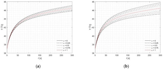
Figure 6.
Courses of fuzzy temperature (classical version—red lines) for point (0, 2.5) mm: (a) 5%, (b) 10%.
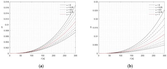
Figure 7.
Courses of fuzzy Arrhenius integral (classical version—red lines) for point (0, 2.5) mm: (a) 5%, (b) 10%.
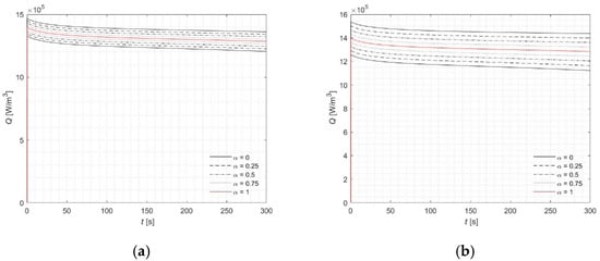
Figure 8.
Courses of fuzzy source term Q (classical version—red lines) for point (0, 2.5) mm: (a) 5%, (b) 10%.

Table 7.
Comparison of the fuzzy temperature widths at selected time moments for different values of u and α.
4. Conclusions
A novel fuzzy FPM approach in cylindrical coordinates for the analysis of transient bioheat transfer problems has been presented in this article. For the assessment of this extended numerical technique, the considered bioheat transfer problems were modeled by the Pennes equation in cylindrical coordinates. In addition to laser-induced heating, the analysis included a fuzzy modeling of magnetic nanoparticle-based heating, which yielded results in good agreement with corresponding reference solutions reported in [22]. The easy and effective incorporation of boundary conditions remains a key feature, enhancing its computational implementation also in 3D scenarios. Notably, all simulations were carried out using original in-house codes written in MATLAB R2025a, allowing the flexible application of various fuzzy numbers. In this work, triangular fuzzy numbers were used together with the α-cut technique, enabling effective modeling of input parameter uncertainty.
Instead of performing a classical sensitivity analysis—which is often computationally expensive and complex due to the need to evaluate the influence of multiple parameters on the output—fuzzy number computations offer an efficient alternative. Sensitivity analysis is typically performed to understand how variations in model inputs affect the results, which is particularly important when dealing with uncertain or imprecise data. The fuzzy approach implicitly captures this variability by allowing uncertain parameters to be represented as fuzzy numbers, eliminating the need for repeated simulations over a wide parameter space [31].
Due to the good numerical behavior, the efficient and stable performance of the method, and its ability to handle uncertainty, it can be concluded that this novel fuzzy approach is a promising computational tool for modeling nonlinear dynamic thermal processes in biological tissues subjected to laser irradiation and magnetic nanoparticle heating, and it is well-suited for future extensions using other bioheat equations such as the Cattaneo–Vernotte equation [32] or the dual-phase lag equation [33].
Funding
This research was funded by financial resources from the statutory subsidy of the Faculty of Mechanical Engineering, Silesian University of Technology (2025).
Institutional Review Board Statement
Not applicable.
Informed Consent Statement
Not applicable.
Data Availability Statement
The original contributions presented in this study are included in the article. Further inquiries can be directed to the author.
Conflicts of Interest
The author declares no conflicts of interest.
References
- Korczak, A. Numerical modeling of tissue laser irradiation with uncertain parameters using the interval finite pointset method. J. Appl. Math. Comput. Mech. 2024, 23, 41–53. [Google Scholar] [CrossRef]
- Korczak, A. Application of the fuzzy finite pointset method to the numerical modeling of tissue laser irradiation. In Proceedings of the 2024 IEEE International Conference on Fuzzy Systems (FUZZ-IEEE 2024), Yokohama, Japan, 30 June–5 July 2024; pp. 1–6. [Google Scholar] [CrossRef]
- Korczak, A.; Saucedo-Zendejo, F.R. Application of the Finite Pointset Method to the numerical modeling of heat transfer in a two-dimensional tissue subjected to a moving laser beam. Comput. Assist. Methods Eng. Sci. 2025; in press. [Google Scholar] [CrossRef]
- Glenn, T.N.; Rastegar, S.; Jacques, S.L. Finite element analysis of temperature controlled coagulation in laser irradiated tissue. IEEE Trans. Biomed. Eng. 1996, 43, 79–88. [Google Scholar] [CrossRef]
- Salloum, M.; Ma, R.H.; Weeks, D.; Zhu, L. Controlling nanoparticle delivery in magnetic nanoparticle hyperthermia for cancer treatment: Experimental study in agarose gel. Int. J. Hyperth. 2008, 24, 337–345. [Google Scholar] [CrossRef]
- Singh, M.; Ma, R.; Zhu, L. Quantitative evaluation of effects of coupled temperature elevation, thermal damage, and enlarged porosity on nanoparticle migration in tumors during magnetic nanoparticle hyperthermia. Int. Commun. Heat Mass Transf. 2021, 126, 105393. [Google Scholar] [CrossRef]
- Kuhnert, J. General Smoothed Particle Hydrodynamics. Ph.D. Thesis, Technische Universität Kaiserslautern, Kaiserslautern, Germany, 1999. [Google Scholar]
- Tiwari, S.; Klar, A.; Russo, G. Modelling and simulations of moving droplet in a rarefied gas. Int. J. Comput. Fluid Dyn. 2021, 35, 666–684. [Google Scholar] [CrossRef]
- Drumm, C.; Tiwari, S.; Kuhnert, J.; Bart, H.J. Finite pointset method for simulation of the liquid-liquid flow field in an extractor. Comput. Chem. Eng. 2008, 32, 2946–2957. [Google Scholar] [CrossRef]
- Saucedo-Zendejo, F.R.; Nóbrega, J.M. A novel approach to model the flow of generalized Newtonian fluids with the finite pointset method. Comput. Part. Mech. 2022, 9, 585–595. [Google Scholar] [CrossRef]
- Reséndiz-Flores, E.O.; Saucedo-Zendejo, F.R. Two-dimensional numerical simulation of heat transfer with moving heat source in welding using the finite pointset method. Int. J. Heat Mass Transf. 2015, 90, 239–245. [Google Scholar] [CrossRef]
- Saucedo-Zendejo, F.R. A novel meshfree approach based on the finite pointset method for linear elasticity problems. Eng. Anal. Bound. Elem. 2022, 136, 172–185. [Google Scholar] [CrossRef]
- Saucedo-Zendejo, F.R.; Medrano-Mendieta, J.L.; Nuñez-Briones, A.G. A GFDM approach based on the finite pointset method for two-dimensional piezoelectric problems. Eng. Anal. Bound. Elem. 2024, 163, 12–22. [Google Scholar] [CrossRef]
- Doss, L.J.T.; Kousalya, N. Finite pointset method for biharmonic equations. Comput. Math. Appl. 2008, 75, 3756–3785. [Google Scholar] [CrossRef]
- Piasecka-Belkhayat, A.; Korczak, A. Numerical modelling of transient heat transport in a two-layered metal film using the fuzzy lattice Boltzmann method with α-cuts. AIP Conf. Proc. 2018, 1922, 060005. [Google Scholar] [CrossRef]
- Skorupa, A.; Piasecka-Belkhayat, A. Application of fuzzy finite difference method in heat and mass transfer during cryopreservation process. Recent Adv. Comput. Oncol. Pers. Med. 2021, 1, 56–66. [Google Scholar]
- Delgato, Y.Z.; Wasques, V.F. A study of the heat transfer in materials with interval and fuzzy values via extension principle. Comput. Appl. Math. 2022, 41, 343. [Google Scholar] [CrossRef]
- Korczak, A.; Jasiński, M. Modelling of biological tissue damage process with application of interval arithmetic. J. Theor. Appl. Mech. 2019, 57, 249–261. [Google Scholar] [CrossRef]
- Abraham, J.P.; Sparrow, E.M. A thermal-ablation bioheat model including liquid-to-vapor phase change, pressure- and necrosis-dependent perfusion, and moisture-dependent properties. Int. J. Heat Mass Transf. 2007, 50, 2537–2544. [Google Scholar] [CrossRef]
- Niemz, M.H. Laser–Tissue Interaction, 3rd ed.; Springer-Verlag: Berlin/Heidelberg, Germany, 2007. [Google Scholar] [CrossRef]
- Jasiński, M. Modelling of thermal damage in laser irradiated tissue. J. Appl. Math. Comput. Mech. 2015, 14, 67–78. [Google Scholar] [CrossRef][Green Version]
- Tang, Y.; Wang, Y.; Flesch, R.C.C.; Jin, T. Influence of different heat transfer models on therapeutic temperature prediction and heat-induced damage during magnetic hyperthermia. J. Therm. Biol. 2023, 118, 103747. [Google Scholar] [CrossRef] [PubMed]
- Kuhnert, J.; Tiwari, S. Grid Free Method for Solving the Poisson Equation; Berichte des Fraunhofer-Instituts für Techno- und Wirtschaftsmathematik (ITWM Report); Fraunhofer-Institut für Techno- und Wirtschaftsmathematik: Kaiserslautern, Germany, 2001; Volume 25, Available online: https://publica-rest.fraunhofer.de/server/api/core/bitstreams/3e6a74bc-abf6-417f-ab5d-16b3a624c76c/content (accessed on 2 September 2025).
- Saucedo-Zendejo, F.R.; Reséndiz-Flores, E.O. Meshfree numerical approach based on the finite pointset method for two-way coupled transient linear thermoelasticity. Comput. Part. Mech. 2023, 10, 289–302. [Google Scholar] [CrossRef]
- Wawreńczuk, A.; Kuhnert, J.; Siedow, N. FPM computations of glass cooling with radiation. Comput. Methods Appl. Mech. Eng. 2007, 196, 4656–4671. [Google Scholar] [CrossRef]
- Saucedo-Zendejo, F.R.; Reséndiz-Flores, E.O. Meshfree numerical approach based on the finite pointset method for static linear elasticity problems. Comput. Methods Appl. Mech. Eng. 2020, 372, 113367. [Google Scholar] [CrossRef]
- Rosensweig, R.E. Heating magnetic fluid with alternating magnetic field. J. Magn. Magn. Mater. 2002, 252, 370–374. [Google Scholar] [CrossRef]
- Carrey, J.; Mehdaoui, B.; Respaud, M. Simple models for dynamic hysteresis loop calculations: Application to hyperthermia optimization. J. Appl. Phys. 2011, 109, 083921. [Google Scholar] [CrossRef]
- Cullity, B.D.; Graham, C.D. Introduction to Magnetic Materials, 2nd ed.; Wiley-IEEE Press: Hoboken, NJ, USA, 2008. [Google Scholar] [CrossRef]
- Tang, Y.; Zou, J.; Flesch, R.C.C.; Jin, T. Effect of injection strategy for nanofluid transport on thermal damage behavior inside biological tissue during magnetic hyperthermia. Int. Commun. Heat Mass Transf. 2022, 133, 105979. [Google Scholar] [CrossRef]
- Piasecka-Belkhayat, A.; Korczak, A. Modelling of thermal processes in 1D domain of crystalline solids using the lattice Boltzmann method. J. Theor. Appl. Mech. 2017, 55, 167–175. [Google Scholar] [CrossRef][Green Version]
- Majchrzak, E.; Kałuża, G.; Poteralska, J. Application of the DRBEM for numerical solution of Cattaneo–Vernotte bioheat transfer equation. Sci. Res. Inst. Math. Comput. Sci. 2008, 7, 11–12. [Google Scholar][Green Version]
- Partovi, B.; Ahmadikia, H.; Mosharaf-Dehkordi, M. Analytical and numerical analysis of the dual-pulse lag heat transfer in a three-dimensional tissue subjected to a moving multi-point laser beam. J. Therm. Biol. 2023, 112, 103431. [Google Scholar] [CrossRef]
Disclaimer/Publisher’s Note: The statements, opinions and data contained in all publications are solely those of the individual author(s) and contributor(s) and not of MDPI and/or the editor(s). MDPI and/or the editor(s) disclaim responsibility for any injury to people or property resulting from any ideas, methods, instructions or products referred to in the content. |
© 2025 by the author. Licensee MDPI, Basel, Switzerland. This article is an open access article distributed under the terms and conditions of the Creative Commons Attribution (CC BY) license (https://creativecommons.org/licenses/by/4.0/).