Domain-Oriented Hierarchical Topology Optimisation—An Approach for Heterogeneous Materials ^†

Abstract

In structural topology optimisation, intermediate densities are typically interpreted as local distributions of heterogeneous materials, bridging the gap between a solid and a void through optimised arrangements of cellular or composite microstructures. These multiscale configurations, governed by interactions between micro- and macroscales, are commonly addressed via hierarchical approaches. However, such methods often suffer from high computational cost and limited practical applicability. This work proposes an alternative strategy that reformulates the hierarchical problem by replacing pointwise microscale variations with a subdomain-based formulation. Each subdomain is associated with a periodic microstructure, reducing the number of local problems and significantly decreasing computational demands. A multiscale topology optimisation framework is developed using Asymptotic Expansion Homogenisation, enabling effective macrostructural properties and supporting inverse homogenisation for microscale design. The proposed method is implemented in a user-developed code and validated through several benchmark problems. The results show that the subdomain approach yields discrete and manufacturable microstructures that better reflect real-world composite applications, while also achieving substantial improvements in computational efficiency.

1. Introduction

Structural topology optimisation consists essentially of searching for the optimal material distribution within a given structure. This distribution, usually defined by material density variables, ranges between high and low density regions. A common way of relaxing the original discrete problem, where there are only the limit values of dense material and a void, is by allowing the use of intermediate density values. The physical sense of this option comes from the use of local microstructures, filling the gap between dense material and a void with different optimal distributions of cellular or composite materials. This process is performed at least on two size scales. This is sometimes called the homogenisation approach and has been presented according to different methods and implementations for solving the local problem [1,2,3,4,5,6,7,8,9,10,11]. It pushes the discrete material distribution to the microscale, making the macrostructure density values smooth, homogenised reflections of the local material distribution. The general method of addressing the two-scale problem is called multilevel or hierarchical [4,6,8,12,13,14,15]. This tends to lead, moreover, in a free material approach as the one used in this work, not only to high-cost computations but also to a limited application range for the effective fabrication of optimal structures. In this sense, this work shows a different approach. Instead of a hierarchical problem with pointwise local topology variation, this is performed over subdomains of the global structure. This allows the size of the problem to become much more manageable. Furthermore, this brings the hierarchical methodologies closer to a point where the solutions are feasible and more in sync with the practical applications of composite materials.

The authors use an in-house developed code [16,17], capable of several types of calculation and a broad range of topology optimisation configurations. This paper is centred on the evaluation of the subdomain approach. The multiscale methods presented can hence be divided in the following ways: simultaneous optimisation of structure and material in a full hierarchical strategy; multiscale optimisation focused on the optimal microscale for a given structure (one domain); and multiple macroscale subdomain multiscale optimisation. These alternative strategies are illustrated in Figure 1. The developed code [16] was implemented with alternative optimisation algorithms, using optimality criteria methods, several variations of the Method of Moving Asymptotes (MMA) [18] and CONLIN [19,20]. In this work, the focus is on the MMA algorithm, since it is one of the most widely used and most efficient methods in these applications.

Compared to hierarchical formulations that require a local problem per finite element, the proposed subdomain strategy reduces the number of microscale problems to the number of predefined subdomains. This leads to significantly lower computational cost while maintaining the coupling between scales. Furthermore, the subdomain approach allows engineers to align numerical regions with structural functions, making it more compatible with practical composite design and manufacturing constraints.

2. Hierarchical Formulation in Linear Elasticity

The initial definition of the topology optimisation problem is discrete, where the material used in the finite elements is considered to be the prescribed material or a void, controlled by a binary variable. Most solutions, however, use some kind of relaxed version of the problem, where the material properties can vary continuously between full material and a void. One method defines a continuous pseudo-density variable, $\rho$, which can take values between 0 and 1. In this case material properties, K, for a given element become

$$\begin{array}{c}\hfill K\left(\rho \right)={\rho }^p{K}_0,\end{array}$$

(1)

where $K_0$ is the base material property. p is a penalisation value used to penalise intermediate densities, numerically trying to direct the solution to a discrete distribution [9,21]. This is a popular method called SIMP (Solid Isotropic Material with Penalisation) [22,23]. The stiffness of a finite element e is defined by ${\rho }_e^p{\mathbf{k}}_0$, where ${\mathbf{k}}_0$ is the element stiffness matrix when element e is built from the base material. This is the same as using ${\rho }_e^p{\mathbf{D}}_0$, where ${\mathbf{D}}_0$ is the elasticity constitutive matrix of the base material. ${\rho }_{\min }$ is a lower limit for the density variable, used to avoid system singularities arising from elements with no stiffness. Note that there are several alternatives to the traditional SIMP approach [23,24]. One of those comes from changing the power law to

$$\begin{array}{c}\hfill K\left(\rho \right)={\rho }^p{K}_1+(1-{\rho }^p)K_2,\end{array}$$

(2)

which allows the use of two materials, 1 and 2, instead of material and a void, with $K_1>K_2$. This makes sense when using a composite instead of cellular materials. It also allows the use of material and a void, but puts the control of the minimum stiffness and conditioning of the system on the minimum value chosen for $K_2$ instead of the density variable. In either case, this power law can be used as

$$\begin{array}{ccc}\hfill K\left(\rho \right)& =& {\rho }^p{K}_0+(1-{\rho }^p){\mathrm{d}}_m{K}_0\hfill \\ & =& \left[{\rho }^p+{\mathrm{d}}_m(1-{\rho }^p)\right]K_0,\hfill \end{array}$$

(3)

where $d_{\mathrm{m}}={\displaystyle \frac{K_{\min }}{K_0}}$. $K_{\min }$ is the minimum value for property K, used to define the softer material phase or for void conditioning. This is the method used in this work, with $d_{\mathrm{m}}=0$ for the SIMP definition and $d_{\mathrm{m}}\ne 0$ for different conditioning control strategies and composite material processing. Another approach with the same practical implications is the modified SIMP method [24], defined as

$$\begin{array}{c}\hfill K\left(\rho \right)=K_{\min }+{\rho }^p(K_0-K_{\min }).\end{array}$$

(4)

$K_{\min }\ne 0$ to avoid singularities and conditioning problems. These alternative forms have some advantages over the usual SIMP definition, namely on the fact that the minimum value for K becomes independent from the penalty value and that they are more compatible with a wider variety of filtering techniques [24].

The objective of structural optimisation is usually compliance minimisation (or stiffness maximisation) of a structure. The widely used form in linear elasticity is compliance minimisation, using as a measure the scalar defining the strain energy,

$$\begin{array}{c}\hfill S={\displaystyle \frac{1}{2}}{\int }_{\mathrm{\Omega }}{\rho }^p\mathit{\epsilon }\left(\mathbf{u}\right):{\mathbf{D}}^0:\mathit{\epsilon }\left(\mathbf{u}\right)\mathrm{d}\mathrm{\Omega },\end{array}$$

(5)

where $\rho =\rho \left(\mathbf{x}\right)$ is the macrostructural density value, or using the work of external loads as

$$\begin{array}{c}\hfill W={\int }_{\mathrm{\Omega }}\mathbf{b}·\mathbf{u}\mathrm{d}\mathrm{\Omega }+{\int }_{{\mathrm{\Gamma }}_{{\mathrm{N}}_{\mathrm{u}}}}\overline{\mathbf{t}}·\mathbf{u}\mathrm{d}\mathrm{\Gamma }.\end{array}$$

(6)

b and $\overline{\mathbf{t}}$ are the volume and surface loads, respectively. These energies can be used to define the total potential energy of the system as

$$\begin{array}{ccc}\hfill P=S-W& =& {\displaystyle \frac{1}{2}}{\int }_{\mathrm{\Omega }}{\rho }^p\mathit{\epsilon }\left(\mathbf{u}\right):{\mathbf{D}}^0:\mathit{\epsilon }\left(\mathbf{u}\right)\mathrm{d}\mathrm{\Omega }\hfill \\ & & -\left({\int }_{\mathrm{\Omega }}\mathbf{b}·\mathbf{u}\mathrm{d}\mathrm{\Omega }+{\int }_{{\mathrm{\Gamma }}_{{\mathrm{N}}_{\mathrm{u}}}}\overline{\mathbf{t}}·\mathbf{u}\mathrm{d}\mathrm{\Gamma }\right).\hfill \end{array}$$

(7)

According to the minimum total potential energy principle, the total potential energy is minimised by the displacement field u that defines the equilibrium state for the imposed boundary conditions. An advantage of using this energy definition as an objective function is that it explicitly shows the hierarchical multiscale structure of the problem [25]. In this sense, the hierarchical topology optimisation problem can be written as [4,6,8,9,26]

$$\begin{array}{c}\hfill \underset{\begin{array}{c}\rho \left(\mathbf{x}\right)\\ 0\le \rho \left(\mathbf{x}\right)\le 1\\ {\int }_{\mathrm{\Omega }}\rho \left(\mathbf{x}\right)\mathrm{d}\mathrm{\Omega }\le V\end{array}}{max}\underset{\begin{array}{c}\mathbf{u}\in U\end{array}}{min}\left[\phantom{\sum _{\mathrm{x}}}{\displaystyle \frac{1}{2}}{\int }_{\mathrm{\Omega }}\mathrm{\Phi }(\rho ,\mathbf{u})\mathrm{d}\mathrm{\Omega }\right.\\ \hfill \left.-\left({\int }_{\mathrm{\Omega }}\mathbf{b}·\mathbf{u}\mathrm{d}\mathrm{\Omega }+{\int }_{{\mathrm{\Gamma }}_{{\mathrm{N}}_{\mathrm{u}}}}\overline{\mathbf{t}}·\mathbf{u}\mathrm{d}\mathrm{\Gamma }\right)\right],\end{array}$$

(8)

where u is the equilibrium displacement field that minimises the potential energy. This is performed by solving the equilibrium finite element problem, which can be included as an additional constraint. x defines the quantities relative to the macroscale. The optimal energy density function $\mathrm{\Phi }(\rho ,\mathbf{u})$ is the solution for the local problem that can be defined as

$$\begin{array}{c}\hfill \mathrm{\Phi }(\rho ,\mathbf{u})=\underset{\begin{array}{c}\mu (\mathbf{x},\mathbf{y})\\ 0\le \mu (\mathbf{x},\mathbf{y})\le 1\\ {\int }_Y\mu (\mathbf{x},\mathbf{y})\mathrm{d}Y=\rho \left(\mathbf{x}\right)\end{array}}{max}\left[\phantom{{\displaystyle \frac{\mathrm{x}}{\mathrm{x}}}}{D}_{ijkl}^{\mathrm{h}}\left(\mu \right){\epsilon }_{ij}\left(\mathbf{u}\right){\epsilon }_{kl}\left(\mathbf{u}\right)\right],\end{array}$$

(9)

where y defines the quantities relative to the microscale. These problems lead to a coupled two-scale optimisation methodology—often referred to as a material distribution or local anisotropy problem. The dependence between both problems makes this non-linear in a constitutive definition, even if defined on a linear elastic basis [9]. The local problem results from a localisation process, where the local strain energy density is maximised according to the localised macrostructural strain. The two-scale problems are then clearly divided. In the macroscale problem the global structural finite element problem is solved, and the topology is described using a relaxed density variable $\rho \left(\mathbf{x}\right)$. While the usual approach is to force the limits for this variable using the SIMP penalised density, in this case, this variable is a measure of the corresponding local volume fraction. In each of the local problems, the localised macroscale information is used to solve the microscale topology optimisation problem using the local density variable $\mu (\mathbf{x},\mathbf{y})$. This is coupled to the macroscale density variable through the local volume constraints

$$\begin{array}{c}\hfill {\int }_{\mathrm{Y}}\mu (\mathbf{x},\mathit{y})\mathrm{d}Y=\rho \left(\mathbf{x}\right).\end{array}$$

(10)

Each of the local problems results in a given material distribution, in this case ideally discrete, according to the SIMP methodology. These distributions are evaluated using homogenisation methods to provide effective constitutive information to be used in the macroscale problem. The authors use the Asymptotic Expansion Homogenisation (HEA) method [27,28,29], but alternative formulations can be used with different homogenisation methods [3,4,5,6,7,10,23,30]. The homogenised elasticity constitutive matrix $D^{\mathrm{h}}$ is calculated with the base formulation of the HEA method. The main difference comes from the constituent microscale properties, which in this case are controlled by the base material and the SIMP penalised local densities $\mu$. Thus, the constitutive matrix $D_{e_{\mathrm{y}}}$ for an element $e_{\mathrm{y}}$ of the microscale can be defined as

$$\begin{array}{c}\hfill D_{e_{\mathrm{y}}}=D\left({\mu }_{e_{\mathrm{y}}}\right)={\mu }_{e_{\mathrm{y}}}^p{D}^0.\end{array}$$

(11)

In this sense, the homogenised tensor can be written as

$$\begin{array}{cc}& D_{ijmn}^{\mathrm{h}}={\displaystyle \frac{1}{\left|\mathrm{Y}\right|}}{\int }_{\mathrm{Y}}{D}_{ijkl}\left(\mu \right)\left({\mathrm{I}}_{kl}^{mn}-{\displaystyle \frac{\partial {\chi }_k^{mn}}{\partial y_l}}\right)\mathrm{d}Y,\hfill \end{array}$$

(12)

or, in the quadratic form (variational) [26], as

$$\begin{array}{ccc}& & D_{ijmn}^{\mathrm{h}}=\hfill \\ & & {\displaystyle \frac{1}{\left|\mathrm{Y}\right|}}{\int }_{\mathrm{Y}}{D}_{pqkl}\left(\mu \right)\left({\mathrm{I}}_{pq}^{ij}-{\displaystyle \frac{\partial {\chi }_p^{ij}}{\partial y_q}}\right)\left({\mathrm{I}}_{kl}^{mn}-{\displaystyle \frac{\partial {\chi }_k^{mn}}{\partial y_l}}\phantom{{\displaystyle \frac{\partial {\chi }_p^{ij}}{\partial y_q}}}\right)\mathrm{d}Y.\hfill \end{array}$$

(13)

$\chi$ is the tensor of displacement correctors and contains the eigendeformations of the representative periodic geometry. These changes to local properties, with the influence of the density interpolation, must also be used for the equations that define the local homogenisation problems [28]. In practical terms, these integrals represent how the microscale deformation field distributes strain energy, yielding effective stiffnesses that can be used at the macroscale. This ensures that the computed structural response reflects the anisotropy and heterogeneity of the designed microstructures.

Note that the hierarchical problem can also be written as

$$\begin{array}{c}\hfill \underset{\begin{array}{c}\rho \left(\mathbf{x}\right)\\ 0\le \rho \left(\mathbf{x}\right)\le 1\\ {\int }_{\mathrm{\Omega }}\rho \left(\mathbf{x}\right)\mathrm{d}\mathrm{\Omega }\le V\\ \mathbf{K}\mathbf{u}=\mathbf{f}\end{array}}{min}\left[{\displaystyle \frac{1}{2}}{\int }_{\mathrm{\Omega }}{D}_{ijkl}^{\mathrm{h}}\left(\mu \right){\epsilon }_{ij}\left(\mathbf{u}\right){\epsilon }_{kl}\left(\mathbf{u}\right)\mathrm{d}\mathrm{\Omega }\right],\end{array}$$

(14)

which uses as an objective function the minimisation of strain energy, equivalent, at the equilibrium, to the minimisation of the work of external loads (compliance). The definition of the necessary optimality conditions is well defined in the bibliography, using the augmented Lagrangian method [8]. In this paper, the optimality conditions will be presented for the subdomain problem.

3. Subdomain Multiscale Topology Optimisation

The hierarchical structure can be changed to make the topology optimisation domain-oriented. This changes the problem from a number of local optimisation problems equal to the number of macroscale finite elements to a predefined number of macroscale subdo- mains [26,31]. This follows a formulation similar to the one previously introduced. Consider that the macroscale domain $\mathrm{\Omega }$ is divided into a finite number of subdomains ${\mathrm{\Omega }}_q$, where $q=1,\dots ,Q$, such that $\mathrm{\Omega }={\cup }_{q=1}^Q{\mathrm{\Omega }}_q$ and ${\mathrm{\Omega }}_i\cap {\mathrm{\Omega }}_j=⌀,\forall i\ne j$. Each of these domains has constant material properties, corresponding to a periodical local microstructure. The optimisation problem becomes [26]

$$\begin{array}{ccc}& & \underset{\begin{array}{c}\rho \left(\mathbf{x}\right)\\ 0\le \rho \left(\mathbf{x}\right)\le 1\\ {\int }_{\mathrm{\Omega }}\rho \left(\mathbf{x}\right)\mathrm{d}\mathrm{\Omega }\le V\end{array}}{max}\underset{\begin{array}{c}\mathbf{u}\in U\end{array}}{min}\left[{\displaystyle \frac{1}{2}}\sum _{q=1}^Q{\overline{\mathrm{\Phi }}}_q(\rho ,\mathbf{u})\right.\hfill \\ & & \left.-\left({\int }_{\mathrm{\Omega }}\mathbf{b}·\mathbf{u}\mathrm{d}\mathrm{\Omega }+{\int }_{{\mathrm{\Gamma }}_{{\mathrm{N}}_{\mathrm{u}}}}\overline{\mathbf{t}}·\mathbf{u}\mathrm{d}\mathrm{\Gamma }\right)\right].\hfill \end{array}$$

(15)

This formulation differs from the hierarchical approach in that material properties are the same within each given domain q. The number of local problems is the same as the number of subdomains, Q. The optimal strain energy function ${\overline{\mathrm{\Phi }}}_q(\rho ,\mathbf{u})$ is the solution to the microscale problem for the subdomain ${\mathrm{\Omega }}_q$, written as

$$\begin{array}{ccc}& & {\overline{\mathrm{\Phi }}}_q(\rho ,\mathbf{u})=\hfill \\ & & \underset{\begin{array}{c}\mu (\mathbf{x},\mathbf{y})\\ 0\le \mu (\mathbf{x},\mathbf{y})\le 1\\ {\int }_Y\mu (\mathbf{x},\mathbf{y})\mathrm{d}Y=\rho \left(\mathbf{x}\right)\end{array}}{max}\left[D_{ijkl}^{\mathrm{h}}\left(\mu \right){\int }_{{\mathrm{\Omega }}_q}{\epsilon }_{ij}\left(\mathbf{u}\right){\epsilon }_{kl}\left(\mathbf{u}\right)\mathrm{d}\mathrm{\Omega }\right].\hfill \end{array}$$

(16)

The constitutive tensor ${\mathbf{D}}^{\mathrm{h}}$ is constant in ${\mathrm{\Omega }}_q$. This equation can be conveniently written as

$$\begin{array}{cc}& {\overline{\mathrm{\Phi }}}_q(\rho ,\mathbf{u})=\underset{\begin{array}{c}\mu (\mathbf{x},\mathbf{y})\\ 0\le \mu (\mathbf{x},\mathbf{y})\le 1\\ {\int }_Y\mu (\mathbf{x},\mathbf{y})\mathrm{d}Y=\rho \left(\mathbf{x}\right)\end{array}}{max}\left[D_{ijkl}^{\mathrm{h}}\left(\mu \right){\overline{S}}_{ijkl}\left(\mathbf{u}\right)\right],\hfill \end{array}$$

(17)

$$\begin{array}{ccc}& & {\overline{S}}_{ijkl}\left(\mathbf{u}\right)={\int }_{{\mathrm{\Omega }}_q}{\epsilon }_{ij}\left(\mathbf{u}\right){\epsilon }_{kl}\left(\mathbf{u}\right)\mathrm{d}\mathrm{\Omega }.\hfill \end{array}$$

(18)

$\overline{\mathbf{S}}$ [26] is the integration of the diadic products ${\epsilon }_{ij}\left(\mathbf{u}\right){\epsilon }_{kl}\left(\mathbf{u}\right)$ in ${\mathrm{\Omega }}_q$. As for the hierarchical problem, the subdomain problem can also be written as (vd. Equation (14))

$$\begin{array}{c}\hfill \underset{\begin{array}{c}\rho \left(\mathbf{x}\right)\\ 0\le \rho \left(\mathbf{x}\right)\le 1\\ {\int }_{\mathrm{\Omega }}\rho \left(\mathbf{x}\right)\mathrm{d}\mathrm{\Omega }\le V\\ \mathbf{K}\mathbf{u}=\mathbf{f}\end{array}}{min}\left[\phantom{\sum _{\mathrm{x}}}{\displaystyle \frac{1}{2}}\sum _{q=1}^Q{\overline{\mathrm{\Phi }}}_q(\rho ,\mathbf{u})\right],\end{array}$$

(19)

for the minimisation of the strain energy. In this case, this strategy provides the ability to include different averaging options for the operator ${\overline{\mathrm{S}}}_{ijkl}$. As will be shown in the results of this work, sometimes it is useful to unbalance the problem to avoid situations where the volume average kills the influence of important effects. In this case, the strain energy minimisation problem can be called an average strain energy minimisation problem. ${\overline{S}}_{ijkl}$ can in effect be defined in several different ways, using different averaging properties to numerically improve the convergence and overall behaviour of the problem, as

$$\begin{array}{c}\hfill {\overline{S}}_{ijkl}^{\prime }\left(\mathbf{u}\right)={\int }_{{\mathrm{\Omega }}_q}\iota {\epsilon }_{ij}\left(\mathbf{u}\right){\epsilon }_{kl}\left(\mathbf{u}\right)\mathrm{d}\mathrm{\Omega }.\end{array}$$

(20)

$\iota$ is a generic averaging parameter used to ponder the influence of each part of the desired effect or property, ${\iota }_{\mathrm{x}}$, with the corresponding total values, ${\iota }_{\mathrm{\Omega }}$, as $\iota ={\displaystyle \frac{{\iota }_{\mathrm{x}}}{{\iota }_{\mathrm{\Omega }}}}$. This allows more flexibility in how the effective behaviour of the structure influences the local behaviour. The choice of the weighting parameter $\iota$ should reflect the dominant mechanical response of interest. For example, volume averaging is suitable for low gradient stress fields, equivalent stress-based weighting better captures load-bearing regions under bending, and principal stress weighting is useful when specific orientations dominate the response. In practice, engineers may perform a preliminary structural analysis to identify which field (strain, stress, or principal direction) best represents the intended behaviour and choose the $\iota$ calculation mode accordingly.

Furthermore, note that an interesting aspect of this subdomain approach is that it can degenerate in two limit cases. On one hand, considering only one domain ($Q=1$) leads to a problem that is similar to an inverse homogenisation problem, where the optimisation is centred on only the microscale problem. The difference is that, where inverse homogenisation is used to prescribe macrostructural states, this evaluates the macrostructure response for each iteration of the local problem. On the other hand, if the number of domains is the same as the number of macroscale finite elements ($Q=n_{e_x}$), the numerical definition of the problem becomes equivalent to the hierarchical definition, with a local problem for each macroscale element.

Optimality necessary conditions can be obtained considering an augmented Lagrangian method similar to the one used for the hierarchical formulation [8],

$$\begin{array}{ccc}& & ℒ=\hfill \\ & & \underset{\begin{array}{c}u\in U\end{array}}{min}\left[{\displaystyle \frac{1}{2}}\sum _{q=1}^Q{\overline{\mathrm{\Phi }}}_q(\rho ,\mathbf{u})-\left({\int }_{\mathrm{\Omega }}\mathbf{b}·\mathbf{u}\mathrm{d}\mathrm{\Omega }+{\int }_{{\mathrm{\Gamma }}_{{\mathrm{N}}_{\mathrm{u}}}}\overline{\mathbf{t}}·\mathbf{u}\mathrm{d}\mathrm{\Gamma }\right)\right]\hfill \\ & & -{\displaystyle \frac{1}{2c}}\left\{{\left[max\left\{0,\mathrm{\Lambda }+c\left({\int }_{\mathrm{\Omega }}\rho \mathrm{d}\mathrm{\Omega }-V\right)\right\}\right]}^2-{\mathrm{\Lambda }}^2\right\},\hfill \end{array}$$

(21)

where c is the penalty parameter and $\mathrm{\Lambda }\ge 0$ is the Lagrange multiplier for the global volume constraint. Taking $\tilde{\mathbf{u}}$ as the equilibrium displacement field, the stationarity condition relative to the optimisation variable $\rho \left(\mathbf{x}\right)$ can be defined as

$$\begin{array}{ccc}& & {\displaystyle \frac{1}{2}}{\displaystyle \frac{\partial \overline{\mathrm{\Phi }}(\rho ,\tilde{\mathbf{u}})}{\partial \rho }}=\hfill \\ & & max\left[0,\mathrm{\Lambda }+c\left({\int }_{\mathrm{\Omega }}\rho \mathrm{d}\mathrm{\Omega }-V\right)\right],\forall \mathbf{x}\in \mathrm{\Omega },\hfill \end{array}$$

(22)

where $\rho \in ]0,1[$. For $\rho \in \{0,1\}$, this equality becomes an inequality condition (≤ when $\rho =0$ and ≥ when $\rho =1$) [8,25]. This is due to the fact that the conditions that limit the variable become active, and its Lagrange multipliers are different from zero. However, at these extremes, it is not needed to solve the local problems, since these are either the absence of material ($\mathbf{D}=0$) or dense material throughout ($\mathbf{D}={\mathbf{D}}^0$). The stationarity condition for the Lagrange multiplier leads to

$$\begin{array}{c}\hfill \mathrm{\Lambda }=max\left[0,\mathrm{\Lambda }+c\left({\int }_{\mathrm{\Omega }}\rho \mathrm{d}\mathrm{\Omega }-V\right)\right].\end{array}$$

(23)

Condition (23) forces the fulfilment of the global volume constraint. In turn, condition (22) shows the stability of the Lagrange multiplier $\mathrm{\Lambda }$ at the equilibrium and at the optimal solution, meaning that the derivative of the strain energy function in relation to the global densities is constant for any x (with $0<\rho <1$) [8,13].

The Lagrangian function for the local problem (Equation (17)) can be written as

$$\begin{array}{ccc}& & ℒ=\hfill \\ & & \left[D_{ijkl}^{\mathrm{h}}\left(\mu \right){\overline{S}}_{ijkl}\left(\tilde{\mathbf{u}}\right)\phantom{{\int }_{Y\left(\tilde{\mathbf{x}}\right)}}\right]-\lambda \left(\tilde{\mathbf{x}}\right)\left[{\int }_{Y\left(\tilde{\mathbf{x}}\right)}\mu \mathrm{d}\mathrm{y}-\rho \left(\tilde{\mathbf{x}}\right)\right].\hfill \end{array}$$

(24)

This Lagrangian is defined in each $\mathbf{x}\in \mathrm{\Omega }$, and the multiplier $\lambda$ is associated with the local volume constraint that connects the local density fields $\mu$ to the corresponding global density at each considered point of the macroscale or subdomain ($\rho \left(\mathbf{x}\right)$). ${\overline{S}}_{ijkl}\left(\tilde{\mathbf{u}}\right)$ are the components of $\overline{\mathbf{S}}$ for the displacements $\tilde{\mathbf{u}}$ at the equilibrium in $\tilde{\mathbf{x}}$. As for the global Lagrangian, the stationarity condition for the microstructural density variable $\mu$ can be defined as

$$\begin{array}{ccc}& & {\displaystyle \frac{\partial D_{ijkl}^{\mathrm{h}}\left(\mu \right)}{\partial \mu }}{\overline{S}}_{ijkl}\left(\tilde{\mathbf{u}}\right)=\lambda \left(\tilde{\mathbf{x}}\right),\hfill \\ & & \forall \mathbf{y}\in Y\left(\tilde{\mathbf{x}}\right),0<\mu <1,\hfill \end{array}$$

(25)

where

$$\begin{array}{ccc}\hfill {\displaystyle \frac{\partial D_{ijkl}^{\mathrm{h}}\left(\mu \right)}{\partial \mu }}& =& {\displaystyle \frac{1}{\left|Y\right|}}{\int }_{Y}p{\mu }^{p-1}{D}_{pqrs}^0\hfill \\ & & \times \left(\phantom{{\displaystyle \frac{\partial {\chi }_p^{ij}}{\partial y_q}}}{\delta }_{rk}{\delta }_{sl}-{\displaystyle \frac{\partial {\chi }_r^{kl}}{\partial y_s}}\right)\left({\delta }_{pi}{\delta }_{qj}-{\displaystyle \frac{\partial {\chi }_p^{ij}}{\partial y_q}}\right)\mathrm{d}Y\hfill \end{array}$$

(26)

are the sensitivities of the components of the homogenised elasticity tensor, $D^{\mathrm{h}}$, to the variation in $\mu$. As for the global problem, at the extremes, these conditions become inequalities because of the multipliers of the active boundary values for the variable limits. Condition (25) must be satisfied, for each x em $\mathrm{\Omega }$, in every y of the microscale representative unit-cell.

The Lagrangian defined in Equation (24) corresponds to the local problem defined by the objective function $\overline{\mathrm{\Phi }}(\rho ,\tilde{\mathbf{u}})$ (vd. Equation (16)) at the optimum. A stationarity condition in relation to the global density $\rho$, at the optimum $\tilde{\mathbf{x}}$, shows that

$$\begin{array}{c}\hfill {\displaystyle \frac{\partial \overline{\mathrm{\Phi }}(\rho ,\tilde{\mathbf{u}})}{\partial \rho }}=\lambda \left(\tilde{\mathbf{x}}\right),\forall \tilde{\mathbf{x}}\in \mathrm{\Omega }.\end{array}$$

(27)

Substituting in Equation (22),

$$\begin{array}{ccc}& & \lambda \left(\mathbf{x}\right)=2max\left[0,\mathrm{\Lambda }+c\left({\int }_{\mathrm{\Omega }}\rho \mathrm{d}\mathrm{\Omega }-V\right)\right],\hfill \\ & & \forall \mathbf{x}\in \mathrm{\Omega },0<\rho <1.\hfill \end{array}$$

(28)

Note that while $\lambda \left(\mathbf{x}\right)$ is a function, the second member of this equation is constant in $\mathrm{\Omega }$ ($0<\rho <1$) [25]. This means that at the optimum, the Lagrange multiplier for the local constraint will be constant in all macrostructural domains. Furthermore, condition (25) can be written as

$$\begin{array}{ccc}& & {\displaystyle \frac{\partial D_{ijkl}^{\mathrm{h}}\left(\mu \right)}{\partial \mu }}{\overline{S}}_{ijkl}\left(\tilde{\mathbf{u}}\right)=\lambda \left(\tilde{\mathbf{x}}\right)=2\mathrm{\Lambda },\hfill \\ & & \forall \mathbf{y}\in Y\left(\tilde{\mathbf{x}}\right),0<\mu <1,\hfill \end{array}$$

(29)

expressing the convergence dependence of both scales.

Note that the augmented Lagrangian method has as a main iteration for the dual problem, controlled by updating the Lagrange multipliers. In this sense, Equation (23) leads to [8]:

$$\begin{array}{c}\hfill {\mathrm{\Lambda }}_{t+1}=max\left[0,{\mathrm{\Lambda }}_t+c\left({\int }_{\mathrm{\Omega }}\rho \mathrm{d}\mathrm{\Omega }-V\right)\right].\end{array}$$

(30)

At the optimum point, ${\mathrm{\Lambda }}_{t+1}$ will be constant in all of the domain and equal to ${\mathrm{\Lambda }}_t$.

4. Numerical Modelling

Integrating homogenisation procedures in topology optimisation problems leads to a clear separation of the process into two parts: the optimisation and the homogenisation. While this may seem straightforward, it introduces several complexities. A homogenisation module serves the purpose of calculating effective properties for a heterogeneous medium. In a typical program this is performed once, at the beginning of the problem and stored to use in the global calculations. This is true for a finite element structural problem or for a macroscale topology optimisation problem with a prescribed microstructure. In the problems solved in this work, the homogenisation module is used to gather much more information, such as the local sensitivities for the variations in local densities. The artificial material distributions at the microscale require evaluation in each problem iteration, which in turn influences the overall structural behaviour and leads to new sensitivities, updates, and topologies.

In the optimisation front, first of all, the usual search for discrete material distributions (i.e., without intermediate densities) is only valid for the local problems. The global problem can have intermediate densities since these define the material volume fraction of each microscale.

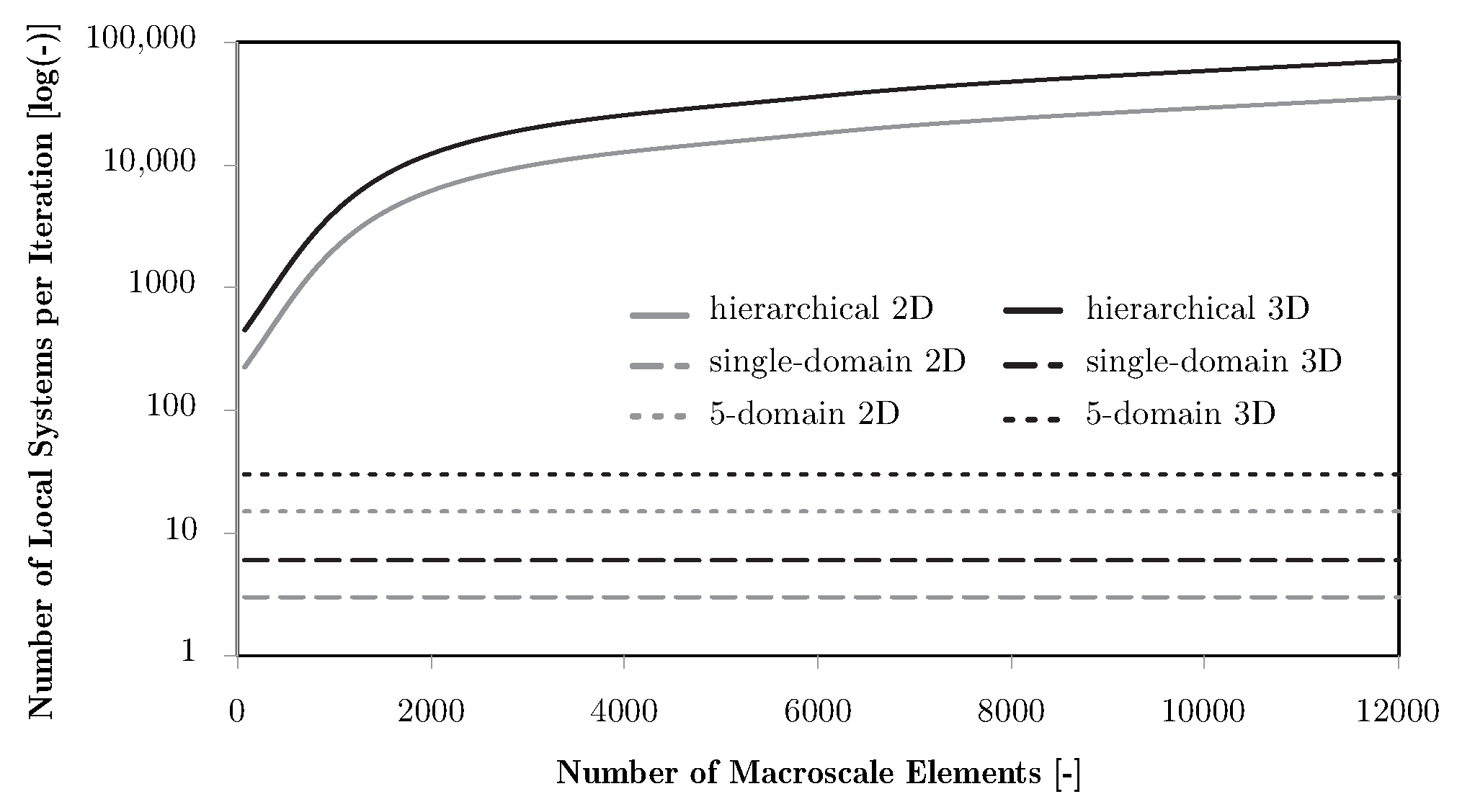
The finite element discretisations for the macro- and microscales differ in both geometry and element type. There is a mesh for the global structure, with its own boundary conditions, and another mesh for the local problems. All local problems use the same mesh definition and apply multi-degree-of-freedom constraints to enforce periodicity of the deformed state required to solve the AEH problems. It is important to note that, in hierarchical formulations, each finite element at the macroscale is associated with its own local problem. For each iteration, besides solving the macroscale problem, this requires solving six finite element equation systems per microscale to obtain the homogenised elastic tensor for 3D problems and three for 2D. Consequently, the total cost grows proportionally to the number of macroscale elements, leading to prohibitive requirements even for moderately refined meshes, even before considering the impact of the increasing number of variables and problems on the optimisation convergence. In contrast, the subdomain approach reduces the number of local problems to the number of predefined subdomains, which is typically several orders of magnitude smaller than the number of elements. The number of systems to be solved per iteration is therefore proportional to the subdomain count, making the computational cost largely independent of mesh refinement. This difference is illustrated schematically in Figure 2, where the scaling with problem size is shown for hierarchical versus subdomain approaches.

4.1. Hierarchical Models

The computational aspects of the general problem of hierarchical topology optimisation are developed by the authors and follow the basic structure shown in several references [8,9,13,25,26,32]. In particular, Coelho [25] divides them between type I and type II strategies. In type I strategies, the problem is solved by acting upon the microscale densities, $\mu$, while the macrostructure densities, $\rho$, are dependent variables. In type II strategies both variable fields are independent and are updated in the respective scale according to the hierarchical definitions (e.g., Equations (8) and (9)). This also allows the use of an additional constraint for the local problems [12].

In the program developed in this work [16], different methodologies are internally classified using H# codes. The first group, H1 to H3, correspond to general hierarchical optimisation approaches. In H1 the optimisation acts only on the microscale densities (type I), while in H3, both macro- and microscale densities evolve simultaneously (type II). The H2 mode represents inverse homogenisation, where only the local problem is solved for a prescribed macroscopic deformation or loading state, and no macrostructural optimisation is performed. The H4 to H6 modes are derived from inverse homogenisation, but adopt different levels of coupling between scales. The H4 and H5 strategies are single-domain modules, where the entire structure is represented by one repeated microscale unit-cell; the difference is that H4 updates only the microscale densities, while H5 updates both scales in a manner equivalent to the general H1 and H3 modes, respectively. The H6 mode is a decoupled approach, where one global macrostructural topology optimisation is performed with a single evolving material distribution, while the microscale problem is solved independently to define an idealised cellular or composite material. Finally, the H7 and H8 modes extend the single-domain idea to multiple subdomains of the macrostructure. Each subdomain has its own microscale problem: in H7, both macro- and microscale densities are updated independently (with the subdomain averages satisfying the global volume constraint), while in H8, the macrostructural density is kept constant and equal to the global constraint, and only the microscale fields evolve. In this sense, H7 is closely related to the general hierarchical H3 mode but with a reduced number of local problems defined by subdomains instead of every finite element. A summary is provided in

Table 1. Summary of optimisation strategies H1–H8 in the in-house code.

Strategy	Description	Application	Performance
H1	Hierarchical: optimisation acts only on microscale densities; macroscale densities are dependent.	Full hierarchical (type I, micro-driven).	High accuracy, very costly.
H2	Inverse homogenisation: the isolated local problem solved for imposed macroscopic fields.	Design of unit-cell materials with target effective properties.	Efficient, but not linked to a global structure.
H3	Hierarchical: simultaneous optimisation of macro- and microscale densities.	Full hierarchical (type II, concurrent macro–micro).	High accuracy, very costly.
H4	Single-domain: optimisation at microscale only, macroscale density fixed to the global volume fraction.	One representative unit-cell optimised for the whole structure.	Very efficient; equivalent to H1 with one local problem.
H5	Single-domain: independent macro- and micro-updates; equivalent to H3 but reduced to one local problem.	Same as H4, used for comparative studies and benchmarking.	Same results as H4 in practice.
H6	Decoupled: macrostructure optimised as a SIMP problem; microscale solved independently.	Structural optimisation with a single global optimal cellular/composite material.	Yields discrete macro- and microstructures.
H7	Subdomain-based: each macro subdomain has its own microscale problem, with both scales updated.	H3-based, regional tailoring of composite structures.	Balances detail and cost; dependent on subdomain definition.
H8	Subdomain-based: constant macro density equal to the global constraint; only microscale updated.	Similar to H7, but a simpler global problem.	More stable and efficient than H7, with slightly less flexibility.

.

While this overview is important to understand the comparison between these strategies, namely in terms of application and computational requirements, the focus of this work is on the more computationally efficient and feasible subdomain approaches. Note that subdomains are usually defined a priori, as a preprocessing task of the macroscale problem, and according to an engineering evaluation of the problem. This program also allows the automatic domain division according to its response and the distribution of a chosen variable (e.g., equivalent or principal stress fields).

4.2. Multiscale Optimisation Algorithms

The two-scale material distribution is reflected in the distribution of a macrostructural density $\rho$ defined for each global structure finite element, $e_{\mathrm{x}}$, and sets of microstructural densities $\mu$ defined for each finite element of each representative unit-cell, $e_{\mathrm{y}}$. The general hierarchical problem involves a mesh of ${\mathrm{N}}_{e_{\mathrm{x}}}$ macroscale finite elements and ${\mathrm{N}}_{e_{\mathrm{x}}}$ meshes of ${\mathrm{N}}_{e_{\mathrm{y}}}$ microscale finite elements. Each macroscale element has an associated local problem, for which the total number of optimisation variables is ${\mathrm{N}}_{e_{\mathrm{x}}}\times {\mathrm{N}}_{e_{\mathrm{y}}}$. For each macroscale element and the respective local problem, the global density and the local densities are related by the local volume constraint defined in expression (10).

The direct application of the optimality criteria defined before leads to the use of the definition of the multiplier (vd. stationarity condition of Equation (29)) [32]:

$$\begin{array}{c}\hfill {\gamma }^{e_{\mathrm{y}}}={\displaystyle \frac{\mathrm{\Pi }}{{\mathrm{\Lambda }}_t}}.\end{array}$$

(31)

$\mathrm{\Pi }$ defines the local sensitivity to the variation in $\mu$ in element $e_{\mathrm{y}}$ of the microscale of element $e_{\mathrm{x}}$ and can be defined, for the elasticity hierarchical problem, as

$$\begin{array}{c}\hfill \mathrm{\Pi }=\left[{\displaystyle \frac{\partial D_{ijkl}^{\mathrm{h}}\left(\mu \right)}{\partial \mu \left(y\right)}}{\langle {\epsilon }_{ij}\left(\tilde{\mathbf{u}}\right)\rangle }_{e_{\mathrm{x}}}{\langle {\epsilon }_{kl}\left(\tilde{\mathbf{u}}\right)\rangle }_{e_{\mathrm{x}}}\right].\end{array}$$

(32)

${\langle {\epsilon }_{ij}\left(\tilde{\mathbf{u}}\right)\rangle }_{e_{\mathrm{x}}}$ is the macrostructural strain for element $e_{\mathrm{x}}$, localised to allow the processing of the local problem. This is an average value for this element. The same can be performed for the subdomain problem, where $\mathrm{\Pi }$ becomes

$$\begin{array}{ccc}& & \mathrm{\Pi }=\hfill \\ & & {\displaystyle \frac{\partial {\langle D_{ijkl}^{\mathrm{h}}\left(\mu \right)\rangle }_{{\mathrm{\Omega }}_q}}{\partial \mu \left(y\right)}}\sum _{e=1}^{\mathrm{N}}{\displaystyle \frac{V_{e_{\mathrm{x}}}}{V_{\mathrm{\Omega }}}}\left[\phantom{{\displaystyle \frac{\mathrm{x}}{\mathrm{x}}}}{\langle {\epsilon }_{ij}\left(\tilde{\mathbf{u}}\right)\rangle }_{e_{\mathrm{x}}}{\langle {\epsilon }_{kl}\left(\tilde{\mathbf{u}}\right)\rangle }_{e_{\mathrm{x}}}\right].\hfill \end{array}$$

(33)

$\langle D_{ijkl}^{\mathrm{h}}\left(\mu \right)\rangle$ is the homogenised constitutive matrix for the subdomain ${\mathrm{\Omega }}_q$. The brackets $\langle ·\rangle$ are used to indicate the fact that this material is a response to an average along a given domain. $N=N_{e_{\mathrm{x}}\in {\mathrm{\Omega }}_q}$ is the number of macroscale finite elements in the subdomain, and ${\langle {\epsilon }_{ij}\left(\tilde{\mathbf{u}}\right)\rangle }_{e_{\mathrm{x}}}$ is the average of the global strains for the elements $e_{\mathrm{x}}$ of ${\mathrm{\Omega }}_q$. ${\mathrm{\Omega }}_q$ is each the Q subdomains in the strategies H7 and H8. In the strategies H4 and H5, ${\mathrm{\Omega }}_1$ is the whole problem domain $\mathrm{\Omega }$ ($Q=1$).

Since, in this case, the localisation process uses the macroscale strains as an average from a given domain, some relevant aspects of the overall behaviour can become diluted. This may lead to an optimal solution that is ideal for an average field but not for the effective structure’s needs. This problem can be numerically controlled using an alternative average to the volume evaluation of the domain. The use of a modified problem, weighting different aspects of the mechanical behaviour of the structure, may allow this limitation to be surpassed. This leads to a sensitivity evaluation, using the weighting parameter $\iota$, which can be defined as

$$\begin{array}{ccc}& & \mathrm{\Pi }=\hfill \\ & & {\displaystyle \frac{\partial {\langle D_{ijkl}^{\mathrm{h}}\left(\mu \right)\rangle }_{{\mathrm{\Omega }}_q}}{\partial \mu \left(y\right)}}\sum _{e=1}^{\mathrm{N}}\iota {\displaystyle \frac{V_{e_{\mathrm{x}}}}{V_{\mathrm{\Omega }}}}\left[\phantom{{\displaystyle \frac{\mathrm{x}}{\mathrm{x}}}}{\langle {\epsilon }_{ij}\left(\tilde{\mathbf{u}}\right)\rangle }_{e_{\mathrm{x}}}{\langle {\epsilon }_{kl}\left(\tilde{\mathbf{u}}\right)\rangle }_{e_{\mathrm{x}}}\right].\hfill \end{array}$$

(34)

$\iota =1$ leads to the volume average seen before.

A parameter ${\gamma }^{e_{\mathrm{y}}}$ is used to control the updating scheme for optimality criteria methods at each microscale element $e_{\mathrm{y}}$. With it, the microscale density field can be updated for the iteration $t+1$, with [9,32]

$$\begin{array}{c}\hfill {\mu }_{t+1}^{e_{\mathrm{y}}}=\left\{\begin{array}{c}max\left[(1-\zeta ){\mu }_t^{e_{\mathrm{y}}},{\mu }_{min}\right]\hfill \\ \mathrm{if}{\gamma }^{e_{\mathrm{y}}}{\mu }_t^{e_{\mathrm{y}}}\le max\left[(1-\zeta ){\mu }_t^{e_{\mathrm{y}}},{\mu }_{min}\right]\hfill \\ \\ min\left[(1+\zeta ){\mu }_t^{e_{\mathrm{y}}},1\right]\hfill \\ \mathrm{if}{\gamma }^{e_{\mathrm{y}}}{\mu }_t^{e_{\mathrm{y}}}\ge min\left[(1+\zeta ){\mu }_t^{e_{\mathrm{y}}},1\right]\hfill \\ \\ {\gamma }^{e_{\mathrm{y}}}{\mu }_t^{e_{\mathrm{y}}}\hfill \\ \mathrm{if}\mathrm{otherwise}\hfill \end{array}\right..\end{array}$$

(35)

The move limit $\zeta$ controls the update change for each variable. At the optimum, ${\gamma }^{e_{\mathrm{y}}}=1$ for all the densities. This material distribution allows the calculation of a new macroscale density value, for the respective element $e_{\mathrm{x}}$, as

$$\begin{array}{c}\hfill {\rho }_{t+1}^{e_{\mathrm{x}}}={\int }_{Y_{e_{\mathrm{x}}}}{\mu }_{t+1}\mathrm{d}Y,\end{array}$$

(36)

and the calculation of new homogenised constitutive matrices. These are used at the macroscale to provide constitutive information to solve the equilibrium problem, where the strain fields are calculated and used at the following iteration to once again evaluate and update the microscale densities. The macroscale densities are used to update the global volume constraint Lagrange multiplier as

$$\begin{array}{c}\hfill {\mathrm{\Lambda }}_{t+1}=max\left[0,{\mathrm{\Lambda }}_t+c\left({\int }_{\mathrm{\Omega }}{\rho }_t\mathrm{d}\mathrm{\Omega }-\overline{V}\right)\right].\end{array}$$

(37)

Note that this is a methodology centred on the control of the local densities, with the global densities acting as dependent variables. This is explicitly taken from the optimal criteria defined before [8]. It has some limitations, namely in terms of the calibration difficulties of the augmented Lagrangian approach [25]. In addition to this approach, several different strategies are used with the integration of Krister Svanberg’s Method of Moving Asymptotes (MMA) [18]. Following type I and type II configurations [33], this method allows the processing of a large number of optimisation variables with great efficiency and flexibility. Moreover, with little changes, it can be made to behave as the CONvex LINearisation method (CONLIN) [19,20]. All of this can be performed by acting over all the microscale densities simultaneously in a type II configuration, updating both scale density fields, and keeping the local problems totally separate. In this case, the updated macroscale variables act as local volume constraints as $V_Y\left(\mu \right)={\rho }_{e_{\mathrm{x}}}{\overline{V}}_Y$. The Lagrange multipliers of the local problems are used as sensitivities to update the respective macroscale densities [25]. There are several different algorithm combinations, but the results shown in this work use MMA for the macroscale update, and either MMA or CONLIN for the microscale update. The local Lagrange multipliers are essential to the stability of the whole process. In this aspect, CONLIN tends to provide better multipliers than MMA in the local problem, allowing for a more stable convergence control [12,16]. Even so, this work keeps MMA as the main algorithm in both scales, since the subdomain problem tends to be more stable because of the smaller number of local problems. CONLIN is nevertheless used for comparison in some examples presented in this work. Moreover, the H8 strategy differs from H7 because it only updates the local variables. In this sense, the H8 method imposes the same volume constraint and is equal to the global volume constraint at each of the local problems, keeping the macrostructural densities locked accordingly.

Another aspect that is relevant in this work is the use of sensitivity filtering techniques [9]. This is usually used to control instabilities, like checkerboard patterns in penalised topology optimisation problems. In this type of multiscale problem, it also helps to keep a certain level of intermediate microscale densities in the transitions between material and a void, so that the local Lagrange multipliers are kept valid for the stability conditions. However, they also tend to simplify the local topologies, which can lead to some anisotropies of the material.

5. Multiscale Optimisation Results

Based on the “MBB” [9,34] beam bending problem, different boundary conditions, multiscale definitions and mesh configurations are solved over the next sections. In addition to the bending problem, boundary conditions for shear and tension cases are also studied, as shown in Figure 3. Moreover, to further test the coherence of the results, a compression case (without instabilities) is studied by inversion of the tension case. Except when explicitly defined otherwise, the local meshes use $40\times 40$ linear quadrilateral elements. Unlike the hierarchical approach, the subdomain multiscale definition does not significantly increase its computational weight with the size of the macrostructural mesh. As a reference example consider Figure 4, where a full hierarchical bending problem is solved, with a microscale problem for each finite element of the macroscale mesh. This results in a number of local problems proportional to the macroscale refinement level, rendering the computational weight prohibitive, and the balance between structure detail, feasibility (for both each microstructure and algorithm transitions), and processing requirements very hard to balance. In this case, since the subdomain approach requires a number of local problems dependent on the number of domains and not the quality of the macroscale, different macroscale mesh refinements are compared, using $15\times 5$ (M1), $30\times 10$ (M2), $60\times 20$ (M3), $120\times 40$ (M4), and $240\times 80$ (M5) linear quadrilateral finite elements. The global volume constraint uses a volume fraction $f_{\mathrm{v}}=0.5$ of the domain volume $V_{\mathrm{\Omega }}$. The conventional SIMP approach ($d_{\mathrm{m}}=0.0$) is used in most cases. The problems are also solved using a sensitivity filtering technique. In addition to the stability implications, since this work is oriented for applications to composite materials, the way that the filtering tends to keep the topologies simple by smoothing out some details is welcome here.

5.1. Single Domain Approach

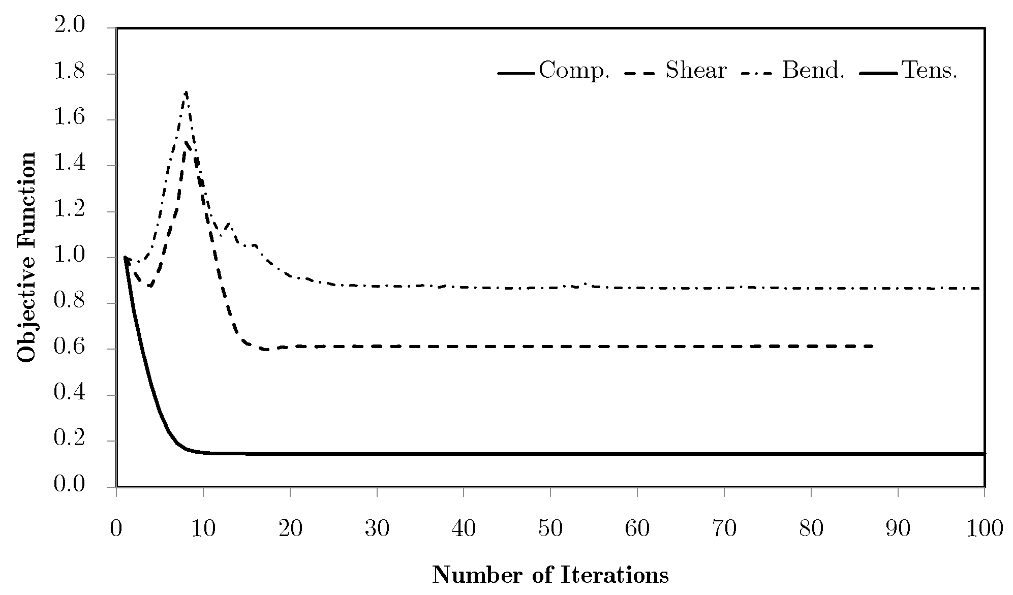
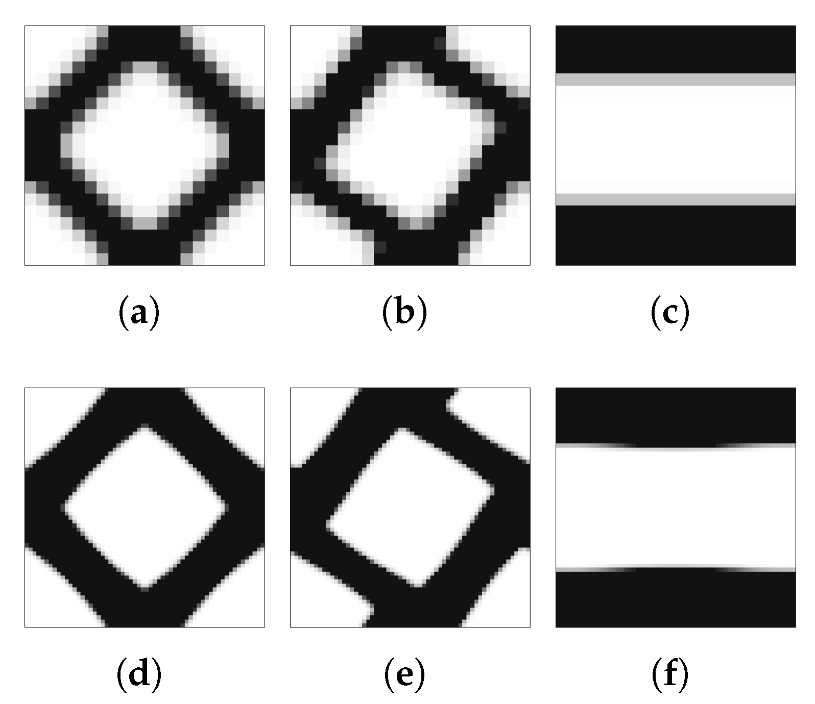
The chosen problems are used to compare the performance of the methods against known behaviour patterns. The first strategies tested are H4 and H5, for which there is only one microscale repeated over all of the problem domain. According to the structural optimisation problem defined earlier, Figure 5 shows the normalised objective function evolution for these problems, using mesh M5. This is the worst case, as will be discussed. First of all, both strategies provide exactly the same results. Initially, these strategies were tested using a structure equivalent to the corresponding hierarchical cases, with one microscale per macroscale finite element. In this sense, H4 used only microstructural density variables, optimised at each iteration as part of a big problem, while the H5 strategy used both macro- and microstructural densities as independent variables, with separated local problems. The only difference to the hierarchical approach was that the sensitivities were calculated as defined in Equation (33), which should result in an equal behaviour for each local problem and a constant microstructure and macroscale density for all of the domain. Since the problem behaviour was expected, the structure of these problems was then changed to take full advantage of the single domain definition. This made sense only if just one local problem was solved for all of the domain, making the problem much smaller than the original hierarchical structure. Moreover, it could provide an optimal material configuration tailored to a given structure. In a way, it is similar to an inverse homogenisation approach, but allows the direct influence of the material on the structure and provides results that are closer to the real problem. The local optimal topologies for each case are shown in Figure 6. These make sense at first glance, but will be further discussed ahead.

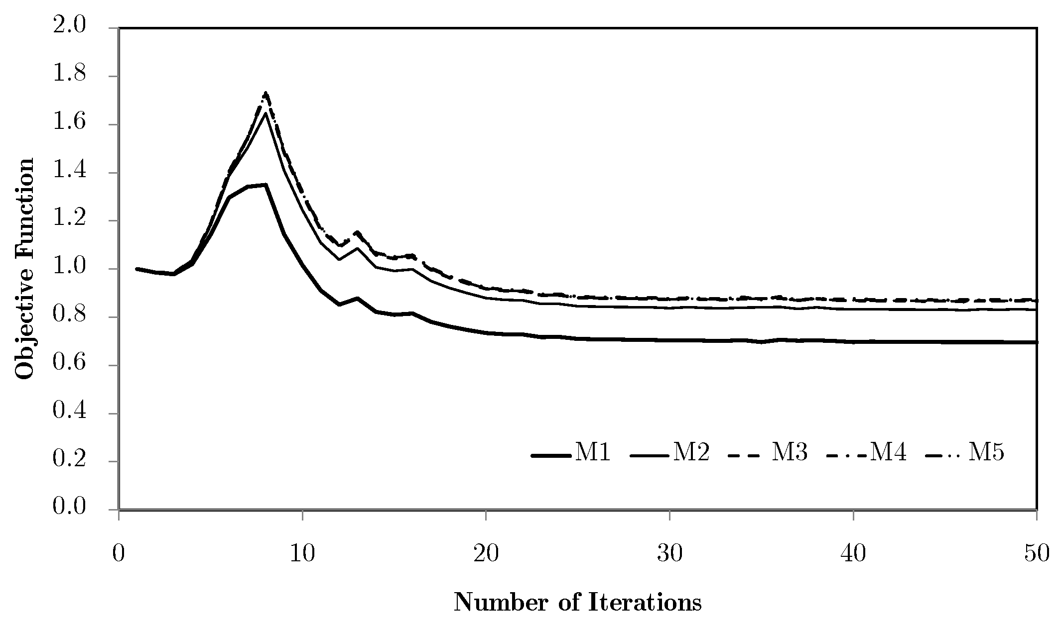
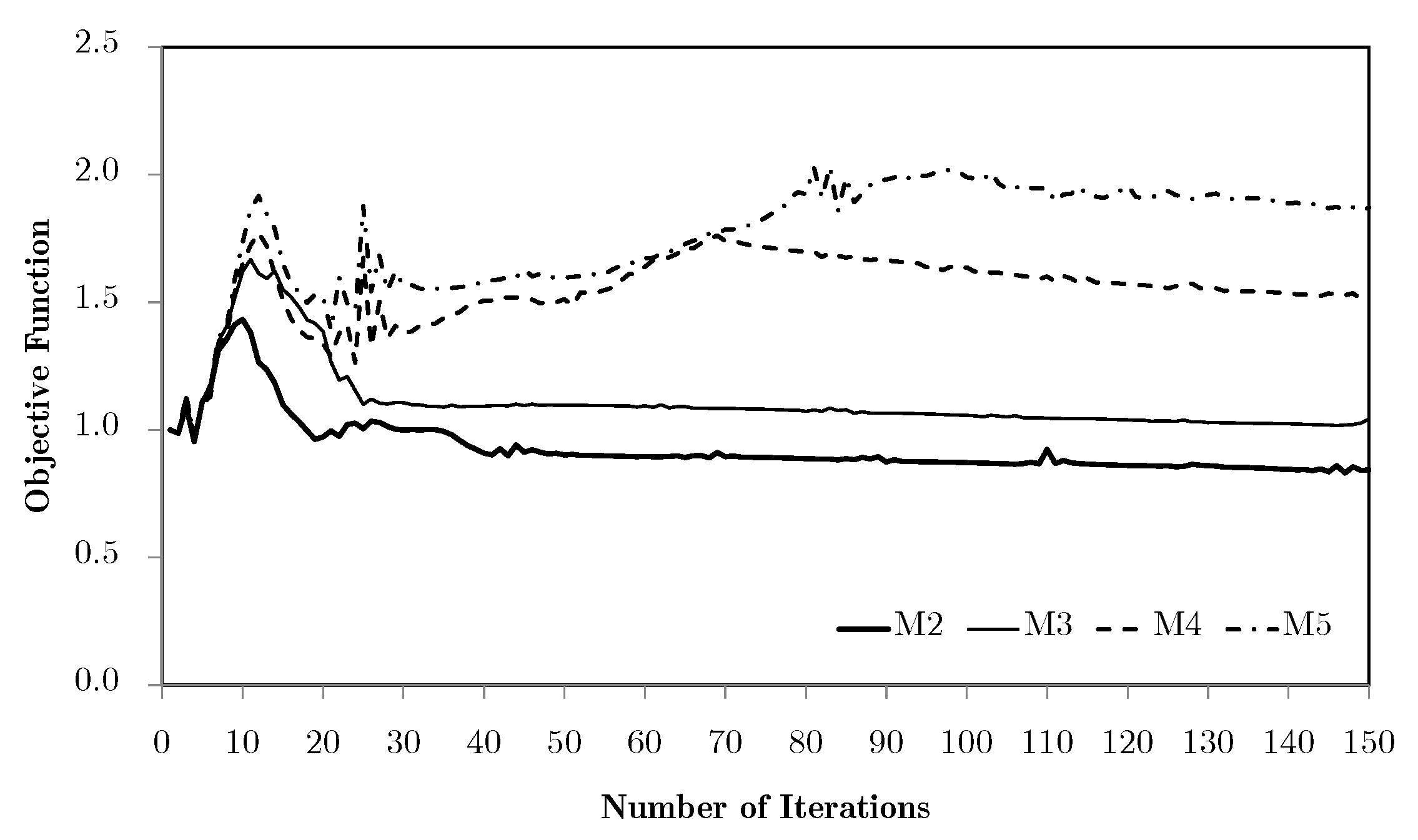
Using different macroscale mesh refinements, the evolution curves are basically coincident for the tension/compression cases. However, for the shear and especially the bending problems, mesh refinements appear to have a negative influence. This issue is essentially rooted in the macroscale mesh. Figure 7 compares the bending problem results for meshes M1 to M5.

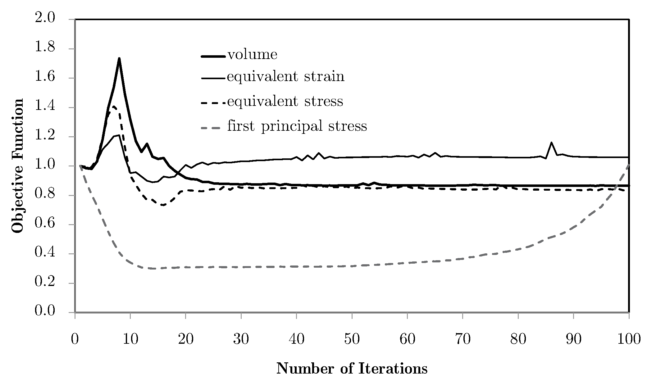
The shown dispersion, with the refinements leading to worse results, comes from the volume weighing of the localised information of all of the domain (vd. Equation (34)). The use of different weights leads to different results, as shown in Figure 8. A numerical parameter is used to activate the different $\iota$ weight options, namely the basic volume average of macroscale strains, as used in the base problem, or using other physical magnitudes as correcting weights, such as equivalent strains, equivalent stresses, or the first principal stresses.

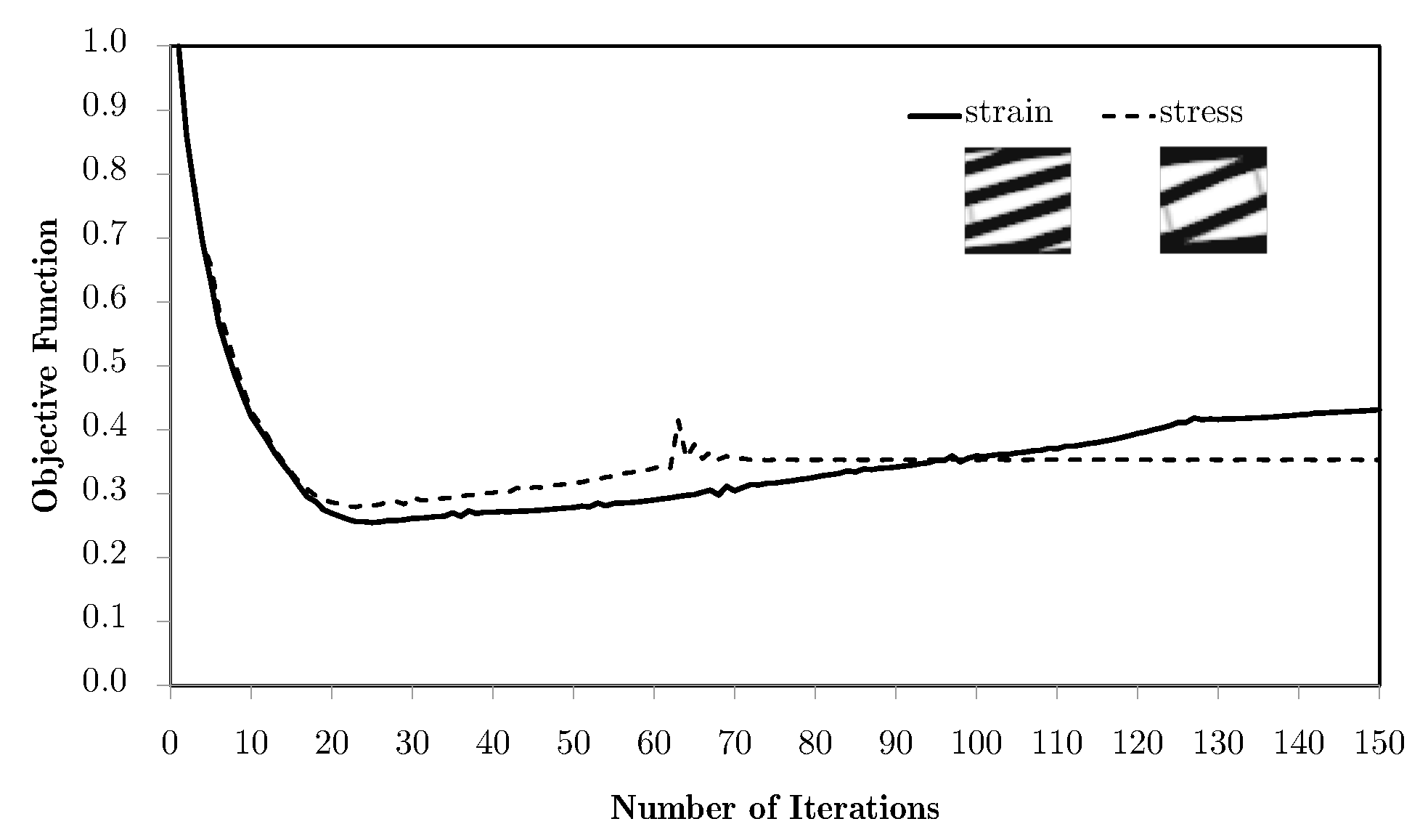
Pondering equivalent stresses leads to slightly better results, as the use of equivalent strains destabilises the process and gives a worse response. In spite of being apparently similar, the stress and strain fields are, in this case, topologically different. This is due to the fact that the stress field is essentially the strain field operated by constitutive tensors. Since the material is anisotropic, this leads to a distortion of the field, leading to different influences. In all these cases, the main limitation of this method for bending problems is the way in which the average tends to cancel the influence of the more relevant structure areas. The response should be dominated by the material orientation dictated by the areas away from the neutral axis, for which the strain and stress levels are higher and where a horizontal material orientation would be ideal. Instead, since these are opposite in signal, the average over the domain tends to be zero. This is why the local topologies obtained for the bending case are so close to the shear ones. Note that this is not a pure bending problem. Even so, these show topologies close to the ones shown in the bibliography [31]. This phenomenon tends to worsen for refined macroscale meshes because of the increasing number of different contributions, which approximates the average of zero for the axial components of strain. Nonetheless, other weighting options can solve this problem. One of them is using the principal stress ${\sigma }_1$. In this case, weighting privilege is given to areas that are tension-oriented in terms of loading, making this average more compatible with this problem. The problem stabilises fairly quickly and with a very good response. However, the process here is allowed to continue in order to show a subsequent effect. With the evolution of the iterative process, the use of filtering of sensitivities tends to slowly keep updating the solution. Note that the use of filters over the sensitivities, using the influence of neighbour elements, numerically deviates the problem from its original response to a smoothed response, making the sensitivity evaluation more according to the non-local elasticity theory. In this case, it leads to a gradual and slow orientation of material along a preferred direction, gradually becoming a laminate. This is a desired effect with two-material distributions, but becomes a problem with a material/void distribution. As the material tends to become laminar, the void phase gradually becomes continuous, leading to a lack of connection (and stiffness) between the material phases. Note that this effect does not pose a problem with two-material configurations. Moreover, this effect does not even occur without the use of filtering strategies.

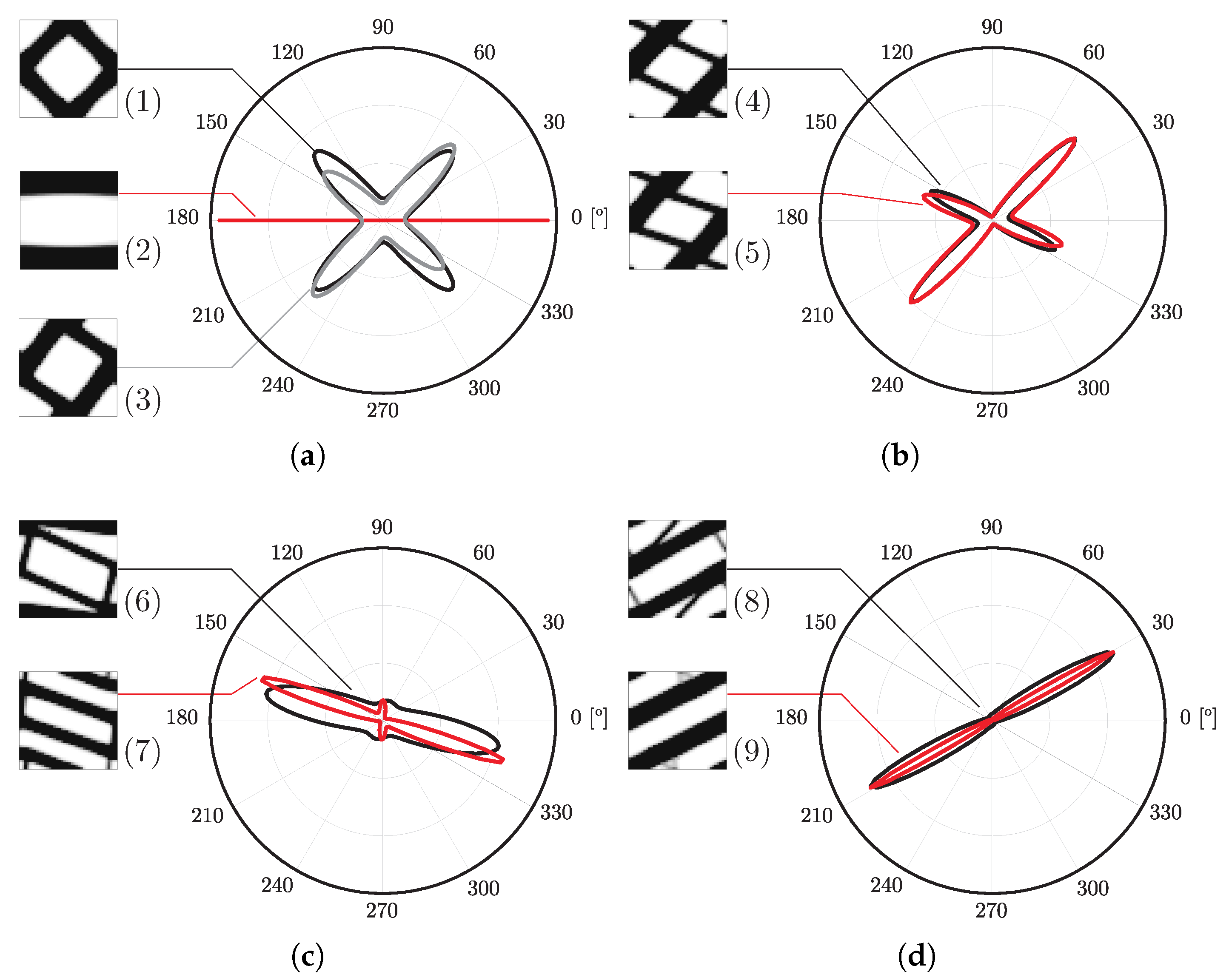
Figure 9 provides further detail, as the local topologies for each case are shown with the respective anisotropy plot for stiffness orientation. The anisotropic response is coherent with the loading. This fact is evident in tension/compression cases. For the bending cases, the orientations are not ideal because of the problems discussed before. Stiffness is too orientated towards the shear response. The material presents a high stiffness in diagonal directions, but is too flexible in the horizontal alignment needed for the response. This can even be lower than the initial guess. The use of different weighting variables can effectively make the response much better. Note the case using the principal stress ${\sigma }_1$. The laminate’s lack of transversal stiffness is also illustrated. The use of a principal stress ${\sigma }_2$, for example, results in worse performance.

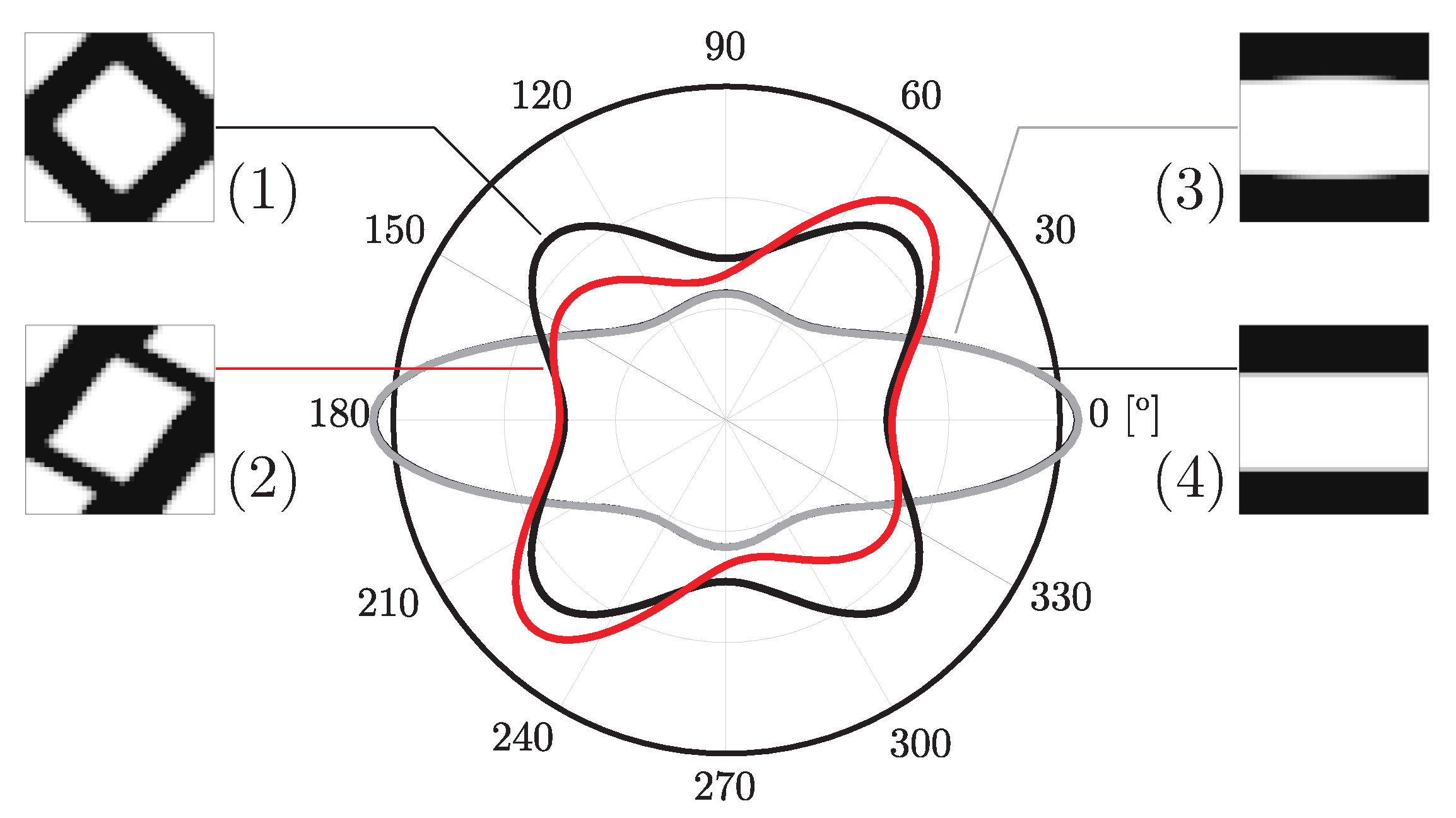
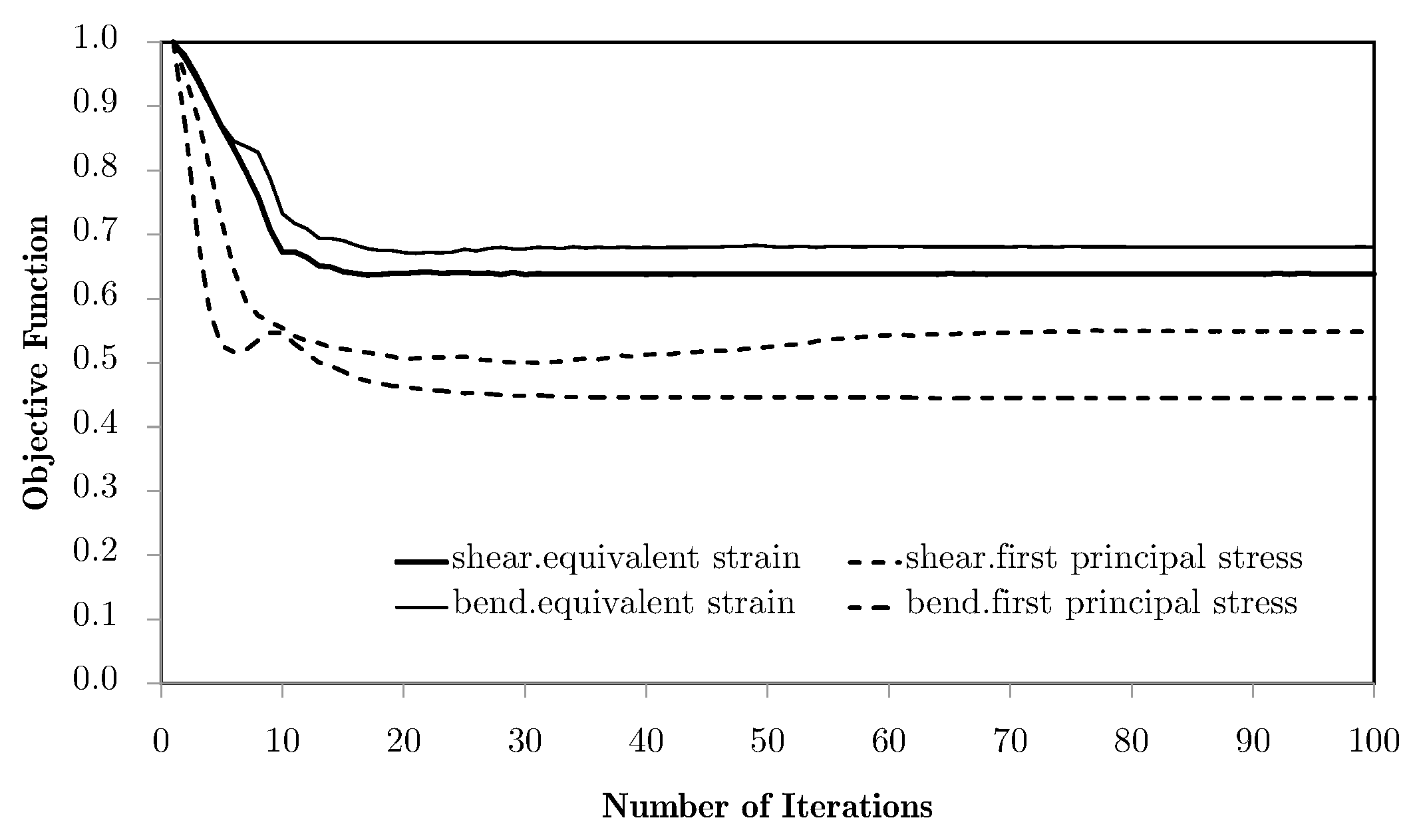
Using closer phase properties, with $d_{\mathrm{m}}=0.1$, the results are much better, as expected. This is due not only to the higher stiffness of the soft phase when compared to the void used before, but also to the fact that the laminate’s lack of physical connection between phases is no longer a problem. In addition, the topologies tend to be even simpler, making the filtering effect useful from a composite material perspective. The lamination tendency arises because sensitivity filtering smooths the transition between material and a void, gradually favouring layered patterns. While this can be beneficial in two-material optimisation, it reduces connectivity in material/void problems. Practically, this effect can be mitigated by (i) adopting alternative weighting schemes (e.g., principal stresses), (ii) selecting subdomain divisions aligned with stress paths, or (iii) constraining the minimum feature size to prevent extended laminates. These guidelines help practitioners avoid non-physical solutions without requiring additional computation. Figure 10 shows local topologies and anisotropy plots for the least favourable case over the previous examples (equivalent strain weighting), showing that even in that case, the results are much better. This is also shown with the objective function evolution (vd. Figure 11), where there is much more evident energy minimisation. In the case of principal stress weighing, ${\sigma }_1$, the minimisation is performed for levels comparable to the ones shown before, but, above all, is significantly more stable.

Figure 12 shows topologies for different refinement levels of the microscale mesh, using $20\times 20$ and $60\times 60$ finite elements. The results show the same basic shapes, and in this implementation, the local refinement tends to influence, to a much smaller degree, the overall quality of the results than the macrostructural meshes. Even so, the lack of detail of coarse meshes tends to result in more flexible results. This can become a relevant problem in cases where, even for filtered problems, there is the need for a certain degree of topological detail.

5.2. Subdomain Multiscale Optimisation

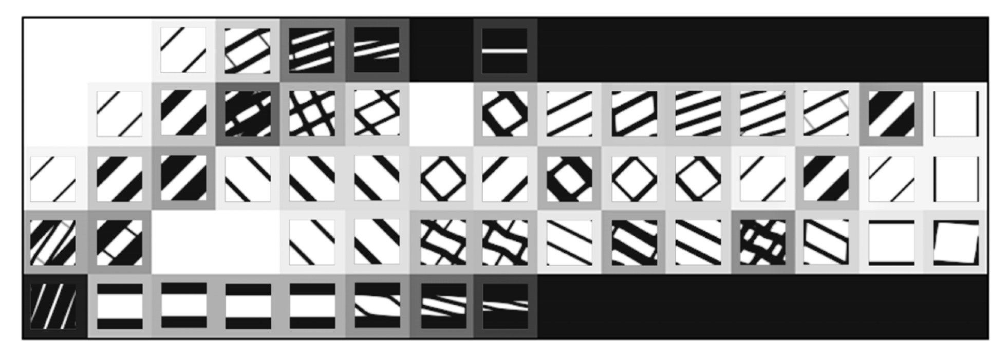
The optimisation modes H7 and H8 represent an alternative in multiscale topology optimisation, controlling the number of local problems in a hierarchical approach. In these cases, the procedures are derived from the H5 case seen earlier, adopting a methodology that considers the macro- and microscale density variables as independent, but with a strain localisation weighting performed by subdivisions of the local domain. There is a local problem for each macrostructure subdomain. The main aim of this strategy is to balance the search for optimal material distribution and the fabrication of structural components from composite materials. The difference between the H7 and H8 modes is in the macroscale density variable. In the H8 strategy, this is fixed and equal to the global volume fraction, making each of the local problems constrained by the same volume fraction. Figure 13 shows some examples of subdomain divisions for the geometry used in the previous tests.

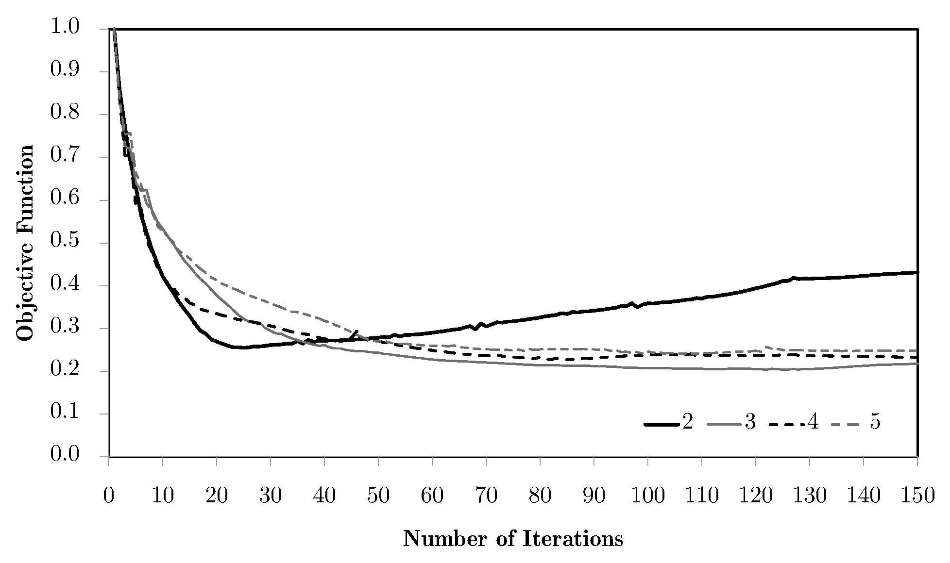
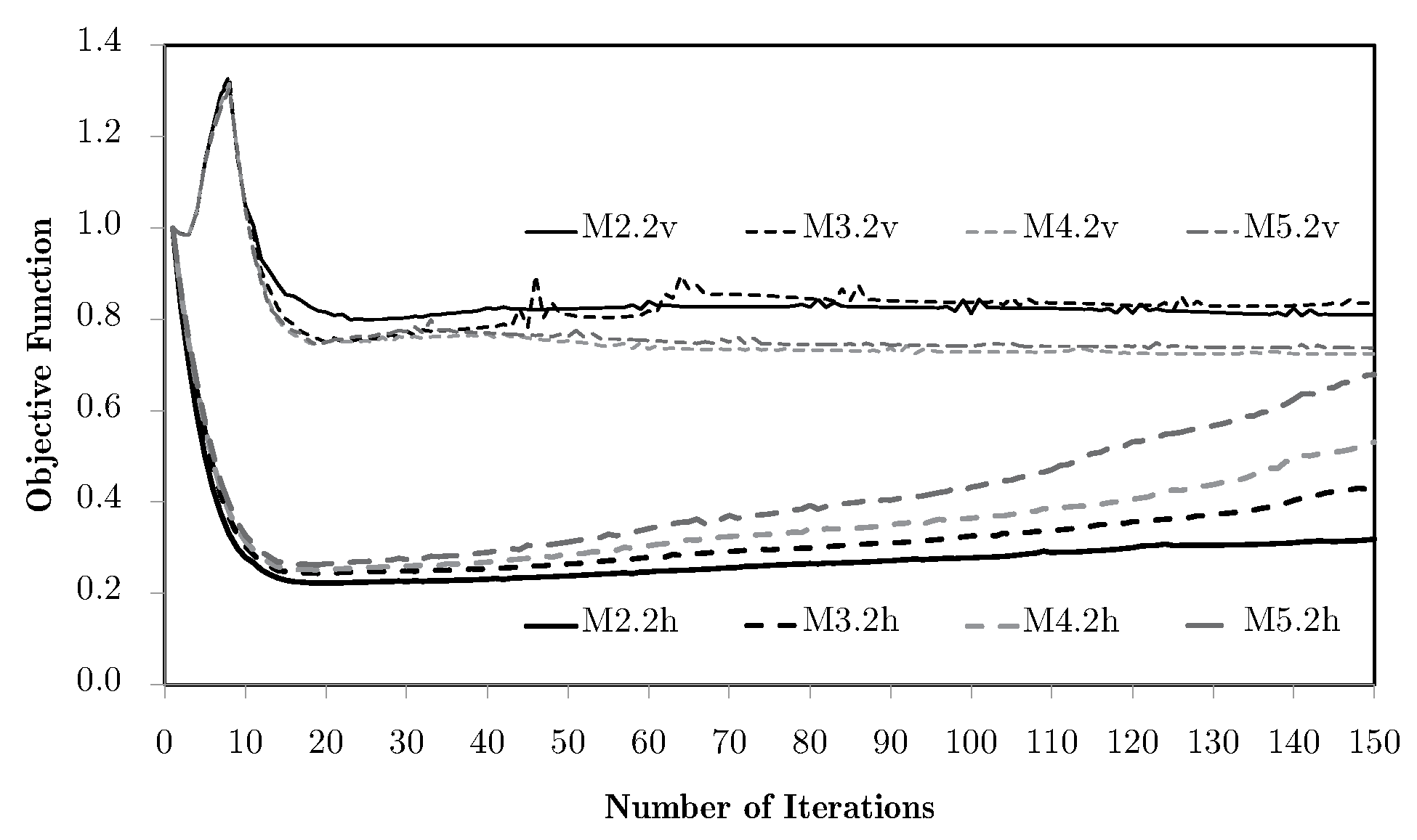
Going back to the previous problem of bending with equivalent strain weighting, as the one with the worst results, Figure 14 shows the objective function evolution for two horizontal subdomains and different levels of macroscale mesh refinement, using the H7 method. In this case, with only two local problems and two RUC, the results are immediately much better.

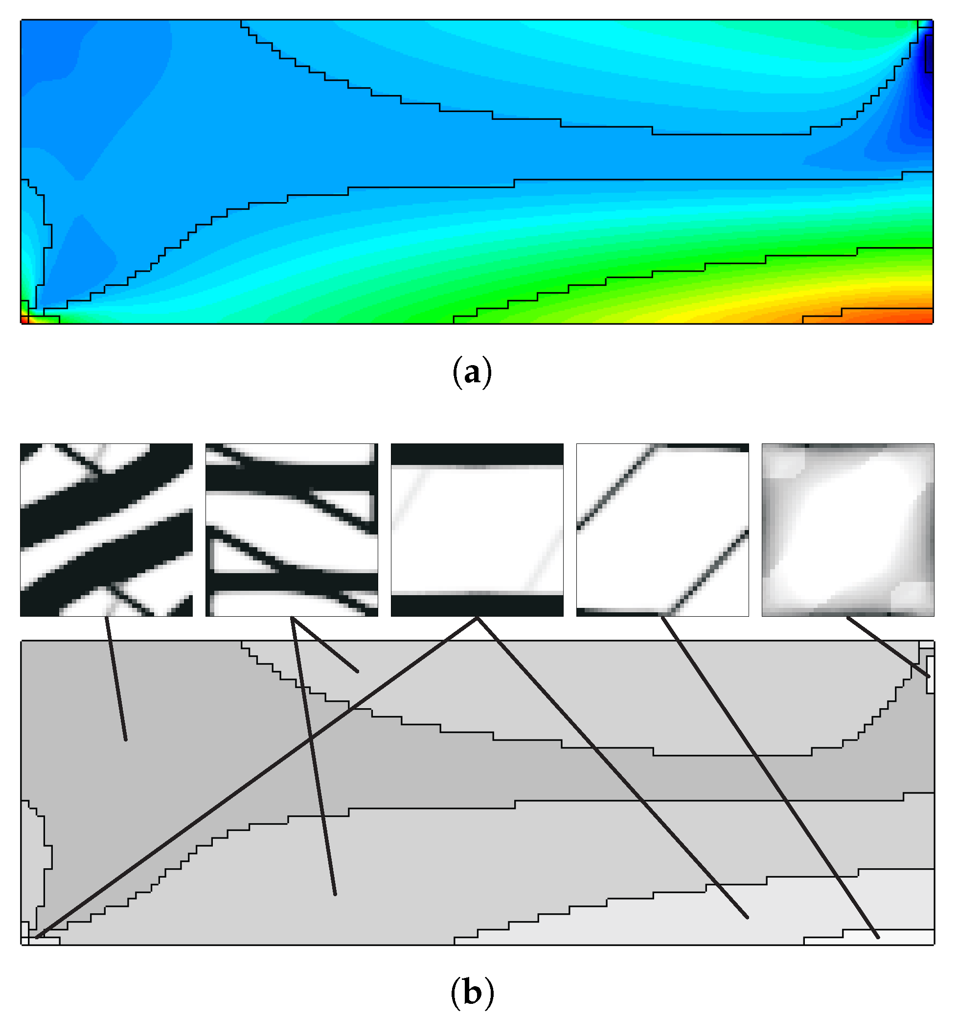
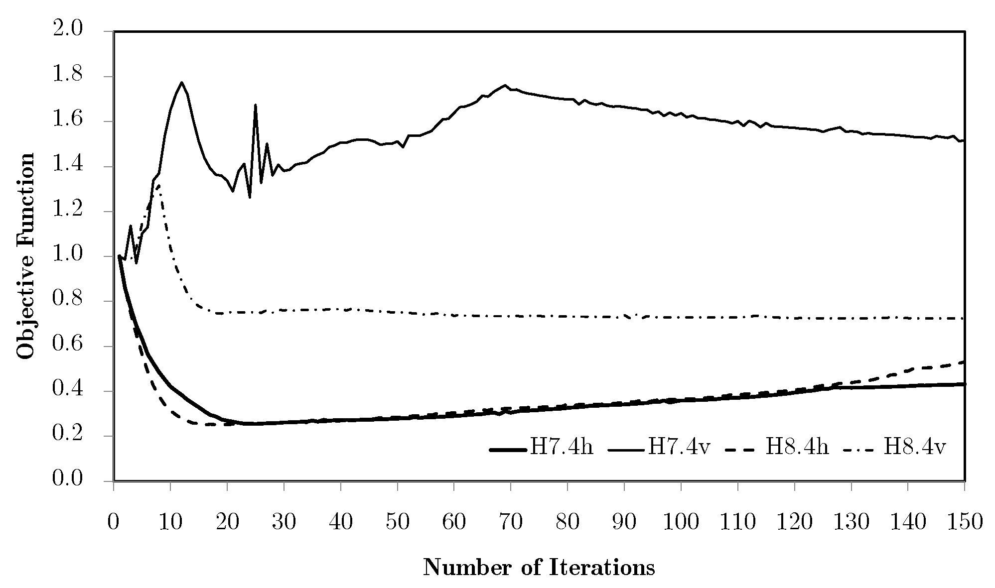
However, the same analysis for vertical subdomains (vd. Figure 15) leads to apparently contradictory conclusions. This is due to the inadequacy of vertical domains to the bending problem, just as the one-domain problem seen before. While the horizontal divisions tend to be less prone to the problems seen before, the vertical divisions make the geometry closer to a set of thicker beams, which makes the problems worse. This shows that the subdomain approach needs a coherent engineering evaluation of the divisions according to the specific problem, so that it makes sense for the service requirements of the structure. The difference between horizontal and vertical divisions in bending cases stems from the stress and strain distribution. Bending produces tensile and compressive regions separated by a neutral axis. Subdomains aligned with this axis (horizontal divisions) capture the contrasting behaviours effectively, while vertical divisions tend to average them out and lead to less meaningful optimisation. From an engineering standpoint, this mirrors the way laminates and composites are often designed with through-thickness variation rather than crosswise partitioning. Note that automatic division schemes are possible, as seen for the example shown in Figure 16. In this case, the division is performed according to the principal stress (e.g., ${\sigma }_1$) field. Note that in this case, solved with the H7 method, macroscale densities are tied to the microscale material distributions, with the representation of the corresponding grey level between 0 and 1.

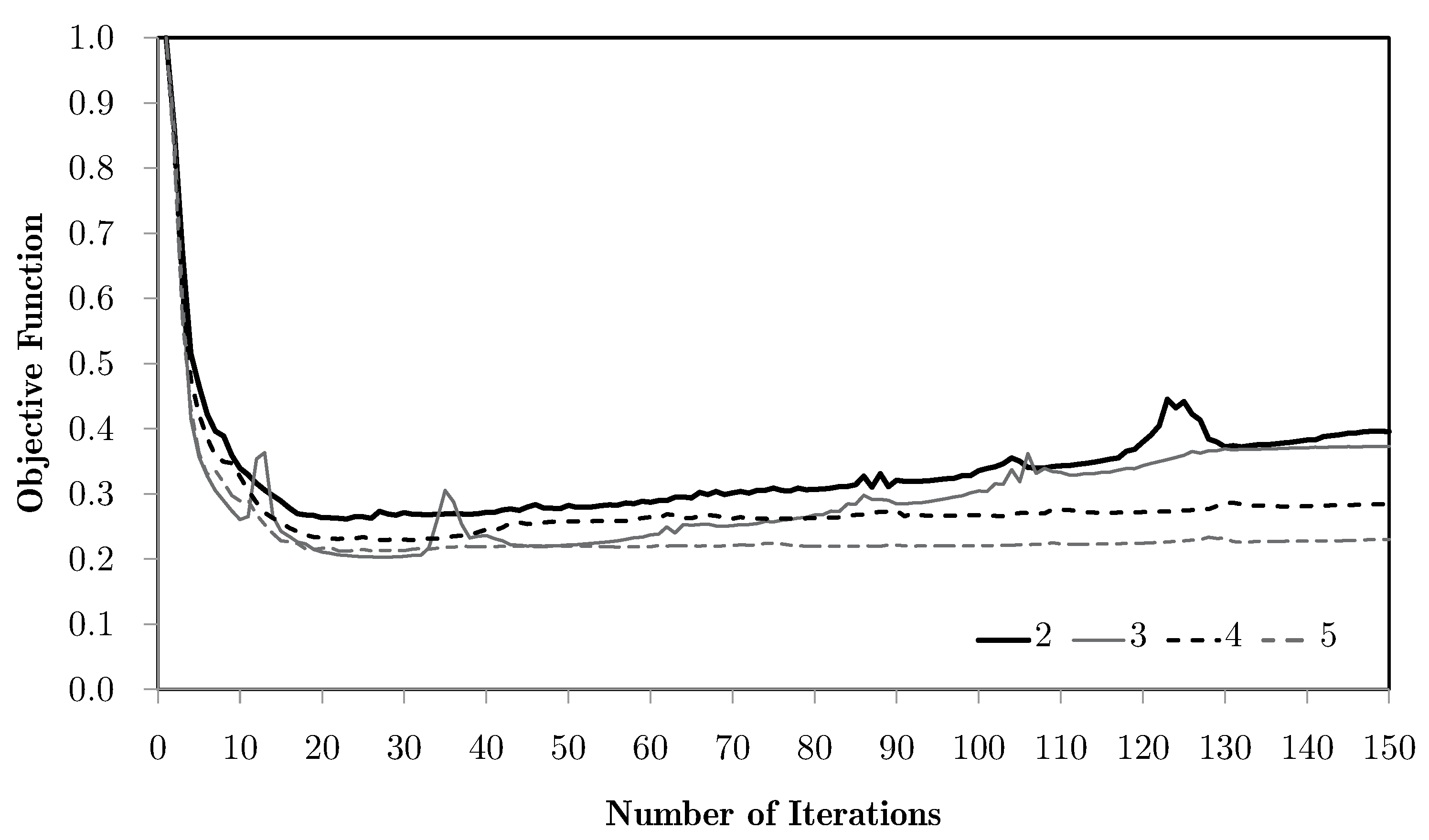
Going back to the predefined divisions, Figure 17 shows the evolution of the objective functions for different combinations of horizontal domains. As an example, mesh M4 is used. The worst results are the ones for two divisions, where, at the same time, increasing the number of divisions makes the average values more representative and the results better. Comparing again with Figure 14, one can observe that the two division case has a gradual deterioration of the results because of the filtering and topology simplification. However, the problem stability is kept, as can be seen in Figure 18, where the Lagrange multipliers $\lambda$ for each of the local problems converge in a stable manner. Once again, this phenomenon is related to the tendency of some local topologies to evolve to simple laminates. Nevertheless, this is a numerical phenomenon that is more controlled with the H7 method using the alternative weighting options, like equivalent stress instead of strains, as shown in Figure 19. In spite of an initial simplification, the topology stabilises before it becomes a real issue, without the lack of material connectivity seen before for material/void problems.

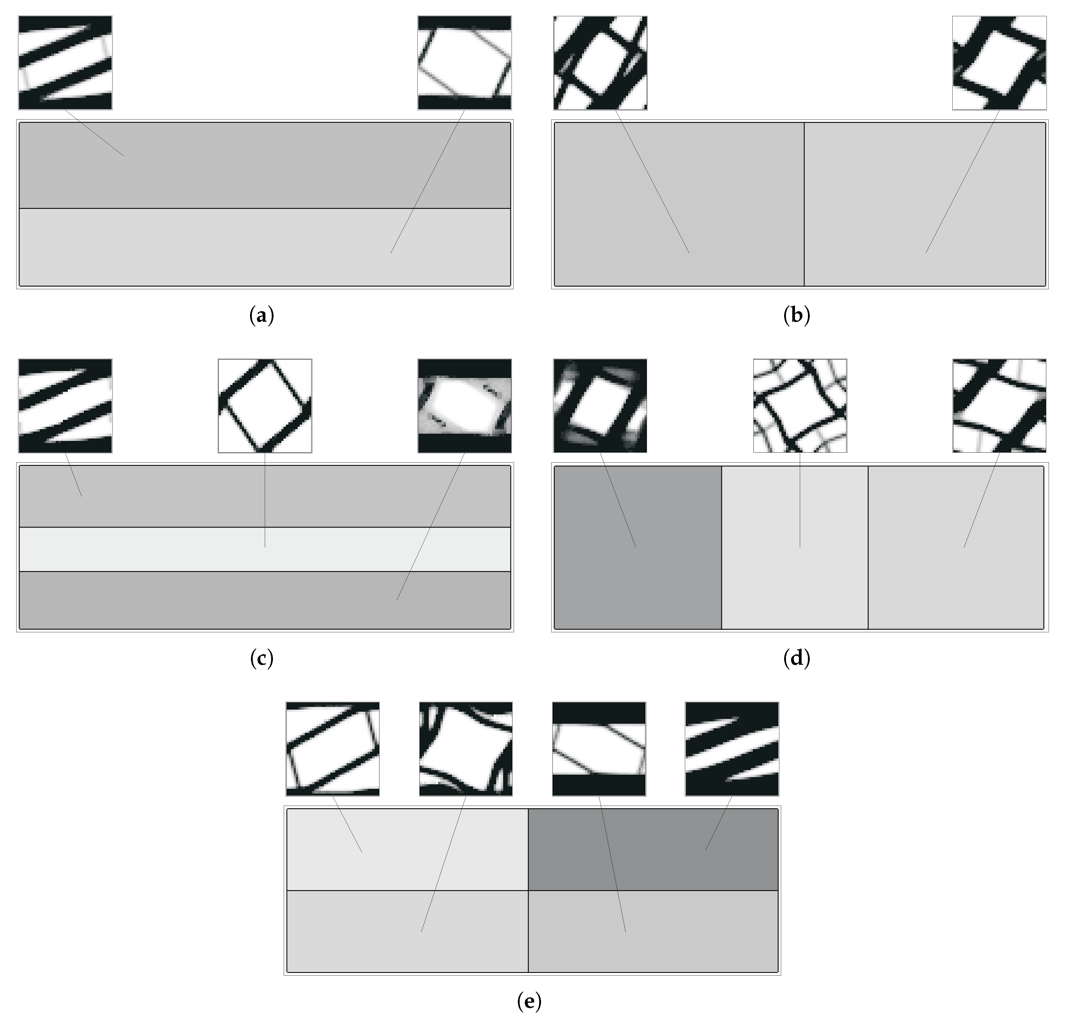
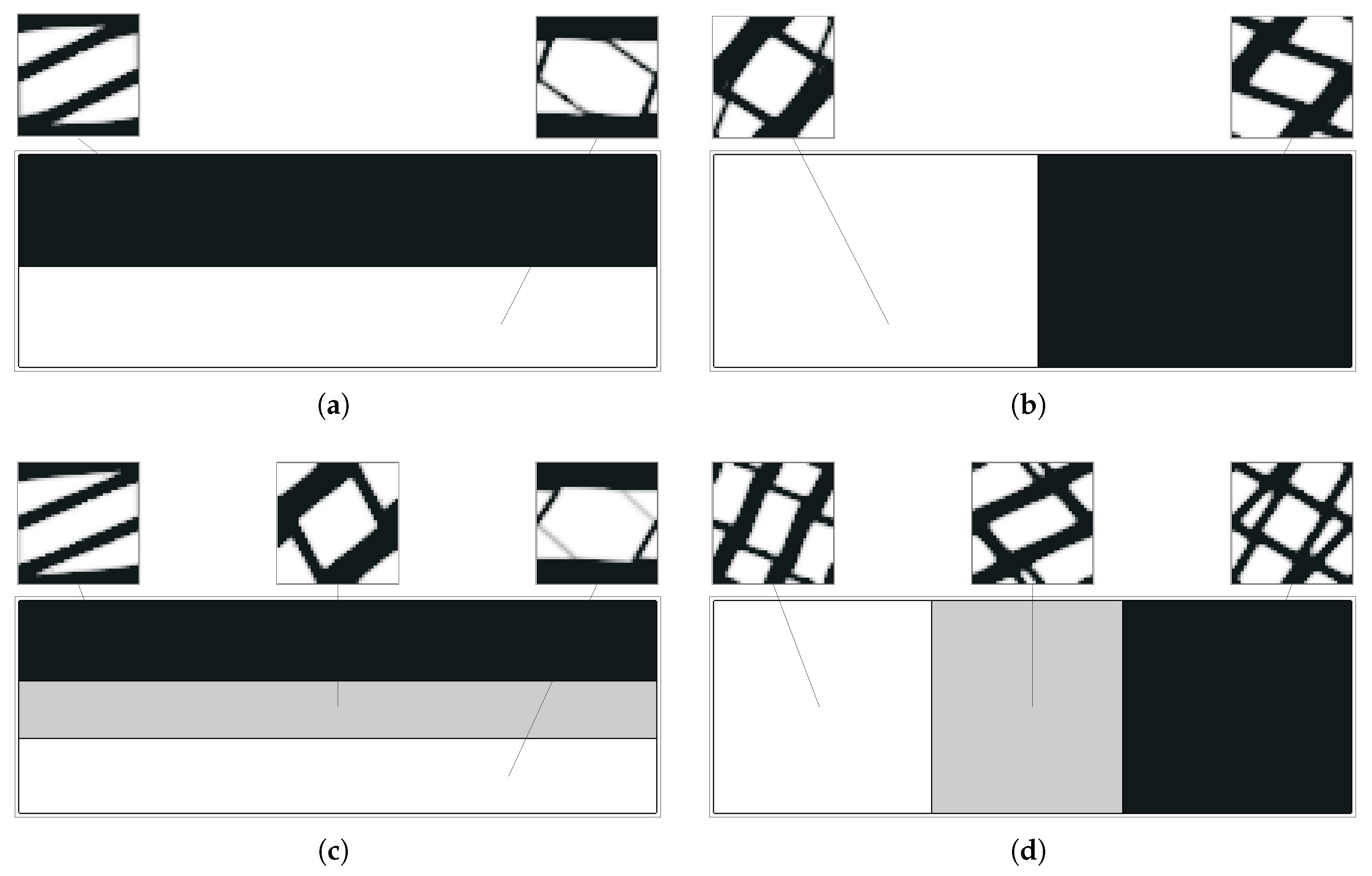
Figure 20 and Figure 21 show some optimal topologies for the bending subdomain problems with different divisions. The grey level of each macroscale region denotes the global density for the corresponding microscale (between 0, white, and 1, black). There is a great variety of local microstructures. Some cases present some instabilities around average intermediate densities, a reflection of conflicting oscillations between macroscale densities and microscale response. The resulting grey areas, nonetheless, define topologies close to the defined.

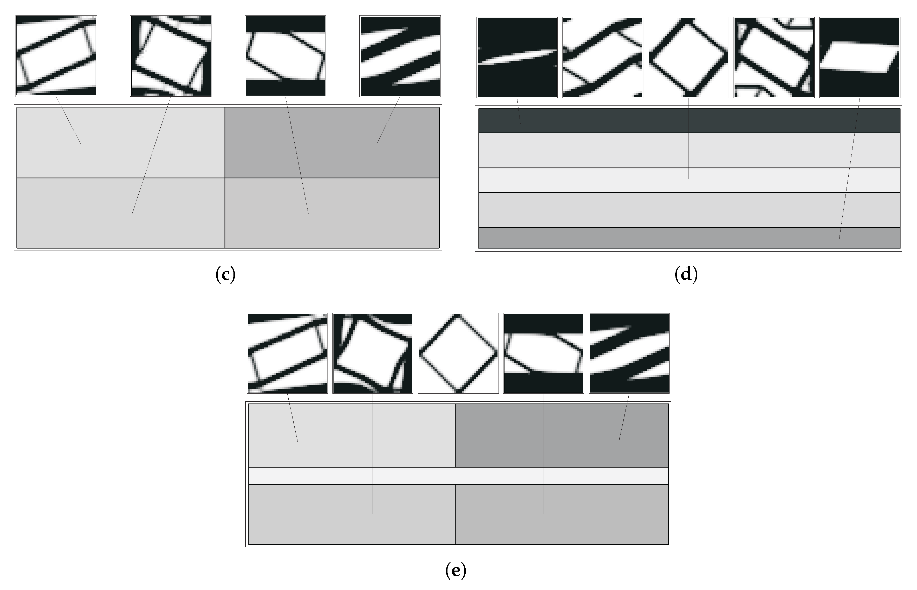
The horizontal division examples were also solved in the same conditions but using a CONLIN implementation. The added stability of these methods for the use of local constraint Lagrange multipliers to control the macroscale problem is better for hierarchical problems. Figure 22 shows the objective curve evolution for these problems, as shown in Figure 17. It is noted that the added stability makes the initial convergence faster and more balanced between different numbers of subdomains. However, the same problems with the influence of the filtering of sensitivities tend to arise for the cases of fewer divisions. These slowly update the solution towards a laminate configuration. Figure 23 shows the local topologies and macroscale densities for these problems, as seen for MMA in Figure 20 and Figure 21. It is possible to see that the basic topologies are the same as before, but effectively better defined in this case. This was expected, since the better stability of CONLIN in terms of the local Lagrange multipliers lessens some of the oscillations between macroscale densities and microscale response described before. Even so, the differences are small, and it is shown that MMA is a valid method for these applications. However, it becomes less stable for a large number of local problems (e.g., hierarchical approach), creating further convergence problems. Over the remainder of this document, the problems are once again solved using MMA.

The H8 method, where the macroscale density is kept constant throughout all the domains (and, conversely, microscales are less prone to these stability issues). In this case, all the local problems are solved according to the global volume constraint and are not conditioned by the macroscale density evolution. Figure 24 shows the evolution of the objective functions with two horizontal and vertical divisions, for discretisations between M2 and M5, using the worst-case equivalent strain weighting. The horizontal cases show once again the gradual tendency to become laminar with the action of the sensitivity filtering. Also as before, this issue does not appear for more subdomain divisions. In addition, the equivalent stress weighting allows the control of this effect. For vertical divisions, in spite of the expected problems, the response is even better than for H7. Figure 25 compares the objective function evolutions for both cases, using the M4 mesh. While for the horizontal divisions, the results are basically the same, the vertical divisions for H7 are clearly worse. This is due to the macroscale density update, which tends to transfer material between domains, leading to deviations that usually carry some inertia in terms of correction because of the simultaneous update of macro- and microscale variables. This does not happen for H8 because of the constant macroscale topology. This is also why the H8 topologies tend to be better defined, as shown in Figure 26 (since macroscale density is constant for H8, subdomain colours in this case are used just for representation and have no physical meaning). In H8, a better comparison with previous examples shows topologies obtained with an equivalent stress weighting. Furthermore, H8 tends to be faster and overall more stable than H7, leading to better results. In fact, in spite of H7 allowing, in theory, to achieve better results because of greater freedom in the material distribution, the gains are usually small in comparison with the greater dependency on processing parameters. Moreover, the practical approach tends to be closer to a lower dispersion of the volume fraction between constituent materials.

Just as a final example, these strategies are applied to a 3D problem. The microstructure mesh uses $30\times 30\times 30$ linear hexahedral elements. The H5, H6, H7, and H8 strategies are used, with the basis volume average weighting and SIMP, using $f_{\mathrm{v}}=0.5$ volume constraints. The linear elasticity problem is illustrated in Figure 27. Bending and torsion are applied to a cantilever I-beam. These loadings can be applied at once or used as multiload cases (ML) for optimisation. Examples are also shown with domain divisions for two and three subdomains for the H7 and H8 methodologies (vd. Figure 27d,e).

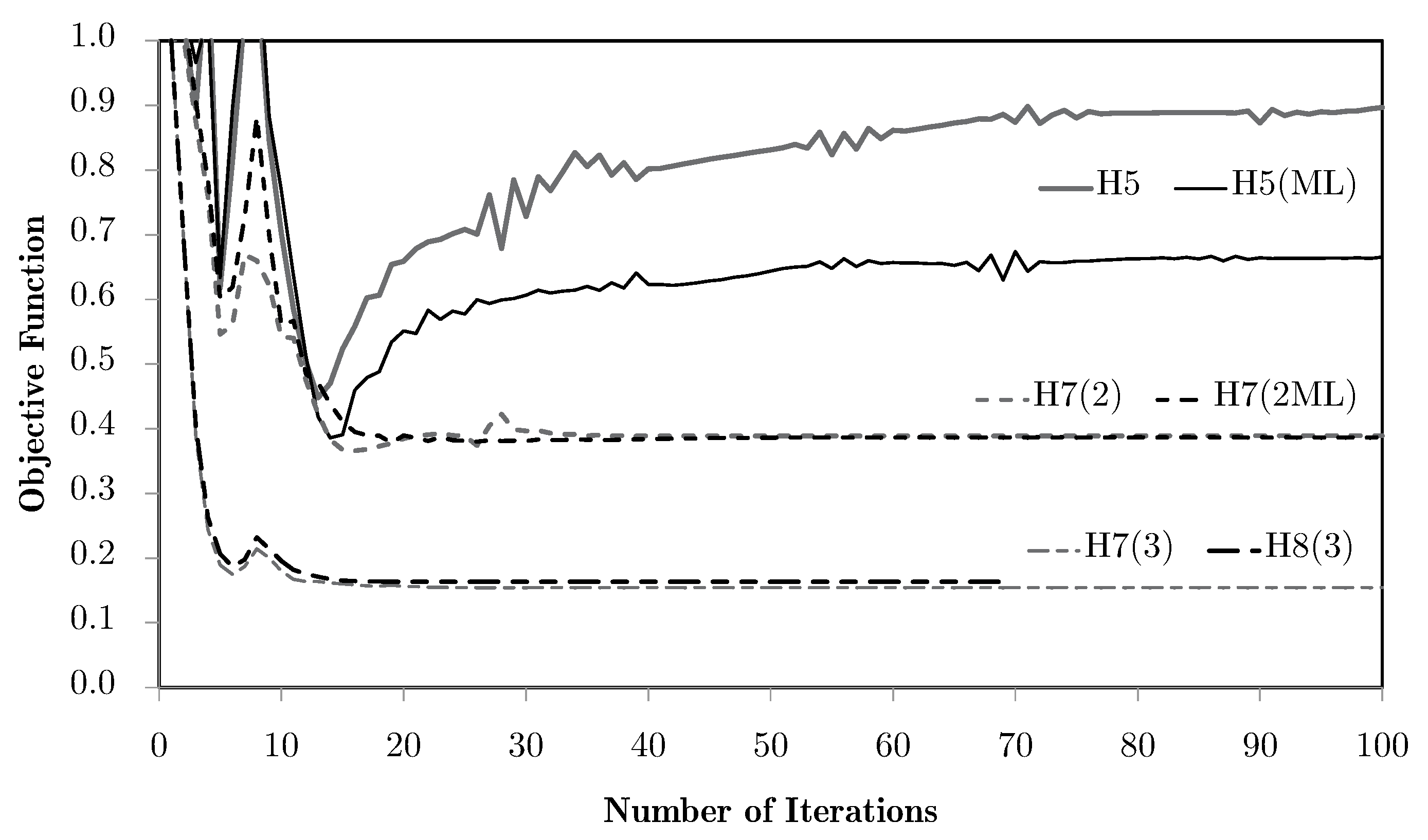
The objective function evolutions for different examples are shown in Figure 28. The behaviour is coherent with the one observed for 2D problems. There is an effective reduction in the objective function (minimisation of the strain energy), but with some instability for H5. In this case, the reduction is low when compared to the initial solution, moreover, in the case of simultaneous loading. The initial evolution is very similar between the cases of one and two local problems. Before the objective function starts rising again, there are some intermediate densities that keep the material phases connected, before they start becoming separated and the transversal stiffness decays. For multiple subdomains this does not happen, since there are at least two local problems that allow for a better material distribution and effective response. This is even more noticeable for three domains, where the response is much better. Note that in this case, the division was made with an engineering sense of flange regions for compression and tension, and the web region for shear resistance. Also note that, like before, the H8 solution is close to H7 while converging faster with a better topology definition.

The 3D cantilever I-beam example illustrates not only computational feasibility but also engineering insight. Subdomain divisions aligned with functional regions (flanges for bending, web for shear) produce more efficient material layouts, reflecting classical design practice in steel and composite beams. This shows that the method does not merely reduce computational cost but also provides guidance consistent with engineering intuition. The comparison between H7 and H8 in 3D further confirms that while H7 offers more freedom, H8 delivers faster convergence and more stable topologies. Topologies are shown in Figure 29 and Figure 30, for the use of H5 and H7/8 methodologies, respectively. The local problem topologies for H5 tend to approach laminates with the influence of the bending problem (vd. Figure 29e). Additional detail follows the inclusion of the torsion loading (vd. Figure 29f). This problem tends to create some instabilities, even becoming difficult to solve independently, even in the case of simultaneous loading (vd. Figure 29b), such as reaching a solution that is less stiff than some intermediate topologies (vd. Figure 29c). These are, however, characterised by some lack of definition because of intermediate densities. As these are penalised, the solution becomes more discrete but also less stiff. The use of alternative material combinations (e.g., $d_{\mathrm{m}}=0.05$), closer to the composite material approach, in turn, makes the topology more laminar, close to the bending response, and does not suffer from any of the problems seen before (vd. Figure 29g). For the multidomain optimisation, topologies are shown in Figure 30. All of these give a response better than the single domain solutions. However, the H7 solutions can suffer from some lack of definition as seen before (vd. Figure 30b), but only when MMA is used in both scales. Using CONLIN on the microscale, for instance, makes the local problems more stable. The three subdomain responses, instead, are shown to be good results and are close between H7 and H8. H7 gives a slightly better response because of the material transfer between local problems and macroscale density variation, but, as before, this is compensated by the greater stability and definition of the H8 approach. Overall, the 3D results are shown to be consistent with the overall analysis for 2D.

6. Final Remarks

The hierarchical topology optimisation problem presents some limitations regarding its practical application in structural optimisation [26]. To align this methodology more closely with the production of engineering materials, particularly composites and cellular structures, alternative numerical strategies were developed. These allow the optimisation of microstructural material topologies so that periodic distributions can be tailored to specific structural requirements. Other strategies introduce a predefined number of subdomains, producing solutions consistent with engineering practice, where different regions of a structure can be assigned different microstructures.

The examples presented in this work focus deliberately on standard benchmark problems. Even in these worst-case scenarios, the proposed methods demonstrate stable convergence, clear material layouts, and results compatible with manufacturing practice. In addition to these practical advantages, the subdomain strategies provide significant computational savings. By controlling the number of local problems, they enable finer structural detail without the prohibitive cost of fully hierarchical approaches.

When compared to other multiscale optimisation strategies in the literature, the subdomain method represents an intermediate path. It combines the conceptual simplicity of inverse homogenisation with the generality of full hierarchical approaches while drastically reducing computational effort. In this sense, it provides a practical compromise between fidelity and efficiency, well suited to design-oriented applications.

Limitations and Future Work. While the subdomain approach provides clear computational and practical advantages, some limitations remain. The effectiveness of the method depends strongly on subdomain selection. Poorly chosen divisions may dilute the optimisation effect, particularly when stress fields are highly localised. Automatic subdivision strategies, e.g., based on principal stress fields, should therefore be further developed. Also, manufacturing constraints were not explicitly included in this implementation. Nevertheless, the subdomain formulation is compatible with their integration. Feature-size filters commonly applied in SIMP-based methods [24] can be enforced at the subdomain level, integrated into the sensitivity filtering used here, and anisotropy constraints can be aligned with selected stress fields to guide manufacturable layups. Finally, the validation scope has been limited to benchmark cases, such as MBB beams and a simplified 3D I-beam. These were selected because they represent stringent test cases, but extension to more complex engineering structures and experimental validation is a natural next step. Such studies are expected to further demonstrate the method’s applicability, particularly for composite and cellular structures.

References

1. Bendsøe, M.; Kikuchi, N. Generating optimal topologies in structural design using a homogenization method. Comput. Methods Appl. Mech. Eng. 1988, 71, 197–224. [Google Scholar] [CrossRef]
2. Rodrigues, H.; Fernandes, P. A material based model for topology optimization of thermoelastic structures. Int. J. Numer. Methods Eng. 1995, 38, 1951–1965. [Google Scholar] [CrossRef]
3. Diaz, A.; Lipton, R. Optimal material layout for 3D elastic structures. Struct. Multidiscip. Optim. 1997, 13, 60–64. [Google Scholar] [CrossRef]
4. Theocaris, P.; Stavroulakis, G. Multilevel optimal design of composite structures including materials with negative Poisson’s ratio. Struct. Multidiscip. Optim. 1998, 15, 8–15. [Google Scholar] [CrossRef]
5. Hassani, B.; Hinton, E. Homogenization and Structural Topology Optimization: Theory, Practice, and Software; Springer: London, UK, 1999. [Google Scholar]
6. Theocaris, P.; Stavroulakis, G. Optimal material design in composites: An iterative approach based on homogenized cells. Comput. Methods Appl. Mech. Eng. 1999, 169, 31–42. [Google Scholar] [CrossRef]
7. Allaire, G. Shape Optimization by the Homogenization Method; Applied Mathematical Sciences; Springer: New York, NY, USA, 2002; Volume 164. [Google Scholar]
8. Rodrigues, H.; Guedes, J.; Bendsøe, M. Hierarchical optimization of material and structure. Struct. Multidiscip. Optim. 2002, 24, 1–10. [Google Scholar] [CrossRef]
9. Bendsøe, M.; Sigmund, O. Topology Optimization: Theory, Methods, and Applications; Springer: Berlin/Heidelberg, Germany, 2003. [Google Scholar]
10. Guedes, J.; Lubrano, E.; Rodrigues, H.; Turteltaub, S. Hierarchical optimization of material and structure for thermal transient problems. In IUTAM Symposium on Topological Design Optimization of Structures, Machines and Materials—Solid Mechanics and Its Applications; Bendsøe, M.P., Olhoff, N., Sigmund, O., Eds.; Springer: Berlin/Heidelberg, Germany, 2006; Volume 137, pp. 527–536. [Google Scholar]
11. Rodrigues, H. Topology optimization of structures: Applications in the simulation and design of cellular materials. In Computational Methods in Engineering & Science: Proceedings of Enhancement and Promotion of Computational Methods in Engineering and Science X, Sanya, China, 21–23 August 2006; Yao, Z.H., Yuan, M.W., Eds.; Springer: Berlin/Heidelberg, Germany, 2006. [Google Scholar]
12. Coelho, P.; Fernandes, P.; Cardoso, J.; Guedes, J.; Rodrigues, H. Hierarchical topology optimisation of structures subjected to constraints on material design. In Proceedings of the EngOpt2008—International Conference on Engineering Optimisation, Rio de Janeiro, Brazil, 1–5 June 2008. [Google Scholar]
13. Coelho, P.; Fernandes, P.; Guedes, J.; Rodrigues, H. A hierarchical model for concurrent material and topology optimisation of three-dimensional structures. Struct. Multidiscip. Optim. 2008, 35, 107–115. [Google Scholar] [CrossRef]
14. Gu, X.; He, S.; Dong, Y.; Song, T. An improved ordered SIMP approach for multiscale concurrent topology optimization with multiple microstructures. Compos. Struct. 2022, 287, 115363. [Google Scholar] [CrossRef]
15. Gao, J.; Wen, Z.; Zhai, X.; Chen, F.; Kang, H. Concurrent topology optimization of multiscalecomposites with differentiable microstructures. Comput. Methods Appl. Mech. Eng. 2024, 431, 117271. [Google Scholar] [CrossRef]
16. Dias-de-Oliveira, J. Topology Optimisation Methodologies for Structural Analysis. Ph.D. Thesis, Universidade de Aveiro, Aveiro, Portugal, 2013. (In Portuguese). [Google Scholar]
17. Dias-de-Oliveira, J.; Pinho-da-Cruz, J.; Teixeira-Dias, F. Domain-oriented multiscale optimization for composite materials. In Proceedings of the ESAFORM 25, 28th International ESAFORM Conference on Material Forming, Paestum, Italy, 7–9 May 2025; pp. 486–495. [Google Scholar]
18. Svanberg, K. The method of moving asymptotes—A new method for structural optimization. Int. J. Numer. Methods Eng. 1987, 24, 359–373. [Google Scholar] [CrossRef]
19. Fleury, C.; Braibant, V. Structural optimization: A new dual method using mixed variables. Int. J. Numer. Methods Eng. 1986, 23, 409–428. [Google Scholar] [CrossRef]
20. Fleury, C. CONLIN: An efficient dual optimizer based on convex approximation concepts. Struct. Multidiscip. Optim. 1989, 1, 81–89. [Google Scholar] [CrossRef]
21. Sigmund, O.; Petersson, J. Numerical instabilities in topology optimization: A survey on procedures dealing with checkerboards, mesh-dependencies and local minima. Struct. Optim. 1998, 16, 68–75. [Google Scholar] [CrossRef]
22. Rozvany, G.; Zhou, M.; Birker, T. Generalized shape optimization without homogenization. Struct. Multidiscip. Optim. 1992, 4, 250–252. [Google Scholar] [CrossRef]
23. Bendsøe, M.; Sigmund, O. Material interpolation schemes in topology optimization. Arch. Appl. Mech. 1999, 69, 635–654. [Google Scholar] [CrossRef]
24. Sigmund, O. Morphology-based black and white filters for topology optimization. Struct. Multidiscip. Optim. 2007, 33, 401–424. [Google Scholar] [CrossRef]
25. Coelho, P. Modelos Hierárquicos para a Análise e Síntese de Estruturas e Materiais com Aplicações à Remodelação Óssea. Ph.D. Thesis, Universidade Nova de Lisboa, Lisbon, Portugal, 2009. (In Portuguese). [Google Scholar]
26. Bendsøe, M. Optimization of Structural Topology, Shape, and Material; Springer: Berlin, Germany, 1995. [Google Scholar]
27. Guedes, J.; Kikuchi, N. Preprocessing and postprocessing for materials based on the homogenization method with adaptive finite element methods. Comput. Methods Appl. Mech. Eng. 1990, 83, 143–198. [Google Scholar] [CrossRef]
28. Pinho-da-Cruz, J.; Oliveira, J.; Teixeira-Dias, F. Asymptotic homogenisation in linear elasticity. Part I: Mathematical formulation and finite element modelling. Comput. Mater. Sci. 2009, 45, 1073–1080. [Google Scholar] [CrossRef]
29. Oliveira, J.; Pinho-da-Cruz, J.; Teixeira-Dias, F. Asymptotic homogenisation in linear elasticity. Part II: Finite element procedures and multiscale applications. Comput. Mater. Sci. 2009, 45, 1081–1096. [Google Scholar] [CrossRef]
30. de Kruijf, N.; Zhou, S.; Li, Q.; Mai, Y. Topological design of structures and composite materials with multiobjectives. Int. J. Solids Struct. 2007, 44, 7092–7109. [Google Scholar] [CrossRef]
31. Cherkaev, A.; Krog, L.; Küçük, I. Stable optimal design of two-dimensional elastic structures. Control Cybern. 1998, 27, 265–282. [Google Scholar]
32. Rodrigues, H.; Jacobs, C.; Guedes, J.; Bendsøe, M. Global and local material optimization models applied to anisotropic bone adaptation. In IUTAM Symposium on Synthesis in Bio Solid Mechanics—Solid Mechanics and Its Applications; Pedersen, P., Bendsøe, M.P., Eds.; Kluwer Academic Publishers: Dordrecht, The Netherlands, 1999; Volume 69, pp. 209–220. [Google Scholar]
33. Coelho, P.; Fernandes, P.; Rodrigues, H. Numerical modeling of bone tissue adaptationt—A hierarchical approach for bone apparent density and trabecular structure. J. Biomech. 2009, 42, 830–837. [Google Scholar] [CrossRef] [PubMed]
34. Rozvany, G. Exact analytical solutions for some popular benchmark problems in topology optimization. Struct. Multidiscip. Optim. 1998, 15, 42–48. [Google Scholar] [CrossRef]
Figure 1. Methodologies of multiscale topology optimisation: (a) simultaneous optimisation of both scales, (b) single microscale optimisation for a given macroscale application, and (c) subdomain multiscale optimisation.
Applsci 15 10201 g001
Figure 2. Influence of macroscale mesh refinement on problem size, using as a reference the number of local finite element systems to solve, comparing full hierarchical problems with examples of a single domain and 5 subdomains.
Applsci 15 10201 g002
Figure 3. Topology optimisation load cases (loads and supports): (a) bending, (b) shear, and (c) tension.
Applsci 15 10201 g003
Figure 4. Full hierarchical bending solution for a macroscale of  15 × 5  elements, resulting in 75 local problems to solve in spite of a very coarse macrostructure.
Applsci 15 10201 g004
Figure 5. Objective function evolution, using the H4 and H5 methodologies, for the test problems with the M5 mesh.
Applsci 15 10201 g005
Figure 6. Local topologies for the test loading cases: (a) compression, (b) tension, (c) shear, and (d) bending.
Applsci 15 10201 g006
Figure 7. Objective function evolution for the bending problem with different macroscale meshes.
Applsci 15 10201 g007
Figure 8. Objective function evolution for the bending problem with different weighting options and the M5 mesh.
Applsci 15 10201 g008
Figure 9. Topologies and anisotropy plots (Young’s modulus) for different microstructures calculated with an H5 methodology with different loads and parameters: (a) (1) shear, (2) compression, (3) bending, (b) (4) bending with equivalent strain weighting, (5) bending with equivalent stress weighting, (c) (6) bending with principal stress  σ 1  weighting (intermediate iteration), (7) bending with principal stress  σ 1  weighting, (d) (8) bending with principal stress  σ 2  weighting (intermediate iteration), and (9) bending with principal stress  σ 2  weighting (maximum radius of plots  r = ρ E 0 ).
Applsci 15 10201 g009
Figure 10. Topologies and anisotropy plots (Young’s modulus) for different microstructures calculated with an H5 methodology with different loads and parameters, with  d m = 0 , 1 : (1) shear with equivalent strain weighting, (2) bending with equivalent strain weighting, (3) tension with equivalent strain weighting, and (4) bending with principal stress  σ 1  weighting (maximum radius of plots  r = ρ E 0 ).
Applsci 15 10201 g010
Figure 11. Evolution of the objective function for different loads (shear and bending), using weighting with equivalent strains and principal stress  σ 1 .
Applsci 15 10201 g011
Figure 12. Optimal local topologies for different microscale mesh refinement levels: (ac 20 × 20  and (df 60 × 60  finite elements, for (a,d) shear, (b,e) bending, and (c,f) tension problems.
Applsci 15 10201 g012
Figure 13. Alternative test horizontal (#h) and vertical (#v) domain divisions for multiscale modes H7/8: (a) 2h, (b) 3h, (c) 4h, (d) 5h, (e) 5b, (f) 2v, and (g) 3v.
Applsci 15 10201 g013
Figure 14. Evolution of objective functions in subdomain multiscale topology optimisation H7, for a bending problem with two horizontal subdomains and equivalent strain weighting using macroscale meshes M2 through to M5.
Applsci 15 10201 g014
Figure 15. Evolution of objective functions in subdomain multiscale topology optimisation H7, for a bending problem with two vertical subdomains and equivalent strain weighting using macroscale meshes M2 through to M5.
Applsci 15 10201 g015
Figure 16. Example of (a) automatic subdivision in 5 domains using principal stress  σ 1  values, with (b) distribution of macroscale density and corresponding microscale topologies (grey levels represent macroscale density for H7 problems).
Applsci 15 10201 g016
Figure 17. Evolution of objective functions in subdomain multiscale topology optimisation H7, for a bending problem with different horizontal subdomain divisions and equivalent strain weighting using the M4 macroscale mesh.
Applsci 15 10201 g017
Figure 18. Evolution of the Lagrange multipliers of the local volume constraints,  λ , in a H7 multiscale optimisation ending problem with equivalent strain weighting, for the M4 macrostructural mesh.
Applsci 15 10201 g018
Figure 19. Evolution of objective functions in subdomain multiscale topology optimisation H7, for a bending problem with two horizontal subdomains and equivalent strain or stress weighting using the M4 macroscale mesh.
Applsci 15 10201 g019
Figure 20. Optimal topologies for a subdomain multiscale optimisation (H7) bending problem with (a,b) 2, (c,d) 3, and (e) 4 macroscale domain divisions (grey levels represent macroscale density for H7 problems).
Applsci 15 10201 g020
Figure 21. Optimal topologies for a subdomain multiscale optimisation (H7) bending problem with five (a) horizontal or (b) mixed macroscale domain divisions (grey levels represent macroscale density for H7 problems).
Applsci 15 10201 g021
Figure 22. Evolution of objective functions in subdomain multiscale topology optimisation H7 optimised with the CONLIN method, for a bending problem with different horizontal and subdomain divisions and equivalent strain weighting using the M4 macroscale mesh.
Applsci 15 10201 g022
Figure 23. Optimal topologies for a subdomain multiscale optimisation (H7) bending problem with (a) 2, (b) 3, (c) 4 and (d,e) 5 macroscale domain divisions solved with CONLIN (grey levels represent macroscale density for H7 problems).
Applsci 15 10201 g023aApplsci 15 10201 g023b
Figure 24. Evolution of the objective functions on the subdomain (H8) multiscale optimisation bending problem with two vertical and horizontal domains, using equivalent strain weighting and meshes from M2 to M5.
Applsci 15 10201 g024
Figure 25. Comparison between the H7 and H8 modes in the evolution of the objective functions on the subdomain (H8) multiscale optimisation bending problem with four vertical and horizontal domains, using equivalent strain weighting and a macrostructural mesh M4.
Applsci 15 10201 g025
Figure 26. Optimal topologies for a subdomain multiscale optimisation (H8) bending problem with (a,b) 2 and (c,d) 3 macroscale domain divisions.
Applsci 15 10201 g026
Figure 27. Definition of a 3D (a) bending and torsion problem of a cantilever I-beam with the deformed state for the (b) bending and (c) torsion cases, as well as (d) 2 and (e) 3 divisions for multiscale subdomain optimisation.
Applsci 15 10201 g027
Figure 28. Evolution of objective functions for a cantilever I-beam problem with bending and torsion applied simultaneously and as multiload cases (ML), using the H5, H7, and H8 methodologies (1, 2, and 3 domains).
Applsci 15 10201 g028
Figure 29. Local optimal topologies for a cantilever I-beam problem using an H5 methodology: (a) orientation reference, (b) simultaneous loading case, (c) intermediate solution of the simultaneous loading case, (d) multiload case (same weight), isolated solution for the (e) bending and (f) torsion problems, and (g) the solution for  d m = 0.05 .
Applsci 15 10201 g029
Figure 30. Local optimal topologies for a cantilever I-beam problem using a subdomain multiscale methodology: (a) H7 with two domains, (b) H7 multiload with two domains, (c) H7 with three domains (grey levels represent macroscale density for H7 problems), and (d) H8 with three domains.
Applsci 15 10201 g030