Abstract
Fault identification in Printed Circuit Board Assembly (PCBA) testing is essential for assuring product quality; nevertheless, conventional methods still have difficulties due to the lack of labeled faulty data and the “black box” nature of advanced models. This study introduces a label-free, interpretable self-supervised framework that uses two pretext tasks: (i) an autoencoder (reconstruction error and two latent features) and (ii) isolation forest (faulty score) to form a four-dimensional representation of each test sequence. A two-component Gaussian Mixture Model is used, and the samples are clustered into normal and fault groups. The decision is explained with cluster mean differences, SHAP (LinearSHAP or LinearExplainer on a logistic-regression surrogate), and a shallow decision tree that generated if–then rules. On real PCBA data, internal indices showed compact and well-separated clusters (Silhouette 0.85, Calinski–Harabasz 50,344.19, Davies–Bouldin 0.39), external metrics were high (ARI 0.72; NMI 0.59; Fowlkes–Mallows 0.98), and the clustered result used as a fault predictor reached 0.98 accuracy, 0.98 precision, and 0.99 recall. Explanations show that the IForest score and reconstruction error drive most decisions, causing simple thresholds that can guide inspection. An ablation without the self-supervised tasks results in degraded clustering quality. The proposed approach offers accurate, label-free fault prediction with transparent reasoning and is suitable for deployment in industrial test lines.
1. Introduction
Printed Circuit Board Assembly (PCBA) testing is a crucial phase in electronics manufacturing, ensuring product quality and reliability. Any defect or failure in PCB fabrication not only compromises the functionality of the final product but also leads to significant financial losses due to scrap, rework, and delivery delays [1]. However, traditional fault detection methods typically rely on full or semi-supervised learning with abundant labeled data, which is often impractical in manufacturing settings because labeled fault samples are limited and failures are rare and diverse in nature [2,3].
Self-supervised learning (SSL) has emerged as a possible approach to tackle these difficulties by deriving useful feature representations from unlabeled data [4]. In SSL, models learn on pretext tasks that are not the main goal, which allows extracting meaningful representations of data and understanding the underlying structure without any help from any kind of supervised task [4]. Here, the representations learned through pretext tasks can be applied to specific tasks, such as fault prediction. This method is suitable for PCBA testing, which is characterized by an abundance of test data but a lack of labeled faults or dependence on binary, rule-based solutions. Interpretability is another important factor in practical failure prediction systems. Advanced machine learning models often act as “black box” models, making it difficult to understand how they make decisions or what features differentiate a fault from normal conditions. In manufacturing contexts, a model that predicts a fault without explanation may be of limited use [5,6]. Improving interpretability is essential to build trust in SSL-based fault prediction. The interpretability goal here is to expose which learned signals and pretext outputs drive the clustering and the fault decision, so an AI developer can debug, validate, and deploy the pipeline. Mapping those signals to electrical root causes for engineers is planned as future work.
This paper presents an innovative framework for fault prediction in PCBA testing, utilizing SSL to address existing challenges. The primary objective is to utilize self-supervised representation learning with unlabeled PCBA test sequences, while incorporating approaches that enhance the interpretability of the results. The primary goal of this research is to create a fault prediction system that can operate without the need for labeled data, providing meaningful insight alongside its predictions, and adapting to the dynamic and complex nature of PCBA test environments. This is achieved by developing a framework that uses dual pretext tasks to obtain strong representations from test signals, finds possible faults on its own, and gives explicit explanations of what affects each prediction. The key contributions of this study are as follows:
- Dual Pretext Task for Robust Representation Learning: A dual pretext learning methodology to enhance self-supervised representation learning, promoting the creation of more advanced and adaptable features, hence improving fault detection capabilities across many contexts.
- Interpretability-Driven Fault Characterization: Introducing an interpretability analysis module to fault characterization to address the “black box” issue of SSL models for verifying model decisions and identifying the root causes of failures.
- Empirical Validation on Real-World PCBA Data: Tested on real-world PCBA data and demonstrated superior fault detection performance of proposed frameworks relative to traditional methodologies, including agglomerative and k-means clustering models, both with and without the inclusion of two pretext tasks.
The state of the art is advanced in PCBA testing by addressing two major challenges: (1) the lack of labeled faulty data and (2) the need for trustworthy, interpretable models in industrial settings. By combining an SSL framework with explainability, this research opens the door to scalable, human-centric AI solutions in electronics manufacturing. This paper is structured as follows: Section 2 reviews the current literature, Section 3 outlines the materials used and the experimental methods employed, Section 4 shows and discusses the experimental findings, Section 5 explains the significance of these results and their impact on PCBA testing, and Section 6 highlights the key contributions of the study and suggests directions for future research.
2. Related Work
Early research on fault prediction in Printed Circuit Board (PCB) and PCBA lines has been dominated by fully supervised computer vision frameworks [7,8,9,10,11,12,13]. All of them relied on many labeled faulty images, which are limited in real scenarios. Although these studies confirm that deep models can exceed traditional rule-based optical inspection, they remain image-centred and do not address the mixed-signal numeric parameters produced by in-circuit or functional test equipment such as an embedded test system (ETS).
Unsupervised methods like one-class autoencoders, principal-component monitoring, and isolation forest (IForest) have grown more relevant in this domain because it is hard to obtain enough labeled data [14]. Autoencoders compress data samples and can identify faults by producing a high reconstruction error for those faulty samples. However, there is a risk of overfitting, especially when the latent dimension is large or when normal data has a more discrete distribution [15]. On the other hand, IForest tackles high-dimensional data by breaking down the feature space in a recursive manner, using shorter average path lengths to assign a fault score without relying on density estimation [16]. A recent survey has pointed out that many traditional unsupervised detectors struggle with highly non-linear data, suggesting that SSl might provide a better solution [17].
Beyond classic unsupervised detectors, non-negative matrix factorization (NMF) offers meaningful, part-based decompositions for industrial monitoring. A recent approach, graph-regularized orthogonal NMF with Itakura–Saito divergence (GONMF-IS), focuses on fault detection in complex, non-Gaussian processes [18]. It combines IS divergence for better modeling of heavy-tailed data, graph regularization to maintain local structure, and orthogonality constraints for improved factor separability and interpretability. This method outperforms traditional NMF variants, highlighting the importance of topology-aware regularization and non-Euclidean divergences in industry [18]. While NMF emphasizes low-rank additive structures, the label-free SSL framework focuses on reconstruction error and isolation scores, using a probabilistic clustering method. Both approaches are unsupervised and interpretable but rely on different inductive biases, making them potentially complementary for PCBA testing.
SSL has recently appeared as a nice alternative between fully unsupervised and fully label-dependent supervised methods. A one-dimensional convolutional neural network (1DCNN) with time-series data augmentation was used to generate pseudo-labels and learn normal data characteristics, achieving high accuracy and efficiency in detecting anomalies, and still has limitations in generalizing to highly variable or multi-seasonal time-series data and explainability [19]. A novel self-supervised learning framework was introduced to enhance the detection of solder joint defects in PCBs, addressing significant data imbalance by effectively learning robust representations from unlabeled data, and has dependency on labeled data for fine-tuning and sensitivity to augmentations [20]. SPT-AD suggests a self-supervised pyramidal Transformer model that makes it easier to find anomalies in bearing vibration data [21]. However, it has some limitations in terms of generalization, as it relies on synthetic anomalies, loses information during compression, is only tested in controlled, single-dataset settings, and lacks clear interpretations. In the PCB domain, SLLIP has already demonstrated the benefit of SSL features over raw pixels [10]. Beyond computer vision, a recent time-series review summarized how contrastive and predictive pretext tasks improve vibration-based fault detection for rotating machinery, yet reported that interpretability remains absent mainly in the SSL framework [22,23]. Overall, the literature confirms the effectiveness of SSL for fault detection, but still found two gaps: (i) limited investigation on numeric PCBA test sequences, and (ii) inadequate attention to model transparency or trustworthiness.
Explainable AI (XAI) techniques, such as Shapley Additive explanations (SHAP), have been introduced to identify feature importance in machine learning applications [24]. In bearing-health studies, key vibration statistics were highlighted and accuracy above 98.5% was reported, with clear feature rankings [25]. A recent review reported that post-hoc feature attribution now dominates fault-diagnosis XAI, while global surrogates such as decision trees are used less [6]. Generic Shapley values were first applied to log-based fault detection, and the roles of features in tree models and DeepLog were revealed [26]. Temporal order was built into Shapley values by ShaTS for IIoT detectors [27]. Correlation-aware SHAP was introduced for industrial control systems to support root-cause search when signals are dependent [28]. Context-focused SHAP filtering was used to reduce noise when explaining energy-use faults in buildings [29]. SHAP was also combined with clustering to derive simple decision rules for semiconductor equipment failures, so cluster outputs could be mapped to human-readable logic [30].
Prior research established that SSL can learn rich representations from unlabeled data and that XAI can improve trust in fault-diagnosis models. However, existing solutions either focus on optical PCB inspection or overlook interpretability when dealing with numeric test data. Furthermore, most clustering approaches rely on ’ad hoc’ heuristics to label the smallest group as faulty. To the best of our knowledge, no previous work unifies dual SSL pretext tasks, probabilistic clustering, and post-hoc explanations for PCBA test sequences. Table 1 lists a narrow down summary of recent works.

Table 1.
Recent compact comparative studies.
The proposed framework, therefore, advances the state of the art by (i) extracting complementary reconstruction and isolation-based features without labels, (ii) clustering them with a soft-boundary GMM, and (iii) delivering transparent fault explanations via cluster mean, SHAP, and surrogate models.
3. Material and Method
3.1. Data Description
Data was extracted using the ETS shown in Figure 1, which automates the testing of PCBA units by capturing critical electrical parameters during a complete test sequence. Each entry in the dataset corresponds to a specific test result, identified by an ID number and a timestamp indicating when the test was performed. The execution time for each test was also recorded. In a single test sequence, five measurements are taken: the DCDC converter voltages (2 volts and 1 volt), the current measurement before flashing, the transmit current, and the sleep current. These five measurements are considered features for further processing within the test sequence. Although each unit contains five ETS measurements, instead of performing clustering in the original feature space, a compact and semantically meaningful four-dimensional joint representation is created. This new representation captures key aspects such as the difficulty of reconstructing the sample, the ease of isolating it using a tree ensemble, and two distinct directions of signal variation. This approach enhances interpretability and reduces dimensionality when compared to the raw data inputs [31]. The Figure 2 illustrates the overall workflow, where it starts through the collection and preprocessing of data, is processed within an SSL framework (using Autoencoder and Isolation Forest for joint feature representation and clustering), and is then evaluated through clustering performance and interpretability analysis to identify faulty PCBA.
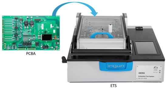
Figure 1.
ETS used for PCBA testing [32,33].
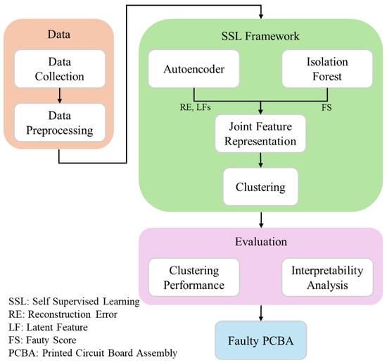
Figure 2.
Work flow diagram.
The ETS generates a straightforward outcome for each unit, assigning a label of either normal or fault. The testing engineer decides the limits for each test conducted on a single PCBA. If any measurement exceeds these limits, the unit is labeled as fault. These labels get automatically recorded during the testing process and stored in the production database. Although they are not used for training or selecting models, they play a role in calculating external validation metrics after clustering, especially in cases where setting limits may not be feasible. A total of 31,005 PCBAs were tested under consistent environmental conditions to ensure data reliability.
3.2. Data Preprocessing
Data preprocessing begins with the cleaning of the data to remove any unnecessary or irrelevant information [34]. Upon completion of the previous step, missing values are addressed to ensure the dataset is comprehensive. In order to effectively fill in gaps, forward and backward fill methods are utilized for this purpose [35]. After missing values are filled, all features are rescaled [36]. This is a necessary step to ensure that every feature contributes equally to our analysis. Rescaling plays a vital role for specific algorithms, such as clustering methods and autoencoders, which tend to be very sensitive to the scale of input features [37,38].
3.3. Self-Supervised Learning Framework
In the self-supervised learning (SSL) framework, two pretext tasks were designed to learn informative representations of the data without relying on labeled faults. The objective is to identify features that capture faults or deviations in the data distribution, which may indicate faulty PCBAs. The two unsupervised pretext tasks employed are (1) an autoencoder reconstruction task and (2) an IForest fault detection task. The outputs generated from these tasks include the reconstruction error from the autoencoder and a faulty score from the IForest, along with latent features that act as inputs for the final clustering stage. Since the percentage of faulty PCBs is unknown, it is not possible to predict faulty samples based solely on these two pretext tasks. By training these tasks on all data, the model learns the inherent structure of the test measurements in a self-supervised manner.
3.3.1. SSL Pretext Task 1: Autoencoder
To extract meaningful representations from the PCBA test results, an autoencoder is used to learn latent features. Autoencoders are widely used for fault detection by accurately reconstructing normal data and using the reconstruction error as an indicator of faults [39]. In our setup, a feed-forward autoencoder is implemented with an input layer consisting of 5 neurons. The encoder has two hidden layers that contain 4 and 3 neurons, respectively, and a latent code dimension of 2. The decoder is symmetric to the encoder, with hidden layers containing 3 and 4 neurons, and outputs a 5-dimensional reconstruction. All of the hidden layers use ReLU activation functions to assist the network learn complicated patterns. The 2D bottleneck layer and the last output layer, on the other hand, use linear activations, which means that values are not compressed or clipped. This keeps the entire range of outputs needed for regression. The Adam optimizer with a learning rate of 0.001 and mean squared error (MSE) as the loss function is used for training. The model trains for up to 500 epochs, using small batches of 32 samples each. To keep track of progress, 20% of the data is randomly set aside as a validation set every epoch. Training stops early if the validation MSE does not get better for 10 epochs in a row. To avoid overfitting, training finishes early if the validation MSE does not improve for 10 epochs in a row. The model reverts to the version with the highest validation score when this occurs. Data is shuffled before each epoch to ensure variety in training batches. No dropout or weight decay is used, as the model relies on early stopping and random validation splits to stay general. Table 2 shows the concise summary. To reduce the model’s variance, the autoencoder is kept intentionally compact and trained with early stopping using a separate validation set. The number of parameters is significantly lower than the amount of samples, creating a beneficial ratio of samples to parameters. Early stopping is applied to prevent overfitting [40]. During training, the autoencoder learns to minimize the MSE between input and reconstruction . The reconstruction error for a sample i is given by the MSE:
where is the jth feature of the ith instance and n is the number of features [41]. Because the autoencoder is trained mostly on normal data, it reconstructs normal patterns with a low error that is near zero. In contrast, when it encounters faults, the reconstruction error produces higher values [39]. The trained encoder provides a 2-dimensional latent vector for each instance, which captures the essential signal patterns. These latent features, along with the reconstruction error, serve as a pretext task for SSL to identify faults.
Table 2.
Autoencoder training parameters.
Figure 3 illustrates the reconstruction error values in the test instances, along with the distribution of these errors. In general, one could set a fault threshold on err_ae to identify faults. In our study, however, we do not directly set the threshold err_ae; instead, it is treated as one feature within the joint fault representation for further analysis. The plot shows the reconstruction error (err_ae) for each sample in the test set against the sample index. As expected, most samples show low reconstruction errors, indicating that the autoencoder effectively reconstructs normal patterns. However, a few samples display significantly higher errors, which likely indicate faults. The histogram highlights the density of errors across the range, with the majority clustering around zero and forming a sharp peak. This suggests that the autoencoder has learned to accurately reconstruct normal data. In our framework, err_ae is treated as one feature in the joint feature representation, contributing valuable information about the deviation of each instance from the learned normal behavior.
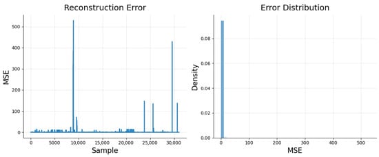
Figure 3.
Reconstruction error of autoencoder.
To ensure that the autoencoder can accurately identify normal patterns in the data, its training is closely examined. It is clear from the loss curve in Figure 4 that the autoencoder is successfully recreating normal data on the validation set because the MSE is near zero. It is clear that err_ae captures the fault well because the final reconstruction errors on the training data show a skewed distribution with a long tail.
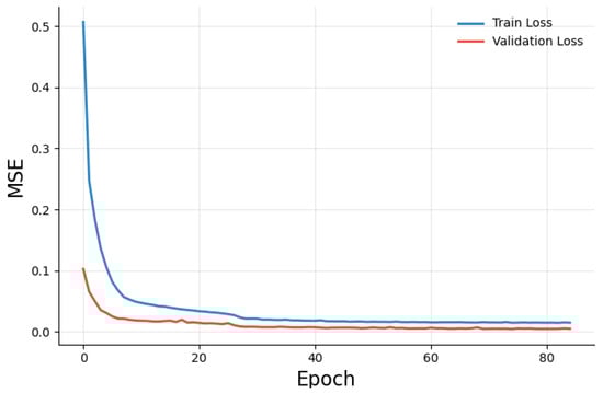
Figure 4.
Loss curve of autoencoder.
3.3.2. SSL Pretext Task 2: Isolation Forest Fault Score
In the second pretext task, an IForest algorithm is used to quantify the “faultiness” of each test sample via an unsupervised anomaly score. The IForest is an ensemble of random binary decision trees specialized for anomaly or fault detection [16]. It operates on the principle that anomalies such as faulty test instances are easier to isolate from the bulk of data than normal instances [16]. The forest was trained on the same set of 5-dimensional test feature vectors (with no labels) to build a model of the data’s standard patterns. For each sample, the trained IForest produces a faulty score (score_if) based on the average path length required to isolate that sample in the random trees. Formally, faulty samples tend to have shorter path lengths in isolation trees (they get isolated quickly by random splits), resulting in higher faulty scores after normalization. The IForest does not require any fault labels, it purely depends on the data distribution. A high score_if indicates the sample is likely to be a fault, whereas a low score means the sample is in a dense region of a distribution that is likely to be normal.
Figure 5 illustrates the faulty scores for all instances. The graph illustrates the faulty scores for each sample plotted in relation to their respective indices. As expected, the majority of normal instances tend to receive low scores, whereas the faulty instances are likely to show considerably higher values. In this step, no strict cutoff for was established to identify faults, since a predetermined threshold was not available. Instead, the score is integrated into the joint feature representation for the final decision, like err_ae.
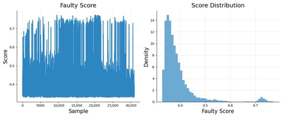
Figure 5.
Faulty score of isolation forest.
3.4. Joint Feature Representation
After calculating the autoencoder reconstruction error and the faulty score for each instance, a joint feature representation is obtained that combines all the relevant information. From Pretext Task 1 (autoencoder), each sample’s reconstruction error is retained err_ae as a feature, along with the two latent variables from the bottleneck layer (z_ae_1, z_ae_2). From Pretext Task 2 (IForest), the score_if is acquired for each sample. These four features are then concatenated to form a new feature vector:
The motivation is that err_ae and score_if capture complementary aspects of abnormality, specifically reconstruction difficulty and isolation rarity, while (z_ae_1, z_ae_2) offers a compressed summary of the original test measurements of PCBA testing. By combining these features, a feature space is formed where faulty PCBAs are more distinguishable from normal PCBAs [31]. This method of generating new feature representations through self-supervised pretext tasks is essential, as directly clustering the high-dimensional raw measurements would not be a good alternative.
3.5. Clustering Using Gaussian Mixture Model
A Gaussian Mixture Model (GMM) clustering algorithm is employed on the joint feature vectors to predict the fault. The GMM is a probabilistic clustering model that assumes the data is generated from a mixture of Gaussian distributions [42]. In order to classify the data into two groups, one for normal instances and another for faults, the number of mixture components is set at K = 2 with full covariance matrices. K-means is also used for initialization in order to assign starting tasks. Every cluster k has a mixture weight , a covariance matrix , and a mean vector (centroid) in the four-dimensional feature space [42]. The underlying assumption is that normal data points cluster around a different mean than anomalous samples in this joint feature space. After training the GMM on all , each instance obtains a posterior probability of belonging to each cluster. Each instance is assigned to the cluster with the highest posterior probability. A binary clustering of the data is produced. One cluster is then identified as the “normal” group, while the other is the “fault” group. To determine which cluster is a fault, its centroid characteristics, and relative sizes are analyzed [43]. Typically, the fault cluster is expected to be smaller (since faults are rare) and to have a higher mean reconstruction error and IForest score. Indeed, in our experiments, the cluster with a higher average err_ae and score_if corresponded to the known faults. This approach effectively gives a binary labeling of each test instance: normal or faulty, which is derived in an unsupervised manner.
3.6. Evaluation
3.6.1. Clustering Performence
To ensure the clustering is accurate, both internal and external validation are performed. Internal validation involves using unsupervised metrics to examine the clustering structure, while external validation involves comparing clusters to factory normal/fault labels for analysis. The clusters are correctly formed in the process of internal validation by observing how well they separate from one another and how well they stick to one another. In contrast, external metrics provide an objective measure of the cluster’s agreement with the real faulty PCBA results, but they are not used for training or adjusting the model. The Calinski–Harabasz Index, the Davies–Bouldin Index, and the Silhouette Coefficient represent three standard internal clustering indices that have been computed [44]. The clustering performance is subsequently evaluated by using the known status labels (fault/normal) of PCBA for each test result, even though clustering is an unsupervised process. The Adjusted Rand Index (ARI), Normalized Mutual Information (NMI), and Fowlkes–Mallows Index (FMI) were also calculated as three common external cluster evaluation metrics [45]. This comprehensive evaluation framework ensures that our self-supervised fault detection model is not only accurate in identifying faulty PCBAs but also in forming meaningful clusters of PCBAs in the feature space.
3.6.2. Interpretability Analysis
To interpret the resulting clusters and understand the contributing features for fault detection, several analyses were performed on the trained GMM and the features.
To understand the contribution of each feature to the cluster separation, a surrogate logistic-regression model was also trained with the GMM predicted cluster labels and computed SHAP values using LinearSHAP (LinearExplainer) to quantify the importance of each feature. SHAP values provide a unified measure of feature importance by attributing the prediction for each sample to the input features based on their contribution, and also normalized into a summation of 1. This plot ranks the features based on their average absolute SHAP value across all samples, providing insights into which features are most influential in predicting the label for the PCBA test. Moreover, the overall SHAP variance is also computed to check the stability of feature importance across samples. These interpretable models serve as global surrogates to the black box GMM, allowing us to explain the clustering results in a transparent way.
The ability of each feature to distinguish between the two identified clusters was measured by comparing their distributions. For each input feature, the mean absolute difference between the averages of the two clusters is estimated using the following formula:
Features that showed a larger mean difference are considered more crucial in separating the clusters.
A small decision tree classifier (of depth 3) was trained as another surrogate to extract simple if–then rules, dividing the clusters. The feature space is partitioned into rectangular regions by thresholding features, giving an interpretable set of conditions for cluster-predicted labels. By fitting a decision tree on the cluster labels and then identifying rules, faulty PCBA is obtained. This tree was matched with the GMM clustering with high fidelity and provided a human-readable description of the boundary.
3.7. Ablation Study
To evaluate how effective the proposed methodology is, several ablation studies were carried out:
- Without Self-Supervised Learning: Clustering is performed directly on the raw rescaled features without including pretext tasks, such as autoencoder reconstruction error, latent features, and the IForest faulty score generation. The results are not promising when compared to the SSL pipeline, showing that SSL plays a crucial role in improving feature representation.
- Comparison with Other Clustering Algorithms: K-means clustering is applied to the joint feature set obtained by the pretext task. Although it produced fairly good results, GMM performed promisingly in both internal and external validation metrics. Agglomerative Clustering is also tested.
Throughout the methodology, various hyperparameters are fine-tuned to enhance performance. For the autoencoder, different network architectures are tested by changing the number of hidden neurons and the dimensions of the latent space. The results showed that a bottleneck size of 2 with a structure of offered a good balance between compression and reconstruction accuracy. These two-dimensional latent features are chosen because they encourage meaningful feature learning while still effectively reconstructing normal data.
In terms of the IForest model, important adjustments are made, particularly regarding the number of estimators or trees. An IForest with default hyperparameters is used. Additionally, the contamination parameter, indicating the expected fraction of faults, was set to “auto.” This means the identification of faults will not be restricted until the final evaluation stage.
To determine the best overall model, an ablation study that compared different variants of the pipeline was conducted. Specifically, a baseline approach is applied, where clustering is directly performed on the raw five-dimensional test measurements of each PCBA, without incorporating features from the pretext task. Additionally, other clustering methods are evaluated.
4. Results
4.1. Clustering Performance
The performance of the SSL-based framework for clustering was assessed using both internal and external validation metrics. Internally, the feature space created two different clusters, with the Silhouette Coefficient at 0.851. The Calinski–Harabasz Index was recorded as 50,344.195, while the Davies–Bouldin Index was 0.399, which indicates that the clusters are compact and well-separated. Table 3 shows the detailed performance metrics.
Table 3.
Performance metrics of GMM clustering.
On the external quality measure, the SSL model shows a strong alignment with known labels. The model achieved an ARI of 0.721, an NMI of 0.585, and a Fowlkes–Mallows FM score of 0.977. The values of ARI and Fowlkes-Mallows Index suggest that the GMM effectively categorized the data into “fault” and “normal” samples, closely matching the actual outcomes.
Figure 6 illustrates that the separation of faulty samples and normal samples is clear with PCA (3-component) visualization. One cluster, highlighted in blue, represents the normal PCBAs, while the smaller group, shown in red, corresponds to faulty PCBAs. There is a distinguishing boundary between these two clusters in the PCA plot, suggesting that the features extracted by the model successfully distinguish the faulty samples from the normal ones.
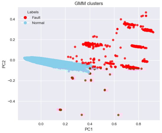
Figure 6.
PCA-based 2D visualization of clusters.
Figure 7 shows the PCA-based visualization from raw features with GMM labels. A tight blue group sits near the origin, while red points form a tall vertical band around PC1 (0), and several red faults lie far to the left on PC1. Overlap between the two groups is seen near the center, so the boundary is less distinct than in Figure 6. The PC1 indicates that the raw features dominate the first principal component. As a result, class separability is reduced, and GMM must partition the data with more mixing. This contrast indicates that joint features provide a more discriminative space for fault identification than raw inputs.
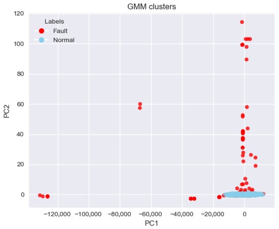
Figure 7.
PCA-based 2D visualization of clusters using raw features.
4.2. Interpretability Analysis
Two types of interpretive approaches are employed in explaining the clusters: (i) global feature importance and (ii) simple rule sets derived from a surrogate model. Figure 8 and Figure 9, along with Table 4, depict the results.
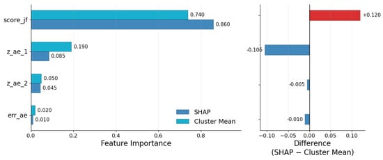
Figure 8.
Comparative feature importance (normalized): SHAP vs. cluster mean, the difference between SHAP and cluster mean.
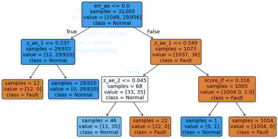
Figure 9.
Tree to understand if–then separation of GMM clustering.
Table 4.
Cluster means.
Global feature importance was assessed through two methods. The LinearSHAP feature importance was calculated using a logistic-regression surrogate model, which was trained to predict the GMM labels. The difference in cluster means was also calculated for each feature. The faulty score (score_if) is dominant in both analyses, with SHAP at and mean-difference at . The latent features (z_ae_1, z_ae_2) encompass the second and third positions, with values of SHAP and , respectively. The autoencoder reconstruction error (err_ae) is among the least significant features, as confirmed by both analyses. This aligns with expectations, given that a limited number of faulty PCBAs exhibit large errors, while the majority of normal PCBAs or samples remain close to zero. Figure 8 illustrates the changes in feature importance calculations: score_if , z_ae_1 , z_ae_2 , and err_ae . This pattern suggests that score_if accounts for the majority of decisions in faulty PCBA prediction.
Table 5 provides an overview of the unnormalized SHAP values for each input feature across different samples. The average SHAP values for all features are nearly zero, which indicates there is not a strong average influence from any single feature. However, the standard deviations (Std) reveal significant differences in how relevant each feature is to predictions. Among them, score_if shows the greatest variability with a standard deviation of 2.228, meaning its impact on model predictions varies greatly from sample to sample and can often be substantial. On the other hand, features like err_ae demonstrate very little variability (Std = 0.056), suggesting that they contribute minimally or serve a stabilizing effect within the model’s decisions. These findings point to score_if as the main factor driving prediction variability, even though its average effect is close to zero.
Table 5.
Overall (across-sample) statistics of SHAP values per feature.
The cluster means presented in Table 4 illustrate the feature-wise mean of two distinct distributions or clusters. A greater difference signifies enhanced separation and identifies the most significant feature. The clusters show a mean for score_if and , along with additional details provided in Table 4.
To extract the if–then rules that are displayed in Figure 9, a decision tree with a depth of three was fitted to the GMM labels. The root starts from err_ae. If , samples are normal for the majority. A small number of samples are fault when . Another small branch checks z_ae_2; many remain normal, while a small group is fault. If , samples are treated as fault. This branch is refined by . The region is dominated by the fault. A final check uses the IForest score, , which keeps the fault label in most cases. Only one sample changes to normal. A “faulty” PCBA is determined either by a significantly high faulty score or poor reconstruction from the autoencoder, or both. All of the rules that are derived from this decision tree are interpretable and intuitively sound, suggesting that this is the case. In order to effectively provide a practical framework for understanding the clustering, the surrogate tree establishes a minimal set of conditions. All the rules derived from this decision tree are interpretable and intuitively sound, confirming that a “faulty” PCBA is determined either by a significantly high faulty scor, poor reconstruction from the autoencoder, or both. The simple conditions established by the surrogate tree effectively provide a practical framework for understanding the clustering.
However, the three explanation methods analyzed in this study deliver consistent and complementary representations of the decision boundary. SHAP on the logistic-regression surrogate identifies the IForest fauty score as the top important feature, followed by two latent codes, and reconstruction error provides additional but relatively weaker evidence on average. The cluster mean differences are ordered in the same way as the effect sizes between clusters. The shallow decision tree turns this pattern into some simple threshold rules we can act upon during testing. Combined, SHAP provides both magnitude and direction at the global level, the mean-difference analysis provides separation in a model-agnostic manner, and the tree reveals human-readable cut-points that capture simple interactions. The slight differences between the three views are as expected, as they all optimize different aims (attribution, distributional separation, and rule fidelity), but the agreement on the primacy of the faulty score and significance of the autoencoder features works to raise confidence in the interpretation.
In all perspectives, score_if is the primary influential feature. The alignment among SHAP, cluster mean difference, and the tree rules reinforces the reliability of the explanation and the stability of the defined boundary between normal and faulty PCBA.
4.3. Ablation Study
An ablation study was performed to assess the effectiveness of the proposed SSL framework and the choice of clustering algorithm on overall performance. The results indicate the substantial benefits of SSL feature learning. Clustering quality significantly decreased when the SSL pretext task was skipped before having joint features, and clustering was conducted using simply the original test measurements, specifically the five-dimensional test signals, excluding reconstruction error or faulty scores. The quality of clustering significantly deteriorated.
This indicates that, in the absence of the enhanced feature space offered by SSL, unsupervised clustering faced challenges in properly grouping faulty boards, leading to associations with actual faults that were nearly random. The substantial drop in performance illustrates the critical role of the SSL framework. The pretext tasks effectively captured a representation that allowed for the natural distinction between faults and normal samples, while clustering based solely on raw inputs was unable to reliably identify faults.
The results presented in Table 6 indicate that k-means demonstrates superior performance compared to the other three algorithms, achieving a Silhouette score of 0.563, a Calinski–Harabasz Index of 23,600.533, and a Davies–Bouldin Index of 0.599. Agglomerative Clustering yields a Silhouette score of 0.553, a Calinski–Harabasz Index of 22,317.881, and a Davies–Bouldin Index of 0.594, indicating slightly lower performance compared to k-means, yet the results are closely aligned. GMM exhibits inferior performance, demonstrated by a Silhouette score of 0.329, a Calinski–Harabasz Index of 510.907, and a Davies–Bouldin Index of 2.610, which suggest significantly less coherent clustering. Without SSL, the direct unsupervised approach is significantly inadequate.
Table 6.
Comparison of clustering algorithms without pretext task.
Furthermore, comparisons were conducted between GMM and other common clustering algorithms with the identical SSL-generated features. K-means clustering in the four-dimensional feature space gave satisfactory results, yet consistently underperformed compared to GMM. Specifically, k-means obtained slightly lower Silhouette scores and a modest decline in external indices, such as ARI and NMI, compared to the GMM clustering. Similarly, the use of agglomerative hierarchical clustering demonstrated lower cluster separation and reduced accuracy in fault identification relative to GMM. Overall, GMM achieved the highest internal validation scores and the best correlation with fault labels among the tested algorithms.
This ablation study highlights two essential findings: The integration of SSL-derived features, such as reconstruction error and faulty score, significantly improves the clustering separability for PCBs and supports the methodology of employing dual pretext tasks for efficient representation learning. GMM demonstrates superior performance in clustering within this feature space, effectively identifying faulty PCBAs compared to simpler methodologies. The findings indicate that an SSL-based framework enhances clustering quality and its correlation with actual fault outcomes, which is crucial for establishing an effective self-supervised fault detection system in the testing of PCBAs.
5. Discussion
The proposed framework for self-supervised and interpretable fault prediction offers several significant advantages in the field of PCBA test analysis. One of its main strengths is a dual pretext approach in the SSL pipeline that effectively learns robust representations from unlabeled test data. This is especially beneficial in manufacturing, where there is often a lack of labeled faulty data. By training both an autoencoder and an IForest on the identical dataset, the model effectively captures different aspects of what “normal” looks like. The autoencoder focuses on accurately reconstructing normal patterns, while the IForest identifies data that is less common. This combination allows for a more comprehensive understanding of faults [46].
The results confirm the expected behaviors: most of the samples showed fewer errors, and that is close to zero from the autoencoder, and low faulty scores. In contrast, the few actual faults exhibited significantly higher error and faulty scores. This suggests that each pretext task effectively captured different aspects of abnormalities, and when combined, these tasks reinforced each other’s findings.
An important observation from the ablation study was the substantial decrease in clustering performance when the pretext task from SSL was removed. Additionally, ARI dropped from 0.72 to around 0.31. Therefore, relying solely on raw test signals is insufficient for reliable fault prediction, which supports the existing literature on the importance of SSL in handling complex industrial data. Standard unsupervised detection methods often struggle with non-linear data, which is why representation learning is recommended as a solution [17]. Overall, the dual pretext strategy enhanced the state of the art, resulting in a feature space where faulty units are naturally distinguishable from normal ones without the need for any kind of supervision.
The clustering phase employed a GMM to effectively differentiate between normal and faulty PCBAs. A two-component GMM was chosen as it provides a soft boundary, allowing for variance differences between normal samples and faults. This probabilistic method offers clear advantages over the hard-threshold rule and k-means clustering [47]. The GMM not only accounts for uncertainty and overlapping data by assigning posterior probabilities but also captures the long-tailed distribution of anomalies commonly found in real-world data [48]. The GMM model effectively distinguished a group of faulty samples from the dense cluster of normal data in a four-dimensional feature space defined by reconstruction error, two latent features, and faulty scores. Incorporating five ETS inputs does not contribute to overfitting or compromise interpretability, as clustering is performed on a compact four-dimensional joint representation, which maintains strong empirical robustness and explicit capacity control. The internal validation metrics show the quality of this clustering, with a Silhouette Coefficient of around 0.85 and a very high Calinski–Harabasz score of about 50,344.195. These indicate that the clusters are not only well-separated but also cohesive within themselves. Such a high level of separation is not possible when clustering raw sensor data, and that is the enhancement of the representation learned by the proposed model. Essentially, it established a data-driven boundary between normal and faulty PCBAs, moving away from relying on arbitrary thresholds and others. The smallest or most unusual cluster is often seen as the one that is identified as a fault. In line with this hypothesis, the smaller cluster identified by the GMM showed significantly higher average reconstruction errors and faulty scores, indicating that it represented the faulty PCBA. By comparing cluster centroids and sizes, it was confirmed that this smaller cluster matched the actual faulty units. This finding aligns strongly with the factory normal/fault labels, evidenced by an ARI of 0.72 and a Fowlkes–Mallows Index of 0.97. These results illustrate that the unsupervised clustering closely corresponds with known fault labels, which is impressive considering no labels were used during training. This method proves to be not only technically effective but also competitive with supervised detection systems. It significantly improves the state of the art in label-efficient fault prediction for the PCB manufacturing industry.
The framework presented here emphasizes the importance of interpretability at various levels, highlighting the need for transparency in industrial AI models. One key aspect is the use of SHAP value analysis alongside a surrogate decision tree, which helps explain the model’s choices in terms that are easy to understand [49]. This approach represents a significant advancement compared to many previous fault detectors. The comparative feature importance plot demonstrates the overall importance of different features, showing that the faulty score from IForest played a significant role in distinguishing the faulty cluster. From both analyses, such as SHAP and cluster mean-based interpretation, the finding is not surprising, as a sample’s difficulty in fitting into the overall data distribution serves as a strong indication of a fault [50]; in simple words, the long tail of a normal distribution is likely to be faulty. Following this, the autoencoder’s reconstruction error was also influential, which supports the hypothesis of fault detection by separating normal PCBs mostly. This interpretation also confirms the effectiveness of the proposed SSL framework with the existing fault detection hypothesis.
Additionally, the latent code features contributed to the outcome. This suggests that the compressed representation from the autoencoder captured subtle differences between normal and faulty PCBA. To understand these insights into actionable guidelines, a compact decision-tree surrogate (with a depth of 3) was developed. This decision tree closely mirrors the GMM cluster results. The resulting if–then rules indicate that a PCBA is identified “faulty” if its faulty score exceeds a certain threshold or if its reconstruction error is unusually high, even if the faulty score is moderate. This finding implies that the model’s complex decision-making process can be approximated by a straightforward combination of just two conditions, making the criteria for identifying faults easily accessible to domain experts. Such transparency is uncommon in self-supervised fault detection. Recent reviews have pointed out that many time-series SSL fault detectors often lack explainability.
In contrast, this approach offers both global explanations (through feature rankings) and specific decision rules, aligning with best practices in explainable AI for diagnostics. It surpasses current standards by effectively integrating explainable AI with SSL. This level of interpretability not only facilitates user trust, addressing concerns about “black box” models in the industrial AI domain, but also assists in practical root-cause analysis. For instance, if a PCBA is flagged due to a high faulty score or reconstruction error, it can be investigated which precise voltage or current measurement was most responsible for that error. In summary, the combination of SHAP, cluster mean analysis, and surrogate modeling in this framework introduces a transparent layer in the SSL pipeline. This represents a novel contribution that distinguishes this work from previous clustering methods, which often produce unclear cluster labels.
The proposed framework is versatile and can be applied beyond PCB manufacturing to various high-dimensional sensor data scenarios, especially where there is abundant unlabeled data but only a few faults. Unlike traditional solutions that target specific issues, this approach learns to identify faults directly from the data without relying on specific rules. Focusing on numeric measurements fills a gap in automated quality control for PCBA electrical tests, showing that faults can be detected using only numeric data, thus reducing the need for visual inspections. However, there are limitations. This study evaluates a single product family under stable test conditions. The joint feature space (reconstruction error, isolation score, and latent codes) and the two-component GMM can shift when a new board type, a new fixture, revised guard bands, or firmware changes are introduced. Such distribution shifts may reduce the transferability of the learned boundary. The operating point in this work favors high recall, which creates a risk of false positives. To manage this, a two-tier policy is recommended. The binary classification of normal and faulty may overlook multiple fault types, and future refinements could improve this. Additionally, changes in hardware or testing conditions may necessitate retraining the model, although this can be managed without labeled data. Current interpretability methods reveal fault predictions but do not specify which sensor readings are behind them; future work could enhance this aspect.
This framework offers an effective method for self-supervised fault detection in electronic testing, demonstrating high accuracy, requiring no training labels, and providing valuable interpretability, especially for AI developers.
6. Conclusions
A self-supervised framework for predicting faults in PCBA testing has been introduced. This framework employs two primary pretext tasks: reconstructing data using an autoencoder to obtain reconstruction errors and latent features, and fault scoring with an IForest. These tasks help create a compact feature space that effectively distinguishes between normal and faulty PCBA without requiring any labels or ground truth. A two-component GMM then forms clusters that show strong internal consistency and align well with true labels, achieving a Silhouette score of around 0.85 and an ARI of about 0.72. An analysis using SHAP, cluster means, and a simple decision tree shows how these clusters are formed, highlighting that faulty scores are the key indicators of faults. An ablation study demonstrated that both joint features and probabilistic clustering are crucial and formed an SSL framework as the best one; directly clustering with the raw data or using different clustering algorithms in the clustering part of the SSL approach led to significant drops in performance. The overall study improves existing unsupervised approaches by proposing an interpretable SSL framework.
In parallel, graph-regularized and orthogonal non-negative matrix factorization (NMF) with Kullback–Leibler divergence effectively targets non-Gaussian process data through a parts-based low-rank structure. The SSL approach, along with GMM, utilizes reconstruction error, isolation scores, and latent features. These elements can be seen as complementary inductive biases that merit further exploration together in future research [18]. Some other potential extensions of this work are as follows. First, the assumption of simply predicting PCBA as “faulty” or “normal” might be expanded. Future research could enhance performance in other use cases. Second, exploring feature-level attribution for raw sensor readings might help pinpoint the root causes of issues during tests, facilitating targeted repairs. Lastly, incorporating domain-specific constraints such as electrical thresholds or process knowledge could minimize false positives.
Author Contributions
M.R.I.: Conceptualization, Methodology, Software, Validation, Formal analysis, Data curation, Writing—original draft, Visualization. S.B.: Investigation, Supervision, Writing—review and editing. M.U.A.: Supervision, Writing—review and editing. All authors have read and agreed to the published version of the manuscript.
Funding
This study is part of project (1) CPMXai (Cognitive Predictive Maintenance and Quality Assurance using Explainable AI and Machine Learning), funded by the VINNOVA, Diary No. 2021-03679; (2) xBest (Generative AI towards Inference to the Best Explanation), funded by the VR (Vetenskapsrådet—The Swedish Research Council), Diary No. 2024-05613; (3) Trust_Gen_Z, funded by the VINNOVA, Diary No. 2024-01402; (4) TRUSTY (Trustworthy Intelligent System for Remote Digital Tower), financed by the SESAR JU under the EU’s Horizon 2022 Research and Innovation programme, Grant Agreement No. 101114838.
Institutional Review Board Statement
Not applicable.
Informed Consent Statement
The authors and the use case provider gave consent to publish.
Data Availability Statement
The data supporting this study’s findings is subject to a company policy and is therefore restricted. Access to the data may be available from the corresponding authors upon reasonable request and with permission from the respective company.
Acknowledgments
We would like to express our sincere gratitude to Cicor Nordic Engineering AB for providing essential data and images that contributed significantly to this study. We also extend our appreciation to Rasmus Hamrén and Johan Duprez for their valuable support throughout the process. We also would like to acknowledge that two AI tools, such as Grammarly (v8.933) and ChatGPT (GPT-4o), were used to improve grammar and readability and were reviewed and edited as needed. Full responsibility for the final version is owned by the authors.
Conflicts of Interest
The authors declare no conflict of interest.
References
- Kim, J.; Ko, J.; Choi, H.; Kim, H. Printed circuit board defect detection using deep learning via a skip-connected convolutional autoencoder. Sensors 2021, 21, 4968. [Google Scholar] [CrossRef] [PubMed]
- Pham, T.T.A.; Thoi, D.K.T.; Choi, H.; Park, S. Defect detection in printed circuit boards using semi-supervised learning. Sensors 2023, 23, 3246. [Google Scholar] [CrossRef] [PubMed]
- Zakaria, S.; Amir, A.; Yaakob, N.; Nazemi, S. Automated detection of printed circuit boards (PCB) defects by using machine learning in electronic manufacturing: Current approaches. IOP Conf. Ser. Mater. Sci. Eng. 2020, 767, 012064. [Google Scholar] [CrossRef]
- Kazatzidis, S.; Mehrkanoon, S. A novel dual-stream time-frequency contrastive pretext tasks framework for sleep stage classification. In Proceedings of the 2024 International Joint Conference on Neural Networks (IJCNN), Yokohama, Japan, 30 June–5 July 2024; pp. 1–8. [Google Scholar]
- Ma, Z.L.; Li, X.J.; Nian, F.Q. An interpretable fault detection approach for industrial processes based on improved autoencoder. IEEE Trans. Instrum. Meas. 2025, 74, 1–13. [Google Scholar] [CrossRef]
- Cação, J.; Santos, J.; Antunes, M. Explainable AI for industrial fault diagnosis: A systematic review. J. Ind. Inf. Integr. 2025, 47, 100905. [Google Scholar] [CrossRef]
- Li, Y.; Wang, Y.; Liu, J.; Wu, K.; Abdullahi, H.S.; Lv, P.; Zhang, H. Lightweight PCB defect detection method based on SCF-YOLO. PLoS ONE 2025, 20, e0318033. [Google Scholar] [CrossRef]
- Weerakkody, K.D.; Balasundaram, R.; Osagie, E.; Alshehabi Al-Ani, J. Automated Defect Identification System in Printed Circuit Boards Using Region-Based Convolutional Neural Networks. Electronics 2025, 14, 1542. [Google Scholar] [CrossRef]
- Ling, Q.; Isa, N.A.M. Printed circuit board defect detection methods based on image processing, machine learning and deep learning: A survey. IEEE Access 2023, 11, 15921–15944. [Google Scholar] [CrossRef]
- Yao, N.; Zhao, Y.; Kong, S.G.; Guo, Y. PCB defect detection with self-supervised learning of local image patches. Measurement 2023, 222, 113611. [Google Scholar] [CrossRef]
- Chen, I.C.; Hwang, R.C.; Huang, H.C. PCB defect detection based on deep learning algorithm. Processes 2023, 11, 775. [Google Scholar] [CrossRef]
- Zhang, H.; Li, Y.; Sharid Kayes, D.M.; Song, Z.; Wang, Y. Research on PCB defect detection algorithm based on LPCB-YOLO. Front. Phys. 2025, 12, 1472584. [Google Scholar] [CrossRef]
- Shen, M.; Liu, Y.; Chen, J.; Ye, K.; Gao, H.; Che, J.; Wang, Q.; He, H.; Liu, J.; Wang, Y.; et al. Defect detection of printed circuit board assembly based on YOLOv5. Sci. Rep. 2024, 14, 19287. [Google Scholar] [CrossRef]
- Adibhatla, V.A.; Huang, Y.C.; Chang, M.C.; Kuo, H.C.; Utekar, A.; Chih, H.C.; Abbod, M.F.; Shieh, J.S. Unsupervised anomaly detection in printed circuit boards through student–teacher feature pyramid matching. Electronics 2021, 10, 3177. [Google Scholar] [CrossRef]
- Ahmed, I.; Ahmad, M.; Chehri, A.; Jeon, G. A smart-anomaly-detection system for industrial machines based on feature autoencoder and deep learning. Micromachines 2023, 14, 154. [Google Scholar] [CrossRef]
- Liu, F.T.; Ting, K.M.; Zhou, Z.H. Isolation forest. In Proceedings of the 2008 Eighth IEEE International Conference on Data Mining, Pisa, Italy, 15–19 December 2008; pp. 413–422. [Google Scholar]
- Hojjati, H.; Ho, T.K.K.; Armanfard, N. Self-supervised anomaly detection in computer vision and beyond: A survey and outlook. Neural Netw. 2024, 172, 106106. [Google Scholar] [CrossRef]
- Liu, Y.; Wu, J.; Zhang, J.; Leung, M.F. Graph-Regularized Orthogonal Non-Negative Matrix Factorization with Itakura–Saito (IS) Divergence for Fault Detection. Mathematics 2025, 13, 2343. [Google Scholar] [CrossRef]
- Tran, D.H.; Nguyen, V.L.; Nguyen, H.; Jang, Y.M. Self-supervised learning for time-series anomaly detection in Industrial Internet of Things. Electronics 2022, 11, 2146. [Google Scholar] [CrossRef]
- Zhou, J.; Li, G.; Wang, R.; Chen, R.; Luo, S. A novel contrastive self-supervised learning framework for solving data imbalance in solder joint defect detection. Entropy 2023, 25, 268. [Google Scholar] [CrossRef] [PubMed]
- Gong, S.; Kim, T.; Jeong, J. SPT-AD: Self-Supervised Pyramidal Transformer Network-Based Anomaly Detection of Time Series Vibration Data. Appl. Sci. 2025, 15, 5185. [Google Scholar] [CrossRef]
- Darban, Z.Z.; Webb, G.I.; Pan, S.; Aggarwal, C.C.; Salehi, M. CARLA: Self-supervised contrastive representation learning for time series anomaly detection. Pattern Recognit. 2025, 157, 110874. [Google Scholar] [CrossRef]
- Sánchez-Ferrera, A.; Calvo, B.; Lozano, J.A. A Review on Self-Supervised Learning for Time Series Anomaly Detection: Recent Advances and Open Challenges. arXiv 2025, arXiv:2501.15196. [Google Scholar]
- Santos, M.R.; Guedes, A.; Sanchez-Gendriz, I. Shapley additive explanations (shap) for efficient feature selection in rolling bearing fault diagnosis. Mach. Learn. Knowl. Extr. 2024, 6, 316–341. [Google Scholar] [CrossRef]
- Brusa, E.; Cibrario, L.; Delprete, C.; Di Maggio, L.G. Explainable AI for machine fault diagnosis: Understanding features’ contribution in machine learning models for industrial condition monitoring. Appl. Sci. 2023, 13, 2038. [Google Scholar] [CrossRef]
- Zou, J.; Petrosian, O. Explainable AI: Using Shapley value to explain complex anomaly detection ML-based systems. In Machine Learning and Artificial Intelligence; IOS Press: Amsterdam, The Netherlands, 2020; pp. 152–164. [Google Scholar]
- de la Peña, M.F.; Gómez, Á.L.P.; Maimó, L.F. ShaTS: A Shapley-based Explainability Method for Time Series Artificial Intelligence Models applied to Anomaly Detection in Industrial Internet of Things. arXiv 2025, arXiv:2506.01450. [Google Scholar]
- Birihanu, E.; Lendák, I. Explainable correlation-based anomaly detection for Industrial Control Systems. Front. Artif. Intell. 2025, 7, 1508821. [Google Scholar] [CrossRef] [PubMed]
- Noorchenarboo, M.; Grolinger, K. Explaining deep learning-based anomaly detection in energy consumption data by focusing on contextually relevant data. Energy Build. 2025, 328, 115177. [Google Scholar] [CrossRef]
- Cohen, J.; Huan, X.; Ni, J. Shapley-based explainable AI for clustering applications in fault diagnosis and prognosis. J. Intell. Manuf. 2024, 35, 4071–4086. [Google Scholar] [CrossRef]
- Peng, K.; Guo, Y. Fault detection and quantitative assessment method for process industry based on feature fusion. Measurement 2022, 197, 111267. [Google Scholar] [CrossRef]
- PCB vs PCBA: What’s the Difference—PCBasic. PCB vs PCBA: What’s the Difference. Available online: https://www.pcbasic.com/blog/difference_between_pcb_and_pcba.html (accessed on 30 July 2025).
- Embedded Test System (ETS)—Nordic Engineering Partner. Embedded Test System (ETS). Available online: https://nepartner.se/en/tjanster/embedded-test-system/ (accessed on 30 July 2025).
- Rahman, H.; Begum, S.; Ahmed, M.U. Ins and outs of big data: A review. In Proceedings of the International Conference on IoT Technologies for HealthCare, Västerås, Sweden, 18–19 October 2016; Springer: Berlin/Heidelberg, Germany, 2016; pp. 44–51. [Google Scholar]
- Barua, A.; Ahmed, M.U.; Begum, S. Multi-scale data fusion and machine learning for vehicle manoeuvre classification. In Proceedings of the 2023 IEEE 13th International Conference on System Engineering and Technology (ICSET), Shah Alam, Malaysia, 2 October 2023; pp. 296–301. [Google Scholar]
- Ahsan, M.M.; Mahmud, M.P.; Saha, P.K.; Gupta, K.D.; Siddique, Z. Effect of data scaling methods on machine learning algorithms and model performance. Technologies 2021, 9, 52. [Google Scholar] [CrossRef]
- de Amorim, R.C.; Makarenkov, V. Improving cluster recovery with feature rescaling factors. Appl. Intell. 2021, 51, 5759–5774. [Google Scholar] [CrossRef]
- Tran, D.; Nguyen, H.; Tran, B.; La Vecchia, C.; Luu, H.N.; Nguyen, T. Fast and precise single-cell data analysis using a hierarchical autoencoder. Nat. Commun. 2021, 12, 1029. [Google Scholar] [CrossRef]
- Jang, K.; Hong, S.; Kim, M.; Na, J.; Moon, I. Adversarial autoencoder based feature learning for fault detection in industrial processes. IEEE Trans. Ind. Inform. 2021, 18, 827–834. [Google Scholar] [CrossRef]
- Caruana, R.; Lawrence, S.; Giles, C. Overfitting in neural nets: Backpropagation, conjugate gradient, and early stopping. Adv. Neural Inf. Process. Syst. 2000, 13, 402–408. [Google Scholar]
- Torabi, H.; Mirtaheri, S.L.; Greco, S. Practical autoencoder based anomaly detection by using vector reconstruction error. Cybersecurity 2023, 6, 1. [Google Scholar] [CrossRef]
- Yan, H.C.; Zhou, J.H.; Pang, C.K. Gaussian mixture model using semisupervised learning for probabilistic fault diagnosis under new data categories. IEEE Trans. Instrum. Meas. 2017, 66, 723–733. [Google Scholar] [CrossRef]
- Lindström, K. Fault Clustering with Unsupervised Learning Using a Modified Gaussian Mixture Model and Expectation Maximization. Master’s Thesis, Linköping University, Linköping, Sweden, 2021. [Google Scholar]
- Andayani, S.; Retnani, N.; Yusri, T.A.S.; Marwoto, B.S.H. A Comparative Analysis of Dbscan and Gaussian Mixture Model for Clustering Indonesian Provinces Based on Socioeconomic Welfare Indicators. Barekeng J. Ilmu Mat. Dan Terap. 2025, 19, 2039–2056. [Google Scholar] [CrossRef]
- Wang, W. Clustering Task. In Principles of Machine Learning: The Three Perspectives; Springer: Berlin/Heidelberg, Germany, 2024; pp. 449–479. [Google Scholar]
- Misra, I.; Maaten, L.v.d. Self-supervised learning of pretext-invariant representations. In Proceedings of the IEEE/CVF Conference on Computer Vision and Pattern Recognition, Seattle, WA, USA, 13–19 June 2020; pp. 6707–6717. [Google Scholar]
- Akram, A.S.; Choi, W. Performance Enhancement of Second-Life Lithium-Ion Batteries Based on Gaussian Mixture Model Clustering and Simulation-Based Evaluation for Energy Storage System Applications. Appl. Sci. 2025, 15, 6787. [Google Scholar] [CrossRef]
- Maliuk, A.S.; Prosvirin, A.E.; Ahmad, Z.; Kim, C.H.; Kim, J.M. Novel bearing fault diagnosis using gaussian mixture model-based fault band selection. Sensors 2021, 21, 6579. [Google Scholar] [CrossRef] [PubMed]
- Monteiro, W.R.; Reynoso-Meza, G. A multi-objective optimization design to generate surrogate machine learning models in explainable artificial intelligence applications. EURO J. Decis. Process. 2023, 11, 100040. [Google Scholar] [CrossRef]
- Xue, Q.; Li, G.; Zhang, Y.; Shen, S.; Chen, Z.; Liu, Y. Fault diagnosis and abnormality detection of lithium-ion battery packs based on statistical distribution. J. Power Sources 2021, 482, 228964. [Google Scholar] [CrossRef]
Disclaimer/Publisher’s Note: The statements, opinions and data contained in all publications are solely those of the individual author(s) and contributor(s) and not of MDPI and/or the editor(s). MDPI and/or the editor(s) disclaim responsibility for any injury to people or property resulting from any ideas, methods, instructions or products referred to in the content. |
© 2025 by the authors. Licensee MDPI, Basel, Switzerland. This article is an open access article distributed under the terms and conditions of the Creative Commons Attribution (CC BY) license (https://creativecommons.org/licenses/by/4.0/).