Article

Evaluation of Surface Roughness with Reduced Data of BRDF Pattern

Department of Photonics, College of Electrical and Computer Engineering, National Yang Ming Chiao Tung University, 1001 University Road, Hsinchu 300, Taiwan
*
Author to whom correspondence should be addressed.
Appl. Sci. 2025, 15(17), 9850; https://doi.org/10.3390/app15179850
Submission received: 7 August 2025 / Revised: 27 August 2025 / Accepted: 5 September 2025 / Published: 8 September 2025
(This article belongs to the Topic Advances in Non-Destructive Testing Methods, 3rd Edition)

Abstract

Traditional non-destructive measurement of surface roughness exploits complete data of bidirectional reflective distribution function (BRDF). The instrument is normally bulky and the process should be conducted off-line, hence it is time-consuming. If only a part of BRDF data can be sufficient to determine the surface roughness, both the measurement equipment and processing time can be significantly reduced. This paper proposes a compact device capable of detecting multiple angular intensities of reflective scattering with different incident angles from different spatial points of the target object at the same time. It is used to evaluate the surface roughness of a standard specimen with arithmetic mean roughness (Ra) values ranging from 0.13 µm to 2.1 µm. The case of measuring two spatial points of the specimen is used for illustrating the calibration procedure of the device and how the data were searched and processed to increase the reliability and robustness for evaluating the surface roughness with reduced data of BRDF. Similar methodologies can be applicable for other real-time detection methods based on the scattering process.

1. Introduction

Scattering is the most common optical phenomenon in nature, and it is the mechanism for which an object can be seen after being illuminated, no matter in the state of gas, liquid, or solid. For a solid object, its surface property significantly influences the scattering behavior for the light shone on it, hence its visual effect. In addition, it also affects the mechanical contact property with other solid components and the precision of assembly. Therefore, the control and inspection of surface texture and quality become increasingly demanding in industrial applications [1,2,3,4,5].
Surface roughness has been the most important index for evaluating the surface quality [6,7]. This index is closely related to not only the stability of fabrication process but also the performance and reliability of products. Currently, the approaches for measuring surface roughness can be categorized into contact and non-contact methods. The stylus profiler is a representative one of the contact methods which has been widely used in factories and has a relatively mature standard for data evaluation. The atomic force microscope (AFM) is another contact method which provides higher resolution but with high cost and complicated operation procedure. Both have the issue of probe wearing and potentially could scratch or damage the surface of the specimen. Therefore, contact methods are not suitable for on-line inspection and are normally used in test rooms or laboratories. On the contrary, non-contact methods provide relatively fast and non-destructive inspection. Among them, the optical method is becoming the mainstream technique. The interferometer and laser scanning confocal microscope have been used for this purpose as a direct method for surface profile [8,9,10,11,12,13]. On the other hand, optical scattering patterns from the surface can also deduce the parameter of surface roughness via statistical analysis as an indirect method [14]. The bidirectional reflectance distribution function (BRDF) is the major physical quantity for describing scattering patterns. BRDF gives the angular intensity of the scattering light in all the directions covering the half dome of the space where the reflected light travels. BRDF brings information about how the light interacts with the microstructure of the surface texture and therefore can be a useful quantity for evaluating surface roughness and relevant quality control [15,16].
The relationship between the surface roughness and BRDF requires the full data of BRDF, and therefore the measurement procedure and data processing take quite a time and the measurement instrument is normally bulky. Both reasons hinder BRDF from being applied to in situ monitoring [17]. It is, then, desired to develop a technique which is capable of evaluating surface roughness with only a part of BRDF data so that the measurement and processing time can be largely reduced and the measurement device can be much more compact [18]. Feidenhans et al. made a systematic comparison on the optical methods for surface roughness evaluation and concluded that the scattering measurement possesses good sensitivity and operability for the microstructure at the scale of sub-micron [19]. Lu and Tian proposed an architecture to evaluate surface roughness through image processing on a certain angular range of BRDF pattern with a specific incident angle [20]. This approach certainly reduces the time consumption and hardware complexity significantly. However, for the cases where the chosen angular range of BRDF at the specific incident angle does not vary significantly with the change in surface roughness, the sensitivity of surface roughness evaluation can be very low. In addition, the topology of a rough surface is eventually random, and slight fluctuation of the measurement condition could affect the evaluation result, especially the behavior of the angular intensity at nearby reflective angle could be quite similar. This feature could affect the robustness and reliability of the evaluation result. All the approaches to evaluate surface roughness with a specific range of BRDF at a specific incident angle share a similar issue and the extreme case is using only one angular intensity of BRDF, which would result in the lowest robustness and reliability of the evaluation. In this paper, an architecture which is capable of measuring multiple angular intensities of BRDF at largely different incident angles simultaneously is proposed to improve the robustness and reliability of evaluating surface roughness with reduced BRDF data. A standard roughness specimen made with electrical discharge machining (EDM) [21] process and with Ra values ranging from 0.13 µm to 2.1 µm was used as the target for measurement and evaluation. Section 2 describes the basic concept of evaluating surface roughness with BRDF and the proposed system architecture. Section 3 gives the data of BRDF measurement on the standard specimen at some incident angles with a commercial instrument and relevant data processing to elaborate the reason of choosing two specific angular intensities of BRDF at different incident angles for evaluating the surface roughness. Section 4 describes the prototype and the experimental result to build up the monotonically increasing or decreasing relationship between the surface roughness and the processed data. Finally, the discussion and the conclusion are given in Section 5 and Section 6, respectively.

2. System Architecture for Angular Intensity Measurement

BRDF is expressed as a multivariate function defined by the wavelength of the incident light, the direction of the light source, and the observation direction toward the interface where the scattering reflection occurs, as shown in Figure 1, and the definition is expressed in Equation (1).
B R D F θ i , φ i , θ s , φ s , λ = d L ( θ s , φ s ,   λ ) d E i ( θ i , φ i ,   λ )     u n i t : s r 1
where subscripts i and s represent the light source and the detector (scattering direction), respectively. θ and φ are the radial and azimuthal angles, respectively, which indicate the directions where the light source and detector are located at the reflective scattering space. E 0 ( θ i , φ i ,   λ ) is the illuminance [lux] incident onto the reflective interface from a light source in the direction of ( θ i , φ i ) . In addition, L ( θ s , φ s ,   λ ) denotes the luminance [ c d · m 2 ] observed by the detector at ( θ s , φ s ) [22,23].
On the other hand, the surface roughness is microscopically due to the variation in surface height and the random variation can be represented in the Fourier domain as the combination of several spatial frequencies with corresponding power density, known as the power spectrum density (PSD), as expressed in Equation (2), assuming the average height of the surface variation is zero.
P S D f = 1 2 π 0 2 π P S D ( F , ψ ) d ψ
where f = f x 2 + f y 2 ,   ψ = a r c t a n ( f y / f x ) , and f x , f y are the spatial frequency in the two orthogonal directions on the surface.
With Equation (2), the root-mean-square (RMS) roughness σ of the surface can be defined as Equation (3).
σ = 2 π f m i n f m a x P S D ( f ) f   d f 1 2
where f m a x and f m i n are the measurable frequency limit of the instrument.
To build up the relationship between the surface roughness and corresponding scattering behavior, the angle resolved scattering (ARS) is defined as Equation (4), which describes the scattering power Δ P s within a solid angle Δ Ω s at the scattering angle θ s with the incident power of light P i . The relationship between ARS and BRDF is shown in Equation (5).
A R S θ s = Δ P s ( θ s ) Δ Ω s P i
B R D F θ s = A R S ( θ s ) cos θ s
Based on the Rayleigh–Rice perturbation theory [14], the relationship between ARS and PSD can be correlated as expressed in Equation (6), assuming the surface is optically smooth.
A R S θ s = 16 π 2 λ 4 γ i γ s 2 θ s Q P S D ( f )
where γ i = cos θ i ,     γ s = cos θ s , and Q is the coefficient related to polarization of incident light and reflectance of the surface [14].
Combining Equations (2)–(6) indicates a quantitative relationship between BRDF and surface roughness σ, which serves as the foundation for evaluating surface roughness with BRDF measurement, but the complete data of BRDF are necessary. The traditional scatterometer uses a goniometer to move the detector around to acquire the angular intensity angle by angle, and therefore the volume of the instrument is very bulky due to the mechanical mechanism. Recently, developed ones exploiting dedicated optics to replace the mechanical mechanism do make significant improvement but are still far from compact enough to be used as an on-line detection device [24,25]. Whatsoever, the required time consumption on data processing remains the same [26].
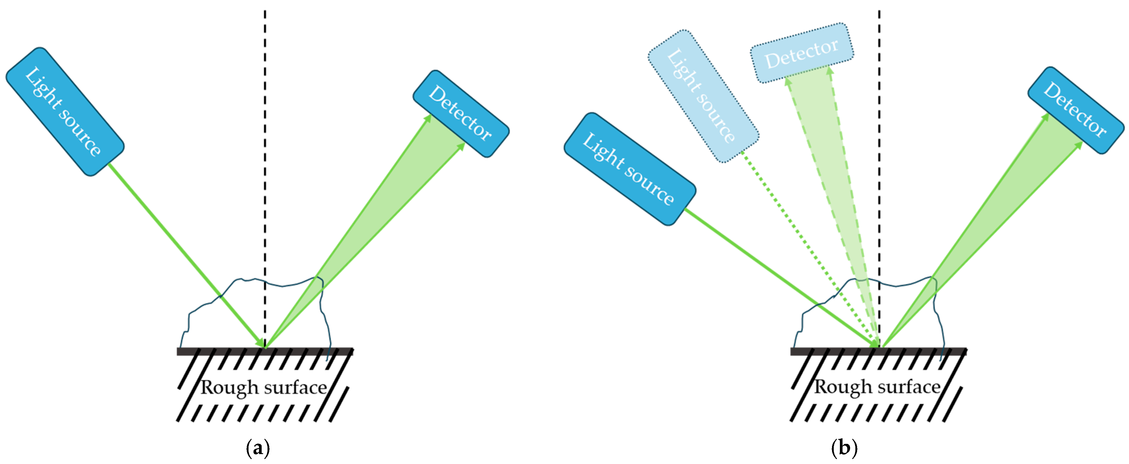
For evaluating surface roughness with reduced BRDF data, several groups have proposed to use the configuration shown in Figure 2a [19,20], where only a part of the BRDF with a fixed incident angle is measured. For the cases where the characteristic mapping between the measured range of BRDF data and the surface roughness is prominent and without ambiguity, the configuration is quite compact and efficient. However, the surface topology of a rough surface is eventually random, and therefore the repeatability and the sensitivity to the fluctuation of measurement conditions can be an issue. For acquiring more data with significantly different characteristic mapping, i.e., different incident angle and range of BRDF data, for double checking to ensure the reliability of the evaluation, the configuration with multiple light sources and detectors shown in Figure 2b can be adopted as an extended version. However, the whole installation becomes bulkier.
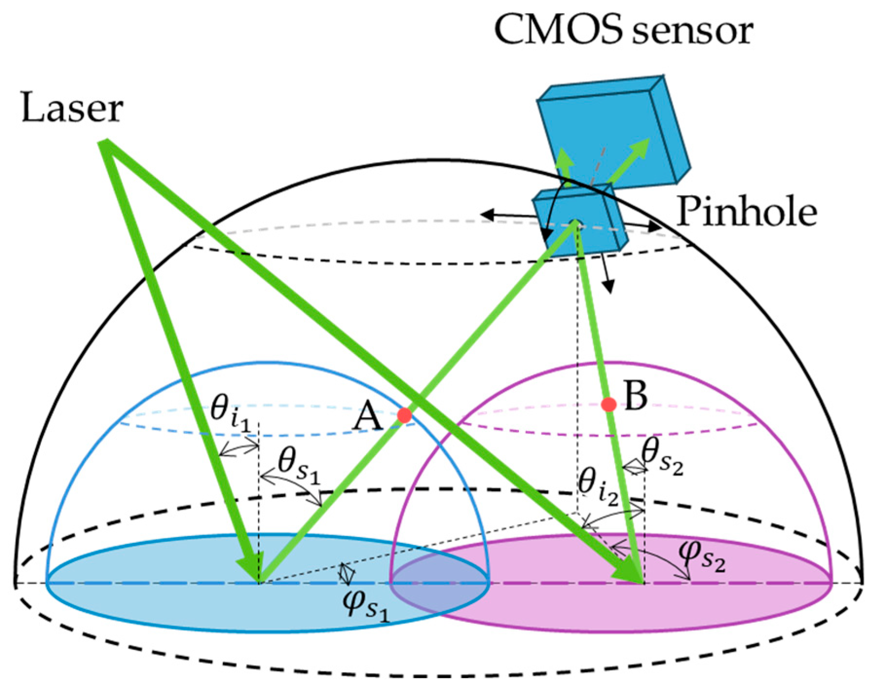
For resolving all the above-mentioned issues simultaneously, a configuration capable of measuring multiple sets of reduced BRDF with significantly different characteristic mapping relationships with surface roughness by exploiting a single light source and a single detector is proposed, as shown in Figure 3. In this case, two points of BRDF data are taken as an example. A laser beam is split into two by a grating and incident on two points of the target surface. The angular intensity of a part of the scattering pattern from these two surface points is simultaneously detected by an area detector (e.g., a complementary metal–oxide–semiconductor (CMOS) sensor) with a pinhole in front. From the light path shown in Figure 3, the scattering angle to be chosen for the angular intensity detection is determined by the geometry of the overall layout, including laser, grating, pinhole, and CMOS sensor. The data process module shown in Figure 3 is implemented on an external computer. Therefore, it is necessary to make big data analysis on the scattering pattern of the target surface with different incident angles to search for the useful BRDF datasets having unambiguous characteristic mapping with surface roughness. The geometrical layout of the whole configuration needs to accommodate for acquiring those BRDF data. In addition, for this configuration to be valid for surface roughness evaluation, the surface property must be uniform over the area of the target surface to be detected.

3. BRDF Measurement and Database Analysis

In this study, the standard specimen of roughness made with electrical discharge machining from Sodick Co., Ltd. (Kiyosu, Aichi, Japan), was used as shown in Figure 4. The roughness cover Ra values range from 0.13 µm to 2.1 µm, with 10 roughness grades. Each test sample has a size of 12 × 12 mm.
Ra normally has a proportional relationship with RMS roughness σ as expressed in Equation (7), where β is a coefficient related to the surface property [27], and it is between 1.2 and 1.3 for the reference sample being used.
σ β · R a
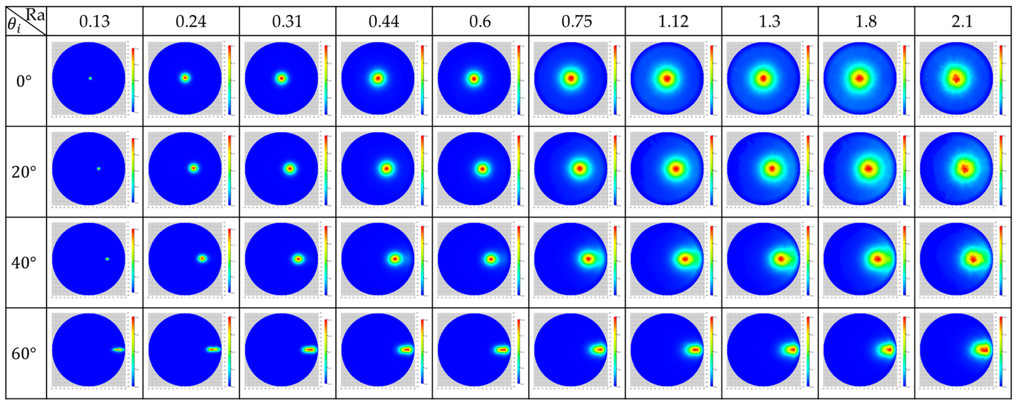
To make big data analysis for finding the useful part of reduced BRDF data to evaluate the surface roughness, the Mini-Diff VPro scatterometer from Synopsys, Inc. (Sunnyvale, CA, USA) is used for acquiring the BRDF of the reference sample. This commercial device provides RGB illumination channels—blue (465 nm), green (525 nm), and red (630 nm). Among them, the green channel (525 nm) is used for data acquisition because it lies near the spectral center and yields reliable signal intensity for the measurements. Accordingly, the chosen wavelength for measurement is 525 nm, and the incident angles to be taken are θ i = 0°, 20°, 40°, and 60°, where a 20° gap is considered large enough for finding datasets with significantly different characteristic mapping with surface roughness. Figure 5 shows the measurement result, which indicates that sufficient BRDF pattern variation has already been obtained to distinguish the surface roughness of the reference sample.
The proposed approach requests to draw certain reduced BRDF data for evaluating the surface roughness, and the most straightforward relationship is the angular intensity at a specific incident angle and scattering angle increases or decreases monotonically with the change in surface roughness. Therefore, this becomes the major target for big data analysis. The denotation used in the algorithm is illustrated in Figure 6.
The algorithm is written with Python (version 3.8.5), and the procedure is as follows:
1.
Build up BRDF database by sorting out the data with surface roughness Ra, incident angle ( θ i , φ i ) and observation angle ( θ s , φ s ) . The database can be expressed as
D a t a b a s e = B R D F R a ,   θ i , φ i , θ s , φ s
2.
Funding the combination of incident angle ( θ i , φ i ) and observation angle ( θ s , φ s ) , for which BRDF value changes monotonically with surface roughness. The algorithm is expressed as
B R D F + c o r r .   R a n ,   θ i , φ i , θ s , φ s < B R D F + c o r r .   R a n + 1 ,   θ i , φ i , θ s , φ s
and
B R D F c o r r .   R a n ,   θ i , φ i , θ s , φ s > B R D F c o r r .   R a n + 1 ,   θ i , φ i , θ s , φ s
where R a n 0.13 , 2.1 μ m   θ i = 20 ° , 40 ° , 60 ° ; φ i = 0 ° ; θ s [ 0 ° , 90 ° ] ; φ s 0 ° , 360 ° .
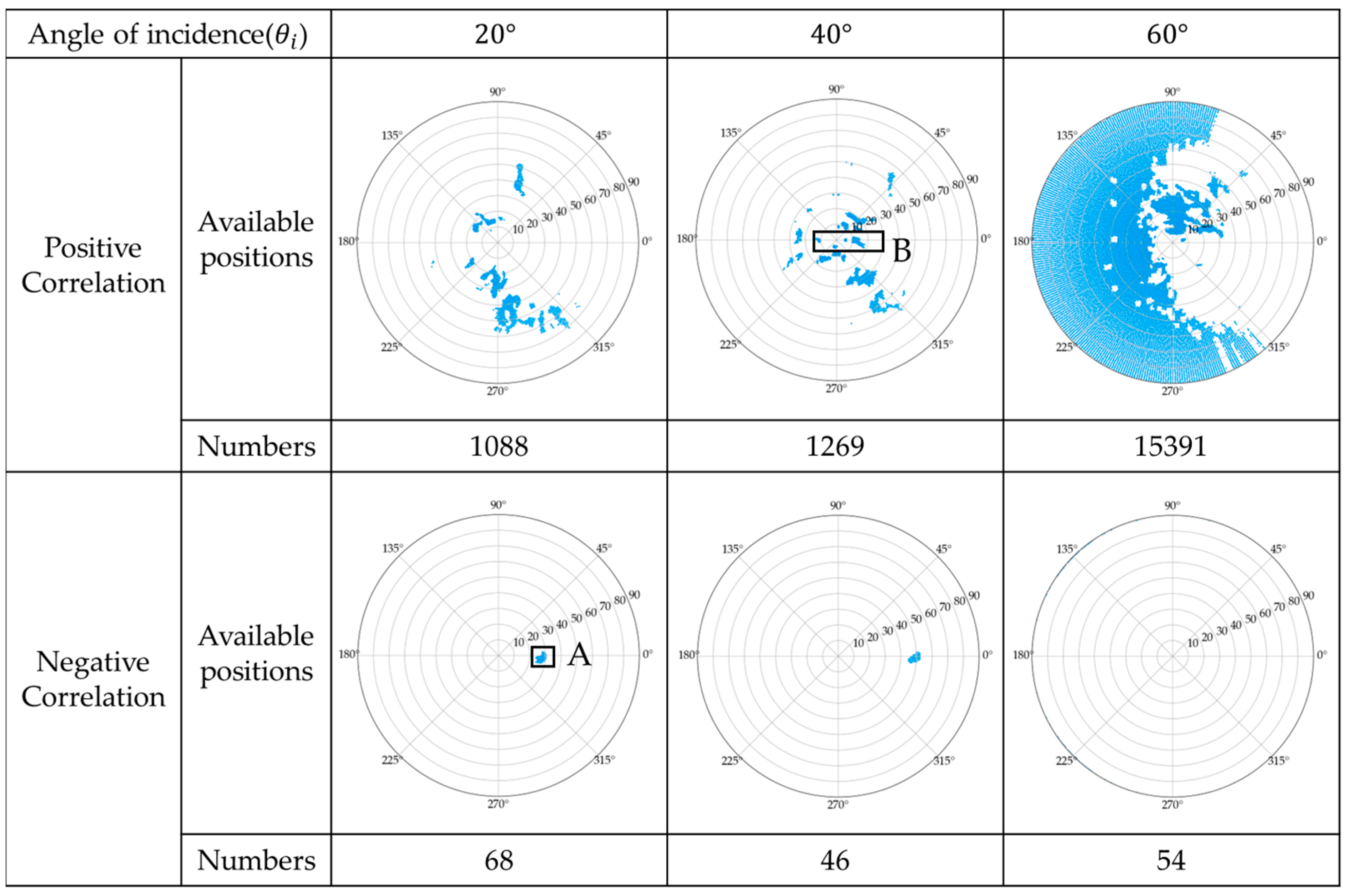
θ i = 0° has been ruled out in the searching due to potential mechanical interference between the light source and the sensor in practice, even if the dataset is useful, as can be seen from Figure 6. The final result is shown in Figure 7, where blue dots mark the scattering angles where the BRDF value increases or decreases monotonically with the increase in surface roughness.
It is clear that the scattering angles with negative correlations are much fewer than those with positive correlation. Therefore, the one with negative correlation should be selected first. Within the area marked with A at the incident angle of 20°, there are 68 scattering angles nearby to each other with similar characteristics. This also implies high stability of this negative correlation around that angular range. The one to be selected is θ i 1 , φ i 1 , θ s 1 , φ s 1 = ( 20 ° , 0 ° , 30 ° , 0 ° ) . Once these data are chosen, the selection of the other data with positive correlation would have some constraints due to the limited area of the sensor, as can be seen from Figure 6, even with some tunable parameters, such as the pinhole distance from the test sample. The area marked with B at the incident angle of 40° roughly shows the area covering the available choice. If a similar estimation is conducted for 60°, not only the constrained area becomes tighter and covers no available data, but also the required area of test target becomes much larger. Within area B shown in Figure 7, there are quite a few scattering angles aggregating together around θ s 2 , φ s 2 = ( 14 ° , 0 ° ) , which also implies the high stability of the positive correlation around that angle. Therefore, the second dataset to be selected is   θ i 2 , φ i 2 , θ s 2 , φ s 2 = ( 40 ° , 0 ° , 14 ° , 0 ° ) .
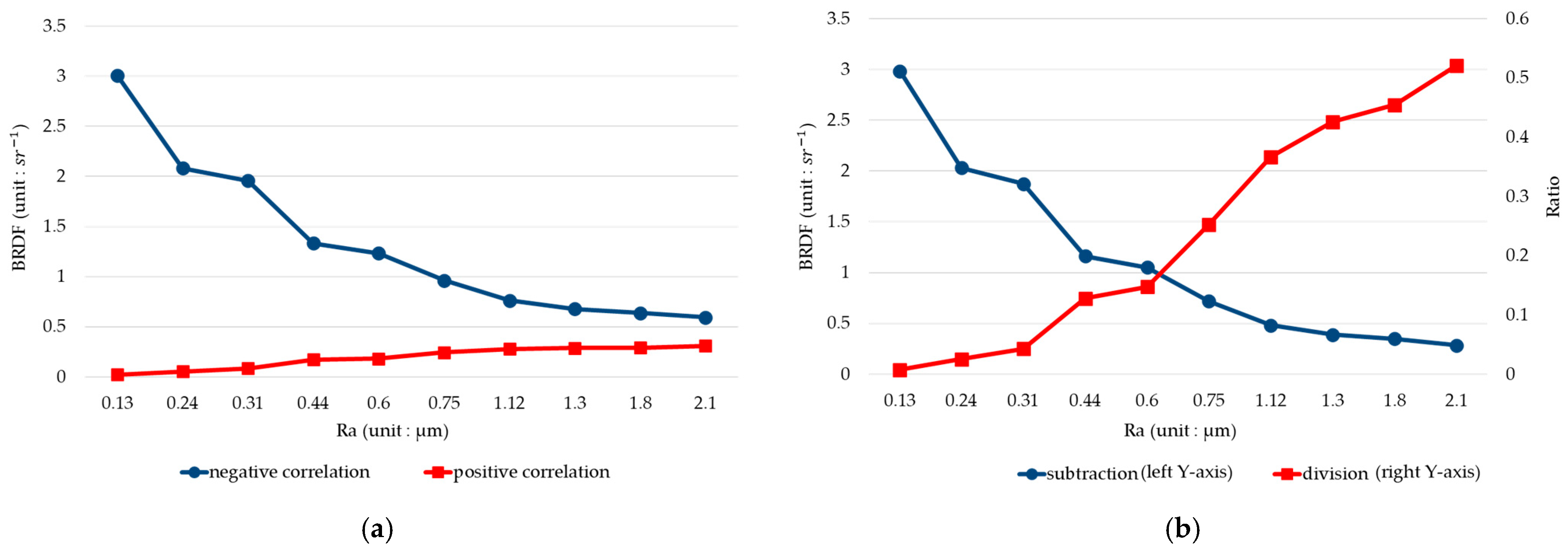
The relationship between the BRDF dataset and the surface roughness is quantitatively plotted in Figure 8a for both the selected positive and negative correlation ones. It indicates that the one with positive correlation has a shallow slope, which implies less immunity to the fluctuation in the measurement, hence less reliability. As the two datasets have opposite correlations with surface roughness, the division or subtraction of these two datasets could lead to a larger slope or higher sensitivity of the correlation with surface roughness. The division and the subtraction of these two datasets are plotted in Figure 8b. Notably, dual Y-axes are utilized to separately represent BRDF values for subtraction (left axis) and unitless ratio for division (right axis), providing a clearer comparison of how the combined use of the two metrics enhances sensitivity to surface roughness. As all these relationships shown in Figure 8 are monotonic, they all can be used alone or together as a lookup table mapping for evaluating the surface roughness without ambiguity.

4. Prototype and Experiment

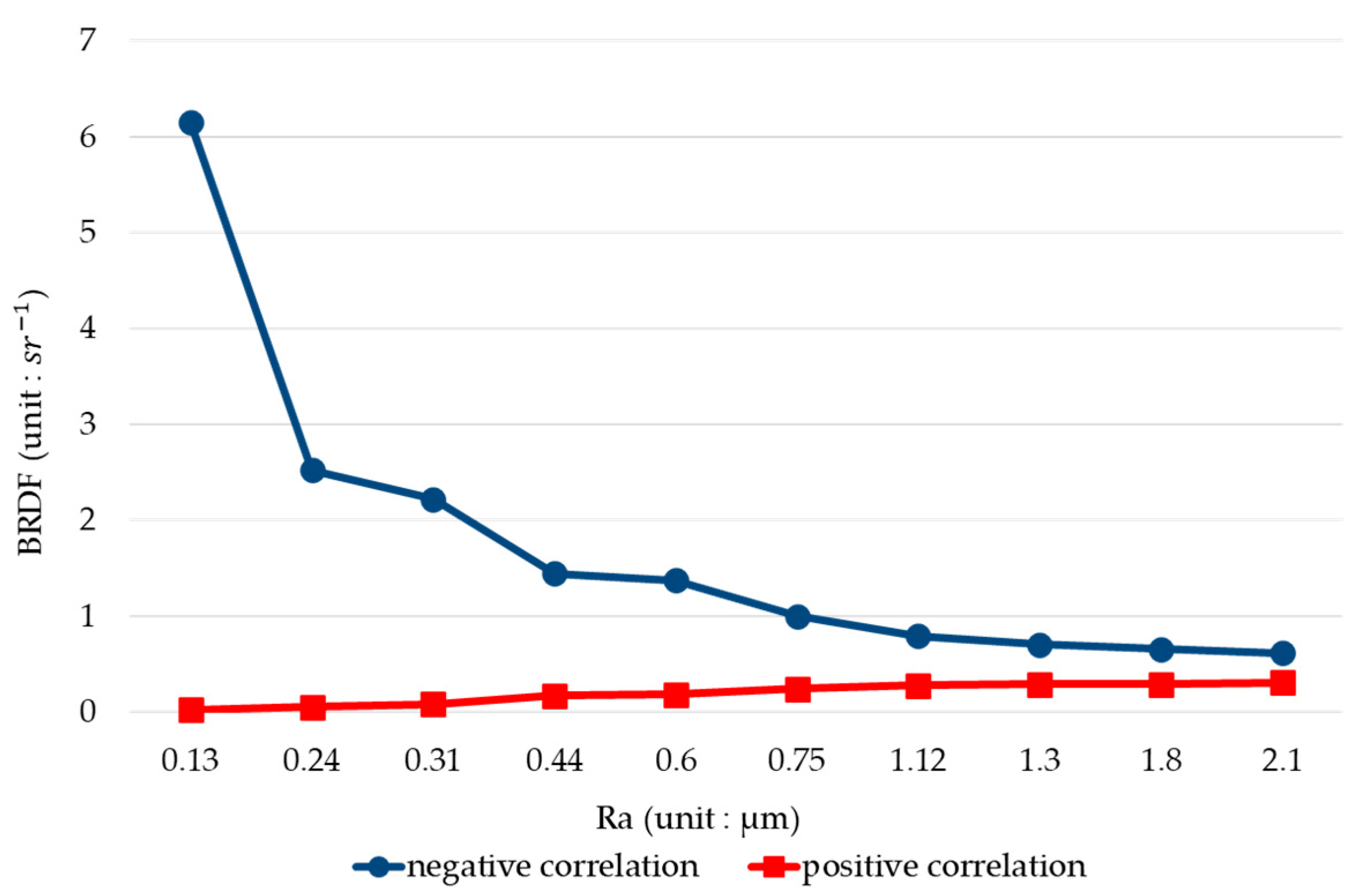
Based on the measurement and data analysis in Section 3, the proposed measurement configuration should be geometrically laid out to accommodate the selected two BRDF datasets, θ i 1 , φ i 1 , θ s 1 , φ s 1 = 20 ° , 0 ° , 30 ° , 0 °   and   θ i 2 , φ i 2 , θ s 2 , φ s 2 = ( 40 ° , 0 ° , 14 ° , 0 ° ) . The geometrical denotation for the measurement setup is shown in Figure 9. The grating tile angle is α and the diffraction angle of ± 1 order is ± θ . Therefore, θ i 1 = α θ and θ i 2 = α + θ . The distance between two laser beam spots on the surface is d, which can be tuned with the distance between the grating and the surface. The grating in the experiment has a periodic structure of 300 lines/mm, and the laser has a wavelength of 520 nm. This value is selected to closely match the 525 nm channel of the reference device, minimizing spectral mismatch in comparative analysis. θ is evaluated to be 9°. The distance between the grating and the surface is tuned to h = 21 mm to make d = 9 mm. The pinhole size is 1 mm in diameter, which can be considered as a single point. Its tilt angle and the distance from the zeroth-order diffraction position on the sample surface are δ = 23° and r = 32 mm, respectively, enabling acquisition of the angular intensity at the closest scattering angle as desired. With all geometrical calculation fixed, the final dataset becomes θ i 1 , φ i 1 , θ s 1 , φ s 1 = ( 21 ° , 0 ° , 29 ° , 0 ° ) and   θ i 2 , φ i 2 , θ s 2 , φ s 2 = ( 39 ° , 0 ° , 14 ° , 0 ° ) , slightly different from what obtained in Section 3. The BRDF with the incident angle at 21° and 39° are measured with scatterometer and the result is shown in Figure 10. The corresponding relationship of the BRDF datasets with surface roughness is plotted in Figure 11, which shows the monotonic relationship is maintained.
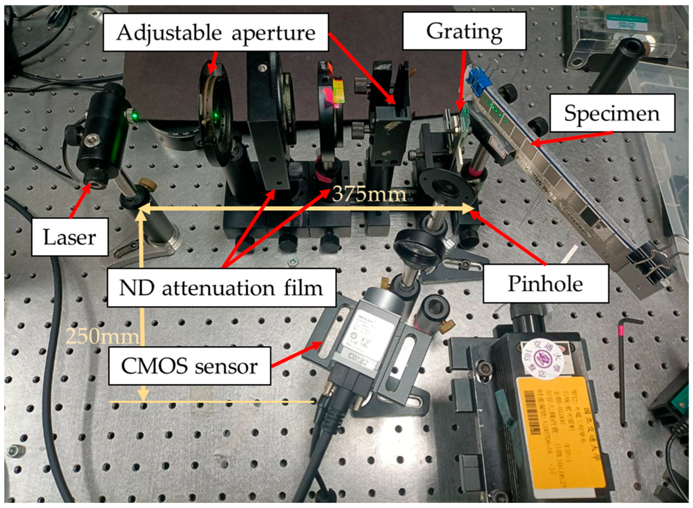
The experimental setup of the proposed configuration is shown in Figure 12. The overall footprint of the setup is approximately 375 mm × 250 mm × 150 mm. While the current prototype has not yet been optimized for miniaturization, the separated illumination and reception design allow future flexibility. By adjusting the geometric parameters h, d, and r, the spatial constraints of on-machine or in-line configurations can be addressed, offering a path toward practical deployment in restricted spaces such as near machine spindles. In the current setup, the laser beam is attenuated using a neutral density (ND) film and shaped by multiple adjustable apertures. As the sample size for each roughness is not sufficiently large, measurement of each roughness sample takes two steps. The first step moves the sample so as to make the laser beam incident at 21° right at the center of the sample, as shown in Figure 13a, and the corresponding valid spot on the CMOS sensor is shown underneath marked with a red circle, which represents the +1st diffraction order. The dashed circle marks the zeroth-order diffraction position. The second step then shifts the sample laterally so that the laser beam incident is at 39° right at the center of the sample, as shown in Figure 13b, and the corresponding valid spot on the CMOS sensor shown underneath is also marked with a yellow circle, which indicates the −1st diffraction order, while the dashed circle again represents the zeroth-order diffraction position. The procedure also ensures that the condition of uniform roughness property can be met. The measured spot distribution is integrated together as the ARS expressed in Equation (4), and the corresponding BRDF is then calculated with Equation (5).
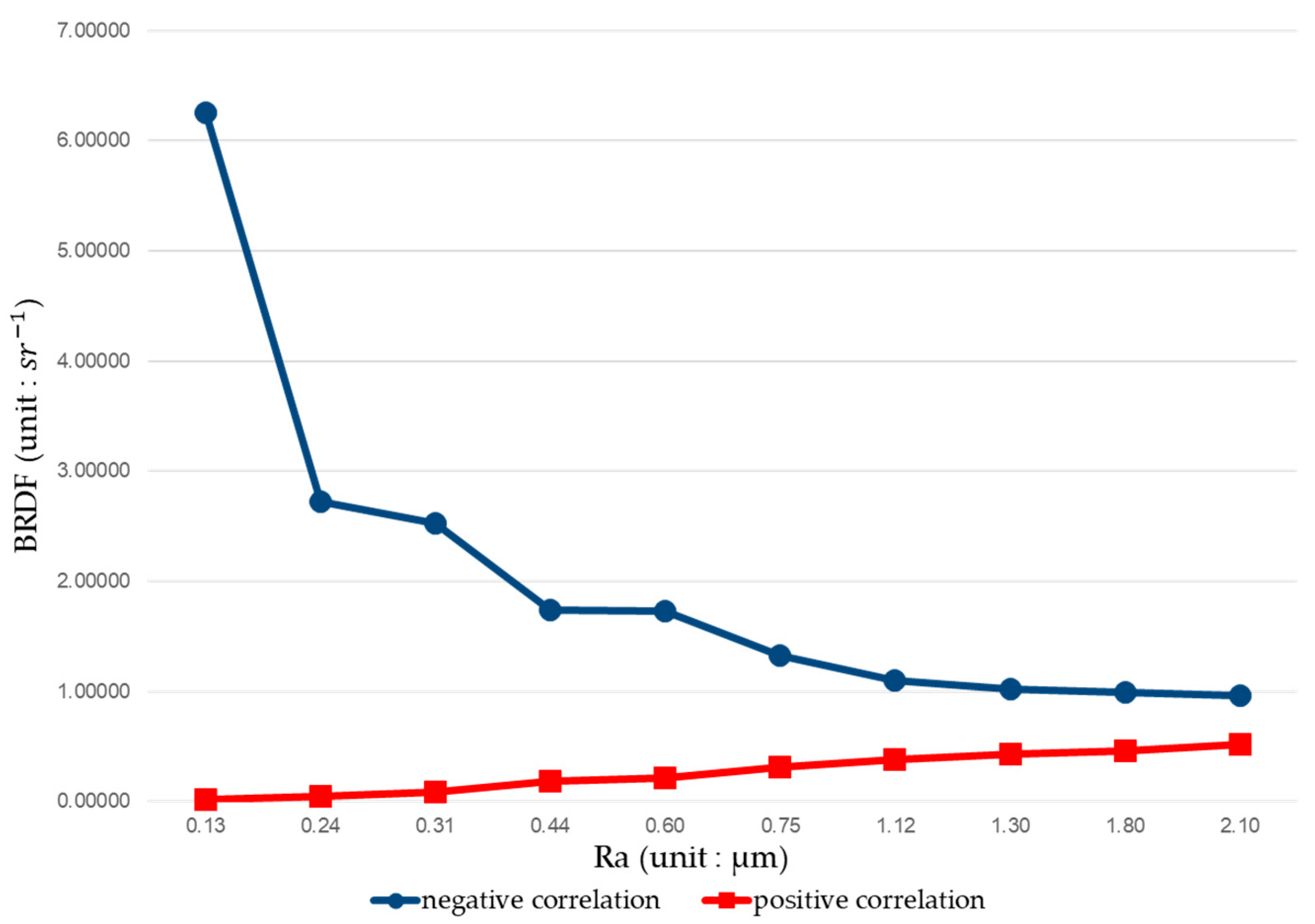
The BRDF value versus roughness for θ i 1 , φ i 1 , θ s 1 , φ s 1 = ( 21 ° , 0 ° , 29 ° , 0 ° ) and θ i 2 , φ i 2 , θ s 2 , φ s 2 = ( 39 ° , 0 ° , 14 ° , 0 ° ) from the experiment are plotted in Figure 14, with the one from scatterometer shown in Figure 11 as dot line for reference. There is a scaling factor in between due to the different sensitivity and calibration of the sensors being used, but the proportional coefficient remains almost constant, hence the trend of the relationship between the BRDF and the roughness. Note that the grayscale values obtained from the proposed system have been calibrated and converted to equivalent BRDF values (unit: sr−1) through the implemented algorithm, enabling a direct comparison with the commercial scatterometer data.
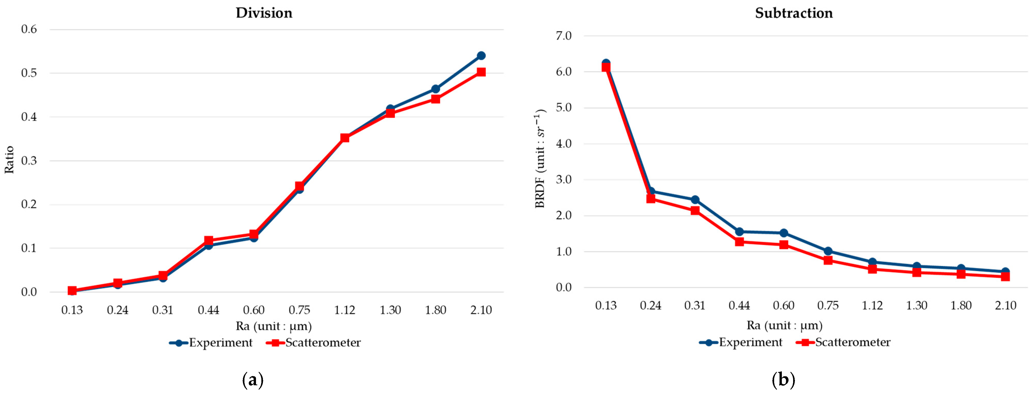
If making a division of two datasets from the experiment, the scaling factor should be canceled and the value becomes unitless. Figure 15a shows the comparison of the division value versus roughness from the proposed system (labeled as “experiment”) and scatterometer, which shows quite a good match, with slight deviation at the roughness values of 0.44 µm, 1.8 µm, and 2.1 µm. Figure 15b shows the subtraction of two BRDF datasets from the experiment versus roughness, which could be beneficial for canceling the common noise in measuring two datasets, such as white noise. Similarly, as all these relationships shown in Figure 14 and Figure 15 are monotonic, they all can be used alone or together as a lookup table mapping for evaluating the surface roughness without ambiguity.

5. Discussions

Optical scattering at a rough surface is inherently a random process, and therefore the approach of using reduced BRDF for roughness evaluation is not as generic as that shown in Equations (2)–(6). As a consequence, the evaluation is valid only for the condition to be investigated. Taking the case in this study as an example, if the rough surface is not made with electric discharge machining, the relationship between the reduced BRDF and the roughness might be different even for the same roughness value and range. In addition, evaluating the roughness with interpolation of the data can also be highly susceptible, because the slope in the relationship between the BRDF and the roughness varies significantly without showing any regular rule. Nevertheless, a bigger database associated with deep learning process could improve the robustness and reliability of the evaluation and extend the applicability of the concept [28,29,30]. The proposed configuration provides an opportunity at hardware level which allows collection of more data with significantly different characteristics mapping relationships simultaneously.
Although these limitations exist, the method’s compact hardware configuration and data-efficient algorithm still offer practical benefits for in-line surface screening in constrained environments. In the proposed configuration, the pinhole is used to select the scattering angle to be detected for the angular intensity. However, if the pinhole size is increased, the configuration becomes a compact version of the one shown in Figure 2b. Certainly, the pinhole cannot be as large as that two reduced BRDF patterns overlap on the sensor. The reason for compactness is that only one light source and one area sensor are used, with the need of larger size test surface and uniform surface property over the test area. In addition, the degree of freedom for choosing the combination of incident angle and scattering angle becomes limited.
For realizing the proposed configuration, there have been quite a few components available to support the hardware establishment. A kind of diffractive optical element referred to as Dammann grating [31,32,33] can split a laser source into several beams in two dimensions with high uniformity, and the diffraction angle can be designed to accommodate to what is required in the installation.
Although the current implementation is not yet fully optimized for footprint, future modularization based on optical component selection and separation of optical paths (illumination vs. detection) provides flexibility to adapt the configuration for different industrial integration scenarios.

6. Conclusions

This study validates a novel approach for simplified BRDF-based surface roughness evaluation, demonstrating promising application potential in real-time and in-line industrial settings.
  • Proposes a compact system using a single light source and a single CMOS sensor for BRDF-based roughness detection;
  • Requires only two angular intensities, enabling high-speed acquisition (<100 ms) with low processing overhead;
  • The configuration offers potential for in-line integration using beam-splitting optical elements such as Dammann gratings, which generate uniform multi-beam patterns with customizable diffraction angles;
  • Validates the method on EDM-processed specimens with Ra from 0.13 µm to 2.1 µm, showing strong correlation with commercial BRDF results;
  • Acknowledges limitations such as material dependency, angular sensitivity, and limited Ra range;
  • Plans future work to address broader material compatibility, uncertainty analysis, and model retraining for extended roughness ranges.

Author Contributions

Conceptualization, J.-H.Y. and C.-H.C.; methodology, J.-H.Y.; validation, J.-H.Y. and Z.-Y.F.; formal analysis, J.-H.Y.; investigation, Z.-Y.F.; resources, C.-H.C.; data curation, Z.-Y.F.; writing—original draft preparation, J.-H.Y.; writing—review and editing, C.-H.C.; visualization, Z.-Y.F.; supervision, C.-H.C.; project administration, C.-H.C.; funding acquisition, C.-H.C. All authors have read and agreed to the published version of the manuscript.

Funding

This research was funded by the National Science and Technology Council (NSTC), Taiwan, under grant number MOST 109-2221-E-009-158.

Institutional Review Board Statement

Not applicable.

Informed Consent Statement

Not applicable.

Data Availability Statement

The original contributions presented in this study are included in the article. Further inquiries can be directed to the corresponding author.

Acknowledgments

The authors would like to thank IGIANT Optics Co., Ltd. for providing the roughness specimens and for assisting with the verification of the surface roughness measurements.

Conflicts of Interest

The authors declare no conflict of interest.

References

  1. Han, W.; Kim, W.-C.; Park, N.-C. A Novel Approach to Surface Roughness Quantification in Semiconductor Packaging Using Quantitative Metrics Based on BRDF Analysis. Opt. Laser Technol. 2025, 185, 112578. [Google Scholar] [CrossRef]
  2. Peterson, G.L. A BRDF model for scratches and digs. In Proc. SPIE 8495, Reflection, Scattering, and Diffraction from Surfaces III; 84950G, 15 October 2012; SPIE: Bellingham, WA, USA, 2012. [Google Scholar] [CrossRef]
  3. ISO 4288: 1996; Geometrical Product Specifications (GPS)—Surface Texture: Profile Method—Rules and Procedures for the Assessment of Surface Texture. Edition DIN EN ISO 4288. European Committee for Standardization: Brussels, Belgium, April 1998.
  4. ISO 4287:1997; Geometrical Product Specifications (GPS)—Surface Texture: Profile Method—Terms, Definitions and Surface Texture Parameters, 1st ed. International Organization for Standardization: Geneve, Switzerland, 1 April 1997.
  5. ISO 25178-600:2019; Geometrical Product Specification (GPS)—Surface Texture: Areal—Metrological Characteristics for Areal Topography Measuring Methods. ISO: Geneva, Switzerland, 2019. Available online: https://www.iso.org/standard/67651.html (accessed on 20 February 2025).
  6. Whitehouse, D.J. Handbook of Surface Metrology; IOP Publishing Ltd.: Bristol, UK, 1994. [Google Scholar]
  7. Degarmo, E.P.; Black, J.T.; Kohser, R.A. Materials and Processes in Manufacturing, 9th ed.; Wiley: Hoboken, NJ, USA, 2003; ISBN 0-471-65653-4. [Google Scholar]
  8. Williams, H. Influence of Curved Surface Roughness on White Light Interferometer Microscopy. Phys. Educ. 2022, 57, 015001. [Google Scholar] [CrossRef]
  9. Hariharan, P. Basics of Interferometry, 2nd ed.; Academic Press: New York, NY, USA, 2007. [Google Scholar]
  10. Wyant, J.C. White Light Interferometry. Proc. SPIE 2002, 4737, 103. [Google Scholar] [CrossRef]
  11. Udupa, G.; Singaperumal, M.; Sirohi, R.S.; Kothiyal, M.P. Characterization of Surface Topography by Confocal Microscopy: I. Principles and the Measurement System. Meas. Sci. Technol. 2000, 11, 305–314. [Google Scholar] [CrossRef]
  12. Mauch, F.; Osten, W. Model-Based Approach for Planning and Evaluation of Confocal Measurements of Rough Surfaces. Meas. Sci. Technol. 2014, 25, 105002. [Google Scholar] [CrossRef]
  13. Jordan, H.-J.; Wegner, M.; Tiziani, H. Highly Accurate Non-Contact Characterization of Engineering Surfaces Using Confocal Microscopy. Meas. Sci. Technol. 1999, 9, 1142–1151. [Google Scholar] [CrossRef]
  14. Stover, J.C. Optical Scattering Measurement and Analysis; SPIE Press: Bellingham, WA, USA, 2012. [Google Scholar]
  15. Bihan, Q.K.-L. From BRDF to Roughness: Defining the Link between Two Key Parameters for Optical Design. In Optical Systems Design 2015: Illumination Optics IV; SPIE: Bellingham, WA, USA, 2015; Volume 9629. [Google Scholar] [CrossRef]
  16. Ali, A.; Nishino, K.; Ikeuchi, K. Efficient Modeling of Objects BRDF with Planned Sampling. IPSJ Trans. Comput. Vis. Appl. 2013, 5, 114–118. [Google Scholar] [CrossRef]
  17. Prabhakar, D.V.N.; Gopala Krishna, A.; Sreenivasa Kumar, M. Analysis on Significance of Various Statistical Texture Features in Vision-Based Surface Roughness Prediction in End Milling Process. Int. J. Interact. Des. Manuf. 2023, 17, 1563–1577. [Google Scholar] [CrossRef]
  18. Persson, U. In-Process Measurement of Surface Roughness Using Light Scattering. Wear 1998, 215, 54–58. [Google Scholar] [CrossRef]
  19. Feidenhans’l, N.A.; Hansen, P.-E.; Pilný, L.; Madsen, M.H.; Bissacco, G.; Petersen, J.C.; Taboryski, R. Comparison of Optical Methods for Surface Roughness Characterization. Meas. Sci. Technol. 2015, 26, 085208. [Google Scholar] [CrossRef]
  20. Lu, R.-S.; Tian, G.Y. On-Line Measurement of Surface Roughness by Laser Light Scattering. Meas. Sci. Technol. 2006, 17, 1496–1502. [Google Scholar] [CrossRef]
  21. Masaki, T.; Kawata, K.; Masuzawa, T. Micro Electro-Dsicharge Machining and Its Applications; IEEE: New York, NY, USA, 1990. [Google Scholar]
  22. Nicodemus, F.E. Directional reflectance and emissivity of an opaque surface. Appl. Opt. 1965, 4, 767–775. [Google Scholar] [CrossRef]
  23. Luan, C.; Li, Y.; Guo, H.; Sun, H.; Zhang, L.; Zheng, H.; Zhang, X. Modified Model of Polarized Bidirectional Reflectance Distribution Function Used for Light Detection and Ranging (LiDAR). Photonics 2023, 10, 1119. [Google Scholar] [CrossRef]
  24. Schröder, S.; Duparré, A.; Coriand, L.; Tünnermann, A.; Penalver, D.H.; Harvey, J.E. Modeling of light scattering in different regimes of surface roughness. Opt. Exp. 2011, 19, 9820–9835. [Google Scholar] [CrossRef] [PubMed]
  25. Georgiev, G.T.; Speck, D.R.; Johnson, D.D. Scatter Light Measurements in Support of Optical Instruments Development. In Proceedings of the 24th Annual Mirror Technology SBIR/STTR Workshop, Greenbelt, MD, USA, 18–21 November 2024; NASA: Washington, DC, USA, 2024. [Google Scholar]
  26. Younis, M.A. On Line Surface Roughness Measurements Using Image Processing towards an Adaptive Control. Computers 1998, 35, 49–52. [Google Scholar] [CrossRef]
  27. Aulbach, L.; Salazar Bloise, F.; Lu, M.; Koch, A.W. Non-Contact Surface Roughness Measurement by Implementation of a Spatial Light Modulator. Sensors 2017, 17, 596. [Google Scholar] [CrossRef] [PubMed]
  28. Shang, S.; Wang, C.; Liang, X.; Cheung, C.F.; Zheng, P. Surface Roughness Prediction in Ultra-Precision Milling: An Extreme Learning Machine Method with Data Fusion. Micromachines 2023, 14, 2016. [Google Scholar] [CrossRef] [PubMed]
  29. Wu, D.; Wei, Y.; Terpenny, J. Surface roughness prediction in additive manufacturing using machine learning. In Proceedings of the International Manufacturing Science and Engineering Conference, American Society of Mechanical Engineers, College Station, TX, USA, 18–22 June 2018; Volume 51371, p. V003T02A018. [Google Scholar]
  30. Guo, M.; Wei, S.; Han, C.; Xia, W.; Luo, C.; Lin, Z. Prediction of Surface Roughness Using Deep Learning and Data Augmentation. J. Intell. Manuf. Spec. Equip. 2024, 5, 221–241. [Google Scholar] [CrossRef]
  31. Krackhardt, U.; Streibl, N. Design of Dammann-Gratings for Array Generation. Opt. Commun. 1989, 74, 31–36. [Google Scholar] [CrossRef]
  32. Jahns, J.; Downs, M.M.; Prise, M.E.; Streibl, N.; Walker, S.J. Dammann Gratings for Laser Beam Shaping. Opt. Eng. 1989, 28, 281267. [Google Scholar] [CrossRef]
  33. Jia, J.; Zhou, C.; Liu, L. Circular Dammann Grating and Its Applications. In Nano-Optics and Nano-Structures; Zhu, X., Chou, S.Y., Arakawa, Y., Eds.; International Society for Optics and Photonics (SPIE): Bellingham, WA, USA, 2002; Volume 4923, pp. 119–126. [Google Scholar] [CrossRef]
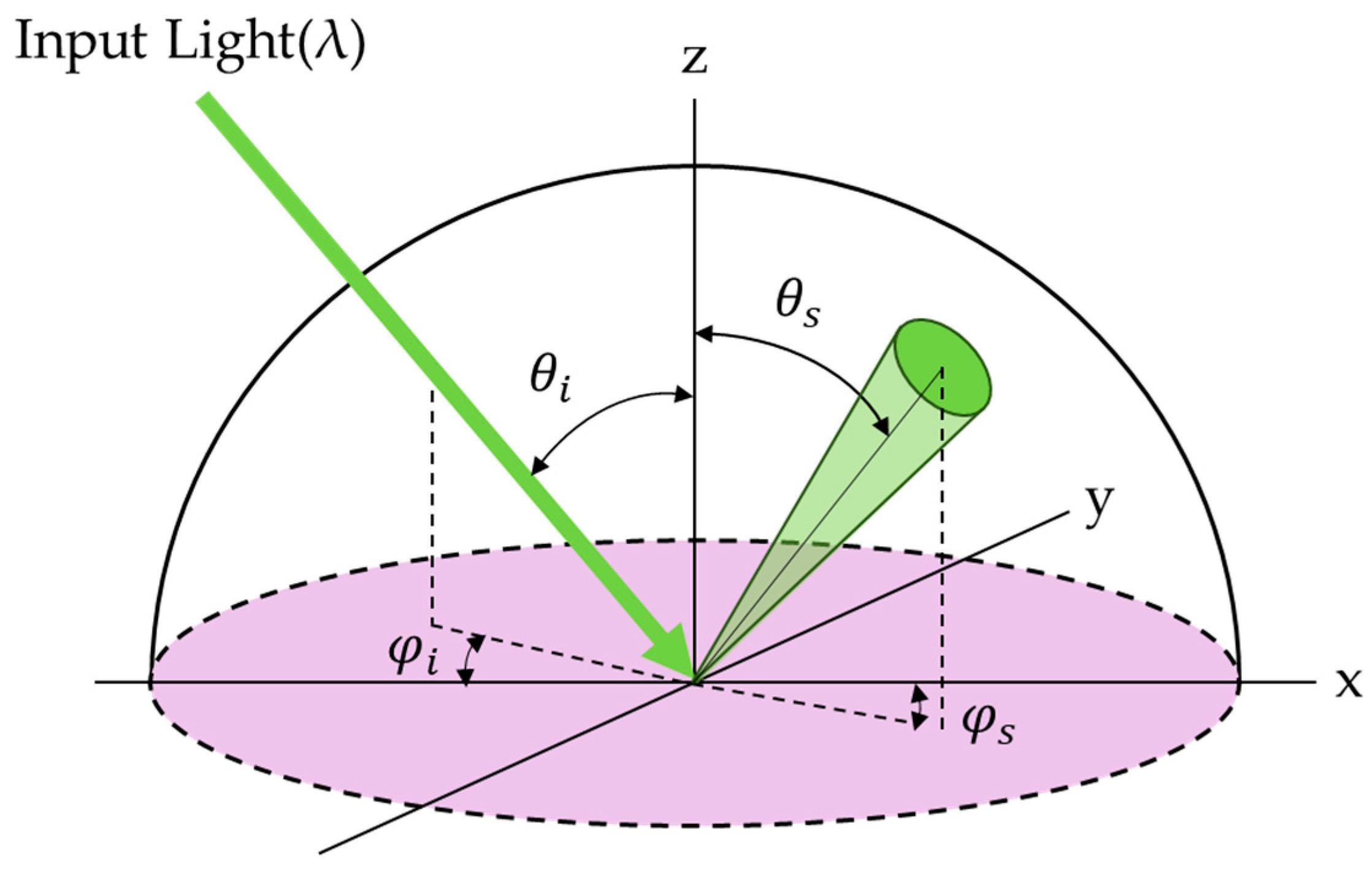
Figure 1. Schematic diagram of scattering measurement.
Applsci 15 09850 g001
Figure 2. Configurations for measuring reduced BRDF data: (a) single light source and detector; (b) multiple light sources and detectors.
Applsci 15 09850 g002
Figure 3. Configuration for measuring multiple sets of reduced BRDF with a single light source and a detector.
Applsci 15 09850 g003
Figure 4. Standard specimen of roughness from Sodick. The ten samples, from left to right, correspond to Ra values of 0.13, 0.24, 0.31, 0.44, 0.6, 0.75, 1.12, 1.3, 1.8, and 2.1 µm.
Applsci 15 09850 g004
Figure 5. BRDF patterns of different surface roughness with incident angles at 0°, 20°, 40°, and 60°.
Applsci 15 09850 g005
Figure 6. Denotation for the reduced BRDF data. The two regions labeled A and B indicate candidate angular areas where the BRDF values increase or decrease monotonically with surface roughness.
Applsci 15 09850 g006
Figure 7. Scattering angles where BRDF value changes monotonically with surface roughness at incident angles of θ i = 20°, 40°, and 60°. The regions labeled A and B represent candidate angular areas with negative and positive correlations, respectively, used for selecting BRDF datasets in the analysis.
Applsci 15 09850 g007
Figure 8. Quantitative relationship between (a) BRDF datasets and surface roughness; (b) the division and subtraction of two BRDF datasets and surface roughness.
Applsci 15 09850 g008
Figure 9. Geometrical denotation for the reduced BRDF measurement setup.
Applsci 15 09850 g009
Figure 10. BRDF patterns of different surface roughness with incident angles at 21° and 39°.
Applsci 15 09850 g010
Figure 11. Quantitative relationship between BRDF datasets and surface roughness.
Applsci 15 09850 g011
Figure 12. Photograph of the experimental setup for the reduced BRDF measurement system, showing the laser, grating, specimen, pinhole, and CMOS sensor. Red arrows indicate the main optical components, and yellow lines denote the approximate physical dimensions of the system footprint.
Applsci 15 09850 g012
Figure 13. Angular intensity measurement on the CMOS sensor: (a) measurement with an incident angle of 21°, where the red circle indicates the +1st diffraction order, and the dashed circle marks the zeroth-order diffraction position; (b) measurement with an incident angle of 39°, where the yellow circle indicates the −1st diffraction order, and the dashed circle again marks the zeroth-order position.
Applsci 15 09850 g013
Figure 14. BRDF versus roughness from experimental data at θ i 1 , φ i 1 , θ s 1 , φ s 1 = ( 21 ° , 0 ° , 29 ° , 0 ° ) and θ i 2 , φ i 2 , θ s 2 , φ s 2 = ( 39 ° , 0 ° , 14 ° , 0 ° ) , which correspond to the negative and positive correlation datasets, respectively.
Applsci 15 09850 g014
Figure 15. Comparison of surface roughness measurements between the proposed system and the scatterometer: (a) result based on BRDF dataset division; (b) result based on BRDF dataset subtraction.
Applsci 15 09850 g015
Disclaimer/Publisher’s Note: The statements, opinions and data contained in all publications are solely those of the individual author(s) and contributor(s) and not of MDPI and/or the editor(s). MDPI and/or the editor(s) disclaim responsibility for any injury to people or property resulting from any ideas, methods, instructions or products referred to in the content.