Abstract
Methane emissions from freshwater reservoirs represent a globally relevant greenhouse gas source, which are estimated to range from 3% to 10% of all global anthropogenic methane emissions. However, there is high uncertainty in estimating reservoir emissions on local to global scales due to a combination of data paucity in key regions, particularly in the Southern Hemisphere, and challenges monitoring emission pathways. The key to improved spatially and temporally representative estimation of emission rates is to better understand the primary drivers of emission pathways, in particular, ebullition. We examine ebullition from 15 freshwater storages located in the Southern Hemisphere subtropical (South East Queensland) and temperate (Tasmania) regions using a combination of optical methane detection to develop the high-resolution mapping of ebullition zones and floating chamber incubation within ebullition zones to quantify areal emission rates. We demonstrate the equivalent water level, through air pressure or physical water level change, as a key driver of ebullition and examine the implications for spatially and temporally representative estimation of reservoir emissions. This study represents the largest broadscale ebullition survey undertaken across Australian temperate and subtropical reservoirs. The study findings are of broad relevance to scientists and corporate and government entities navigating the complexities of estimating greenhouse gas emissions from reservoirs and related policy instruments.
Keywords:
ebullition; subtropical; temperate; reservoirs; air pressure; water level; methane emissions 1. Introduction
Methane is a powerful greenhouse gas with a global warming potential of 28 times over a hundred-year timeframe [1]. It is critical to identify and quantify anthropogenic sources of methane to develop effective mitigation strategies to minimise its emissions. Reservoirs represent a small but important source of anthropogenic methane, i.e., an estimated 3–10% of all global anthropogenic methane emissions [2].
There is inherent variability in emissions from reservoirs, primarily due to the multiple emission pathways (diffusion, downstream, and ebullition), as well as multiple drivers of each pathway and temporal and spatial variability within the reservoir dynamics. Water temperature and eutrophication status have repeatedly been shown to influence emissions via all three pathways [3,4,5]; however, there are additional drivers of emissions for individual pathways. Additional drivers of diffusive emissions include surface water methane concentration, wind speed, and water current speed [6], with the resuspension of methane-enriched porewaters from littoral sediment zones [7] and oxic methanogenesis [8] modifying surface water concentrations. Additional drivers of downstream emissions include water intake depth, reservoir stratification status, dam structure release mechanism, and downstream flow regime [5,9].
Ebullition is increasingly recognised as the dominant emission pathway [10,11,12], but quantifying the rate of methane ebullition in water bodies is a uniquely difficult challenge as it can vary spatially over four orders of magnitude within 10 m [13]. Sediment bubble release is driven by many different factors including water level, sediment organic content, atmospheric pressure change, water depth, and surface wave action [14,15,16], which can undergo rapid variation over short temporal scales. In addition, emission rates in ebullition zones are two to four orders of magnitude higher than diffusive emissions; thus, ebullition in a relatively small surface area of a reservoir can contribute to the bulk of total emissions. For example, it was shown that less than 5% of Little Nerang Dam’s surface area contributes to over 95% of total methane emissions [13].
The development of global emission factors based on climate zones aims to reduce this inherent variability particularly for large, flooded land portfolios that cover several climate zones [1]. A further refinement in estimating emissions from large, flooded land portfolios is to scale emissions to water body eutrophication status using globally derived scaling factors [1]. However, estimation methods remain coarse and do not consider the spatial and temporal heterogeneity in processes driving emission releases across reservoirs globally. Nonetheless, the estimation of ebullition rates remains crucial for quantifying total reservoir emissions. The scientific understanding of the processes driving ebullition continues to improve; however, identifying the zones of ebullition within a reservoir and the reasonable estimation of ebullition remain challenging. This study aimed to determine if dropping equivalent water level increased ebullition activity in Australian subtropical and temperate water storages and to consider the implications of equivalent water level on the spatial and temporal representativeness of emission estimation.
2. Materials and Methods
2.1. Site Description
To address the study aim, ebullition patterns and emission rates were examined from 15 water storages located in the Southern Hemisphere subtropical (Southeast Queensland) and temperate (Tasmania) regions (Table 1; Figures S1 and S2). Storages in the subtropical region included 11 reservoirs and two weir systems across four reservoir size classes (Table 1). Water surface area of individual systems ranged from 0.2 to 109 km2 with a total flooded land surface area of 200 km2. In the temperate region, emissions from two large reservoirs were examined covering a total water surface area of 517 km2 (Table 1). Reservoir age ranged broadly with Enoggera Dam construction completed more than 150 years ago whilst Wyaralong Dam was only constructed 14 years ago (Table 1). The catchment area for individual storages ranged widely from 10 km2 for Gold Creek Dam to more than 10,000 km2 for Mt Crosby Weir (Table 1). Overall, this study examined emissions from more than 710 km2 of flooded land, which represents approximately 10% of Australia’s 7000 km2 of flooded land surface area [17]. To accommodate such a broad study, monitoring activities were undertaken across a series of field campaigns running over a 10-year period from 2013 to 2023. Noteworthily, site access is restricted to a number of these storages, and it was not possible to target the same month or season across all systems, and this represents a limitation of this study.

Table 1.
Water storage size, name, year of construction, water inundation area, catchment area, and climate for 13 reservoirs and 2 weirs. The size class was defined using the Global Reservoir and Dam (GRanD) classification [18].
2.2. Characterising Reservoir Ebullition Patterns
Ebullition zones were identified within each storage using optical methane detector (OMD) surveys to map ebullition activity and identify ebullition zones. Surveys followed the methodology detailed in [13], where the OMD was bow-mounted on the survey vessel and positioned to sweep the atmosphere immediately above the water surface (Figure 1A). Atmospheric methane concentrations were logged at 7 Hz, with ebullition detection defined by changes from the background concentration (Figure 1B) following [19]. Ebullition detections were separated from motor exhaust using relative wind speed and direction from an ultrasonic wind sensor (CruzPro UWSD10 3D Ultrasonic Wind Speed/Direction Sensor) mounted directly above the OMD logging at 2 Hz. These detections were only considered valid if the OMD was sweeping through new air across the water surface, and detections where the vessel was reversing or strong following winds were removed [19].
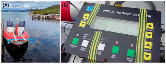
Figure 1.
(A) Open-path, optical methane detector (OMD), and ultrasonic wind sensor set up on survey vessel for ebullition transects. OMD swept atmospheric layer approximately 35 cm above water surface. Image taken on Lake Pedder, March 2022. (B) Two clear bubble detections during open-path, optical methane detector (OMD) ebullition transects showing elevated methane concentration relative to the background.
Ebullition detections were georeferenced using a logging GPS (1 Hz) mounted as close as practically possible to the OMD. Ebullition zones were defined using the criteria detailed in [13], where the zone is defined as multiple ebullition detections within 50 m of each other. Ebullition detections and water depth were georeferenced using a GPS depth sounder (Lowrance HDS7 depth sounder, Navico, Tulsa, OK, USA) logging at 1 Hz. To determine patterns and the depth relationships, georeferenced ebullition detections and water depth for all storages were visualised using the QGIS Geographic Information System (QGIS.org, 2025).
2.3. Equivalent Water Level as Ebullition Driver
The next step in this study was to quantify ebullition zone emission rates within each water storage during dropping and stable equivalent water level conditions. A single ebullition zone for each water storage was selected from the OMD surveys (Table S1) for subsequent floating chamber deployments to quantify the emission rates. The equivalent water level was estimated using the water level and air pressure changes during the chamber deployment [20]. Water storage levels were sourced from a national database [21] where levels are continuously updated at approximately hourly intervals. Air pressure data were sourced from the nearest available weather station accessed through the national mereological database [22] and converted to water level assuming that 1 hPa is approximately equal to a 1 cm water column [23]. Chamber deployments targeting dropping equivalent water levels exploited times of water withdrawal for drinking water supply, irrigation, or power generation, as well as the forecast passage of low-air pressure systems. Chamber deployments targeting stable equivalent water levels exploited times of no withdrawal for water supply, irrigation, or power generation, as well as the forecast passage of high-air pressure systems. Noteworthily, a similar limitation to the OMD surveys is relevant to this step as site access was restricted to a number of these storages and it was not possible to undertake chamber deployment in the same time period between field campaigns.
The floating chamber approach followed the methodology of [24] where the flux was calculated from the changes in chamber headspace concentration. A minimum of three chambers were deployed during each monitoring campaign, and individual chambers were placed in a tethered configuration at the same site for both dropping and stable equivalent water levels (Figure 2). This chamber deployment configuration ensures that chambers do not drift over the anchor weight where there is the potential for ebullition to occur due to weight movements in the sediments.
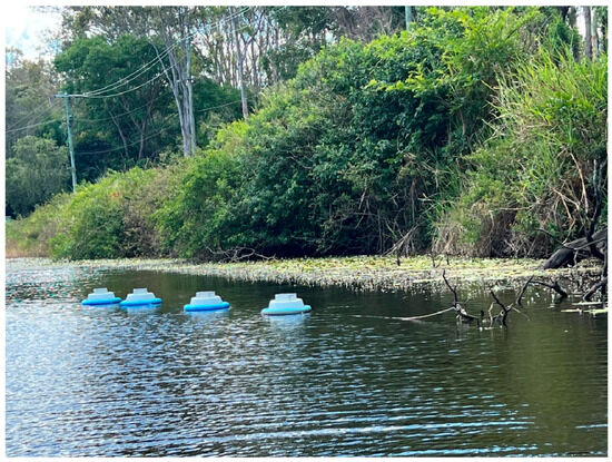
Figure 2.
Example of floating chamber deployment within reservoir ebullition zone. Image taken on Sideling Creek Dam, December 2022.
Chambers had the following characteristics: a diameter of 40 cm, 12 L headspace volume, and 0.7 kg weight; these chambers were placed on the water surface, and the headspace sample was manually collected prior to sealing the headspace and the time was recorded. At the completion of the deployment, the headspace sample was again collected manually and the time was recorded. The difference in headspace concentrations over the deployment period was then used to calculate the emission flux rates for individual replicate chambers [24].
In addition, the OMD surveys were undertaken to better understand the effect of water level and air pressure change on spatial ebullition activity in temperate reservoirs to compare against findings from previous studies on subtropical storages [13,24]. These surveys were undertaken on Lake Gordon and Lake Pedder following the methodology detailed in [24]. Survey timing on Lake Gordon was undertaken during a power production period with dropping water levels and during a period of no power production with stable water levels. The survey timing on Lake Pedder was undertaken during a period of stable water levels but exploited periods with rising or dropping ambient air pressure.
2.4. Data Analyses
Statistical analyses of ebullition water depth from the OMD surveys and chamber emission rates were undertaken using the Statistica (Version 13) software program [25]. Both the ebullition water depth and emission rate data failed to satisfy the assumptions of normality and homogeneity of variance even after transformation. Therefore, differences in ebullition water depth and emission rates were tested using the non-parametric Kruskal–Wallis (KW) test. Ebullition water depths from the OMD surveys were first classified as subtropical or temperate regions, and these regions were used as the categorical predictors. Emission rates from the chamber deployments were grouped according to equivalent water level status (dropping or stable), and these were used as the categorical predictors with chamber emission rates as the continuous variable. The reported statistical results were as follows: Kruskal–Wallis test values, the H statistic values, and the associated degrees of freedom with p-values.
To further explore regional ebullition water depth patterns, ebullition water depths from subtropical and temperate surveys were grouped into the following depth bins: less than 5 m deep; between 5 and 10 m deep; between 10 and 15 m deep; and greater than 15 m deep. Detections within each depth bin were summed and expressed as a percent of the total detections across each region. Depth bin selection follows the findings from Little Nerang Dam where major ebullition activity has shown to occur in the top 5 m with lower activity detected from 5 to 15 m depth and very rare detections below 15 m [13].
3. Results
3.1. Patterns of Ebullition
In total, over 1400 km of the optical methane detector surveys were undertaken during this study with ebullition detected across all subtropical and temperate systems surveyed. Ebullition zones were generally confined to the shallow water zones with fewer detections in deeper water surveys. In subtropical storages, the shallow water ebullition zones were primarily located in major catchment inflow arms with additional zones of activity within lateral inflows towards the dam wall (Figure 3; Supplementary Figures S3, S7–S9 and S11–S13). A notable exception to this pattern was Wyaralong Dam, where ebullition zones were primarily detected in deeper zones within the historic channel (Figure S14). The two oldest reservoirs, Enoggera Dam and Gold Creek Dam, had evidence of ebullition throughout the water body (Figures S5 and S6), as well as the two weirs, Mt Crosby Weir and O’Reilly’s Weir (Figures S4 and S10).
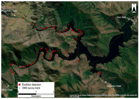
Figure 3.
Typical pattern of ebullition in a subtropical reservoir showing vessel track and location of detections across Borumba Dam in South East Queensland.
In temperate storages, such as Lake Gordon, the shallow water ebullition zones were primarily located in zones’ adjacent catchment inflows and along the shoreline of sub-basins within the reservoir (Figure 4). In addition, ebullition zones were found throughout the reservoir with activity detected near the dam wall (Figure 4). Lake Pedder followed a similar pattern to Lake Gordon with ebullition activity detected in adjacent catchment inflows and within shallow zones of sheltered sub-basins (Figure S15).
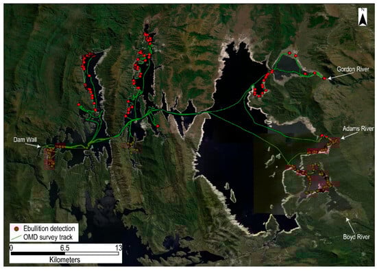
Figure 4.
Typical pattern of ebullition in a temperate reservoir showing vessel track and location of detections across Lake Gordon in Tasmania.
Ebullition activity in storages from both subtropical and temperate regions was generally confined to shallow zones, with the mean, median, and interquartile ranges in ebullition at water depths all less than 5 m (Figure 5). Significantly shallower ebullition water depths were found in temperate storages compared with subtropical storages (KW H(1,1941) = 224.0, p < 0.001) and median ebullition water depth was 1.3 m and 2.9 m, respectively (Figure 5).
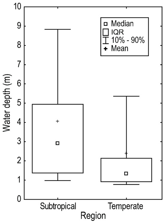
Figure 5.
Water depth of ebullition events detected across all studied temperate and subtropical water storages. Values indicate median and mean water depths with interquartile (IQR) and 10th to 90th percentile ranges.
In addition, a clear pattern for ebullition activity and water depth was observed across all 15 storages. In subtropical storages, over 75% of all ebullition detections were detected in water depths of less than 5 m (Figure 6A), and in temperate storages, this increased to over 90% of detections (Figure 6B). There was a steep reduction in ebullition detections with increasing water depth in both regions, where less than 3% and 1% of ebullition activity occurred below 15 m water depth in subtropical and temperate storages, respectively (Figure 6A,B). Maximum water depth of ebullition activity was over 50% deeper in subtropical storages (36.9 m) compared with temperate storages (23.3 m).
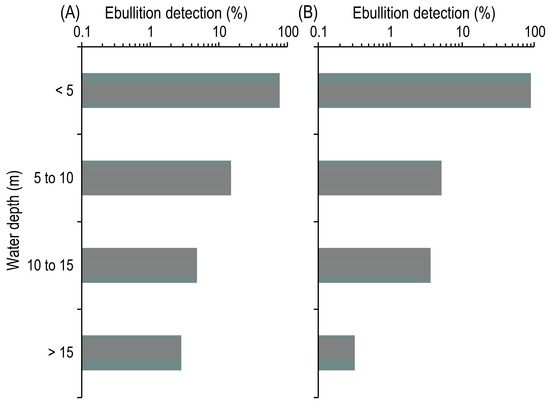
Figure 6.
Relationship between ebullition detection and water depth within (A) subtropical and (B) temperate storages. Please note ebullition detection percentage is visualised on log scale.
3.2. Equivalent Water Level as Ebullition Driver
Equivalent water level was demonstrated to be a driver of ebullition at spatial and temporal scales. Clear spatial changes in ebullition activity were observed within two sub-basins, Pearce and Holley Basins, on Lake Gordon during a period of dropping water levels in March 2022 (Figure 7A) and stable water levels in December 2022 (Figure 7B). The March 2022 surveys noted rapidly dropping water levels at approximately 10 cm per day (Figure 7A) during the field campaign, whilst in December 2022, water levels remained stable (Figure 7B). Considerable ebullition activity was observed in both sub-basins during dropping water levels, with over 100 ebullition detections (Figure 7C). Under stable equivalent water levels, ebullition detections were confined to a single zone in Pearce Basin, and no detections occurred in Holley Basin during this survey (Figure 7C).
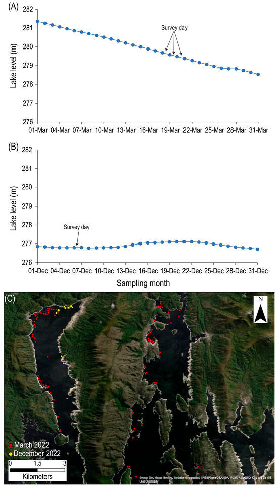
Figure 7.
Open-path, optical methane detector (OMD) surveys on Lake Gordon during (A) dropping and (B) stable water levels. (C) Location of ebullition detections in ebullition zones within Pearce and Holley Basins on Lake Gordon. Please sampling month in (A,B) are from 2022 calendar year.
Further evidence of spatial changes was observed in the ebullition zone of Lake Pedder, where two surveys were conducted within 3 days, with the first survey being conducted during increasing air pressure and the second survey during falling air pressure (Figure 8A). Ebullition activity was greatly reduced on the first survey day (5 December 2022) compared with the second survey (7 December 2022), with only two detections, whilst the second survey day identified 40 separate detections within the survey grid (Figure 8B). Water levels in Lake Pedder are relatively stable due to regulatory requirements, and during the December 2022 surveys, water level increased approximately 1 cm between surveys.
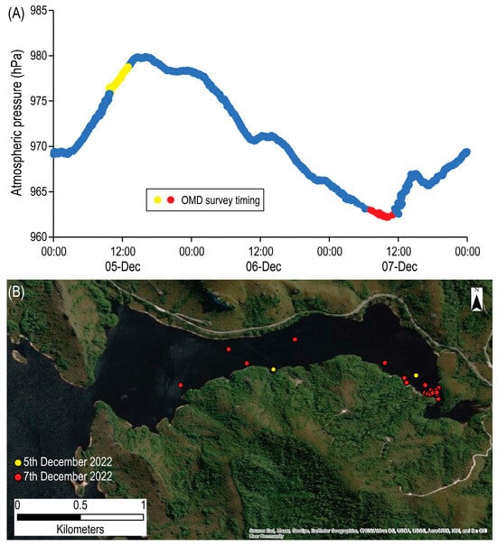
Figure 8.
(A) Atmospheric pressure changes in Lake Pedder during December 2022 field campaign, showing timing of OMD surveys. (B) Location of ebullition detections in a Lake Pedder ebullition zone (Holley Road embayment) from two surveys conducted on 5th and 7th December 2022.
Emission rates from ebullition zones of subtropical and temperate storages under dropping or stable equivalent water level showed a consistent pattern. The ebullitive flux rates in both subtropical (KW H(1,153) = 20.3, p < 0.001; Figure 9A) and temperate reservoirs (KW H(1,60) = 13.9, p < 0.001; Figure 9B) were significantly higher during dropping bed pressure conditions compared with stable or rising conditions. Median rates from across subtropical reservoirs under dropping sediment pressure conditions were approximately 4 times higher than rates during stable conditions (Figure 9A). Median rates from temperate reservoirs under dropping sediment pressure conditions were approximately 10 times higher than rates during stable conditions (Figure 9B). Mean emission rates were higher than median rates in both regions under dropping and stable conditions. Lower mean and median ebullition rates were observed in temperate storages compared with subtropical storages; however, the rates did not differ significantly (Figure 9A,B).
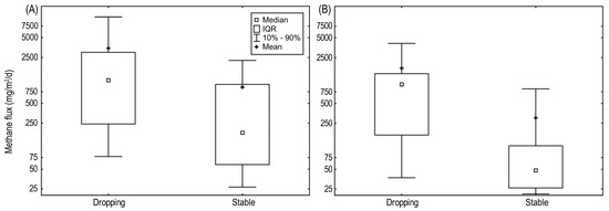
Figure 9.
Comparison of emission rates from ebullition zones in (A) subtropical and (B) temperate reservoirs during dropping or stable sediment bed pressure conditions. Values indicate median and mean emission rates with interquartile (IQR) and 10th to 90th percentile ranges. Please note methane flux rates are visualised on a log scale and refer only to areal rates and not total emissions from reservoirs.
4. Discussion
This study clearly demonstrated ebullition is a ubiquitous methane emission pathway in Australian subtropical and temperate storages. Ebullition activity was detected in all storages surveyed during this study, and the patterns of ebullition activity were strongly supported by previous research on subtropical and temperate reservoirs where shallow zones’ and depositional zones’ adjacent catchment inflows were hotspots for ebullition activity [4,13,14,24,26,27,28,29]. The depth distribution observed in ebullition activity is supported by the findings of [30], where up to 80% of ebullition occurred in depths of 4 m or less. This pattern has been observed in natural lakes where the probability of ebullition was demonstrated to be a function of depth, and zones greater than 6 m deep greatly reduced the likelihood of ebullition activity [31]. The spatial patterns of ebullition activity observed in both temperate reservoirs are consistent with studies in the subtropics where minor drops in water level and air pressure resulted in a major increase in ebullition area and activity [13,24]. The reduction in local sediment bed pressure during dropping equivalent water level is likely to initiate ebullition increasing both its rate and spatial extent [13,20]. These findings highlight the need to map zones of persistent ebullition activity within a water storage of interest, particularly to investigate shallow zones’ adjacent catchment inflows as these were repeatedly identified as ebullition zones across both regions.
The equivalent water level was clearly shown to be a driver of ebullition emission rates, with significantly higher rates observed during dropping conditions compared with stable conditions (Figure 9). Equivalent water level is likely to be driven by a combination of air pressure and water level (Figure 10), and understanding the relative change in both these variables will be the key to understanding emission estimates. Ebullition activity is significantly lower during conditions of increasing or stable equivalent water level where bubble release was restricted due to elevated effective pressure at the sediment-water interface. In turn, this reduction in ebullition activity allows the recharge of methane gas into the sediment void space. Under conditions of decreasing equivalent water level the effective pressure at the sediment-water interface is reduced and creates favourable conditions for bubble release (Figure 10). The influence of air pressure and water level changes on ebullition activity has been demonstrated in tropical and temperate reservoirs [32,33,34]. Dropping air pressure has been demonstrated as a driver of ebullition activity in arctic and temperate regions [35,36]. These findings highlight that both water level and air pressure changes are important drivers of ebullition activity in shallow zones of reservoirs. For example, in the subtropical reservoir, Sideling Creek Dam, over the 2017 annual cycle, water was dropping 86% of the time whilst air pressure was dropping only 21% of the time (Figure S16). However, the relative magnitude and timing of these changes in water level and air pressure were the local causes of sediment bed pressure changes, and by accounting for these results, equivalent water level dropped 71% of the time (Figure S16). To generate more confident estimates of ebullition emissions across the cycle, rates should be scaled using both dropping and stable equivalent water level conditions and the appropriate duration of filling and drawdown cycles in the reservoir.
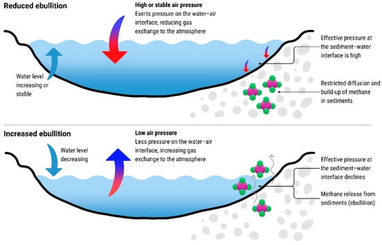
Figure 10.
Conceptual representation of the role of equivalent water level as a driver of ebullition activity.
Conceptually, the following steps emerge for both measurement and modelling techniques to develop spatially and temporally resolved estimation of emissions from water storages:
- Identify the temporal cycle that is appropriate for the reservoir. The duration of the hydrological cycle in the reservoirs in this study ranges from sub-annual to decadal.
- Identification of likely zones of ebullition: This is informed by bathymetry and likely depositional areas. If a measurement approach is adopted, surveillance methods (for example, OMD) should be used to confirm ebullition under favourable equivalent water level conditions (stable, falling water levels and air pressures). This mapping will allow the identification of suitable deployment sites that cover the key reservoir zones and their relative surface area.
- Quantification of areal emissions rates: It is suggested these key reservoir zones are separated based on the water depth categories identified in Figure 6. To overcome the challenge of spatial weighting within the key zones, chamber deployments can be undertaken within each zone to estimate areal emission rates. Total reservoir emissions will, therefore, be a function of the key zone relative surface area and chamber derived emission rates for that zone. A conceptual representation of this approach is provided in Figure 11 illustrating the importance of representative areal emission rates from ebullition zones in determining total storage emissions.
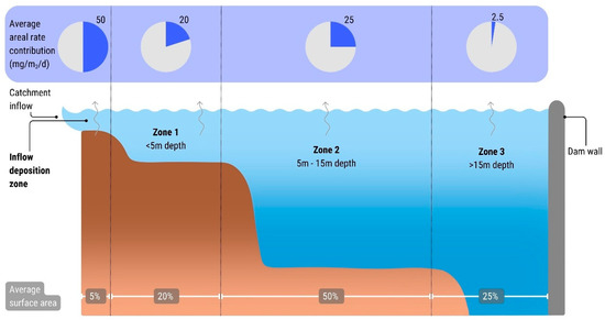 Figure 11. Conceptual representation of key monitoring zones within a water storage showing the relative contribution to total inundation zone emissions using idealised areal emission rates from each zone.
 - Identification of equivalent water level conditions that favour ebullition: This will require consideration of hydrological cycle (item 1), water depth, and air pressure conditions. The coincidence of falling water levels and falling air pressures is likely to be the most favourable for ebullition.
- Integration of spatially weighted areal emissions with the appropriate temporal resolution for the reservoir to derive spatially and temporally resolved estimation of ebullition emissions.
Ebullition will be sensitive to water level or air pressure changes if the sediments void spaces have sufficient pressure to overcome the hydrostatic pressure. If the sediment void spaces have been exhausted, either due to large drops in the hydrostatic pressure or prolonged conditions favouring ebullition, then subsequent pressure changes will not result in ebullition until the sediment void spaces again accumulate sufficient methane.
One final consideration lies in the choice of the measure of centrality to develop representative emission rates. In the subtropical storages investigated in this study, the mean emission rate was more than double the median emission rate under dropping and stable conditions. A similar pattern was observed in temperate reservoirs, and this represents an important challenge to researchers and industry practitioners in determining total emission estimates. This raises a key issue in estimating ebullition rates from water storages as log-normal data distributions are likely due to highly elevated rates obtained in very few replicates [24]. We recommend consistency in reporting both measures of centrality, as this range is likely to provide a representative estimate of emission rates; however, the median rate is likely to approximate a globally relevant rate [28,37].
5. Conclusions
In conclusion, this study demonstrated that dropping equivalent water level increased ebullition activity across 15 subtropical and temperate water storages. Therefore, it is important to quantify emission rates of ebullition zones under dropping and stable equivalent water levels to improve confidence in total methane emission estimates of Australian water storages. Noteworthily, although this study covered approximately 10% of Australia’s flooded land surface area, there were only 15 systems monitored out of 1020 reservoirs in the country (National Surface Hydrology); thus, future studies will be required to refine our understanding of the patterns of ebullition activity. Moreover, further research is required globally to investigate the concept of equivalent water level across a range of reservoir types and sediment characteristics to inform the development of qualitative and quantitative estimation techniques that enable spatially and temporally resolved emission estimates.
The development of robust methods for estimating emissions from reservoirs is important for corporations and governments globally. The adoption of the Paris Agreement and the widespread adoption of carbon accounting standards [38] have resulted in greater transparency of national and corporate emission profiles. As governments and corporations invest in reducing carbon emissions, inaccuracies caused by carbon estimation methods can result in financial and reputation losses and other consequences for the parties involved, and this has resulted in greater transparency of national and corporate emission profiles.
Supplementary Materials
The following supporting information can be downloaded at: https://www.mdpi.com/article/10.3390/app15179795/s1, Table S1: Water storage name and location of ebullition zones for chamber deployments in 13 reservoirs and 2 weirs. Figure S1: Study area of thirteen subtropical water storages relative to South East Queensland and Australia (inset). Figure S2: Study area of two temperate water storages relative to South West Tasmania and Australia (inset). Figure S3: Pattern of ebullition in a subtropical reservoir showing locations of bubble detections across Baroon Pocket Dam in South East Queensland. Figure S4: Pattern of ebullition in a subtropical weir showing locations of bubble detections across Mt Crosby Weir in South East Queensland. Figure S5: Pattern of ebullition in a subtropical reservoir showing locations of bubble detections across Enoggera Dam in South East Queensland. Figure S6: Pattern of ebullition in a subtropical reservoir showing locations of bubble detections across Gold Creek Dam in South East Queensland. Figure S7: Pattern of ebullition in a subtropical reservoir showing locations of bubble detections across Lake Manchester in South East Queensland. Figure S8: Pattern of ebullition in a subtropical reservoir showing locations of bubble detections across Little Nerang Dam in South East Queensland. Figure S9: Pattern of ebullition in a subtropical reservoir showing locations of bubble detections across North Pine Dam in South East Queensland. Figure S10: Pattern of ebullition in a subtropical weir showing locations of bubble detections across O’Reilly’s Weir in South East Queensland. Figure S11: Pattern of ebullition in a subtropical reservoir showing locations of bubble detections across Sideling Creek Dam in South East Queensland. Figure S12: Pattern of ebullition in a subtropical reservoir showing locations of bubble detections across Somerset Dam in South East Queensland. Figure S13: Pattern of ebullition in a subtropical reservoir showing locations of bubble detections across Lake Wivenhoe in South East Queensland. Figure S14: Pattern of ebullition in a subtropical reservoir showing locations of bubble detections across Wyaralong Dam in South East Queensland. Figure S15: Pattern of ebullition in a temperate reservoir showing locations of bubble detections across Lake Pedder in South West Tasmania. Figure S16: (A) Annual water level and air pressure from Sideling Creek Dam in South East Queensland. (B) Annual equivalent water level derived from the combination of water level and air pressure.
Author Contributions
Conceptualization, A.G. and C.M.; methodology, A.G. and K.S.; validation, C.M. and R.R.; formal analysis, A.G. and C.M.; investigation, C.M., L.H. and A.G.; writing—original draft preparation, A.G., K.S., C.M. and L.H.; writing—review and editing, L.H. and R.R.; funding acquisition, C.M., K.S. and A.G. All authors have read and agreed to the published version of the manuscript.
Funding
This research was supported by Hydro-Electric Corporation and Seqwater.
Institutional Review Board Statement
Not applicable.
Informed Consent Statement
Not applicable.
Data Availability Statement
Data supporting reported results can be found in the Supplementary Materials.
Acknowledgments
Kevin McFarlane, Brendon Duncan, and Nathaniel Deering are gratefully acknowledged for their field and logistical support. Melanie Johnson and Andy Taylor are gratefully acknowledged for their spatial analysis and conceptual model development. We gratefully acknowledge the four reviewers for their constructive comments and suggestions.
Conflicts of Interest
Authors Carolyn Maxwell and Luke Hickman were employed by the company Hydro Tasmania. Authors Katrin Sturm and Rodney Ringe were employed by the company Seqwater. The remaining author declare that the research was conducted in the absence of any commercial or financial relationships that could be construed as a potential conflict of interest.
References
- 2019 Refinement to the 2006 IPCC Guidelines for National Greenhouse Gas Inventories, Volume 4, Agriculture, Forestry and Other Land Use. Available online: https://www.ipcc-nggip.iges.or.jp/public/2019rf/vol4.html (accessed on 16 April 2025).
- Johnson, M.S.; Matthews, E.; Bastviken, D.; Deemer, B.; Du, J.; Genovese, V. Spatiotemporal methane emission from global reservoirs. J. Geophys. Res. Biogeosci. 2021, 126, 2. [Google Scholar] [CrossRef]
- Deemer, B.R.; Harrison, J.A.; Li, S.; Beaulieu, J.J.; DelSontro, T.; Barros, N.; Bezerra-Neto, J.F.; Powers, S.M.; Dos Santos, M.A.; Vonk, J.A. Greenhouse gas emissions from reservoir water surfaces: A new global synthesis. BioScience 2016, 66, 949–964. [Google Scholar] [CrossRef] [PubMed]
- Beaulieu, J.J.; Waldo, S.; Balz, D.A.; Barnett, W.; Hall, A.; Platz, M.C.; White, K.M. Methane and carbon dioxide emissions from reservoirs: Controls and upscaling. J. Geophys. Res. Biogeosci. 2020, 125, e2019JG005474. [Google Scholar] [CrossRef] [PubMed]
- Harrison, J.A.; Prairie, Y.T.; Mercier-Blais, S.; Soued, C. Year-2020 global distribution and pathways of reservoir methane and carbon dioxide emissions according to the greenhouse gas from reservoirs (G-res) model. Glob. Biogeochem. Cycles 2021, 35, e2020GB006888. [Google Scholar] [CrossRef]
- Sturm, K.; Keller-Lehmann, B.; Werner, U.; Raj Sharma, K.; Grinham, A.R.; Yuan, Z. Sampling considerations and assessment of Exetainer usage for measuring dissolved and gaseous methane and nitrous oxide in aquatic systems. Limnol. Oceanogr. Methods 2015, 13, 375–390. [Google Scholar] [CrossRef]
- Hofmann, H.; Federwisch, L.; Peeters, F. Wave-induced release of methane: Littoral zones as source of methane in lakes. Limnol. Oceanogr. 2010, 55, 1990–2000. [Google Scholar] [CrossRef]
- Bogard, M.J.; Del Giorgio, P.A.; Boutet, L.; Chaves, M.C.G.; Prairie, Y.T.; Merante, A.; Derry, A.M. Oxic water column methanogenesis as a major component of aquatic CH4 fluxes. Nat. Commun. 2014, 5, 5350. [Google Scholar] [CrossRef]
- Soued, C.; Prairie, Y.T. Patterns and regulation of hypolimnetic CO2 and CH4 in a tropical reservoir using a process-based modeling approach. J. Geophys. Res. Biogeosci. 2022, 127, e2022JG006897. [Google Scholar] [CrossRef]
- Bastviken, D.; Tranvik, L.J.; Downing, J.A.; Crill, P.M.; Enrich-Prast, A. Freshwater methane emissions offset the continental carbon sink. Science 2011, 331, 50. [Google Scholar] [CrossRef]
- Wik, M.; Johnson, J.E.; Crill, P.M.; DeStasio, J.P.; Erickson, L.; Halloran, M.J.; Fahnestock, M.F.; Crawford, M.K.; Phillips, S.C.; Varner, R.K. Sediment characteristics and methane ebullition in three subarctic lakes. J. Geophys. Res. Biogeosci. 2018, 123, 2399–2411. [Google Scholar] [CrossRef]
- Aben, R.C.; Barros, N.; Van Donk, E.; Frenken, T.; Hilt, S.; Kazanjian, G.; Lamers, L.P.; Peeters, E.T.; Roelofs, J.G.; de Senerpont Domis, L.N.; et al. Cross continental increase in methane ebullition under climate change. Nat. Commun. 2017, 8, 1682. [Google Scholar] [CrossRef]
- Grinham, A.; Dunbabin, M.; Gale, D.; Udy, J. Quantification of ebullitive and diffusive methane release to atmosphere from a water storage. Atmos. Environ. 2011, 45, 7166–7173. [Google Scholar] [CrossRef]
- Joyce, J.; Jewell, P.W. Physical controls on methane ebullition from reservoirs and lakes. Environ. Eng. Geosci. 2003, 9, 167–178. [Google Scholar] [CrossRef]
- Kellner, E.; Baird, A.J.; Oosterwoud, M.; Harrison, K.; Waddington, J.M. Effect of temperature and atmospheric pressure on methane (CH4) ebullition from near-surface peats. Geophys. Res. Lett. 2006, 33, L18405. [Google Scholar] [CrossRef]
- Grinham, A.; Dunbabin, M.; Albert, S. Importance of sediment organic matter to methane ebullition in a sub-tropical freshwater reservoir. Sci. Total Environ. 2018, 621, 1199–1207. [Google Scholar] [CrossRef]
- Surface Hydrology Polygons (National). Available online: https://ecat.ga.gov.au/geonetwork/srv/eng/catalog.search#/metadata/83135 (accessed on 2 February 2025).
- Lehner, B.; Liermann, C.R.; Revenga, C.; Vörösmarty, C.; Fekete, B.; Crouzet, P.; Döll, P.; Endejan, M.; Frenken, K.; Magome, J. High-resolution mapping of the world’s reservoirs and dams for sustainable river-flow management. Front. Ecol. Environ. 2011, 9, 494–502. [Google Scholar] [CrossRef]
- Dunbabin, M.; Grinham, A. Quantifying spatiotemporal greenhouse gas emissions using autonomous surface vehicles. J. Field Robot. 2017, 4, 151–169. [Google Scholar] [CrossRef]
- Varadharajan, C.; Hemond, H.F. Time-series analysis of high-resolution ebullition fluxes from a stratified, freshwater lake. J. Geophys. Res. Biogeosci. 2012, 117, G02004. [Google Scholar] [CrossRef]
- Water Data Online. Available online: www.bom.gov.au/waterdata/ (accessed on 15 March 2025).
- Climate Data Online. Available online: www.bom.gov.au/climate/data/ (accessed on 15 March 2025).
- Berglund, Ö.; Berglund, K. Influence of water table level and soil properties on emissions of greenhouse gases from cultivated peat soil. Soil Biol. Biochem. 2011, 43, 923–931. [Google Scholar] [CrossRef]
- Grinham, A.; Albert, S.; Deering, N.; Dunbabin, M.; Bastviken, D.; Sherman, B.; Lovelock, C.E.; Evans, C.D. The importance of small artificial water bodies as sources of methane emissions in Queensland, Australia. Hydrol. Earth Sys. Sci. 2018, 22, 5281–5298. [Google Scholar] [CrossRef]
- Dell Inc. 2016. Available online: http://www.statsoft.com/Products/STATISTICA-Features (accessed on 20 April 2025).
- Beaulieu, J.J.; McManus, M.G.; Nietch, C.T. Estimates of reservoir methane emissions based on a spatially balanced probabilistic-survey. Limnol. Oceanogr. 2016, 61, S27–S40. [Google Scholar] [CrossRef]
- de Mello, N.A.S.T.; Brighenti, L.S.; Barbosa, F.A.R.; Staehr, P.A.; Bezerra Neto, J.F. Spatial variability of methane (CH4) ebullition in a tropical hypereutrophic reservoir: Silted areas as a bubble hot spot. Lake Reserv. Manag. 2018, 34, 105–114. [Google Scholar] [CrossRef]
- Hansen, C.H.; Iftikhar, B.; Pilla, R.M.; Griffiths, N.A.; Matson, P.G.; Jager, H.I. Temporal variability in reservoir surface area is an important source of uncertainty in GHG emission estimates. Water Resour. Res. 2025, 61, e2024WR037726. [Google Scholar] [CrossRef]
- Shi, W.; Chen, Q.; Zhang, J.; Lu, J.; Chen, Y.; Pang, B.; Yu, J.; Van Dam, B.R. Spatial patterns of diffusive methane emissions across sediment deposited riparian zones in hydropower reservoirs. J. Geophys. Res. Biogeosci. 2021, 126, e2020JG005945. [Google Scholar] [CrossRef]
- Bastviken, D.; Cole, J.; Pace, M.; Tranvik, L. Methane emissions from lakes: Dependence of lake characteristics, two regional assessments, and a global estimate. Glob. Biogeochem. Cycles 2004, 18, GB4009. [Google Scholar] [CrossRef]
- West, W.E.; Creamer, K.P.; Jones, S.E. Productivity and depth regulate lake contributions to atmospheric methane. Limnol. Oceanogr 2016, 61, S51–S61. [Google Scholar] [CrossRef]
- Keller, M.; Stallard, R.F. Methane emission by bubbling from Gatun Lake, Panama. J. Geophys. Res. Atmos. 1994, 99, 8307–8319. [Google Scholar] [CrossRef]
- Wik, M.; Crill, P.M.; Bastviken, D.; Danielsson, Å.; Norbäck, E. Bubbles trapped in arctic lake ice: Potential implications for methane emissions. J. Geophys. Res. Biogeoscie. 2011, 116, G03044. [Google Scholar] [CrossRef]
- Maeck, A.; Hofmann, H.; Lorke, A. Pumping methane out of aquatic sediments–ebullition forcing mechanisms in an impounded river. Biogeosciences 2014, 11, 2925–2938. [Google Scholar] [CrossRef]
- Mattson, M.D.; Likens, G.E. Air pressure and methane fluxes. Nature 1990, 347, 718–719. [Google Scholar] [CrossRef]
- Wik, M.; Crill, P.M.; Varner, R.K.; Bastviken, D. Multiyear measurements of ebullitive methane flux from three subarctic lakes. J. Geophys. Res. Biogeosci. 2013, 118, 1307–1321. [Google Scholar] [CrossRef]
- Rosentreter, J.A.; Borges, A.V.; Deemer, B.R.; Holgerson, M.A.; Liu, S.; Song, C.; Melack, J.; Raymond, P.A.; Duarte, C.M.; Allen, G.H.; et al. Half of global methane emissions come from highly variable aquatic ecosystem sources. Nat. Geosci. 2021, 14, 225–230. [Google Scholar] [CrossRef]
- International Sustainability Standards Board (ISSB). IFRS S2 climate-related Disclosures; IFRS Foundation: London, UK, 2023; Available online: https://www.ifrs.org/issued-standards/ifrs-sustainability-standards-navigator/ifrs-s2-climate-related-disclosures/ (accessed on 25 August 2025).
Disclaimer/Publisher’s Note: The statements, opinions and data contained in all publications are solely those of the individual author(s) and contributor(s) and not of MDPI and/or the editor(s). MDPI and/or the editor(s) disclaim responsibility for any injury to people or property resulting from any ideas, methods, instructions or products referred to in the content. |
© 2025 by the authors. Licensee MDPI, Basel, Switzerland. This article is an open access article distributed under the terms and conditions of the Creative Commons Attribution (CC BY) license (https://creativecommons.org/licenses/by/4.0/).