Article

The Potential of U-Net in Detecting Mining Activity: Accuracy Assessment Against GEE Classifiers

by
Beata Hejmanowska
*,†,
Krystyna Michałowska
,
Piotr Kramarczyk
and
Ewa Głowienka
AGH University of Krakow, Faculty of Geo-Data Science, Geodesy and Environmental Engineering, Department of Photogrammetry Remote Sensing of Environment and Spatial Engineering, al. A. Mickiewicza 30, 30-059 Krakow, Poland
*
Author to whom correspondence should be addressed.
These authors contributed equally to this work.
Appl. Sci. 2025, 15(17), 9785; https://doi.org/10.3390/app15179785 (registering DOI)
Submission received: 16 July 2025 / Revised: 24 August 2025 / Accepted: 25 August 2025 / Published: 5 September 2025

Abstract

Illegal mining poses significant environmental and economic challenges, and effective monitoring is essential for regulatory enforcement. This study evaluates the potential of the U-Net deep learning model for detecting mining activities using Sentinel-2 satellite imagery over the Strzegom region in Poland. We prepared annotated datasets representing various land cover classes, including active and inactive mineral extraction sites, agricultural areas, and urban zones. U-Net was trained and tested on these data, and its classification accuracy was assessed against common Google Earth Engine (GEE) classifiers such as Random Forest, CART, and SVM. Accuracy metrics, including Overall Accuracy, Producer’s Accuracy, and F1-score, were computed. Additional analyses compared model performance for detecting licensed versus potentially illegal mining areas, supported by integration with publicly available geospatial datasets (MOEK, MIDAS, CORINE). The results show that U-Net achieved higher detection accuracy for mineral extraction sites than the GEE classifiers, particularly for small and spatially heterogeneous areas. This approach demonstrates the feasibility of combining deep learning with open geospatial data for supporting mining activity monitoring and identifying potential cases of unlicensed extraction.

1. Introduction

Illegal mineral exploitation is both unlawful and highly detrimental, causing significant financial losses and environmental degradation. Different countries are attempting to monitor this phenomenon through various approaches, achieving mixed levels of success. Against this backdrop, we outline the methods and datasets currently in use, alongside the shortcomings and gaps in existing monitoring frameworks. Finally, we introduce our research as a contribution towards addressing these deficiencies, highlighting the scope and innovative aspects of our approach.
Unauthorized open-pit mineral extraction, while economically beneficial for its operators, poses serious threats to the environment, public health, and sustainable development. It leads to deforestation, habitat destruction, soil and water pollution, and undermines land reclamation efforts that are critical for restoring ecological balance. Moreover, unauthorized mining bypasses legal regulations, resulting in mineral theft, environmental degradation, and financial losses for local governments. In Poland alone, between 2015 and 2023, over 3000 cases of illegal mining were reported, with total fines exceeding USD 52 million [1,2]. The growing demand for construction aggregates—such as sand, gravel, dolomite, and limestone—due to recent infrastructure expansion has increased the risk of unregulated extraction. While all mining activities are subject to national geological and environmental laws, enforcement remains difficult due to limited accessibility, unknown locations, and the vast extent of potential mining sites, making traditional field-based monitoring expensive and inefficient.
Remote sensing has emerged as an effective approach for detecting and monitoring illegal or informal mining in regions where this practice is carried out on a large scale Table 1 and Table 2. Optical time series from Landsat8/9 and Sentinel-2 allow mapping of deforestation fronts, open pits, tailings, and sediment plumes in river systems, while SAR data (Sentinel-1) provide all-weather capabilities for detecting changes in surface roughness and coherence linked to earthworks and slope instability. Recent advances also exploit very-high-resolution (VHR) and PlanetScope imagery for near-real-time alerts, deep learning for semantic segmentation, and integrated optical–SAR workflows to ensure robust classification under continuous cloud cover [3,4,5,6,7,8,9].
Key methodological strands include the following [10]: (1) time-series change detection using vegetation and water indices (e.g., NDVI, NDMI, NDWI/MNDWI) to track expansion of mining pads [1,4,11,12]; (2) SAR for cloud-prone regions and stability monitoring, where amplitude/texture metrics and interferometric analyses reveal site activation beneath cloud cover and enable detection of slope or tailings instability [13,14]; (3) deep learning segmentation with U-Net/FCN models trained on Sentinel-2 and Planet imagery, enhancing delineation of mining areas and enabling cross-basin transfer through careful domain adaptation [5]; (4) data fusion, as demonstrated in large-scale Indonesian studies, where combining multispectral (Landsat/S2) and radar (S1/ALOS PALSAR) data within GEE workflows increases classification accuracy [6,15].
Table 1. Comparison of remote sensing methods for detecting illegal or informal mining in selected regions where this practice is carried out on a large scale (Part 1: sensor, signal, task; rows continued in Table 2).
IDSensor/DataSignal/IndexPrimary Task
1Landsat 8/9, Sentinel-2NDVI, NDMI, NDWI/MNDWI, time seriesDetect deforestation fronts, open pits, river sediment plumes
2PlanetScope (3–5 m) VHRTrue color, texture, plume extentNear-operational hotspot mapping
3Sentinel-1 SARAmplitude/texture change, coherence loss, DInSARAll-weather detection of pits, slope instability
4Optical + SAR fusion (S2 + S1, ALOS PALSAR)Multispectral + backscatterLarge-area mapping of disturbed surfaces
5Airborne LiDAR + VHRElevation change, canopy removalQuantify carbon loss; detect micro-features
6Deep learning segmentation (U-Net, FCN)Spectral + spatial patternsSemantic segmentation of mining/tailings
7Nighttime lights (VIIRS/DNB)Radiance anomaliesProxy detection of mining camp activity through nighttime light patterns
Table 2. Comparison of remote sensing methods for detecting illegal or informal mining in selected regions where this practice is carried out on a large scale (Part 2: pros, cons, accuracy, country; rows are a continuation of Table 1).
IDProsCons/LimitationsReported AccuracyCountry
1Long-term archive; free/open; large AOIsCloud cover; 10–30 m may miss small sitesOA 85–92%, F1 ∼0.80–0.88Peru, Venezuela, Indonesia [3,4,6,11,12,13,16,17]
2High spatial detail; daily revisitCommercial; limited historyVisual confirmation, >90% correct IDPeru, Venezuela [3,4,11,12,16,17]
3Cloud-independent; sensitive to roughness/moistureLower thematic specificity without opticalOA ∼82%, F1 ∼0.78Indonesia, Myanmar [6,13,18]
4Complements sensor limits; better under mixed conditionsCo-registration; complex processingOA up to 94%, F1 ∼0.90Indonesia [6,13,18,19]
5High accuracy; 3D capabilityExpensive; limited coverageRMSE ∼0.15 m; >99% detection pits >0.02 haPeru [3,4,11,12]
6High delineation accuracy; transferable modelsNeeds large training setsOA 92–96%, F1 ∼0.91–0.94Peru, Indonesia [3,4,6,11,12,13,18]
7Cloud-independent; unaffected by vegetation coverLow resolution; light sources from settlements or fires may confound interpretationnot availableCross-regional (tropics)
Undoubtedly, the dominant method is automatic image classification, including machine learning techniques and neural networks, including deep learning. Deep learning has transformed remote sensing image analysis. CNNs [20,21] extract spatial–spectral features but often require large datasets. FCNs [22], SegNet [23], and DeepLab [24] extend pixel-wise segmentation with higher accuracy. Among them, U-Net [25] is widely used [26,27] due to its skip connections and strong performance with small datasets.
Recently, Transformer-based architectures have gained increasing attention in remote sensing, owing to their ability to model long-range dependencies and temporal dynamics more effectively than conventional CNNs or RNNs. For instance, Garnot et al. [28] introduced the Pixel-Set Encoder with temporal self-attention to handle irregular Sentinel-2 time series, while other studies proposed dual-attention CNNs or hybrid CNN–RNN frameworks with attention to improve robustness against data gaps and spectral variability [29,30]. More recently, dedicated architectures such as FCIHMRT (Fully Convolutional Image Hierarchical Multi-scale Remote-sensing Transformer) have been applied to land cover mapping, demonstrating that self-attention can capture both spectral and spatial dependencies across scales with state-of-the-art performance.
Recently, Transformer-based architectures have gained increasing attention in remote sensing due to their ability to model long-range dependencies and temporal dynamics more effectively than conventional CNNs or RNNs. For example, Garnot et al. [28] introduced the Pixel-Set Encoder with temporal self-attention to handle irregular Sentinel-2 time series, while other studies proposed dual-attention CNN or hybrid CNN–RNN frameworks with attention to improve robustness against data gaps and spectral variability [29,30]. More recently, dedicated architectures such as FCIHMRT (Feature Cross-Layer Interaction Hybrid Method based on Res2Net and Transformer) have been applied to land cover mapping, demonstrating that self-attention can capture both spectral and spatial dependencies across scales with state-of-the-art performance [31].
In this context, our study deliberately adopts a U-Net-based approach integrated with Google Earth Engine (GEE) classifiers. Although Transformer models show great potential, they typically require larger datasets and higher computational resources. In contrast, U-Net offers a lightweight yet robust architecture that can be trained on moderate datasets and deployed efficiently on operational platforms. This choice reflects our aim of developing a workflow that is not only accurate but also accessible to practitioners and scalable across regions with limited resources.
Example applications of neural networks in LULC classification in agricultural areas are presented in Table 3. The table summarizes selected studies applying neural networks to LULC classification in agricultural areas using Sentinel-2 time series data. The examples illustrate the evolution from early CNN-based approaches, such as EuroSAT, toward more advanced architectures integrating temporal information, attention mechanisms, and gap-handling strategies. Reported results show that recurrent and attention-based models generally outperform classical machine learning methods, achieving high Overall Accuracy and enabling earlier and more reliable crop identification. These studies highlight the growing role of deep learning in improving LULC monitoring from satellite imagery.
In our study, we adopt the U-Net architecture for several reasons: it performs efficiently on moderate hardware, is robust to seasonal variability, and can reliably distinguish mining areas from spectrally similar classes. U-Net was also chosen because our training dataset was relatively limited, making a compact yet powerful model more suitable, and because it offers a straightforward design that is easy to implement and operate, even by non-specialists. Our objective is to train the model once, without the need for retraining, and then apply it to other regions of Poland using multiseason Sentinel-2 imagery. This work represents an initial step toward a generalized, no-additional-training workflow, intended for operational monitoring and user-friendly deployment in platforms such as GEE.
Apart from selecting the neural network model, two issues still remain to be addressed:
  • Standard LULC datasets often lack dedicated mining classes [36];
  • Accuracy reporting is inconsistent, with some studies inflating metrics by using per-class accuracy instead of Overall Accuracy [37,38,39,40].
The main contributions of our study are summarized below to clearly present its novelty and value:
  • Proposing a mining-aware LULC classification scheme that incorporates seasonally distinct crop phases and explicitly introduces a dedicated quarry class;
  • Developing a workflow that integrates U-Net deep learning with Google Earth Engine classifiers, and emphasizes the importance of proper accuracy metric interpretation in imbalanced datasets;
  • Demonstrating the applicability of the proposed workflow for detecting and mapping potentially illegal mining sites by combining remote sensing classification with open geospatial datasets.

2. Materials and Methods

The primary objective of this study was to assess whether a convolutional neural network can accurately classify land use and land cover (LULC) types for the purpose of delineating mining areas. The model was designed to operate on a single Sentinel-2 image acquired at any time of the year—excluding periods of snow cover—without using any training data from the tested locations.
A fundamental problem in machine learning is the availability of benchmarks. Therefore, the first part of this Section 2.1 presents the benchmark datasets for the test site currently available, followed by a description of our own approach in Section 2.2 entitled Proposed Mining-Aware LULC Scheme.
Section 2.3 discusses the classification method: primarily U-Net, but also Random Forest (RF), Support Vector Machine (SVM), and CART, implemented using the cloud-based platform Google Earth Engine.
Section 2.4 includes the dataset used for U-Net classification and the codes and data used within the Google Earth Engine (GEE) platform. The following resources are publicly available [accessed on 29 July 2025]:
Section 2.5 addresses the accuracy metrics. Due to certain ambiguities surrounding this topic, it provides comprehensive information on how accuracy metrics are calculated, including a numerical example.
Since commonly available tools—both “ready-to-use” (e.g., QGIS, SAGA, PCI, ENVI) and programming libraries (e.g., scikit-learn)—offer only a limited subset of metrics that are historically aligned either with remote sensing or with machine learning, a custom script was used. Our script, which is publicly available, allows for the calculation of all accuracy metrics using various types of input data: accuracy_checker v.2.0.0 GitHub repository (https://github.com/python-edu/accuracy_checker) [accessed on 29 July 2025].

2.1. Test Site and Benchmarks

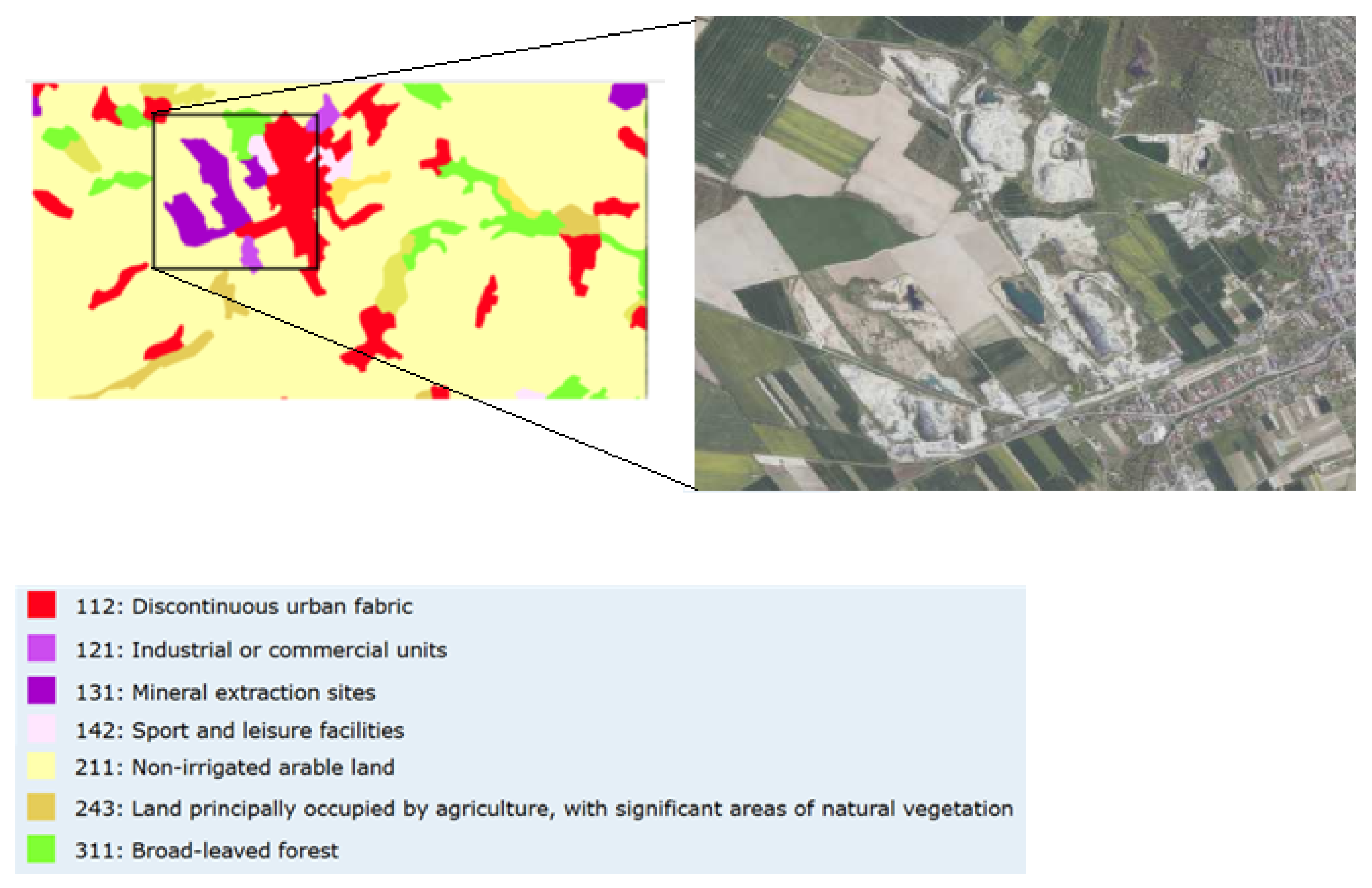
To this end, the study was conducted in three regions in Poland (gios.gov.pl (https://clc.gios.gov.pl/index.php/geoportal, accessed on 24 August 2025)) with contrasting land use profiles (geoportal.gov.pl (https://mapy.geoportal.gov.pl/imap/Imgp_2.html?locale=pl&gui=new&sessionID=CA163811-1BA2-4CED-8056-E6DC127C6D38, accessed on 24 August 2025)): Strzegom (a granite mining area in Lower Silesia), Kolbuszowa (an agricultural region in the Subcarpathian Plain), and Kraków (an urban and peri-urban area), Figure 1. The test areas were used first in our previous research [41].
Sentinel-2 Level-2A imagery from 2019 to 2023 was used. Ten spectral bands (B2, B3, B4, B5, B6, B7, B8, B8A, B11, and B12) were utilized, all resampled to a spatial resolution of 10 m. A similar approach—employing multiple heterogeneous test areas to improve classification generalization—was adopted in other recent studies [42,43].
All methods for detecting illegal mining sites require manual intervention in the computational process. Using indices involves specifying thresholds to separate LULC categories or distinguishing exploitation areas from the background in binary classification. Machine learning methods applied to illegal excavation recognition require a large training dataset. Acquiring reference data for machine learning is very time-consuming and costly, especially since machine learning requires a large amount of training data, which constitute the majority of all reference data. In recent years, several new reference datasets for LULC classification have emerged. The division of existing LULC (land use land cover) benchmarks used in machine learning, based on the level of detail in the defined classes, is as follows:
1.
Level-1 detail, characterized by general categories covering basic types of land use and cover:
(a)
EuroSAT 2018 [32]
  • Ten classes: industrial, pasture, river, forest, annual crop, permanent crop, highway, herbaceous vegetation, residential, sea lake.
  • Ten countries: Austria, Belgium, Finland, Ireland, Kosovo, Lithuania, Luxembourg, Portugal, Serbia, and Switzerland.
(b)
LandCoverNet 2020 [44,45]
  • Seven classes: snow/ice, water, bare ground artificial, bare ground natural, woody, vegetation cultivated, vegetation semi-natural.
  • Scope: Global.
2.
Level-3 detail covers more detailed categories of land use and cover:
(a)
BigEarthNet v2.0 2024 [46,47]
  • Nineteen classes.
  • Ten countries: the same as those included in EuroSAT.
(b)
MultiSenNA 2024 [48,49]
  • Fourteen classes.
  • Area: Eastern part of France.
(c)
SEASONET [50,51]
  • Thirty-three classes.
  • Area: Germany.

2.1.1. Limitations of Existing LULC Datasets for Mapping Mineral Extraction Sites in Poland

Despite the availability of several high-quality annotated LULC datasets such as EuroSAT, BigEarthNet, MultiSenNA, or SEASONET, their direct applicability to mapping mineral extraction sites in Poland is limited.
Firstly, datasets at Level-1 detail (e.g., EuroSAT and LandCoverNet) do not include a dedicated class for open-pit mines. Their primary focus is on general land use categories (e.g., forest, water, cropland), which do not allow the model to differentiate between legal and illegal resource extraction areas. Furthermore, the geographic coverage of these datasets is often restricted to Western or Central Europe, and does not include Poland.
In contrast, Level-3 datasets, such as BigEarthNet v2.0, MultiSenNA, or SEASONET, offer finer class granularity (14–33 classes), with some including mining-related categories. However, the limitations are as follows:
  • BigEarthNet lacks any class directly corresponding to mineral extraction.
  • MultiSenNA and SEASONET do include such classes, namely Class 12–Open Space, Mineral and Class 7–Mineral Extraction Sites, respectively, but they are geographically restricted (France and Germany) and not calibrated for Polish landscapes.
Furthermore, these datasets are based on Sentinel-2 patches of limited size (e.g., 64 × 64 px) and require significant preprocessing before use in pixel-wise segmentation tasks.
In light of these limitations, we also examined the CORINE Land Cover (CLC) database, which is one of the most widely used LULC datasets in Europe. Although CORINE provides detailed hierarchical classification (up to 44 classes at Level 3), including Class 131–Open-pit mining areas, it is not specifically designed for use in satellite image classification tasks involving machine learning.
Its primary purpose is to support environmental reporting and land management on national and continental scales, with thematic maps updated every few years. Moreover, the relatively coarse spatial resolution and vector-based format of CORINE data make it less suitable for direct integration into pixel-wise deep learning pipelines. As such, while CORINE served as a reference to illustrate existing class taxonomies, it could not be adopted as a benchmark for training or validating our models.

2.1.2. CORINE

The land cover classes in the CORINE Land Cover (CLC) program are hierarchically organized into three levels (gios.gov.pl (https://clc.gios.gov.pl/index.php/geoportal, accessed on 24 August 2025)):
  • Level 1 encompasses five main land cover types: artificial surfaces, agricultural areas, forests and semi-natural ecosystems, wetlands, and water bodies.
  • Level 2 differentiates 15 land cover forms.
  • Level 3 specifies 44 classes.
This level of detail has been applied to the development of land cover databases in all European countries. In Poland, of the 44 land cover classes, 31 classes are present, including Class 131—Mineral extraction sites. At Level 2, mining, quarries and construction sites are grouped under Class 1.2 (Industrial, commercial and transport units). Example data from the CORINE database are shown in Figure 1 and Figure 2. The LULC zones in CORINE are highly generalized, outdated, and not suitable for our purpose of detecting mineral extraction sites, particularly illegal ones (more details in Section 4).
The analysis of existing benchmark datasets reveals a significant gap in the availability of dedicated land cover classes representing open-pit mining areas. Although some datasets include general categories such as “bare soil” or “mineral extraction sites”, their resolution, geographical scope, and thematic granularity are insufficient for precise identification of quarry areas in various phenological stages. Moreover, the variability of agricultural land cover throughout the year further complicates classification when using generic LULC schemes.
To address these challenges and ensure accurate differentiation of mining sites from other spectrally similar classes, we propose a dedicated LULC classification scheme tailored for mining-impacted landscapes. This approach is based on temporal variability in vegetation and is designed to support generalization across acquisition dates, improving the reliability of automatic quarry mapping.

2.2. Proposed Mining-Aware LULC Scheme

While several benchmark datasets exist for LULC classification, few offer sufficient thematic granularity to distinguish mining-impacted areas, particularly open-pit quarries, from spectrally similar classes such as bare soil or construction zones. This limitation becomes critical when the goal is not only to identify general land cover types but to detect and monitor mining activity with high temporal and spatial precision.
Monitoring of open-pit mining requires periodic assessments of quarry activity, including mapping the extent of excavation and estimating volume changes. To achieve this, mining areas must be accurately distinguished from the background in satellite imagery acquired on specific dates. This distinction is typically made through automatic land use/land cover (LULC) classification, but its effectiveness depends heavily on the availability of a mining-specific class and on robust training data that capture seasonal and spectral variability.
The proposed approach addresses these challenges by introducing a dedicated LULC classification scheme tailored to mining-impacted landscapes. It is designed to support effective training of machine learning algorithms by incorporating multiple land cover states observed throughout the agricultural calendar, thereby improving the accuracy and temporal generalization of mining site detection.
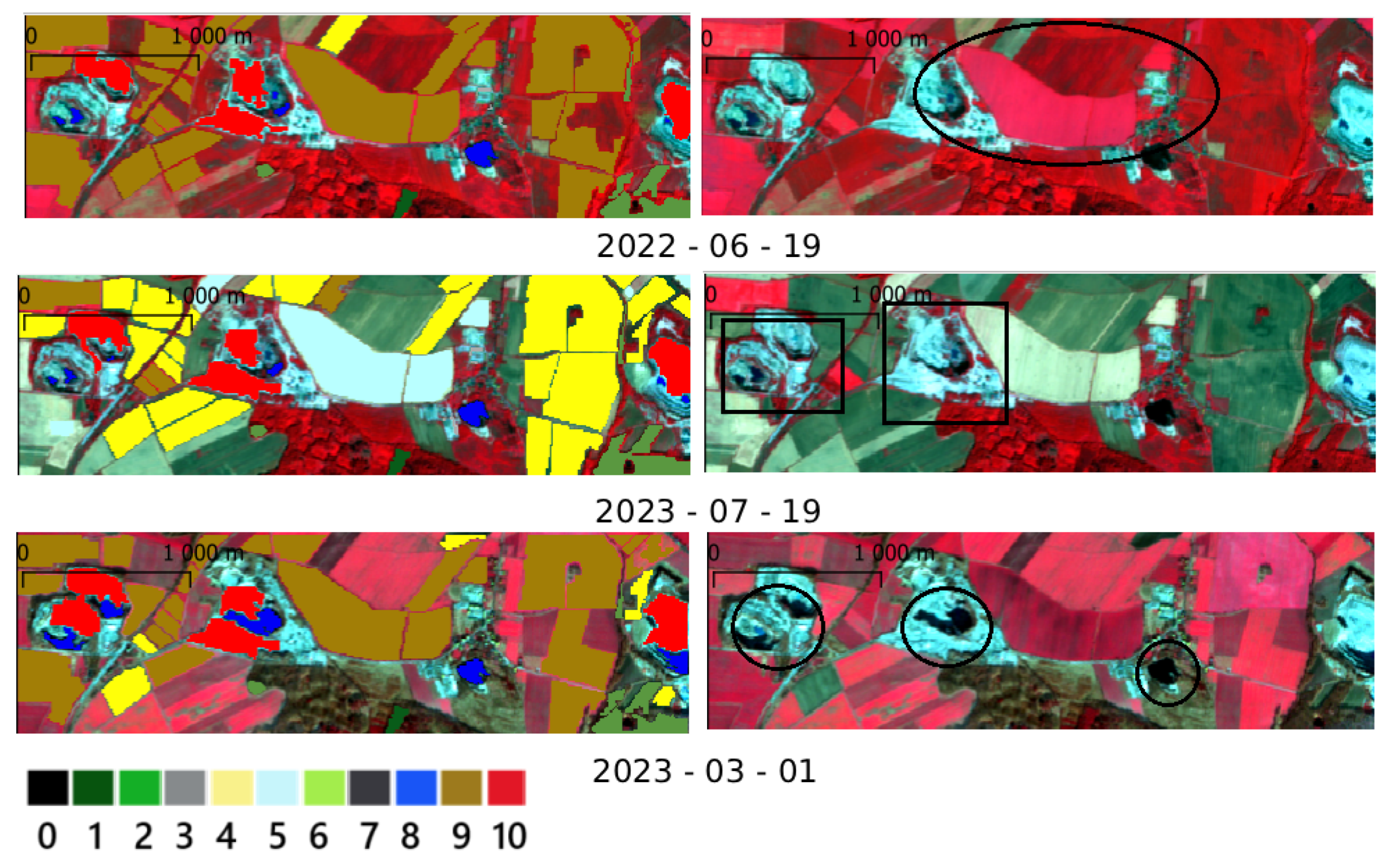
In remote sensing-based image classification, the spectral and spatial characteristics of land cover objects often vary temporally, particularly in areas dominated by vegetation—both permanent and seasonal (Figure 3). While such temporal variability is typically leveraged to improve classification accuracy in vegetation studies, it poses a substantial challenge for the consistent detection of mining features. Open-pit mines frequently exhibit spectral signatures similar to bare soil or artificial surfaces, making them difficult to distinguish using standard classification approaches. The goal of our study was to train a convolutional neural network capable of accurately detecting mining areas while concurrently performing comprehensive LULC classification. The innovative aspect of our approach was the inclusion of appropriately defined classes for agricultural vegetation, allowing for classification independent of the image acquisition date in independent regions not included in the training set.
To implement this approach, a tailored LULC classification scheme was developed. The following classes were adopted in our study:
  • Conifer forest;
  • Mix forest;
  • Urban;
  • Crops: crops before harvest or in spring before carrying out agrotechnical treatments;
  • Bare soils;
  • Permanent grassland;
  • Roads;
  • Waters;
  • Crops in vegetation stage;
  • Quarries, open pits.
Classes 4 and 9 are particularly noteworthy, with Class 9 including crops in the intensive vegetation phase, visible in red in the VNIR composition (Figure 4), and Class 4 including crops before harvest or in spring, visible in green in the VNIR composition.
It is important to note that, for the purposes of model training, the same area may receive different labels depending on the season or the state of vegetation. This is due to the spectral variability associated with different agricultural growth phases, which can affect the visual similarity between classes.
An example of interpreting a false-color composite (NIR as red, R as green, and G as blue) is shown in Figure 4. Three LULC types are compared: an agricultural field (marked by an ellipse), quarries (marked by rectangles), and water bodies (marked by circles), for three different acquisition dates. On the left, “masks” from annotated images are shown. The same agricultural field may be classified as Class 9, Class 5, and again Class 9 in spring.
In contrast, open-pit mines marked with rectangles have a characteristic cyan color and a folded texture caused by the layered excavation of the deposit, and are always annotated as Class 10. Water may also be present within the open pit, with a varying surface area (note the different extent of Class 8 annotations inside the quarry), unlike other water bodies whose surface area remains relatively constant.
This variability is a critical consideration for effective model training and enables classification that is independent of image acquisition date, which presents a unique challenge compared to traditional ML approaches.
This approach requires careful selection of training samples that represent different states of the same area (e.g., spring, summer, autumn). With appropriate training, the model can effectively distinguish these variations, allowing accurate classification of both mining areas and agricultural lands regardless of seasonal or environmental changes.

2.3. Comparison of Deep Learning and GEE-Based Classification Methods

This study explores and compares two fundamentally different approaches to land use and land cover (LULC) classification in mining-affected regions: (1) a deep learning-based semantic segmentation model (U-Net) and (2) classical supervised classification algorithms implemented in Google Earth Engine (GEE), namely CART, Random Forest, and Support Vector Machine.
While both approaches utilize Sentinel-2 imagery as input, they differ significantly in terms of data requirements, spatial generalization capabilities, and model structure. The U-Net model was trained on spatially diverse samples from three regions (Strzegom, Kolbuszowa, Kraków), enabling it to generalize across varying land cover types. In contrast, the GEE-based classifiers were trained and tested solely on data from Strzegom, focusing on pixel-level classification within a single region.
This methodological comparison provides insights into the strengths and limitations of each approach, especially in detecting spectrally ambiguous classes such as bare soil and open-pit quarries. The results highlight the advantages of deep learning in complex, heterogeneous landscapes, while also evaluating the practical value of lightweight, easily deployable models within GEE.

2.3.1. U-Net Model Training and Evaluation

The choice of the network architecture was influenced by several factors. Satellite imagery used in the project was selected and prepared specifically for Polish conditions, ensuring that the results align with the needs of governmental agencies. This also allows for the creation of a local labeled database that can support long-term monitoring. Since all training data were generated internally, it was important to adopt an architecture that can generalize well from relatively limited datasets. Another key requirement was that the model could be trained and fine-tuned on computers with average technical specifications, equipped with mid-range graphics cards commonly available in public institutions. Flexibility in defining and adapting the model in PyTorch 1.13.0 was also essential.
Before selecting the final architecture, several alternatives were analyzed and tested in simplified pilot experiments:
  • U-Net++: Expected to improve classification accuracy but with substantially higher computational requirements;
  • FCN: A lighter architecture with lower computational load, but potentially weaker performance in delineating small or irregular features;
  • U-Net: Selected as the most suitable compromise between accuracy, efficiency, and ease of implementation.
Although recent research has shown promising results with self-attention and Transformer-based models (e.g., Pixel-Set Encoders, dual-attention CNNs, FCIHMRT), these approaches typically demand larger annotated datasets and high-end computational resources. For our application, the priority was to design a workflow that could be easily adopted in operational contexts with limited resources. For this reason, we deliberately adopted the U-Net architecture integrated with Google Earth Engine classifiers. U-Net provides robust performance on moderate datasets, generalizes across different regions and seasons, and can be efficiently deployed on widely accessible hardware.
A custom U-Net implementation Figure 5 was created in PyTorch 1.13.0, inspired by the original architecture described in [25].
Table 4 summarizes the differences between the original U-Net and our implementation. In addition to the core design, our implementation facilitates reproducibility and scalability by enabling straightforward adaptation to new datasets and seamless integration with geospatial workflows.
The research was carried out in 2021 on a mid-range gaming laptop Lenovo Legion Y540 manufactured by Lenovo Group Limited (Beijng, China), equipped with an Intel i7-9750H processor (12 cores, 4.5 GHz), an NVIDIA GeForce GTX 1660 Ti Mobile graphics card, and the Linux (Debian) operating system.
The main differences between original U-Net [25] and the proposed model are as follows:
  • Increased number of convolutions from 2 to 3.
  • Added BatchNorm2d (Batch Normalization).
  • Use of padding = same.
  • Added ReplicationPad2d in the decoder before concatenation.
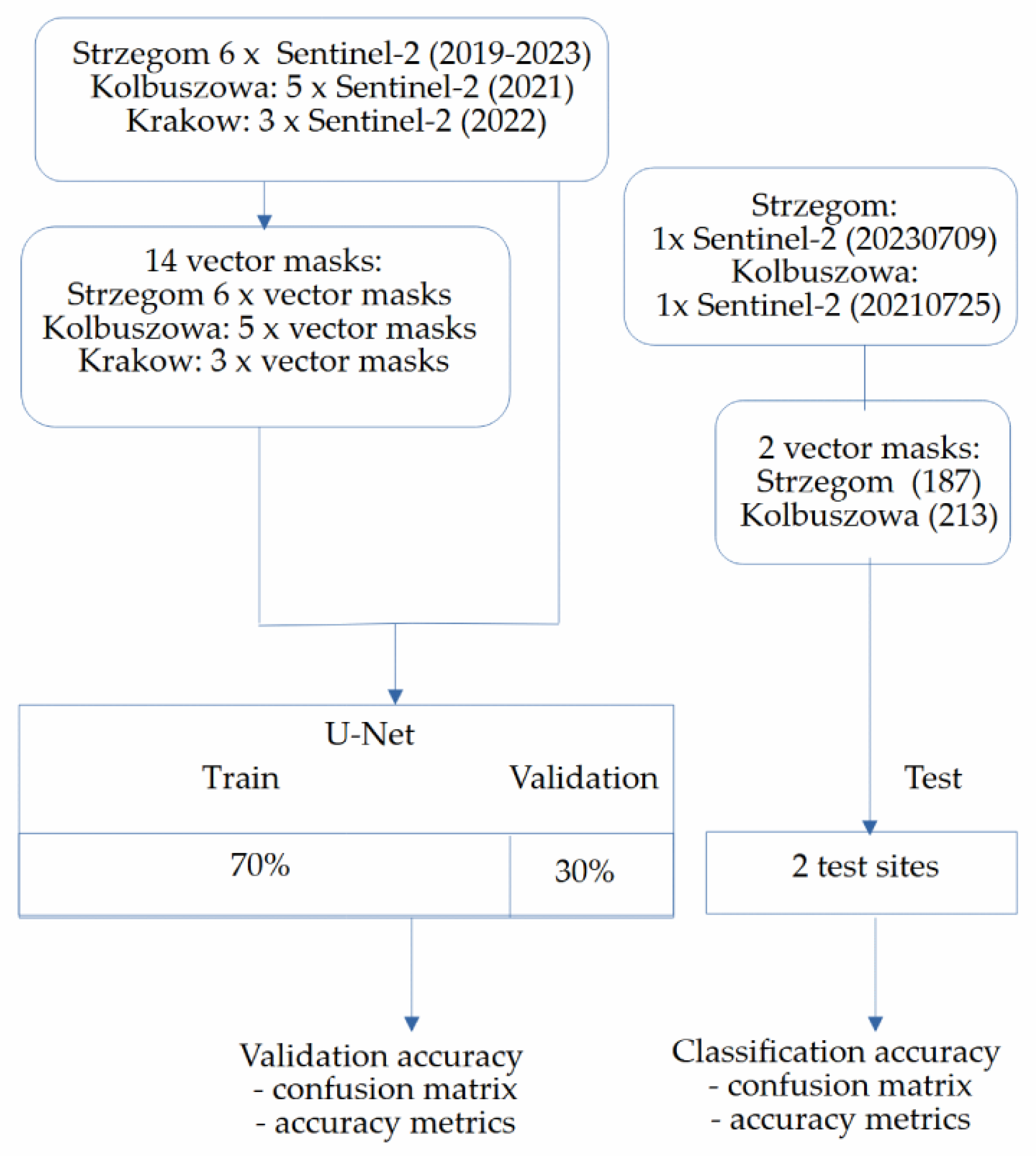
The data processing workflow in our U-Net based proposed model is presented in Figure 6. The dataset used in the present investigation was previously used in the project reported in [41].
  • Training and validation:
    • Strzegom: 20210619, 20220619, 20220719, 20221012, 20230209, 20230301;
    • Kolbuszowa: 20210327, 20210411, 20210509, 20210728, 20210906;
    • Krakow: 20220603, 20220603, 20220603.
  • Testing:
    • Strzegom: 20230709;
    • Kolbuszowa: 20210725.
For the classification, we used the above Sentinel-2 images (10 bands, excluding B1 and B10). All bands were resampled to a spatial resolution of 10 m, either natively (for B2–B4, B8) or using bilinear interpolation for bands originally provided at a resolution of 20 m (B5–B7, B8A, B11–B12). This harmonization enabled pixel-wise classification using a unified spatial grid.
The U-Net architecture [25] is a convolutional neural network widely used in remote sensing for semantic segmentation. It consists of an encoder (contracting path) that extracts features and a decoder (expanding path) that restores spatial resolution, enhanced by skip connections.
During training, Sentinel-2 image patches with a maximum size of 500 × 500 pixels and up to 10 bands were used as input. Each input patch was accompanied by a corresponding manually annotated vector mask representing one of ten land cover classes: (1) coniferous forest, (2) mixed forest, (3) urban areas, (4) agricultural crops before harvest or in spring before carrying out agrotechnical treatments, (5) bare soils, (6) permanent grassland, (7) roads, (8) water bodies, (9) crops in vegetation stage, and (10) open-pit quarries.
Training samples were sourced from three diverse regions—Strzegom, Kolbuszowa, and Kraków—spanning different years (2019–2023). A total of 14 annotated vector masks (6 from Strzegom, 5 from Kolbuszowa, and 3 from Kraków) were used to build the training and validation datasets. The dataset was randomly split using a 70/30 ratio for training and validation, respectively. Additionally, two held-out test scenes (Strzegom 2023-07-09 and Kolbuszowa 2021-07-25) were used for independent testing, each accompanied by a corresponding reference mask.
We first scoped reasonable ranges for the training setup and then ran targeted experiments within those bounds. In this context, “parameters” refers to all variables affecting training, from patch_size to hyperparameters (e.g., learning rate, weight decay). The configuration used for the main runs is summarized in Table 5.
Preliminary experiments were conducted to establish suitable parameter ranges, followed by detailed tests using selected values from these ranges. Here, the term parameters refers to all variables affecting the training process, from patch_size to network hyperparameters such as learning rate and weight decay. An example configuration of script arguments, including the tested hyperparameter weight_decay, is presented in Table 5.
The tensorboard tool was used to monitor and log the training process. Example tensorboard logs are shown in Figure 7.
An example loss function plot when testing various values of two hyperparameters, learning rate and weight decay, with the CrossEntropyLoss loss function is shown in Figure 8.
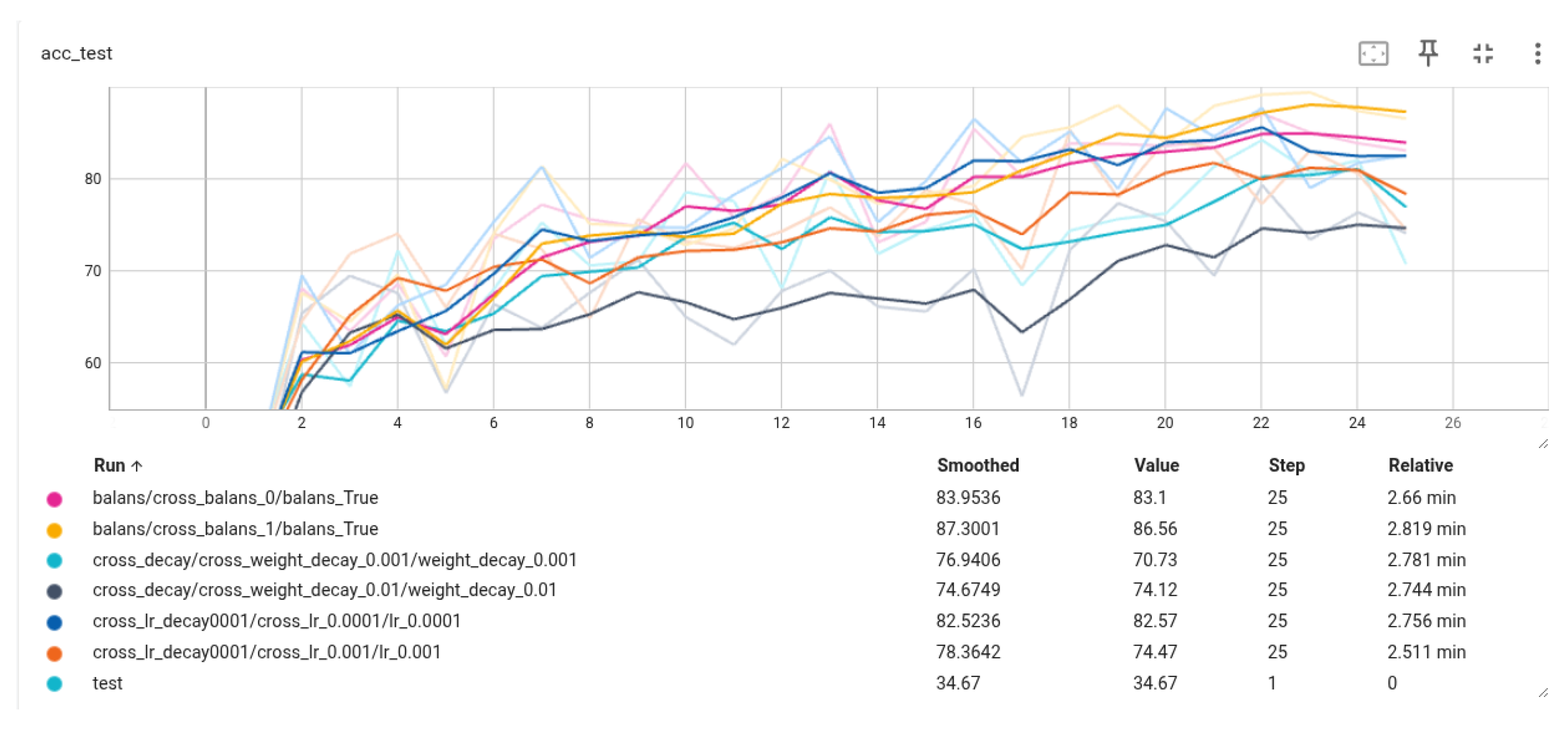
Figure 9 presents an example accuracy plot when testing the following:
  • The use or non-use of class weights (class balancing).
  • Various values of two hyperparameters: learning rate and weight decay with the CrossEntropyLoss loss function.
Accuracy metrics were computed on both validation data and independent test sites. Validation was used to optimize the model parameters and detect overfitting, while the final classification performance was assessed in unseen regions. The metrics included Overall Accuracy, class-wise accuracy, and confusion matrices.
All relevant data used in U-Net classification—including satellite imagery, annotated reference masks, classification results, and accuracy evaluation—are available in the project repository: U-Net dataset repository (https://github.com/bh-del/lulc_mining, accessed on 24 August 2025).

2.3.2. Supervised Classification in Google Earth Engine

The purpose of the U-Net classification comparison was to use the GEE tools in a standard manner, without any special preprocessing of satellite data. Therefore, a single Sentinel-2 image was used instead of a multi-temporal collection, which is indeed possible to apply in GEE but requires more advanced knowledge and preparatory steps (example script) (https://code.earthengine.google.com/37b32c3ac33df997080482ee862e4ce3) [accessed on 29 July 2025].
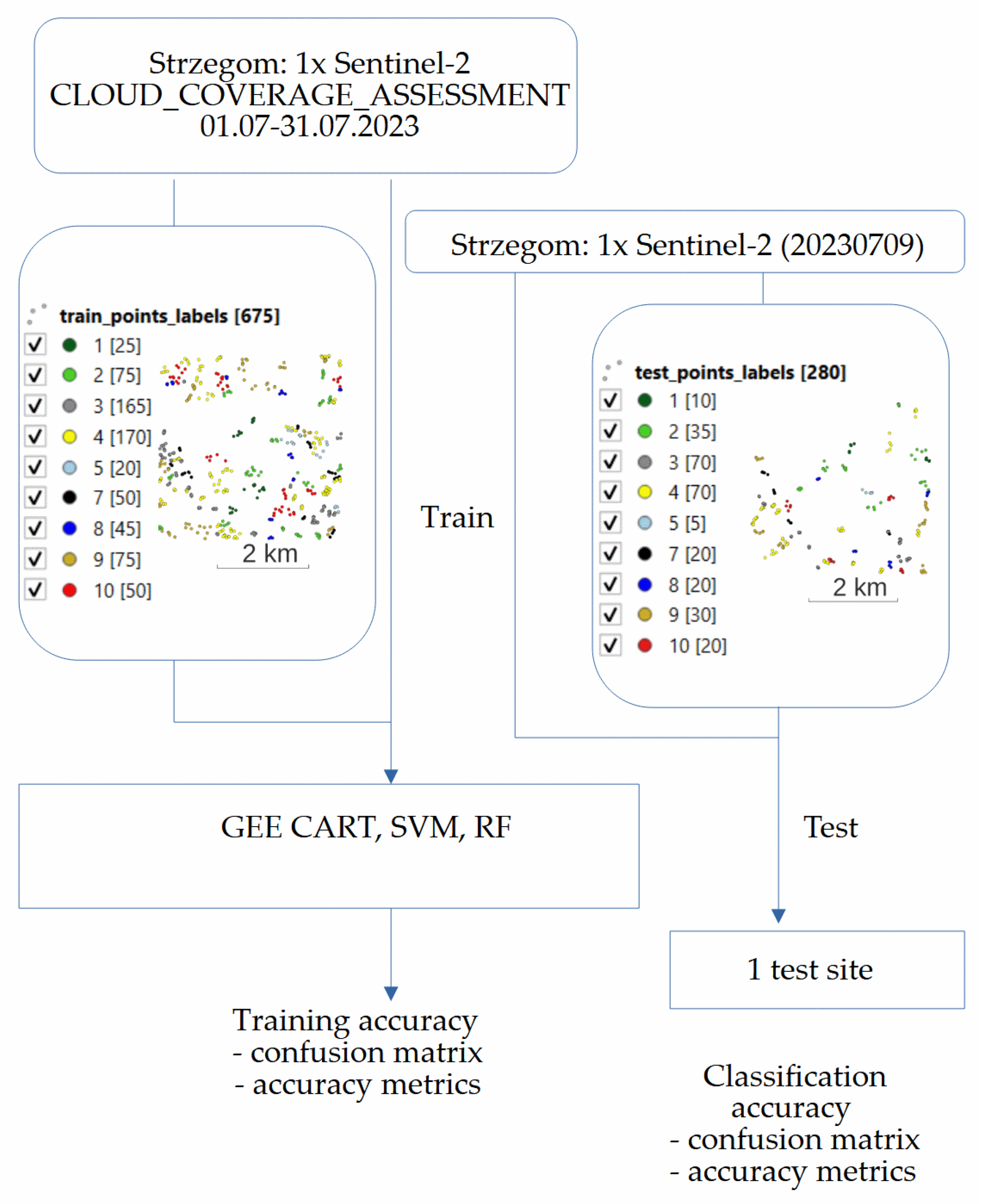
The data processing workflow is presented in Figure 10. In contrast to the deep learning approach, the GEE-based classification was conducted using data from a single area—Strzegom. The reference vector data were manually vectorized and automatically divided into training (70%) and testing subsets (30%) (675 training points and 280 test points).
In this study, we used Sentinel-2 Level-2A surface reflectance imagery available through the Harmonized Sentinel-2 MSI collection in Google Earth Engine (COPERNICUS/S2_SR_HARMONIZED). This collection includes atmospherically corrected data processed with Sen2Cor and harmonized across processing baselines to ensure consistency in DN scaling.
The dataset provides 12 spectral bands (B1–B12, excluding B10) as unsigned 16-bit integers (UINT16), representing surface reflectance scaled by a factor of 10,000. Importantly, each band retains its original spatial resolution:
  • 10 m: B2 (blue), B3 (green), B4 (red), B8 (NIR).
  • 20 m: B5, B6, B7, B8A, B11, B12.
  • 60 m: B1 and B9 (B10 is omitted in L2A).
As a result, the spatial resolution of the bands is not uniform within the dataset. Any application requiring band stacking (e.g., classification using all bands) must perform resampling or reprojection to a common resolution, typically 10 m. This step in GEE was applied automatically by the classifier, which was particularly convenient, as we aimed to use the simplest possible approach.

2.3.3. Google Earth Engine: Data Selection and Preprocessing

The data processing workflow in GEE is illustrated in Figure 10.
The scene was filtered and selected on the basis of the CLOUD_COVERAGE_ASSESSMENT metadata field provided by ESA’s Copernicus service. This metadata quantifies the estimated percentage of cloud coverage in the product, and only images with near-zero values (i.e., fully cloud-free or cloudless over the region of interest) were considered. The selection process utilized the following GEE query:
Sentinel2
  .filterDate(“2023-07-01”, “2023-07-30”)
  .filterBounds(region)
  .sort(“CLOUD_COVERAGE_ASSESSMENT”)
  .first();
Due to limitations on the size of vector files that can be uploaded to GEE, the reference dataset—originally in polygon format—was converted into a set of points, with several points placed within each polygon. The training dataset consisted of reference points: 675 points for training and validation, while the test dataset included 280 points. These prepared points were then uploaded to GEE. These reference points were then used to train and test the classification models, CART, Random Forest, and SVM, as implemented in GEE.
Three supervised machine learning algorithms were tested:
  • Classification and Regression Trees (CART)—A rule-based, non-parametric method that recursively splits the data into binary decision trees to maximize class purity [52].
  • Random Forest (RF)—An ensemble learning method that aggregates predictions from multiple decision trees trained on bootstrap samples. RF is robust to overfitting and handles high-dimensional data well [53].
  • Support Vector Machine (SVM)—A margin-based classifier that constructs an optimal hyperplane to separate classes. We used a linear kernel and C-SVM formulation [54].
The model training in Google Earth Engine (GEE) was performed using three built-in supervised classification algorithms available through the ee.Classifier module: smileCart(), smileRandomForest() and libsvm(). These functions are part of GEE’s interface to the Smile machine learning library and represent widely used, non-parametric classification techniques with varying complexity and generalization capabilities. The GEE classifiers smileCart(), smileRandomForest(), and smileSvm() are built upon the Smile library [55], which provides scalable implementations of many classical machine learning algorithms.
The smileCart() function implements Classification and Regression Trees (CART), a decision tree algorithm that partitions the feature space into axis-aligned regions based on threshold splits. CART models are simple, interpretable, and computationally efficient, making them suitable for baseline land cover classification tasks. However, they are prone to overfitting and limited in capturing complex, non-linear class boundaries.
The smileRandomForest() function constructs an ensemble of decision trees using the Random Forest algorithm. Each tree is trained on a bootstrap sample of the training data, with a random subset of features selected at each node split. The final classification is obtained via majority voting across all trees. Random Forests typically offer improved accuracy and robustness compared to single-tree models and are less sensitive to noise and overfitting.
The libsvm() function provides an interface to Support Vector Machine (SVM) classifiers. By default, GEE uses a linear kernel, which separates classes with a hyperplane that maximizes the margin between class boundaries. SVMs are effective in high-dimensional spaces and can generalize well with limited training samples, especially when class separation is relatively clean.
All classifiers were trained using the same set of spectral bands (B2–B8A, B11–B12) extracted from the Sentinel-2 scene and the same vector-based ground truth masks. The final step in the GEE classification process was the calculation of confusion matrices for the training and testing datasets.
The GEE-based classification workflow included the following steps:
  • Selecting the region of interest (Strzegom) and Sentinel-2 scene;
  • Extracting and clipping spectral bands to ROI;
  • Sampling training pixels from labeled vector data;
  • Training three classifiers: CART, RF (10 trees) and SVM (linear kernel);
  • Applying the models to classify the image;
  • Visualization of classification maps using predefined palettes;
  • Export of classified outputs;
  • Performance evaluation using accuracy metrics derived from confusion matrices.

2.4. Code and Data Availability

All code used for supervised classification in Google Earth Engine (GEE) is openly accessible at the following link:
The manually labeled training and testing datasets used in this study are available as public GEE assets:
These assets can be directly imported into any Earth Engine script for reproduction or further analysis.

2.5. Accuracy Metrics

To ensure a reliable comparison between classification approaches, the accuracy assessment was performed independently for both the deep learning model (U-Net) and the classical machine learning classifiers implemented in Google Earth Engine (GEE).
In the case of U-Net (Figure 6), the performance of the model was evaluated using a two-level approach. First, accuracy was computed on a held-out validation subset (30%) derived from the same spatial pool as the training data. Second, an independent test was performed using Sentinel-2 scenes and reference masks from two geographically distinct locations not used in model training and without using any training data from the tested locations. This setup enabled a robust assessment of both within-region generalization and transferability across space.
For GEE-based classifiers (Figure 10), accuracy was assessed at two levels: (1) on the training set (resubstitution accuracy), reflecting the model’s ability to fit the labeled samples, and (2) on an independent test set composed of manually labeled validation points, allowing evaluation of generalization performance under operational conditions.
Performance evaluation relied on standard classification metrics derived from confusion matrices, which remain the foundational tool for accuracy assessment in both remote sensing and machine learning contexts [56]. In both approaches (U-Net and GEE), confusion matrices and aggregate accuracy measures served as key indicators of classification performance.
Evaluating the performance of classification models requires the use of standardized metrics derived from the confusion matrix, a fundamental tool that tabulates true and false predictions. Table 6 summarizes the most commonly used accuracy metrics, including overall and class-specific measures.
  • Accuracy (ACC) quantifies the proportion of correctly predicted instances on the total number of samples.
  • Specificity (TNR) measures the ability to correctly identify negative cases.
  • Overall Accuracy (OA) represents the proportion of all correctly classified pixels (i.e., the sum of all true positives) in the total sample size.
  • Producer Accuracy (PA), also known as recall or sensitivity, reflects the ability to correctly classify a given class.
  • User Accuracy (UA), or precision, indicates how many of the predicted instances of a class are correct.
  • F1-score is the harmonic mean of precision and recall, providing a balanced measure for uneven class distributions.
The definitions of the main evaluation metrics used in this study are provided in Table 6.
Due to the confusion surrounding the interpretation of accuracy metrics, the following two subsections include a brief computational example to clarify this issue.

2.5.1. Binary Classification Case Study

Table 7 presents a confusion matrix for a binary classification example. The metrics derived in Table 8 show an Overall Accuracy (ACC and OA) of 0.85, a recall of 0.80, and a precision of 0.89, leading to an F1-score of approximately 0.84. These metrics highlight a relatively balanced classification with moderate class separation.

2.5.2. Multiclass Classification Case Study

To assess model performance on multiple classes, a 3-class confusion matrix is shown in Table 9. The matrix is decomposed into per-class confusion components (Table 10) and corresponding class-wise metrics (Table 11). These one-vs-all evaluations reveal varying accuracy levels across classes, particularly lower precision for class C (0.595), indicating frequent misclassifications.

2.5.3. Macro-Averaged Metrics

Table 12 presents macro-averaged values across all classes. It is worth noting the substantial discrepancy of approximately 10 percentage points between accuracy (ACC = 0.818) and Overall Accuracy (OA = 0.724). Moreover, the metrics commonly used in machine learning, such as ACC and specificity (TNR = 0.866), appear significantly high. In contrast, the metrics traditionally favored in remote sensing—including PA, UA, and F1-score—are mutually consistent and align closely with OA.
This example alone raises concerns about potential overestimation of classification performance when relying solely on ACC or TNR, especially when macro-averaged ACC is misleadingly reported as OA. Such practices may inflate perceived accuracy and obscure weaknesses in class-specific predictions. As shown by Foody [56], careful interpretation of these indices is critical in both remote sensing and machine learning contexts.

3. Results

3.1. Classification Using the Trained U-Net Network

An accurate assessment was conducted in two areas. The trained U-Net model was used to classify two Sentinel-2 images acquired on dates different from those used for training. Training fields were not included in the classification process. The confusion matrix was calculated on the basis of manually digitized polygons, which were visually interpreted directly from the satellite image.
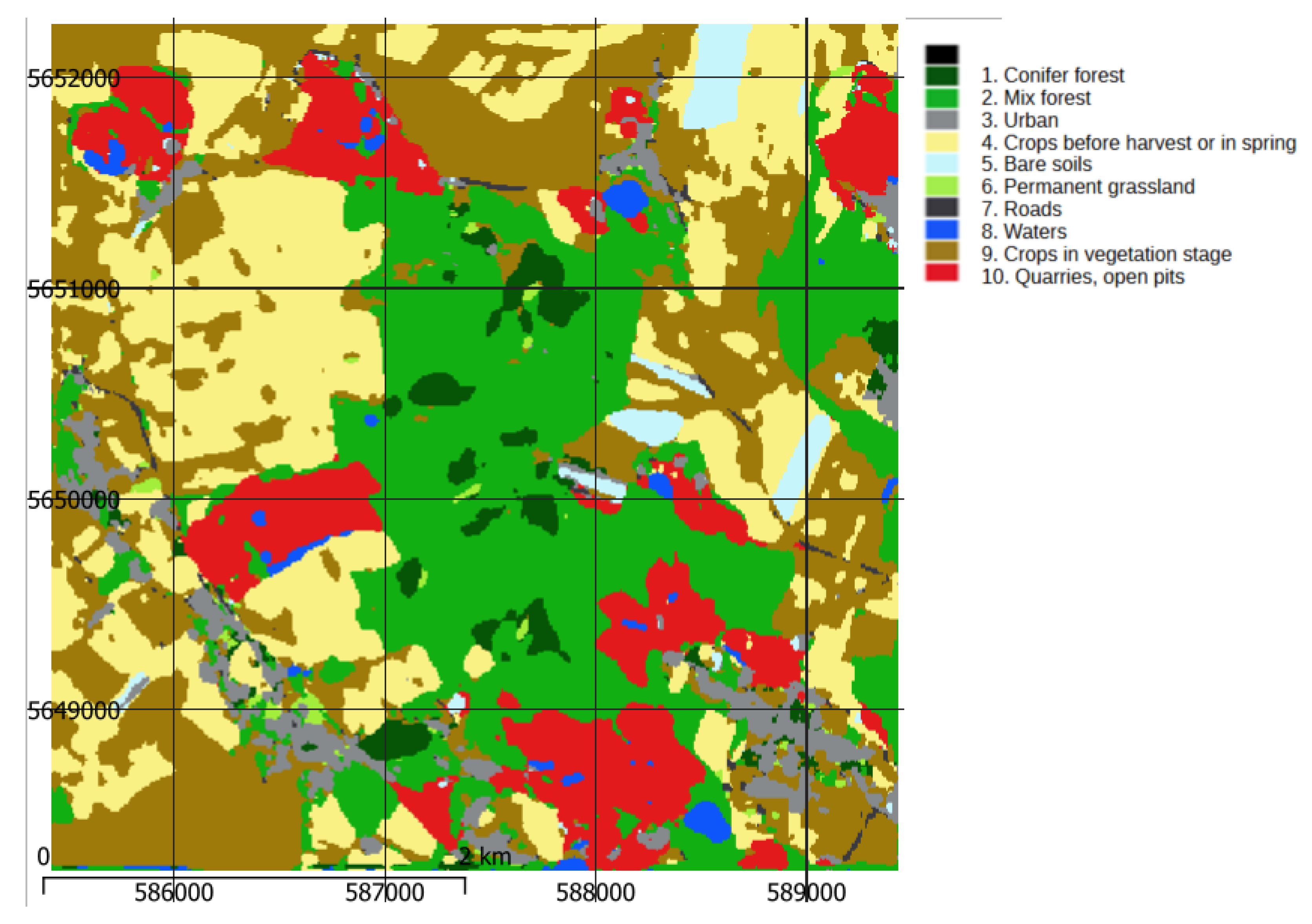
The performance of the U-Net classifier was evaluated using independent test datasets, and the results are summarized in terms of confusion matrices (Table 13 and Table 14) and standard accuracy metrics (Table 15 and Table 16). Visual examples of the classification results are shown in Figure 11 and Figure 12.
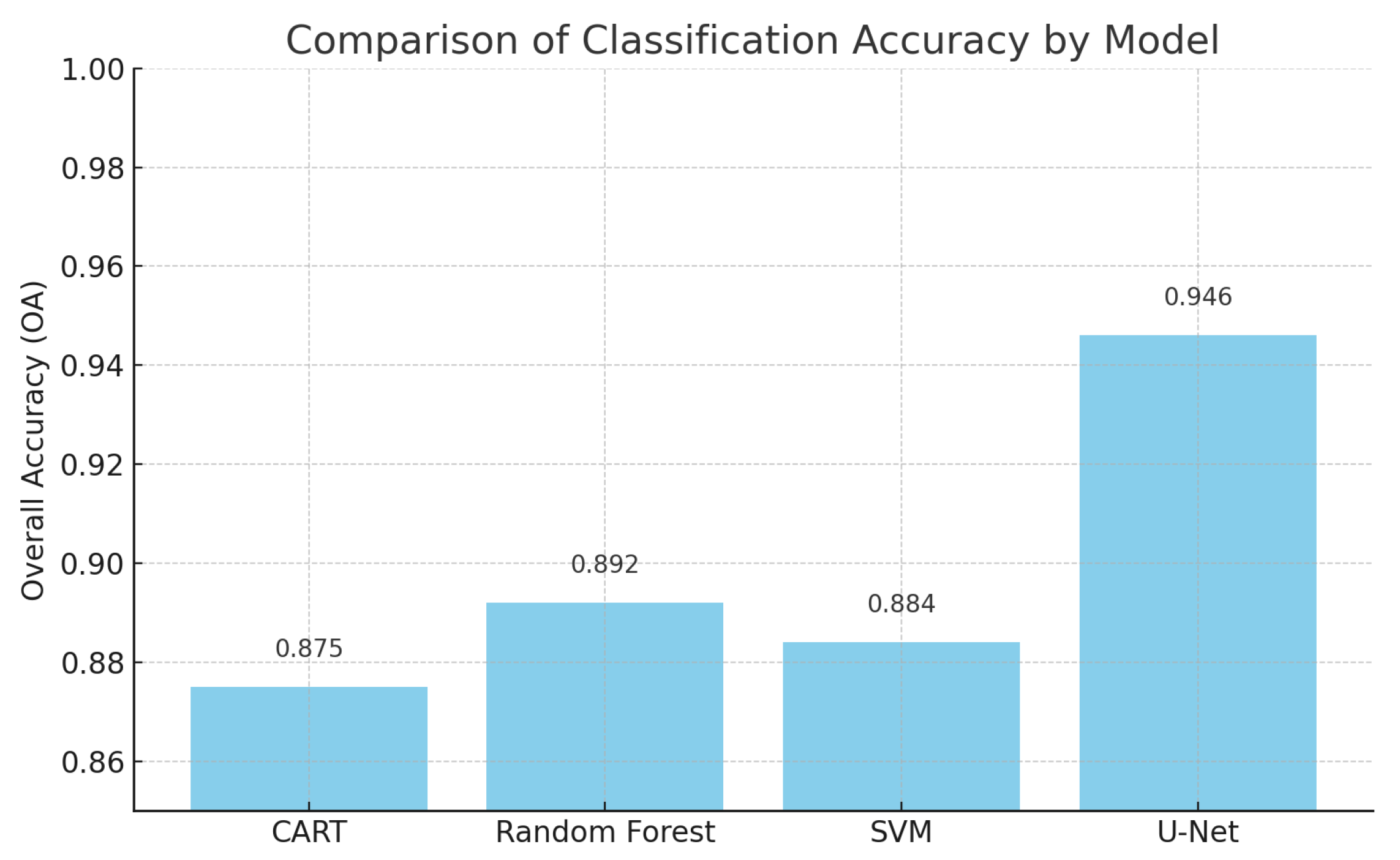
For the Strzegom site, the U-Net achieved an Overall Accuracy (OA) of 94.60%, while for Kolbuszowa, the OA reached 93.11%. These results demonstrate the strong generalization capability of the model in both anthropogenic and natural landscapes.
The per-class accuracy metrics further highlight the effectiveness of the classifier. In Strzegom, the average class-wise accuracy (ACC) was 98.81%, with an average Producer’s Accuracy (PA) of 92.07%, User’s Accuracy (UA) of 84.04%, and F1-score of 87.07%. Similarly, in Kolbuszowa, the mean ACC was 98.47%, with PA at 90.30%, UA at 88.63% and F1-score at 89.02%.
The highest performance was observed in classes with distinctive spectral signatures, such as Class 8 (water) and Class 10 (quarries, open pits), both achieving F1-scores exceeding 0.96. On the other hand, Class 7 (roads) exhibited the lowest performance in both study areas (mainly due to Sentinel-2’s spatial resolution—10 m), with a notably low UA (36.88% in Strzegom and 53.57% in Kolbuszowa), indicating frequent confusion with spectrally similar categories.
These results suggest that the U-Net model is robust and adaptable to varying land cover typologies. Its strength lies particularly in detecting well-defined structures and land cover with clear spectral and spatial patterns. However, further refinement—such as incorporating auxiliary data or class aggregation—may be necessary to improve the classification accuracy for mixed or ambiguous classes.
For benchmarking purposes, a comparative evaluation using the CART, Random Forest (RF), and Support Vector Machine (SVM) classifiers implemented in Google Earth Engine was performed exclusively for the Strzegom area. The results of this comparison, including quantitative metrics and qualitative differences, are presented and discussed in the following subsection.

3.2. Classification Using GEE: CART, RF and SVM

The performance of machine learning classifiers implemented in Google Earth Engine (GEE)—CART, Random Forest (RF), and Support Vector Machine (SVM)—was evaluated for the Strzegom region using the same metrics as for U-Net. Table 17 provides a summary of Overall Accuracy (OA), Producer’s Accuracy (PA), User’s Accuracy (UA), and F1-score for each model, with class-wise metrics presented in detail in Table 18, Table 19 and Table 20.
Among the GEE-based classifiers, Random Forest (RF) achieved the highest Overall Accuracy (OA) of 80.00%, slightly outperforming SVM (78.57%) and CART (76.79%). However, the strengths of each method varied depending on the class.
It is also important to highlight the discrepancy between the average class accuracy (ACC) and Overall Accuracy (OA), which is particularly evident in the CART classification. Reporting the average ACC value of 94.84% as the accuracy metric may give a misleading impression of high classification performance, while the actual OA is only 76.79%. In fact, the average ACC values for all GEE-based methods are approximately 95%, further emphasizing the need for careful interpretation of accuracy metrics.
  • CART showed balanced performance across classes, with average PA, UA, and F1-score values close to 0.77. Its robustness in identifying less represented classes (e.g., Class 5 and Class 10) was notable.
  • RF, while delivering the best OA, exhibited lower recall (PA = 0.7098), indicating a tendency to miss some true class instances, despite strong precision (UA = 0.7295).
  • SVM demonstrated better recall (PA = 0.7421) than RF, but with slightly lower overall precision (UA = 0.7385). F1-scores for SVM were overall higher than CART, showing its strength in classifying well-defined land cover types.
Despite the acceptable performance of the GEE classifiers, particularly in classes like water (Class 8) and open quarries (Class 10), all three models showed limitations in detecting narrow or mixed land covers such as roads (Class 7), which exhibited F1-scores below 0.60 across the board.

3.3. Comparison of U-Net and GEE-Based Classification Approaches

In contrast, the deep learning model based on the U-Net architecture consistently outperformed the GEE-based classifiers in both study areas.
For the Strzegom site, U-Net achieved the following:
  • Overall Accuracy (OA): 94.60%.
  • Mean PA: 92.07%.
  • Mean UA: 84.04%.
  • Mean F1-score: 87.07%.
This represents a 13–18 percentage point increase in OA compared to GEE models and even higher gains in recall and precision per class.
U-Net demonstrated excellent generalization across heterogeneous landscapes, especially for spectrally distinct classes such as water and quarries, which achieved F1-scores above 0.96. Even challenging classes such as roads showed improved recall (PA = 70.24%), although precision remained relatively low (UA = 36.88%), mainly due to the spatial resolution limits of Sentinel-2 imagery.
These results underscore the advantage of deep learning models in capturing spatial context and complex class boundaries, making U-Net particularly suitable for fine-grained land cover mapping. Although GEE classifiers provide fast and interpretable baselines, their performance is limited by their reliance on pixel-based decision rules. Deep convolutional networks such as U-Net can effectively leverage both spectral and spatial information, leading to more accurate and consistent results.
The comparison presented in Table 21 highlights the fundamental differences between U-Net and GEE-based classification approaches. The U-Net model, trained on multi-regional data, demonstrated strong generalization capabilities and high segmentation accuracy, making it well-suited for complex and heterogeneous landscapes. In contrast, the classifiers implemented in GEE were limited to a single region (Strzegom) and showed relatively lower precision in distinguishing spectrally similar classes, such as bare soils and open-pit areas.
From an operational perspective, GEE offers significant advantages in terms of accessibility and simplicity of implementation, since it does not require specialized hardware. However, its reliance on classical models makes it less adaptable to spatial variability and seasonal dynamics. In contrast, deep learning approaches like U-Net are computationally intensive, but provide superior performance when sufficient training data and computational resources are available.
These findings suggest that the choice of classification approach should take into account both the complexity of the study area and the available infrastructure. For regional-scale applications or policy monitoring, deep learning may provide the necessary accuracy, while GEE classifiers remain valuable for rapid prototyping and localized assessments.

4. Discussion

4.1. Effectiveness of LULC Classification for the Detection of Open Pits

The results of this study demonstrate the effectiveness of applying supervised classification algorithms to detect land use and land cover (LULC) types, with particular emphasis on open-pit mining. Using Sentinel-2 data and tailored class definitions, it was possible to identify exploitation areas with high precision, despite their spectral similarity to natural or anthropogenic surfaces such as bare soil, roads, or construction zones.
The use of a dedicated class for mining activity, along with seasonally adjusted vegetation classes (e.g., crops before and during the vegetation period), allowed for improved segmentation and classification accuracy. Specifically, the introduction of Class 4 (crops before harvest or in spring before agrotechnical treatments) and Class 9 (crops in the vegetation stage) helped differentiate vegetation phases, while separating Class 5 (bare soil) from Class 10 (quarries and pits) minimized misclassification between natural and anthropogenic bare surfaces. This was especially critical in areas such as Strzegom, where mining operations are spatially fragmented and spectrally ambiguous.
Among the algorithms tested, the deep learning U-Net model achieved the highest classification accuracy (OA = 94.6%). Its encoder–decoder structure with skip connections enables effective spatial generalization and detail preservation, which are crucial in segmenting irregularly shaped mining areas. Although traditional machine learning methods such as Random Forest and SVM also performed reasonably well, their accuracy was consistently lower and more sensitive to intra-class variability.
In the Kolbuszowa region, which is characterized by a more homogeneous agricultural landscape, U-Net maintained high performance (OA = 93.11%), with slightly lower F1-scores for classes with temporal or spectral variability, such as transitional vegetation or roads. However, its generalization capability remained strong in both natural and anthropogenic land covers.
Another important aspect highlighted in this study is the need for context-specific accuracy metrics. Although Overall Accuracy (OA) provides a general sense of performance, User Accuracy (UA) and Producer Accuracy (PA) are more informative when assessing specific land cover classes, particularly those prone to misclassification. For instance, roads (Class 7) were consistently misclassified by all GEE-based models, while U-Net, despite low precision (UA = 36.88%), showed improved recall (PA = 70.24%), capturing more true positives in narrow and elongated structures.
Importantly, class-wise accuracy (ACC) should not be confused with Overall Accuracy (OA). Although the mean ACC values are always higher (the lower the OA value, the greater the discrepancy), OA remains the only unbiased measure of total classification performance across the extent of the image.
The confusion matrices presented for each site and the classification method further revealed these class-specific weaknesses and highlighted the importance of evaluating per class rather than relying solely on aggregate measures.
In the Strzegom case study, several notable inter-class confusions were observed Table 13. Class 9 (crops in vegetation stage) was sometimes misclassified as Class 4 (crops before harvest) and Class 2 (mixed forest). The confusion between Classes 9 and 4 can be attributed to spectral similarity in late summer, when some crop fields exhibit reduced chlorophyll content and canopy density, producing reflectance patterns similar to pre-harvest conditions. The misclassification between Class 9 and Class 2 probably results from mixed pixels at the interface of cropland and forested areas, especially in fragmented agricultural landscapes. Furthermore, Class 4 occasionally overlapped with Class 2, which can occur when young forest regrowth or agroforestry plots share spectral characteristics with certain crop types during specific phenological stages. These cases underscore the need for incorporating additional temporal or ancillary data to better separate phenologically or spectrally similar classes.
Despite the superior accuracy of U-Net, several challenges remain. The 10 m spatial resolution of Sentinel-2 limits the accurate mapping of narrow or mixed land cover types, such as roads or hedgerows. Furthermore, the quality and granularity of the reference data strongly influence the performance of the model. Future work could explore the integration of auxiliary data (e.g., elevation, cadastral boundaries) or the use of higher-resolution imagery to refine model output.
The lack of a dedicated class for mining areas in most public LULC benchmarks limits the direct applicability of existing datasets for the detection of illegal activity. This underscores the importance of developing localized reference datasets or modifying existing label taxonomies to better reflect the dynamics of land cover in the real world.
Deep learning models such as U-Net have demonstrated superior performance in remote sensing classification tasks [25,57]. Their strength lies in leveraging both spatial and spectral contexts, allowing for more nuanced and consistent predictions. However, classical algorithms such as Random Forest and SVM remain valuable due to their simplicity, lower computational requirements, and interpretability [58,59]. For example, Random Forests provide direct measures of feature importance, which can aid in understanding the decision process—an aspect often lacking in deep learning approaches.

4.2. Analysis of Detected Areas for Potential Illegal Exploitation

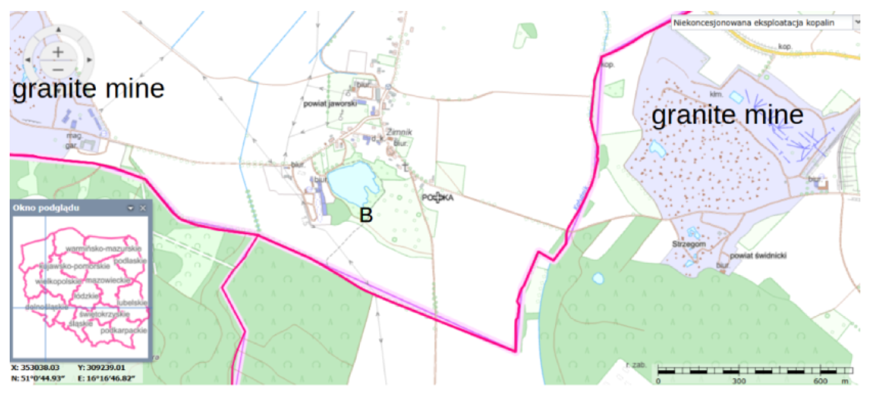
In Poland, the Open-pit Mineral Exploitation Monitoring Program (MOEK) is conducted by Polish Geological Institute (https://geoportal.pgi.gov.pl/portal/page/portal/PIGMainExtranet, accessed on 24 August 2025). The MOEK geoportal (https://emgsp.pgi.gov.pl/emgsp/, accessed on 24 August 2025) provides information on various aspects of open-pit mining, including the location of mining sites operated without a valid license. Among the published data are the coordinates of confirmed illegal extraction sites, marked as red diamonds on the MOEK maps (Figure 13). In addition, the Polish Geological Institute (PGI) operates the System of Management and Protection of Mineral Resources in Poland MIDAS (https://midas-app.pgi.gov.pl/ords/r/public/midas/mapa, accessed on 24 August 2025). To illustrate the phenomenon of illegal exploitation, which is monitored and visualized in the MOEK geoportal, a location was selected near the Strzegom test area (Figure 13, Figure 14 and Figure 15).
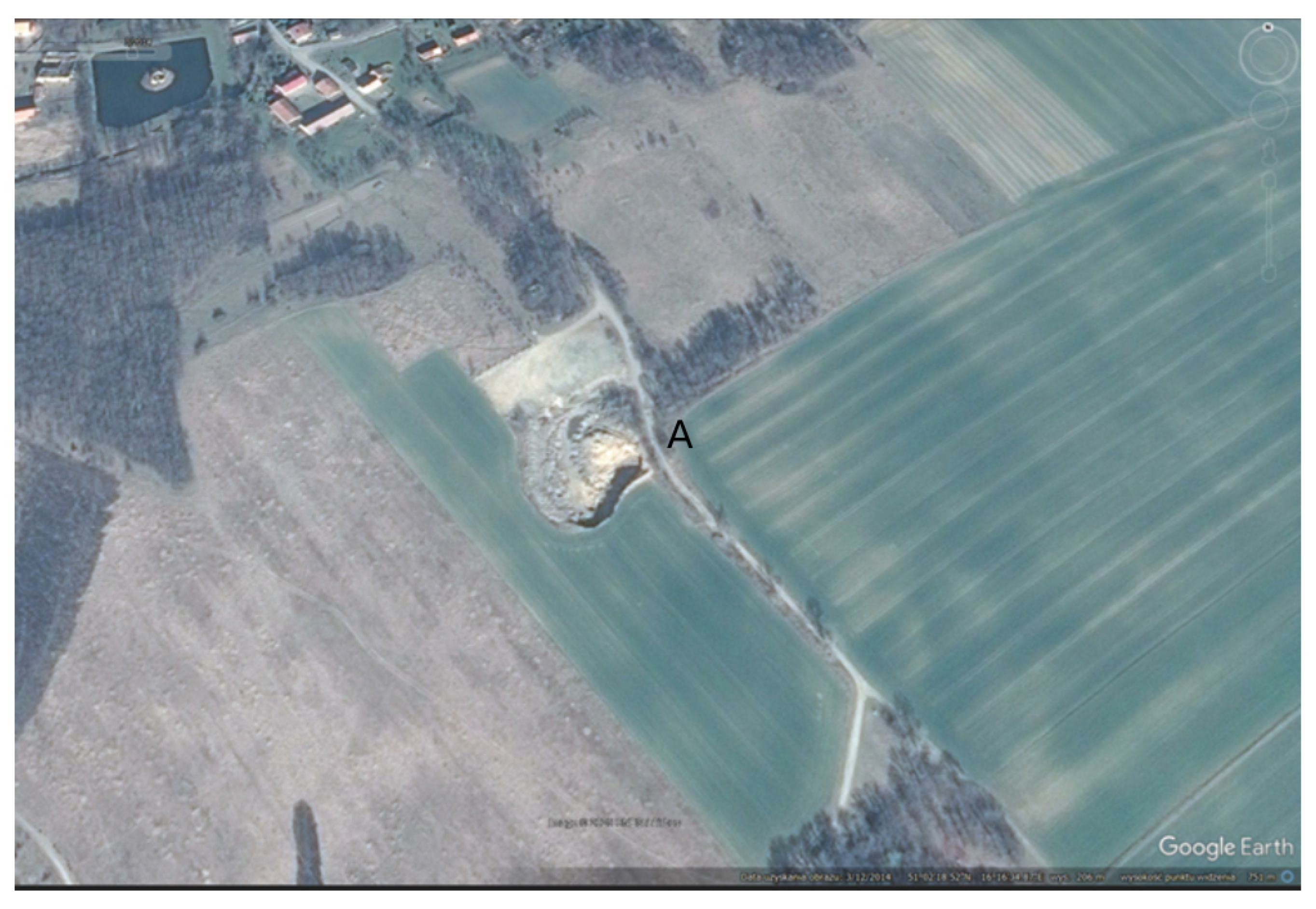
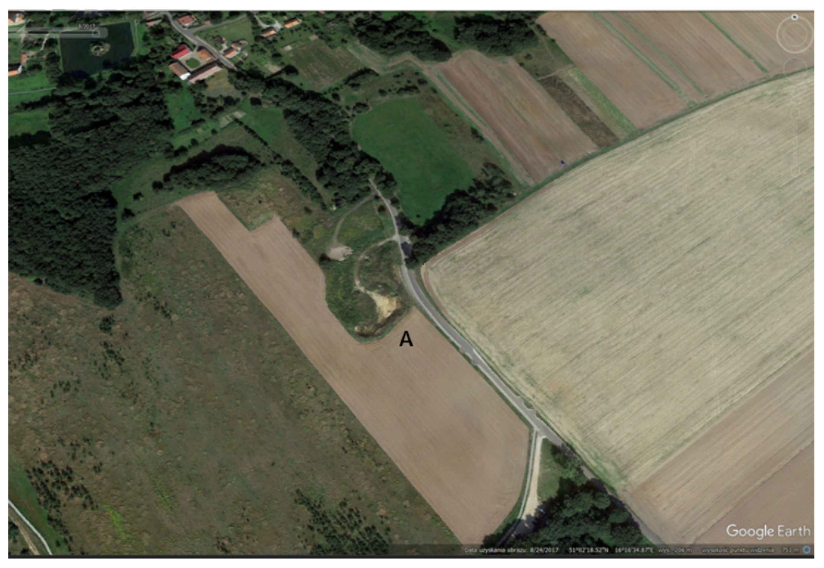
The first example is a case where small-scale illegal extraction of gravel and sand was carried out, with limited volume and spatial extent, and was not located within the area of documented mineral deposits in MIDAS. This exploitation was discontinued in 2020. The activity was carried out in an agricultural area (CORINE code 211: non-irrigated arable land). The comparison of aerial photographs confirms both the occurrence of exploitation and its cessation (Figure 16 and Figure 17).
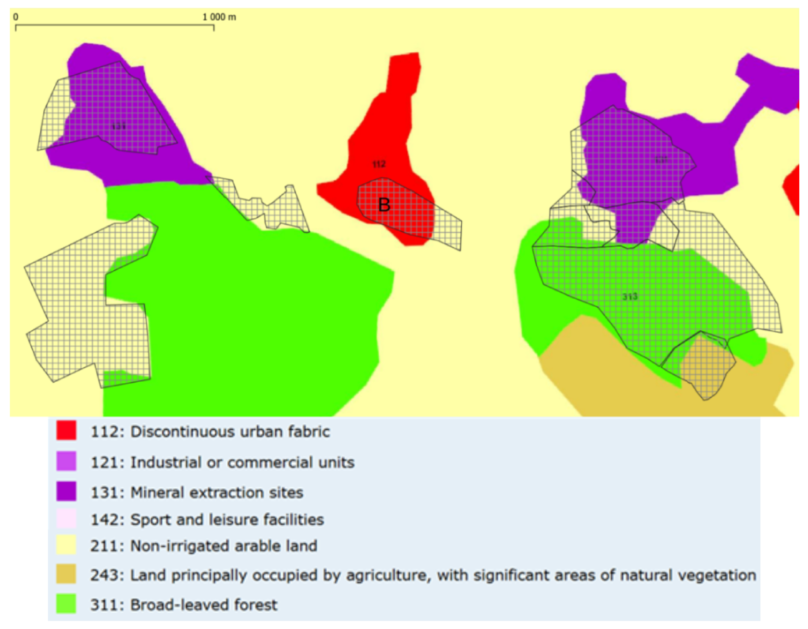
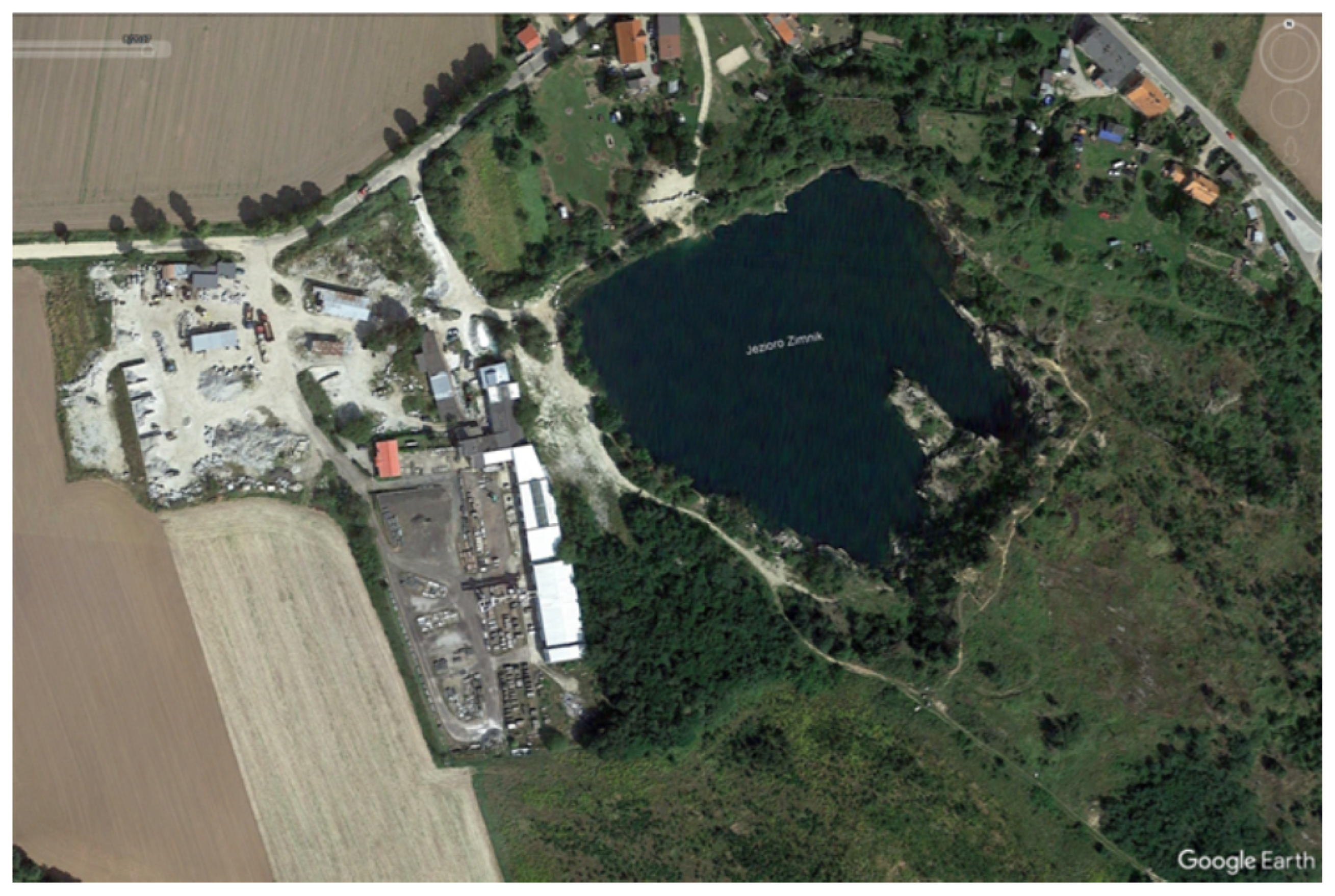
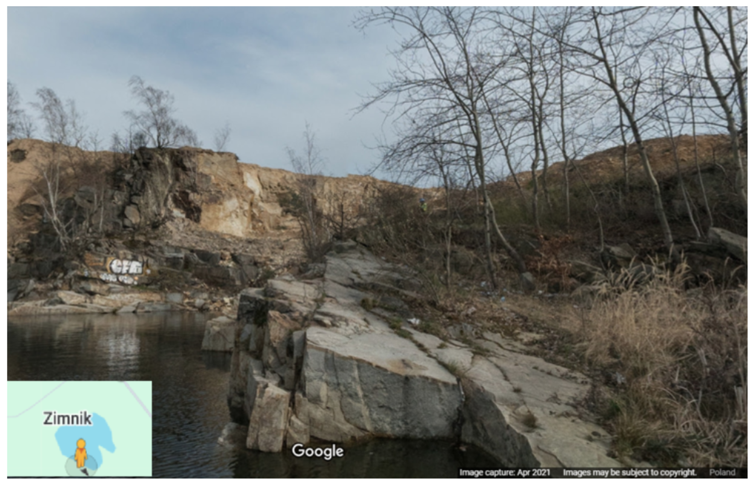
The second example (B) is located within our study area, but differs from the first example (A). Probable illegal exploitation was identified based on the Sentinel-2 image classification and was not detected within the MOEK monitoring program but located within the area of documented mineral deposits in MIDAS. The classification result for the Strzegom test area is shown in Figure 14, along with the locations of geologically recognized deposits (both exploited and unexploited), marked as hatched polygons. Case B, located outside of officially licensed mining areas (Figure 18), also exhibits the characteristics of illegal exploitation (compare also with CORINE Figure 19). The Unet classification result is in the Figure 20. Aerial images from 2017 and 2018 reveal morphological changes consistent with material extraction (Figure 21 and Figure 22). An in situ photograph from Google Maps provides additional evidence of a disturbed land surface Figure 23.
In this case, the suspected exploitation is not classified in CORINE as ‘131: mineral extraction sites’ but is coded as ‘112: discontinuous urban fabric’, despite being a geologically documented area in the MIDAS database.
It should be noted that within our designated study area, no MOEK-identified illegal mining points were recorded, and our primary interest is the illegal extraction of licensed mineral deposits. The combined use of publicly available geospatial datasets, classification results, and visual inspection allowed us to identify additional sites potentially involved in unlicensed mineral extraction.

4.3. Training Data Diversity and Methodological Considerations

We acknowledge that the U-Net model in this study was trained on a multi-regional dataset (Strzegom, Kolbuszowa, Kraków), while the GEE classifiers were trained exclusively on data from Strzegom. This difference in training data diversity may partially explain the superior performance of U-Net. However, this design choice reflects our methodological intention rather than an unintended bias. Our goal was to evaluate each approach in a manner aligned with its typical usage scenario: (1) a deep learning model implemented as simply as possible, using a lightweight architecture (U-Net), a modest amount of annotated data, and hardware accessible to non-specialists (gaming-class GPU), and (2) GEE classifiers configured for maximum ease of use, relying on the simplest available settings and locally available training samples. In this sense, the comparison captures a realistic trade-off between accuracy and accessibility, illustrating how each method performs when implemented in a minimal-effort, user-friendly configuration. Future work could include experiments with harmonized training datasets to quantify the effect of data diversity in a strictly controlled setting.

5. Conclusions

This study provides several key insights:
  • Remote sensing combined with machine learning enables the effective and scalable detection of open-pit mining activities in complex landscapes. It offers an efficient alternative to manual or field-based monitoring, especially in data-scarce or inaccessible regions.
  • Custom LULC classes, such as separating crops in different vegetation stages (e.g., Class 4: crops before harvest or in spring before agrotechnical treatments vs. Class 9: crops in vegetation stage) and distinguishing bare soil from active quarry zones (e.g., Class 5: bare soil vs. Class 10: quarries and pits), significantly improved classification performance by reducing spectral confusion between visually similar categories.
  • Deep learning models, especially U-Net, proved to be highly effective for pixel-wise segmentation. They outperformed classical classifiers not only in Overall Accuracy, but also in capturing complex spatial patterns and small or irregular features.
  • Accuracy assessment should incorporate class-wise metrics such as Producer’s Accuracy (PA) and User’s Accuracy (UA) in addition to Overall Accuracy (OA), particularly when evaluating rare or ambiguous classes. The mean class accuracy (ACC) gives a biased impression of performance, especially in unbalanced datasets.
  • Public benchmark datasets typically lack dedicated mining-related classes, limiting their use for monitoring anthropogenic extraction activities. There is a pressing need for custom or augmented reference datasets to bridge this gap and better reflect local land cover dynamics.
Among the classifiers tested, U-Net achieved the highest classification performance (see Figure 24), confirming the advantage of deep convolutional networks in detailed LULC mapping across diverse environments.
The proposed classification workflow is generalizable and transferable to other regions facing similar challenges, provided sufficient reference data are available. Future work will explore the integration of multi-temporal optical imagery and radar data (e.g., InSAR) to improve classification robustness in cloud-prone or vegetated areas.

Author Contributions

Conceptualization, B.H. and K.M.; methodology, B.H.; software, P.K.; validation, K.M., E.G. and P.K.; formal analysis, K.M.; investigation, B.H.; resources, K.M.; data curation, P.K.; writing—original draft preparation, B.H.; writing—review and editing, K.M.; visualization, E.G.; supervision, B.H.; project administration, K.M.; funding acquisition, K.M. All authors have read and agreed to the published version of the manuscript.

Funding

This research was funded by the National Centre for Research and Development, Fast Track, contract no. POIR.01.01.01-00-1465/20-00, and co-financed by the European Union from the funds of the European Regional Development Fund under the Operational Programme Smart Growth and by the subvention of AGH University of Science and Technology No. 16.16.150.545 and Excellence Initiative—Research University (IDUB D9).

Conflicts of Interest

The authors declare no conflicts of interest.

References

  1. Authority, H.M. Activities of Mining Offices in 2015–2023 Related to the Determination of the Increased Fee in Connection with the Conduct of Illegal Mining Operations. 2024. Available online: https://www.wug.gov.pl/o_nas/Dzialalnosc__okregowych_urzedow_gorniczych (accessed on 11 November 2024).
  2. Michałowska, K.; Pirowski, T.; Głowienka, E.; Szypuła, B.; Malinverni, E. Sustainable Monitoring of Mining Activities: Decision-Making Model Using Spectral Indexes. Remote Sens. 2024, 16, 388. [Google Scholar] [CrossRef]
  3. Csillik, O.; Asner, G.P. Aboveground carbon emissions from gold mining in the Peruvian Amazon. Environ. Res. Lett. 2020, 15, 014006. [Google Scholar] [CrossRef]
  4. Monitoring of the Andean Amazon Project (MAAP). MAAP #208: Gold Mining in the Southern Peruvian Amazon, Summary 2021–2024; MAAP Program Brief; Amazon Conservation Association: Washington, DC, USA, 2024. [Google Scholar]
  5. Camalan, S.; Cui, K.; Pauca, V.P.; Alqahtani, S.; Silman, M.; Chan, R.; Plemmons, R.J.; Dethier, E.N.; Fernandez, L.E.; Lutz, D.A. Change Detection of Amazonian Alluvial Gold Mining Using Deep Learning and Sentinel-2 Imagery. Remote Sens. 2022, 14, 1746. [Google Scholar] [CrossRef]
  6. Nursamsi, I.; Sonter, L.J.; Luskin, M.S.; Phinn, S. Feasibility of multi-spectral and radar data fusion for mapping Artisanal Small-Scale Mining: A case study from Indonesia. Int. J. Appl. Earth Obs. Geoinf. 2024, 132, 104015. [Google Scholar] [CrossRef]
  7. Ngom, N.M.; Baratoux, D.; Bolay, M.; Dessertine, A.; Saley, A.A.; Baratoux, L.; Mbaye, M.; Faye, G.; Yao, A.K.; Kouamé, K.J. Artisanal Exploitation of Mineral Resources: Remote Sensing Observations of Environmental Consequences, Social and Ethical Aspects. Surv. Geophys. 2023, 44, 225–247. [Google Scholar] [CrossRef]
  8. Nursamsi, I.; Phinn, S.R.; Levin, N.; Luskin, M.S.; Sonter, L.J. Remote sensing of artisanal and small-scale mining: A review of scalable mapping approaches. Sci. Total Environ. 2024, 951, 175761. [Google Scholar] [CrossRef] [PubMed]
  9. Chen, G.; Jia, Y.; Yin, Y.; Fu, S.; Liu, D.; Wang, T. Remote sensing image dehazing using a wavelet-based generative adversarial networks. Sci. Rep. 2025, 15, 3634. [Google Scholar] [CrossRef] [PubMed]
  10. Kozinska, P.; Górniak-Zimroz, J. A review of methods in the field of detecting illegal open-pit mining activities. IOP Conf. Ser. Earth Environ. Sci. 2021, 942, 012027. [Google Scholar] [CrossRef]
  11. Curtis, P.G.; Slay, C.M.; Harris, N.L.; Tyukavina, A.; Hansen, M.C. Heightened levels and seasonal inversion of riverine suspended sediment in response to artisanal gold mining in Madre de Dios, Peru. Proc. Natl. Acad. Sci. USA 2019, 116, 24966–24973. [Google Scholar] [CrossRef]
  12. Monitoring of the Andean Amazon Project (MAAP). MAAP #96: Gold Mining Deforestation at Record High Levels in the Southern Peruvian Amazon; PlanetScope and Sentinel-2 evidence for La Pampa and Malinowski; Amazon Conservation Association: Washington, DC, USA, 2018. [Google Scholar]
  13. Kimijima, S.; Sakakibara, M.; Nagai, M. Characterizing Time-Series Roving Artisanal and Small-Scale Gold Mining Activities in Indonesia Using Sentinel-1 Data. Int. J. Environ. Res. Public Health 2022, 19, 6266. [Google Scholar] [CrossRef]
  14. Wang, M.; Fang, Z.; Li, X.; Kang, J.; Wei, Y.; Wang, S.; Liu, T. Research on the Prediction Method of 3D Surface Deformation in Filling Mining Based on InSAR-IPIM. Energy Sci. Eng. 2025, 13, 2401–2414. [Google Scholar] [CrossRef]
  15. Tu, B.; Ren, Q.; Li, J.; Cao, Z.; Chen, Y.; Plaza, A. NCGLF2: Network combining global and local features for fusion of multisource remote sensing data. Inf. Fusion 2024, 104, 102192. [Google Scholar] [CrossRef]
  16. SOS Orinoco. Presence, Activity and Influence of Organized Armed Groups in Mining Operations South of the Orinoco River; SOS Orinoco: Caracas, Venezuela, 2022. [Google Scholar]
  17. SOS Orinoco. SOS Orinoco: Reports on Illegal Mining in the Amazonia and Orinoquia of Venezuela; SOS Orinoco: Caracas, Venezuela, 2021. [Google Scholar]
  18. Lin, Y.N.; Park, E.; Wang, Y.; Quek, Y.P.; Lim, J.; Alcantara, E.; Loc, H.H. The 2020 Hpakant Jade Mine Disaster, Myanmar: A multi-sensor investigation for slope failure. ISPRS J. Photogramm. Remote Sens. 2021, 177, 291–305. [Google Scholar] [CrossRef]
  19. Zhang, J.; Yan, F.; Lyne, V.; Wang, X.; Su, F.; Cao, Q.; He, B. Monitoring of ecological security patterns based on long-term land use changes in Langsa Bay, Indonesia. Int. J. Digit. Earth 2025, 18, 2495740. [Google Scholar] [CrossRef]
  20. LeCun, Y.; Bottou, L.; Bengio, Y.; Haffner, P. Gradient-based learning applied to document recognition. Proc. IEEE 1998, 86, 2278–2324. [Google Scholar] [CrossRef]
  21. Hu, F.; Xia, G.S.; Hu, J.; Zhang, L. Transferring Deep Convolutional Neural Networks for the Scene Classification of High-Resolution Remote Sensing Imagery. Remote Sens. 2015, 7, 14680–14707. [Google Scholar] [CrossRef]
  22. Long, J.; Shelhamer, E.; Darrell, T. Fully convolutional networks for semantic segmentation. In Proceedings of the IEEE Conference on Computer Vision and Pattern Recognition, Boston, MA, USA, 7–12 June 2015; pp. 3431–3440. [Google Scholar]
  23. Badrinarayanan, V.; Kendall, A.; Cipolla, R. SegNet: A deep convolutional encoder-decoder architecture for image segmentation. IEEE Trans. Pattern Anal. Mach. Intell. 2017, 39, 2481–2495. [Google Scholar] [CrossRef]
  24. Chen, L.C.; Zhu, Y.; Papandreou, G.; Schroff, F.; Adam, H. Encoder-decoder with atrous separable convolution for semantic image segmentation. In Proceedings of the European Conference on Computer Vision (ECCV), Munich, Germany, 8–14 September 2018; pp. 801–818. [Google Scholar]
  25. Ronneberger, O.; Fischer, P.; Brox, T. U-Net: Convolutional networks for biomedical image segmentation. In Proceedings of the International Conference on Medical Image Computing and Computer-Assisted Intervention, Munich, Germany, 5–9 October 2015; pp. 234–241. [Google Scholar]
  26. Zhang, Z.; Liu, Q.; Wang, Y. Road extraction by deep residual U-Net. IEEE Geosci. Remote Sens. Lett. 2018, 15, 749–753. [Google Scholar] [CrossRef]
  27. Zhang, Y.; Li, K.; Li, K.; Wang, L.; Zhong, B.; Fu, Y. Image Super-Resolution Using Very Deep Residual Channel Attention Networks. In Proceedings of the Computer Vision—ECCV 2018, Munich, Germany, 8–14 September 2018; Lecture Notes in Computer Science; Springer: Cham, Switzerland, 2018; Volume 11211, pp. 294–310. [Google Scholar] [CrossRef]
  28. Garnot, V.S.F.; Landrieu, L.; Giordano, S.; Chehata, N. Satellite Image Time Series Classification with Pixel-Set Encoders and Temporal Self-Attention. In Proceedings of the IEEE/CVF Conference on Computer Vision and Pattern Recognition (CVPR), Seattle, WA, USA, 13–19 June 2020; pp. 12325–12334. [Google Scholar] [CrossRef]
  29. Seydi, S.S.; Ghorbanian, A.; Hasanlou, M.; Ghamisi, P. Crop Classification from Sentinel-2 Time-Series Imagery Using a Dual-Attention Convolutional Neural Network. Remote Sens. 2022, 14, 498. [Google Scholar] [CrossRef]
  30. Feng, F.; Gao, M.; Liu, R.; Yao, S.; Yang, G. A deep learning framework for crop mapping with reconstructed Sentinel-2 time series images. Comput. Electron. Agric. 2023, 213, 108227. [Google Scholar] [CrossRef]
  31. Huo, G.; Guan, C. FCIHMRT: Feature Cross-Layer Interaction Hybrid Method Based on Res2Net and Transformer for Remote Sensing Scene Classification. Electronics 2023, 12, 4362. [Google Scholar] [CrossRef]
  32. Helber, P.; Bischke, B.; Dengel, A.; Borth, D. EuroSAT: A Novel Dataset and Deep Learning Benchmark for Land Use and Land Cover Classification. IEEE J. Sel. Top. Appl. Earth Obs. Remote Sens. 2019, 12, 2217–2226. [Google Scholar] [CrossRef]
  33. Campos-Taberner, M.; Romero-Soriano, A.; Gómez-Chova, L.; Muñoz-Marí, J.; López-Puigdollers, D.; Alonso, L.; Llovería, R.; Garcia-Haro, F.J. Exploring the potential of Sentinel-2 time series for agricultural land use classification under the EU Common Agricultural Policy. Sci. Rep. 2020, 10, 17789. [Google Scholar] [CrossRef]
  34. Zhao, H.; Duan, S.; Liu, J.; Sun, L.; Reymondin, L. Evaluation of Five Deep Learning Models for Crop Type Mapping Using Sentinel-2 Time Series Images with Missing Information. Remote Sens. 2021, 13, 2790. [Google Scholar] [CrossRef]
  35. Li, G.; Cui, J.; Han, W.; Zhang, H.; Huang, S.; Chen, P.; Ao, J. Crop type mapping using time-series Sentinel-2 imagery and U-Net in early growth periods in the Hetao irrigation district in China. Comput. Electron. Agric. 2022, 203, 107478. [Google Scholar] [CrossRef]
  36. Wenger, R. Land-Use-Land-Cover-Datasets. 2024. Available online: https://github.com/r-wenger/land-use-land-cover-datasets (accessed on 19 November 2024).
  37. Aryal, J.; Sitaula, C.; Frery, A. Land use and land cover (LULC) performance modeling using machine learning algorithms: A case study of the city of Melbourne, Australia. Sci. Rep. 2023, 13, 13510. [Google Scholar] [CrossRef]
  38. Ren, Z.; Wang, L.; He, Z. Open-Pit Mining Area Extraction from High-Resolution Remote Sensing Images Based on EMANet and FC-CRF. Remote Sens. 2023, 15, 3829. [Google Scholar] [CrossRef]
  39. Wang, C.; Chang, L.; Zhao, L.; Niu, R. Automatic Identification and Dynamic Monitoring of Open-Pit Mines Based on Improved Mask R-CNN and Transfer Learning. Remote Sens. 2020, 12, 3474. [Google Scholar] [CrossRef]
  40. Wang, S.; Lu, X.; Chen, Z.; Zhang, G.; Ma, T.; Jia, P.; Li, B. Evaluating the Feasibility of Illegal Open-Pit Mining Identification Using Insar Coherence. Remote Sens. 2020, 12, 367. [Google Scholar] [CrossRef]
  41. Kramarczyk, P.; Hejmanowska, B. UNET Neural Network in Agricultural Land Cover Classification Using Sentinel-2. Int. Arch. Photogramm. Remote Sens. Spat. Inf. Sci. 2023, XLVIII-1/W3-2023, 85–90. [Google Scholar] [CrossRef]
  42. Bartold, M.; Kluczek, M.; Dąbrowska-Zielińska, K. An Automated Approach for Updating Land Cover Change Maps Using Satellite Imagery. Econ. Environ. 2025, 92, 1–14. [Google Scholar] [CrossRef]
  43. Kwoczyńska, B. Analysis of land use changes in the Tri-City metropolitan area based on the multi-temporal classification of Landsat and RapidEye imagery. Geomat. Landmanag. Landsc. 2021, 101–119. [Google Scholar] [CrossRef]
  44. Alemohammad, H.; Booth, K. LandCoverNet: A global benchmark land cover classification training dataset. arXiv 2020, arXiv:2012.03111. [Google Scholar]
  45. Alemohammad, S.H.; Ballantyne, A.; Bromberg Gaber, Y.; Booth, K.; Nakanuku-Diggs, L.; Miglarese, A.H. LandCoverNet: A Global Land Cover Classification Training Dataset, Version 1.0. Radiant MLHub, 2020. Available online: https://staging.source.coop/radiantearth/landcovernet (accessed on 24 August 2025).
  46. Clasen, K.N.; Hackel, L.; Burgert, T.; Sumbul, G.; Demir, B.; Markl, V. reBEN (BigEarthNet v2.0): A Refined Benchmark Dataset of Sentinel-1 & Sentinel-2 Patches. 549,488 Paired Patches, Pixel-Level Reference Maps, 19-Class Labels Derived from CLC2018, Improved Atmospheric Correction and Spatial Splitting. 2024. Available online: https://bigearth.net (accessed on 24 August 2025).
  47. Clasen, K.N.; Hackel, L.; Burgert, T.; Sumbul, G.; Demir, B.; Markl, V. reBEN: Refined BigEarthNet Dataset for Remote Sensing Image Analysis. arXiv 2024, arXiv:2407.03653. [Google Scholar]
  48. Wenger, R.; Puissant, A.; Weber, J.; Idoumghar, L.; Forestier, G. MultiSenNA: A Multimodal and Multitemporal Benchmark Dataset over Eastern France. 8157 Patches of Sentinel-1 & Sentinel-2, Eastern France Region. Public Dataset Listing on GitHub. 2024. Available online: https://github.com/r-wenger/land-use-land-cover-datasets (accessed on 24 August 2025).
  49. Wenger, R.; Puissant, A.; Weber, J.; Idoumghar, L.; Forestier, G. MultiSenGE: A Multimodal and Multitemporal Benchmark Dataset for Land Use/Land Cover Remote Sensing Applications. ISPRS Ann. Photogramm. Remote Sens. Spat. Inf. Sci. 2022, V-3-2022, 635–640. Available online: https://isprs-annals.copernicus.org/articles/V-3-2022/635/2022/ (accessed on 24 August 2025).
  50. Koßmann, D.; Brack, V.; Wilhelm, T. SeasoNet: A Seasonal Scene Classification, Segmentation and Retrieval Dataset for Satellite Imagery over Germany. arXiv 2022, arXiv:2207.09507. [Google Scholar] [CrossRef]
  51. Koßmann, D.; Brack, V.; Wilhelm, T. SeasoNet: A Seasonal Scene Classification, Segmentation and Retrieval Dataset for Satellite Imagery over Germany. 1,759,830 Sentinel-2 Patches Covering Germany, with Pixel-Level Labels from LBM-DE2018 (CLC 2018); Includes Four Seasons and Snowy Set. Zenodo, 2022. Available online: https://zenodo.org/records/5850307 (accessed on 24 August 2025).
  52. Breiman, L.; Friedman, J.H.; Olshen, R.A.; Stone, C.J. Classification and Regression Trees, 1st ed.; Chapman and Hall/CRC: New York, NY, USA, 1984; p. 368. [Google Scholar] [CrossRef]
  53. Breiman, L. Random forests. Mach. Learn. 2001, 45, 5–32. [Google Scholar] [CrossRef]
  54. Cortes, C.; Vapnik, V. Support-vector networks. Mach. Learn. 1995, 20, 273–297. [Google Scholar] [CrossRef]
  55. Haifeng, L. Smile: Statistical Machine Intelligence and Learning Engine. Version 2.6.0, 2017. Available online: https://haifengl.github.io/ (accessed on 25 May 2025).
  56. Foody, G.M. Status of land cover classification accuracy assessment. Remote Sens. Environ. 2002, 80, 185–201. [Google Scholar] [CrossRef]
  57. Chaves, M.; Picoli, C.; Sanches, I. Recent Applications of Landsat 8/OLI and Sentinel-2/MSI for Land Use and Land Cover Mapping: A Systematic Review. Remote Sens. 2020, 12, 3062. [Google Scholar] [CrossRef]
  58. Belgiu, M.; Drăguţ, L. Random forest in remote sensing: A review of applications and future directions. ISPRS J. Photogramm. Remote Sens. 2016, 114, 24–31. [Google Scholar] [CrossRef]
  59. Li, Z.; Weng, Q.; Zhou, Y.; Dou, P.; Ding, X. Learning spectral-indices-fused deep models for time-series land use and land cover mapping in cloud-prone areas. Remote Sens. Environ. 2024, 308, 114190. [Google Scholar] [CrossRef]
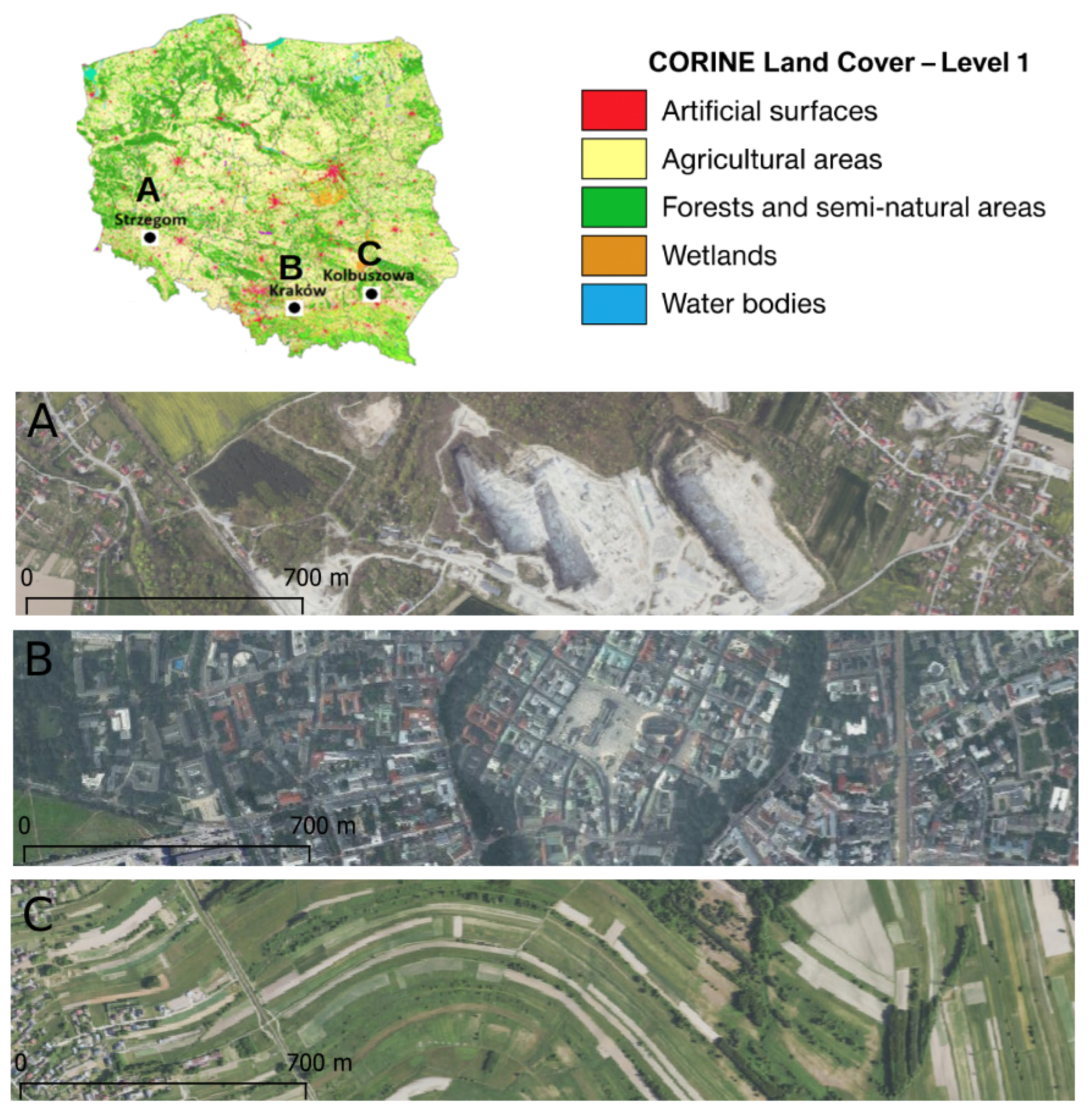
Figure 1. Three test areas presented on CORINE land use land cover map: (A) Strzegom—open-pit mine; (B) Kraków—urban; (C) Kolbuszowa—rural area in the south of Poland.
Applsci 15 09785 g001
Figure 2. Visualization of CORINE classes in our test area. A sample area 6 × 12 km with intensive exploitation located around the central point (50.9591 N, 16.3384 E, near Strzegom to the west). A small square covering mineral extraction sites, code 131, which is zoomed in on in Figure 3.
Applsci 15 09785 g002
Figure 3. Multi-temporal Sentinel-2 images—square from Figure 2; seasonal changes are visible in the area covered but not in vegetation. The goal was to train the neural network to differentiate and separate the exploitation area from bare soils and developed areas, while also classifying vegetation in both the growing and decaying phases.
Applsci 15 09785 g003
Figure 4. Example of image annotation: on the right are the original images, and on the left are the annotated images. Note that the same area may be annotated as a different class.
Applsci 15 09785 g004
Figure 5. Architecture of the U-Net model. The encoder path progressively reduces spatial resolution while increasing feature depth. The decoder path restores spatial resolution using upsampling and skip connections. The final output is a 1 × 9 pixel-wise class map (modified from [41]).
Applsci 15 09785 g005
Figure 6. Data processing workflow in U-Net, including input Sentinel-2 scenes, vector masks, and the 70/30 training–validation split for U-Net model training. Independent test data are reserved for final accuracy assessment.
Applsci 15 09785 g006
Figure 7. Example tensorboard registration.
Applsci 15 09785 g007
Figure 8. Loss function for various learning rate and weight decay values (CrossEntropyLoss).
Applsci 15 09785 g008
Figure 9. Accuracy for various configurations of class balancing, learning rate, and weight decay.
Applsci 15 09785 g009
Figure 10. Classification in GEE; in square brackets the number of points.
Applsci 15 09785 g010
Figure 11. Test classification of Strzegom (UTM 34N), UNET OA = 94.60% (modified after [41]).
Applsci 15 09785 g011
Figure 12. Test classification of Kolbuszowa (UTM 34N), UNET OA = 93.11% (modified after [41]).
Applsci 15 09785 g012
Figure 13. Location of mining sites operated without a license—red diamonds; green circle—the selected location (A); green rectangle—our test area Strzegom (B) (MOEK geoportal) (https://emgsp.pgi.gov.pl/emgsp/, accessed on 24 August 2025).
Applsci 15 09785 g013
Figure 14. Test area Strzegom—classification result; locations of geologically recognized deposits (exploited or not)—hatched polygons; examples of probable illegal exploitations—A and B on the Open Street Map.
Applsci 15 09785 g014
Figure 15. Test area Strzegom—black rectangle; location of geologically recognized deposits (exploited or not)—hatched polygons; examples of probable illegal exploitations—A and B on CORINE: A is located on 211: non-irrigated arable land; B on 112: discontinuous urban fabric.
Applsci 15 09785 g015
Figure 16. Confirmed illegal exploitation A; aerial photo 2014 (Google Earth).
Applsci 15 09785 g016
Figure 17. Illegal exploitation (A) stopped in 2020; aerial photo 2017 (Google Earth).
Applsci 15 09785 g017
Figure 18. Suspected illegal exploitation B, located outside the mining area (Monitoring of Open-pit Mineral Exploitation (MOEK)).
Applsci 15 09785 g018
Figure 19. Suspected illegal exploitation B, located on ‘112: Discontinuous urban fabric’ on CORINE but located within the area of documented mineral deposits in MIDAS.
Applsci 15 09785 g019
Figure 20. Strzegom test area and suspected illegal exploitation B, Class 10 U-Net classification.
Applsci 15 09785 g020
Figure 21. Suspected illegal exploitation B; aerial photo 2017 (Google Earth).
Applsci 15 09785 g021
Figure 22. Suspected illegal exploitation B; aerial photo 2018 (Google Earth).
Applsci 15 09785 g022
Figure 23. Suspected illegal exploitation B, in situ photo (Google Maps).
Applsci 15 09785 g023
Figure 24. Comparison of overall classification accuracy (OA) achieved by different models. U-Net outperformed classical machine learning methods in terms of pixel-wise classification accuracy.
Applsci 15 09785 g024
Table 3. Selected studies on LULC classification in agriculture areas using Sentinel-2 time series and deep learning.
Year/RefTask/DataMethod (NN)
Short Summary
2019 [32] LULC; Sentinel-2, 13 bandsCNN (ResNet-50, GoogLeNet)EuroSAT dataset (27k patches, 64 × 64 px, 10 classes). CNN benchmark; ResNet-50 (RGB) OA ≈ 98.6%. Standard LULC reference.
2020 [33] LULC/CAP; Sentinel-2 time seriesRNN (interpretability)CAP use case; explainability of RNNs; key bands and phenological stages identified.
2020 [28] Crops; Sentinel-2 TSI (10 bands)Pixel-Set Encoder + temporal attentionPixel-set + temporal self-attention; robust to clouds; reduced computation; SOTA accuracy.
2021 [34] Crops; dense Sentinel-2 series (with gaps)CNN/LSTM/GRUSequence models outperform classical ML without gap filling; robust to missing observations.
2022 [29] Crops; Sentinel-2 TSIDual-attention CNNSpectral + spatial attention; OA ≈ 98.5%, κ 0.98; exceeds RF/XGB/2D–3D CNNs.
2022 [35] Crops; Sentinel-2 TSI (Hetao, China)U-NetEarly crop ID via key phenological stages; earlier detection (e.g., sunflower ≈ 20 days sooner).
2023 [30] Crops; Sentinel-2 TSI (10 bands, 22 dates)A-BiGRU (attention)Gap reconstruction + attention; OA ≈ 98%, Macro-F1 ≈ 97.9%, κ 0.97; beats LSTM/SRNN.
Table 4. Comparison between the original U-Net [25] and the proposed model (BN: BatchNorm2d; skip-concat: concatenation with the corresponding encoder feature map).
ComponentOriginal U-NetProposed Model
Encoder blocks2 × (Conv3 × 3, ReLU); MaxPool2 × 23 × (Conv3 × 3, BN, ReLU); MaxPool2 × 2; padding = same
Bottleneck2 × (Conv3 × 3, ReLU)3 × (Conv3 × 3, BN, ReLU); padding = same
Decoder blocksConvTrans2 × 2; skip-concat; 2 × (Conv3 × 3, ReLU)ConvTrans2 × 2; ReplicationPad2d; skip-concat; 3 × (Conv3 × 3, BN, ReLU)
Table 5. Training configuration (fixed settings and sweep hyperparameters).
ItemValue
Classes1–9
Epochs25
Patch size100
Batch size4
Balance1
LossFocalLoss ( γ = 2 )
OptimizerAdam
Learning rate0.001
Weight decay (sweep){0.01, 0.001, 0.0001}
Gamma2
CUDAenabled
Table 6. Accuracy metrics commonly used in classification evaluation. More information on classification accuracy metrics, including definitions and practical examples, can be found in the companion repository: accuracy_checker GitHub repository (https://github.com/python-edu/accuracy_checker, accessed on 24 August 2025).
FormulaMetric Name
T P + T N T P + T N + F P + F N ACC (Accuracy)
T N T N + F P TNR (Specificity/True Negative Rate)
T P T P + T N + F P + F N OA (Overall Accuracy)
T P T P + F N PA (Producer Accuracy/Recall)
T P T P + F P UA (User Accuracy/Precision)
2 · P r e c i s i o n · R e c a l l P r e c i s i o n + R e c a l l F1-score
Table 7. Example confusion matrix for binary classification.
Actual/PredictedPositiveNegative
PositiveTP = 40FN = 10
NegativeFP = 5TN = 45
Total samples100
Table 8. Metric calculations for binary classification.
MetricCalculationResult
ACC = Accuracy 40 + 45 100 0.85
TNR = Specificity 45 45 + 5 0.90
OA = Overall Accuracy 40 + 45 100 0.85
PA = Recall 40 40 + 10 0.80
UA = Precision 40 40 + 5 0.89
F1-score 2 · 0.89 · 0.80 0.89 + 0.80 0.84 0.84
Table 9. Example confusion matrix for 3-class classification.
Actual/PredictedABC
A3055
B22810
C3522
Total samples110
Table 10. Binary confusion matrix components per class.
ClassTPFPFNTN
A3051065
B28101260
C2215865
Table 11. Per-class classification metrics.
ClassACCTNROAPA (Recall)UA (Precision)F1-Score
A0.8640.9290.72700.7500.8570.799
B0.8000.8570.72700.7000.7370.718
C0.7910.8130.72700.7330.5950.655
Table 12. Macro-averaged metrics across all classes.
MetricACCTNROAPA (Recall)UA (Precision)F1-Score
Mean0.8180.8660.72700.7280.7300.724
Table 13. Confusion matrix—Strzegom 20230709.
Class\Ref1234578910
112023636010110
25497568831030221353
300625223514020
4210147338133170187
5000611500000
700860590110
8010000635306
904325534067010,9271
1002802890406998
Table 14. Confusion matrix—Kolbuszowa 20210725 [41].
Class\Ref123456789
1110570100000
24215911960000
32032422402300
4009281345116503
50067212212200
6101021845530001
7001236010500
80010001210
915511210105001105
Table 15. Accuracy metrics for each class and Overall Accuracy—Strzegom 20230709.
ClassACCTNRPAUAF1
10.98420.98520.95470.68570.7981
20.97510.99720.89620.98890.9402
30.99460.99640.89540.82130.8568
40.97640.97720.97330.91190.9416
50.99320.99310.99480.81730.8974
70.99670.99740.70240.36880.4836
80.99890.99980.94490.99060.9673
90.97730.99230.94220.98140.9614
100.99640.99950.98270.99760.9901
Mean0.98810.99310.92070.84040.8707
Overall0.9464
Table 16. Accuracy metrics for each class and Overall Accuracy—Kolbuszowa 20210725 [41].
ClassACCTNRPAUAF1
10.99190.99170.99280.94120.9663
20.98180.98540.96480.93310.9487
30.98850.99360.86400.84820.8560
40.97200.97980.95490.95520.9550
50.98440.99190.93710.94870.9429
60.97270.98660.79100.81790.8042
70.98820.99030.83330.53570.6522
80.99981.00000.91301.00000.9545
90.98300.99950.87560.99640.9321
Mean0.98470.99100.90300.88630.8902
Overall0.9311
Table 17. Summary of classification results for GEE-based classifiers.
ModelOAPA (Recall)UA (Precision)F1-Score
CART (GEE)0.76790.77010.76720.7657
RF (GEE)0.80000.70980.72950.7100
SVM (GEE)0.78570.74210.73850.7241
Table 18. Accuracy metrics for each class and Overall Accuracy—CART.
ClassACCTNRPAUAF1
10.96430.97410.70000.50000.5833
20.93570.96730.71430.75760.7353
30.90360.92380.84290.78670.8138
40.89640.94290.75710.81540.7852
51.00001.00001.00001.00001.0000
70.92140.95380.50000.45450.4762
80.96790.98850.70000.82350.7568
90.95000.97200.76670.76670.7667
100.99641.00000.95001.00000.9744
Mean0.94840.96920.77010.76720.7657
Overall0.7679
Table 19. Accuracy metrics for each class and Overall Accuracy—RF.
ClassACCTNRPAUAF1
10.95710.96670.70000.43750.5385
20.95000.98370.71430.86210.7813
30.90710.90950.90000.76830.8289
40.92140.96190.80000.87500.8358
51.00001.00001.00001.00001.0000
70.93570.96150.60000.54550.5714
80.97141.00000.60001.00000.7500
90.96070.97600.83330.80650.8197
100.99641.00000.95001.00000.9744
Mean0.96000.97590.70980.72950.7100
Overall0.8000
Table 20. Accuracy metrics for each class and Overall Accuracy—SVM.
ClassACCTNRPAUAF1
10.97500.97411.00000.58820.7407
20.95360.97140.82860.80560.8169
30.88930.92380.78570.77460.7801
40.91790.97140.75710.89830.8217
51.00001.00001.00001.00001.0000
70.90360.91540.75000.40540.5263
80.97501.00000.65001.00000.7879
90.96070.99200.70000.91300.7925
100.99641.00000.95001.00000.9744
Mean0.95710.97480.74210.73850.7241
Overall0.7857
Table 21. Comparison between U-Net and GEE-based classification methods.
AspectU-Net (Deep Learning)GEE Classifiers (CART/RF/SVM)
Data ScopeMulti-region (Strzegom, Kolbuszowa, Kraków)Single-region (Strzegom only)
Model TypeConvolutional Neural Network (Semantic Segmentation)Classical ML (decision trees, SVM)
ImplementationPyTorch (local, offline)Google Earth Engine (cloud-based)
Input DataSentinel-2 patches (10 bands)Sentinel-2 scene (10 bands)
Training RegionsThree regionsOne region
Output TypePixel-wise segmentation mapPixel-wise classification labels
StrengthsHigh accuracy, generalization, robust to variabilityFast, simple to implement, no local resources needed
LimitationsRequires GPU, longer training time, more dataLimited generalization, lower precision in complex areas
Disclaimer/Publisher’s Note: The statements, opinions and data contained in all publications are solely those of the individual author(s) and contributor(s) and not of MDPI and/or the editor(s). MDPI and/or the editor(s) disclaim responsibility for any injury to people or property resulting from any ideas, methods, instructions or products referred to in the content.