Cost Analysis and Optimization of Modern Power System Operations

Abstract

The reliable and economical operation of modern power systems is increasingly complex due to the integration of diverse energy sources and dynamic load patterns. A critical challenge is maintaining the balance between electricity supply and demand within various operational constraints. This study addresses the economic scheduling of generation units using a Mixed Integer Programming (MIP) optimization model. Key constraints considered include reserve requirements, ramp rate limits, and minimum up/down time. Simulations are performed across multiple scenarios, including systems with spinning reserves, responsive demand, renewable energy integration, and energy storage systems. For each scenario, the optimal mix of generation resources is determined to meet a 24 h load forecast while minimizing operating costs. The results show that incorporating demand responsiveness and renewable resources enhances the economic efficiency, reliability, and flexibility of the power system.

1. Introduction

A basic strategy for meeting electricity demand is to keep all available generators online at all times; however, this strategy is highly uneconomical. A more efficient method involves committing only the required generating units during specific time periods, a process known as unit commitment [1]. The integration of renewable energy sources, Plug-in Electric Vehicles (PEVs), and energy storage systems has significantly enhanced the flexibility and resilience of power systems, but it has also increased the complexity of the unit commitment problem [2]. In addition, there has been a notable shift in operational strategy—from adjusting generation to follow demand, to actively managing demand in response to available supply. The adoption of responsive or flexible demand plays a significant role in reducing operating costs and enhancing system performance [3,4]. Efficient resource scheduling is critical not only for ensuring reliable electricity generation but also for improving system flexibility, resilience, and economic efficiency. These objectives are achieved by solving the unit commitment problem to minimize total operating cost while subject to key operational constraints such as ramp rate limits and reserve requirements [5,6,7]. Moreover, the global shift toward smart grid technologies—driven by increased penetration of renewables and energy storage—has introduced new paradigms in energy generation and consumption [8].

Due to the finite nature of non-renewable energy resources and their lasting environmental impacts, there is a growing global shift toward the integration of renewable energy sources and energy storage systems. With proper management and favorable weather conditions, renewable resources can significantly enhance the versatility and robustness of the power system. Furthermore, the cost of renewable energy has declined substantially in recent years, making it increasingly competitive with conventional resources [9,10]. As a result, the hybridization of renewable and traditional generation systems has been widely explored in the recent literature [11,12,13].

One of the most promising approaches for enhancing power system flexibility and efficiency is the implementation of demand-side flexibility measures, which target management of electricity consumption at the load side. Demand-side management (DSM) systems and efforts to reduce usage during peak periods can effectively lower the overall system load and lead to significant operational cost savings. This strategy accelerates the response time of power supply systems, enhancing flexibility while reducing both operational and capital expenditures [14,15,16]. Responsive loads—including residential and industrial consumers as well as PEVs—play a key role in supporting grid stability and contribute to improving the system’s flexibility and resilience [17,18]. In [19], PEVs are specifically highlighted as tools for enhancing grid flexibility.

Flexibility in power systems has been defined in multiple ways. In [20,21], it is described as the network’s capability to provide non-served energy, while [18] defines it as the system’s ability to respond rapidly to substantial and sudden changes in load. A framework for evaluating power system flexibility using load response and renewable resources is presented in [22]. Furthermore, the approach in [23] assesses system flexibility by incorporating fast-ramping generation units, responsive loads, and energy storage systems.

Numerous algorithms have been explored in [24,25] to address the complexities inherent in the unit commitment (UC) problem. Traditional approaches include methods such as priority listing, dynamic programming, Lagrangian relaxation, branch and bound, Mixed Integer Programming (MIP), and stochastic programming. In addition to these, a variety of intelligent optimization techniques have been applied, including artificial neural networks, binary-coded genetic algorithms, fuzzy logic, and particle swarm optimization.

In this study, the Mixed Integer Programming (MIP) approach is adopted for solving the UC problem due to its flexibility, high accuracy, and ability to model complex operational constraints. MIP is well-suited for large-scale problems and can produce globally optimal solutions. Nevertheless, it needs to be noted that computational complexity and tractability can become challenging for very large systems due to the combinatorial nature of mixed-integer formulations and specific features such as network topology, local operational policies, regional factors (e.g., market structure), and other elements that may require model customization.

The optimization is carried out using the General Algebraic Modelling System (GAMS), which offers a wide range of solvers and efficient computational performance, significantly reducing solution time. The MIP framework also supports the potential future enhancement of system adaptability through collaborative scheduling of different resources (e.g., PEVs, building temperature control systems), as suggested in [26]. To improve fairness, the framework can be enhanced to use quantified contributions (e.g., energy traded, flexibility) as bargaining powers—following the Nash bargaining method. This allows profit allocation to better reflect each subsystem’s actual value, beyond equal sharing [27].

The primary objective of this paper is to demonstrate the cost-saving potential of incorporating demand-side flexibility and to analyze how the integration of renewable energy sources and energy storage systems impacts overall operating costs.

2. Mathematical Formulation

Fuel costs, start-up costs, and shut-down costs constitute the three key operating cost components in any unit commitment problem. In the following section, a mathematical model for unit commitment cost calculation is developed, which forms the basis for the model implementation presented in the study. We start by minimizing the total cost of operation including fuel cost, shut-down cost, and start-up cost,

$$\mathit{min}\mathit{O}\mathit{F}=\sum _{\mathit{i},\mathit{t}}\mathit{F}{\mathit{C}}_{\mathit{i},\mathit{t}}+\mathit{S}\mathit{T}{\mathit{C}}_{\mathit{i},\mathit{t}}+\mathit{S}\mathit{D}{\mathit{C}}_{\mathit{i},\mathit{t}}$$

(1)

where fuel cost (FC) is given as follows,

$$\mathit{F}\mathit{C}\mathit{i}\left(\mathit{P}\mathit{i}\left(\mathit{t}\right)\right)=\mathit{A}\mathit{i}+\mathit{B}\mathit{i}\mathit{P}\mathit{i}\left(\mathit{t}\right)+\mathit{C}\mathit{i}{\mathit{P}\mathit{i}}^2(\mathit{t})$$

(2)

To ensure safe and efficient operation of any power system network, the supply provided should be greater than or equal to load demand at all available times, and is given by the following equation,

$$\sum _{\mathit{i}}\mathit{P} \mathit{i},\mathit{t}\ge \mathit{L} \mathit{t}$$

(3)

The above equations represent a basic form of unit commitment problem. However, in practical applications, additional physical, technical, and environmental limitations must be taken into account. The constraints typically considered in a unit commitment problem include minimum up/down time, ramp up/down time, minimum and maximum generating capacity, start-up/shut-down cost, running cost, fuel usage constraints, etc. To reduce the computational complexity of the optimization problem, the non-linear cost function is linearized using the following set of equations,

$$0\le {\mathit{p}}_{\mathit{i},\mathit{k}}^{\mathit{k}}\le \mathit{\Delta }{\mathit{P}}_{\mathit{i}}^{\mathit{k}} {\mathit{u}}_{\mathit{i},\mathit{t}} ,\forall \mathit{k}=1:\mathit{n}$$

(4)

$$∆{\mathit{P}}_{\mathit{i}}^{\mathit{k}}= {\displaystyle \frac{{\mathit{P}}_{\mathit{i}}^{\mathit{m}\mathit{a}\mathit{x}}-{\mathit{P}}_{\mathit{i}}^{\mathit{m}\mathit{i}\mathit{n}}}{\mathit{n}}}$$

(5)

$${\mathit{P}}_{\mathit{i},\mathit{i}\mathit{n}\mathit{i}}^{\mathit{k}}=\left(\mathit{k}-1\right)∆{\mathit{P}}_{\mathit{i}}^{\mathit{k}}+{\mathit{P}}_{\mathit{i}}^{\mathit{m}\mathit{i}\mathit{n}}$$

(6)

$${\mathit{P}}_{\mathit{i},\mathit{f}\mathit{i}\mathit{n}}^{\mathit{k}}=∆{\mathit{P}}_{\mathit{i}}^{\mathit{k}}+{\mathit{P}}_{\mathit{i},\mathit{i}\mathit{n}\mathit{i}}$$

(7)

$${\mathit{P}}_{\mathit{i},\mathit{t}}={\mathit{P}}_{\mathit{i}} {\mathit{u}}_{\mathit{i},\mathit{t}}+ \sum _{\mathit{k}}{\mathit{P}}_{\mathit{i},\mathit{t}}^{\mathit{k}}$$

(8)

$${\mathit{s}}_{\mathit{i}}^{\mathit{k}}= {\displaystyle \frac{{\mathit{C}}_{\mathit{i},\mathit{f}\mathit{i}\mathit{n}}^{\mathit{k}}-{\mathit{C}}_{\mathit{i}.\mathit{i}\mathit{n}\mathit{i}}^{\mathit{k}}}{∆{\mathit{P}}_{\mathit{i}}^{\mathit{k}}}}$$

(9)

$$\mathit{F}\mathit{C}\mathit{i},\mathit{t}={\mathit{a}}_{\mathit{i}}{\left(\mathit{P}{\mathit{i}}^{\mathit{m}\mathit{i}\mathit{n}}\right)}^2+{\mathit{b}}_{\mathit{i}} \mathit{P}{\mathit{i}}^{\mathit{m}\mathit{i}\mathit{n}}+{\mathit{c}}_{\mathit{i}} {\mathit{u}}_{\mathit{i},\mathit{t}} + \sum _{\mathit{k}}{\mathit{s}}_{\mathit{i}}^{\mathit{k}} {\mathit{P}}_{\mathit{i},\mathit{t}}^{\mathit{k}}$$

(10)

Constraints in power systems represent a range of technical and environmental restrictions that must be satisfied to ensure reliable and safe operation; failure to comply can result in significant operational issues. For this study, the following constraints are considered:

• Ramp Rate Constraint: The increment and decrement in power output of generator per hour in spinning mode is called ramp rate. It is given by % per hour or MW per hour. For the ith unit at time t, the ramp rate constraints are given as follows,

$${\mathit{P}\mathit{\prime }}_{\mathit{i},\mathit{t}}\le {\mathit{P}}_{\mathit{i},\mathit{t}}\le {\mathit{P}\mathit{″}}_{\mathit{i},\mathit{t}}$$

(11)

$${\mathit{P}\mathit{″}}_{\mathit{i},\mathit{t}} \le {\mathit{P}}_{\mathit{i}}^{\mathit{m}\mathit{a}\mathit{x}} \left[ {\mathit{u}}_{\mathit{i},\mathit{t}}-{\mathit{z}}_{\mathit{i},\mathit{t}+1}\right]+\mathit{S}\mathit{D}\mathit{i} {\mathit{z}}_{\mathit{i},\mathit{t}+1}$$

(12)

$${\mathit{P}\mathit{″}}_{\mathit{i},\mathit{t}}\le {\mathit{P}}_{\mathit{i},\mathit{t}-1}+\mathit{R}\mathit{U}\mathit{i} {\mathit{u}}_{\mathit{i},\mathit{t}}+\mathit{S}\mathit{U}\mathit{i} {\mathit{y}}_{\mathit{i},\mathit{t}}$$

(13)

$${\mathit{P}\mathit{\prime }}_{\mathit{i},\mathit{t}} \ge {\mathit{P}}_{\mathit{i},\mathit{t}}^{\mathit{m}\mathit{i}\mathit{n}} {\mathit{u}}_{\mathit{i},\mathit{t}}$$

(14)

$${\mathit{P}\mathit{\prime }}_{\mathit{i},\mathit{t}} \ge {\mathit{P}}_{\mathit{i},\mathit{t}-1}-\mathit{R}\mathit{D}\mathit{i} {\mathit{u}}_{\mathit{i},\mathit{t}}-\mathit{S}\mathit{D}\mathit{i} {\mathit{z}}_{\mathit{i},\mathit{t}}$$

(15)

• Minimum Up/Down time constraint: Due to physical and technical restrictions, a generator cannot be shut down or restarted instantaneously. Minimum Up/Down time represents the smallest time interval required that the generating unit must remain online or offline once started up or shut down, respectively. To model these constraints, three integer decision variables are introduced for each generating unit at each time period: u_i,t (operational status: ON/OFF), y_i,t (startup status), and z_i,t (shut-down status). The three integer decision variables are governed by the following equations,

$${\mathit{y}}_{\mathit{i},\mathit{t}}-{\mathit{z}}_{\mathit{i},\mathit{t}}={\mathit{u}}_{\mathit{i},\mathit{t}} -{\mathit{u} }_{\mathit{i},\mathit{t}-1}$$

(16)

$${\mathit{y}}_{\mathit{i},\mathit{t}} +{\mathit{z}}_{\mathit{i},\mathit{t}} \le 1$$

(17)

$${\mathit{y}}_{\mathit{i},\mathit{t}} ,{\mathit{z}}_{\mathit{i},\mathit{t}} ,{\mathit{u}}_{\mathit{i},\mathit{t}}\in \left\{\mathrm{0,1}\right\}$$

(18)

The minimum up time (UTi) for the ith unit is given as follows,

$$\sum _{\mathit{t}=\mathit{k}}^{\mathit{\varsigma }\mathit{i}}1-{\mathit{u}}_{\mathit{ i},\mathit{t}}=0$$

(19)

$$\sum _{\mathit{t}=\mathit{k}}^{\mathit{k}+\mathit{U}\mathit{T}\mathit{i}-1}{\mathit{u}}_{\mathit{i},\mathit{t}}\ge \mathit{U}\mathit{T}\mathit{i}{\mathit{y}}_{\mathit{i},\mathit{k}},\forall \mathit{k}=\mathit{\varsigma }\mathit{i}+1\dots \mathit{T}-\mathit{U}\mathit{T}\mathit{i}+1$$

(20)

$$\sum _{\mathit{t}=\mathit{k}}^{\mathit{T}}{\mathit{u}}_{\mathit{i},\mathit{t}}-{\mathit{y}}_{\mathit{i},\mathit{t}}\ge 0,\forall \mathit{k}=\mathit{T}-\mathit{U}\mathit{T}\mathit{i}+2\dots \mathit{T}$$

(21)

$${\mathit{\varsigma }}_{\mathit{i}}=\mathit{min}\{\mathit{T},\left(\mathit{U}\mathit{T}\mathit{i}-{\mathit{U}}_{\mathit{i}}^0\right){\mathit{u}}_{\mathit{i},\mathit{t}=0}\}$$

(22)

The minimum down time (DTi) for the ith unit is given as follows,

$$\sum _{\mathit{t}=1}^{\mathit{\xi }\mathit{i}}{\mathit{u}}_{\mathit{i},\mathit{t}}=0$$

(23)

$$\sum _{\mathit{t}=\mathit{k}}^{\mathit{k}+\mathit{D}\mathit{T}\mathit{i}-1}1-{\mathit{u}}_{\mathit{i},\mathit{t}}\ge \mathit{D}\mathit{T}\mathit{i} {\mathit{z}}_{\mathit{i},\mathit{k}} ,\forall \mathit{k}=\mathit{\xi }\mathit{i}+1\dots .\mathit{T}-\mathit{D}\mathit{T}\mathit{i}+1$$

(24)

$$\sum _{\mathit{t}=\mathit{k}}^{\mathit{T}}1-{\mathit{u}}_{\mathit{i},\mathit{t}}-{\mathit{z}}_{\mathit{i},\mathit{t}}\ge 0,\forall \mathit{k}=\mathit{T}-\mathit{D}\mathit{T}\mathit{i}+2\dots .\mathit{T}$$

(25)

$$\mathit{\xi }\mathit{i}=\mathit{m}\mathit{i}\mathit{n}\{\mathit{T},(\mathit{D}\mathit{T}\mathit{i}-{\mathit{S}}_{\mathit{i}}^0 \left)\right[1-{\mathit{u}}_{\mathit{i},\mathit{t}=0}\left]\right\}$$

(26)

• Start-Up/Shut-Down Cost: This cost is incurred for starting up and shutting down any generating unit from the system and is modelled by the help of the following equations,

$$\mathit{S}\mathit{T}{\mathit{C}}_{\mathit{i},\mathit{t}}=\mathit{C}{\mathit{s}}_{\mathit{i}}{\mathit{y}}_{\mathit{i},\mathit{t}}$$

(27)

$$\mathit{S}\mathit{D}{\mathit{C}}_{\mathit{i},\mathit{t}}=\mathit{S}{\mathit{d}}_{\mathit{i} }{\mathit{z}}_{\mathit{i},\mathit{t}}$$

(28)

The flowchart shown in Figure 1 outlines the coding logic implemented in the GAMS Integrated Development Environment (IDE) for simulating the proposed system [28,29]. The process begins with defining various input sets such as the time horizon, generator indices, and cost segments. Once these sets are established, technical and economic data for each generator—such as cost coefficients, minimum and maximum generation capacities, and ramp rates—are provided in tabular form.

Subsequently, functions are developed to automatically retrieve the required parameters during each simulation cycle. The next step involves inputting hourly load data for the defined time horizon, along with the corresponding electricity prices associated with meeting that load. Following this, various decision variables are declared. Binary variables include u (i, t), y (i, t), and z (i, t), while positive variables represent parameters such as start-up cost, shut-down cost, and generator output levels at each time step t.

After variable declarations, all operational constraints—such as ramp rate limits, minimum up/down time, generation-load balance, and demand flexibility—are formulated using standard equation syntax supported by GAMS 24.9.1. Once the objective function, variables, and constraints are fully defined, an appropriate solver must be selected. GAMS offers a range of solvers such as ALPHAECP, AMPL, BDML, and LINDOGLOBAL12.0, among others.

It is crucial to include all relevant equations in the solve command; otherwise, the solver will ignore omitted constraints. Upon execution, the solver iterates through various generator combinations to meet the load demand while minimizing total operating cost. The output includes generator schedules, associated start-up and shut-down costs, and a summary of the total operating cost, typically presented in tabular format.

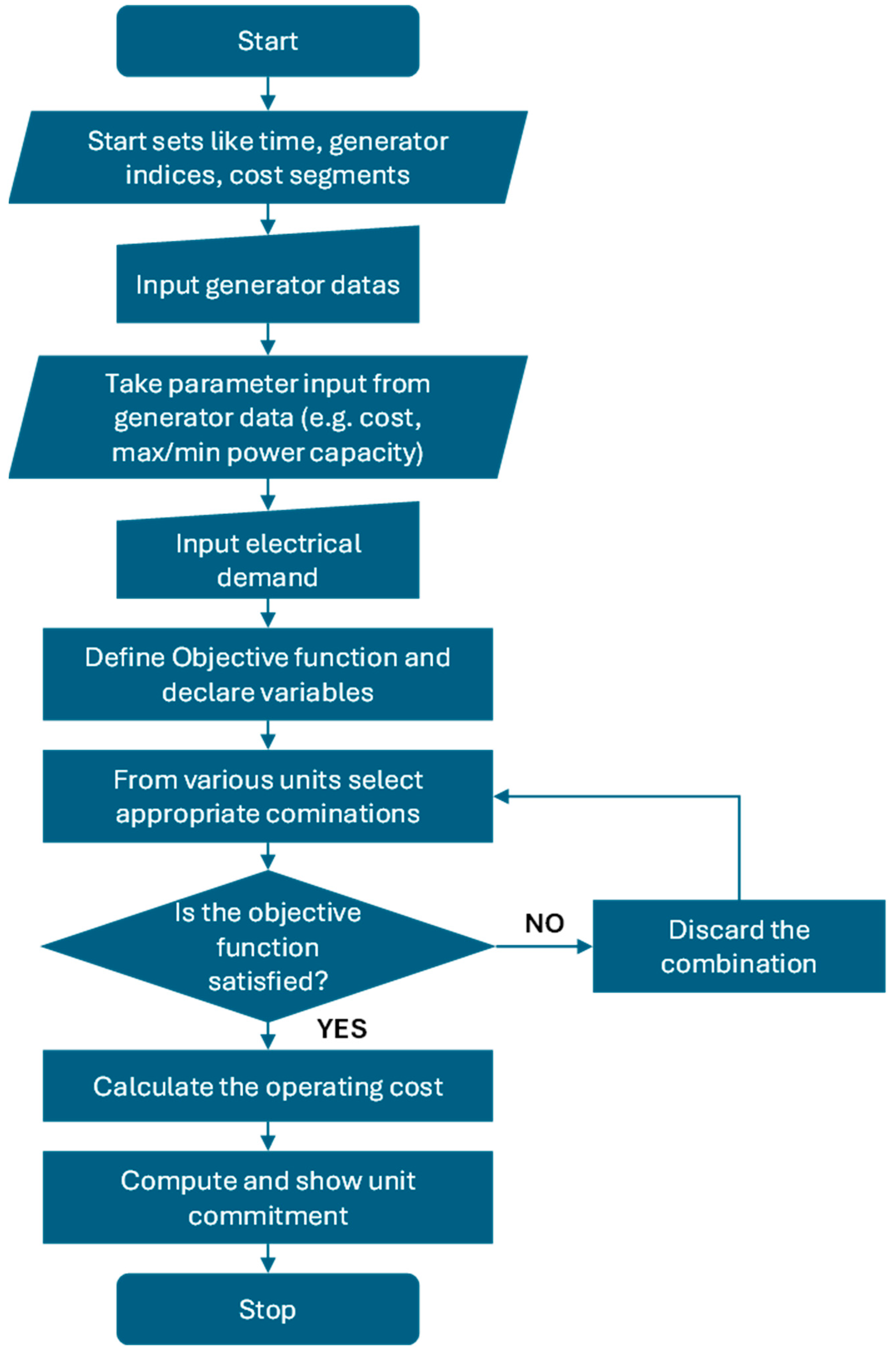
3. Implementation and Case Studies

To implement the unit commitment algorithm, the essential input parameters include generator characteristics, hourly electrical demand, and electricity supply prices [30]. Since the study focuses on a day-ahead scheduling scenario, 24 h data for both demand and electricity prices are required. The algorithm processes these inputs to determine the optimal on/off status of each generator and calculates the total system operating cost.

In this study, the system comprises 10 thermal generating units. The key characteristics of each generator—such as minimum and maximum generation capacity, ramp-up and ramp-down limits, start-up and shutdown costs, and generation cost coefficients—are considered for the optimization. These parameters are summarized in the following

Table 1. Data of thermal generators.

Unit	a ($/MW2)	b ($/MW)	c ($)	CostSD ($)	costst ($)	RU (MW/h)	RD (MW/h)	UT (h)	DT (h)	SD (MWh)	SU (MWh)	Pmin (MW)	Pmax (MW)	U0 (h)	Uini (h)	S0 (h)
g1	0.0149	12.1	82.0	42.6	42.6	40	40	3	2	90	110	80	200	1	0	1
g2	0.0289	12.6	50.6	50.6	50.6	64	64	4	3	130	140	120	320	2	0	2
g3	0.0135	13.2	100.0	57.1	57.1	30	30	3	2	70	80	50	150	3	0	3
g4	0.0127	13.9	105.0	47.9	47.9	104	104	5	3	240	250	250	520	0	3	0
g5	0.0261	15.0	72.0	56.6	56.6	56	56	4	2	110	130	100	280	1	0	0
g6	0.0212	29.0	141.5	141.5	141.5	30	30	2	2	60	80	50	150	0	0	0
g7	0.0382	32.0	100.0	57.1	57.1	60	60	3	2	45	55	30	110	0	0	0
g8	0.0393	30.0	100.0	57.1	57.1	30	30	3	2	45	55	30	110	0	0	0
g9	0.0396	15.0	25.0	50.6	50.6	22	22	3	2	35	45	20	100	0	0	0
g10	0.051	14.3	15.0	57.1	57.1	12	12	0	0	30	40	20	60	0	0	0

.

In the given table information about different cost coefficients, Start-up/Shut-down cost, Up-time/Down-time, Ramp Up/Down rates, Shut-down/Start-Up rate, and minimum and maximum capacity of different generating units are given. Also, in the above table additional information about duration of time for which a unit has been ON/OFF at the beginning of the operating horizon is given under parameters U_o/S_o. As the study is conducted for the next 24 h scheduling of available generating units, information about load demand for 24 h is also required for simulation, hence data for load demand (L_t) are given as Figure 2.

Figure 2 presents the dynamic load profile over the 24 h operating horizon, reflecting the varying electricity demand throughout the day [31]. The load fluctuates significantly, with a minimum observed demand of 834 MW and a peak of 1455 MW. This variation highlights the importance of optimal unit commitment to ensure cost-effective and reliable power system operation.

Figure 3 illustrates that electricity prices fluctuate throughout the 24 h operational period rather than remaining constant [32]. The lowest electricity prices are observed during the early hours (from t1 to t6), while the highest prices occur during the intervals t7 to t10 and t17 to t23, reflecting periods of peak demand or constrained supply.

This study is structured into four distinct case studies, each addressing a different system scenario or operational constraint:

1.

Case 1—Base Scenario (Traditional System):

The unit commitment problem is solved for a conventional power system comprising 10 thermal generating units. The technical and economic characteristics of these units are detailed in Table 1.

2.

Case 2—Reserve Constraint:

In this scenario, a reserve constraint is introduced in addition to the standard unit commitment constraints. This enhancement is aimed at improving the system’s reliability by ensuring adequate spinning reserves are maintained.

3.

Case 3—Integration of Renewables and Storage:

To evaluate the benefits of a more flexible power system, this case incorporates renewable energy sources and energy storage systems alongside the existing thermal generation units. The objective is to assess how modern generation technologies impact operational cost and system performance.

4.

Case 4—Demand Flexibility:

This scenario explores the impact of demand-side flexibility on the system’s operating cost. Different levels of demand flexibility are considered to quantify potential cost savings and improvements in system responsiveness.

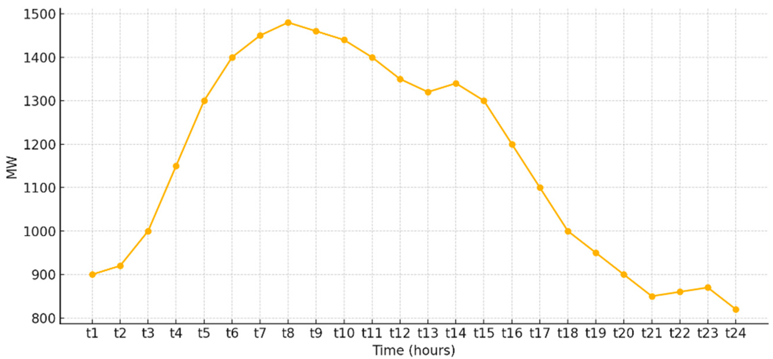
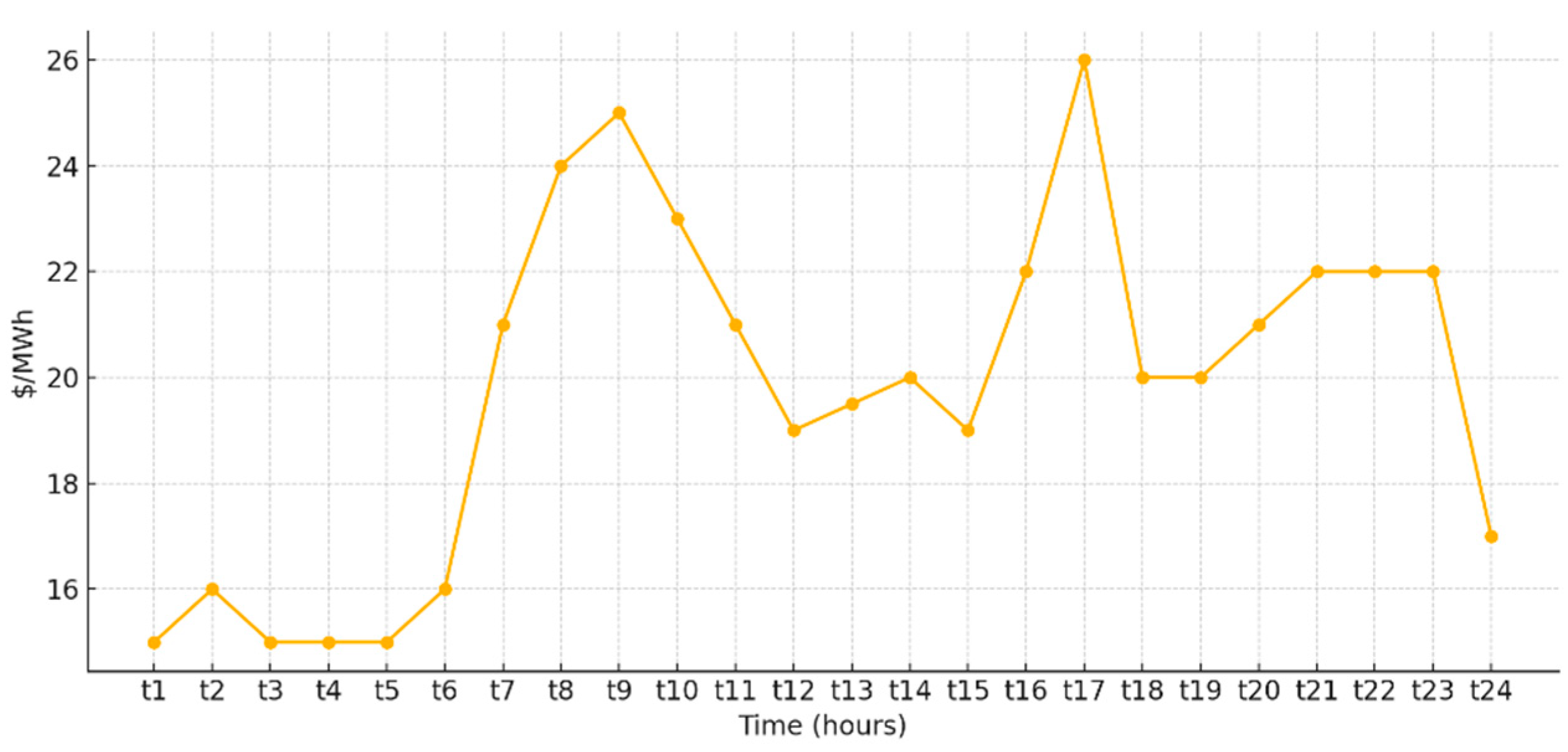
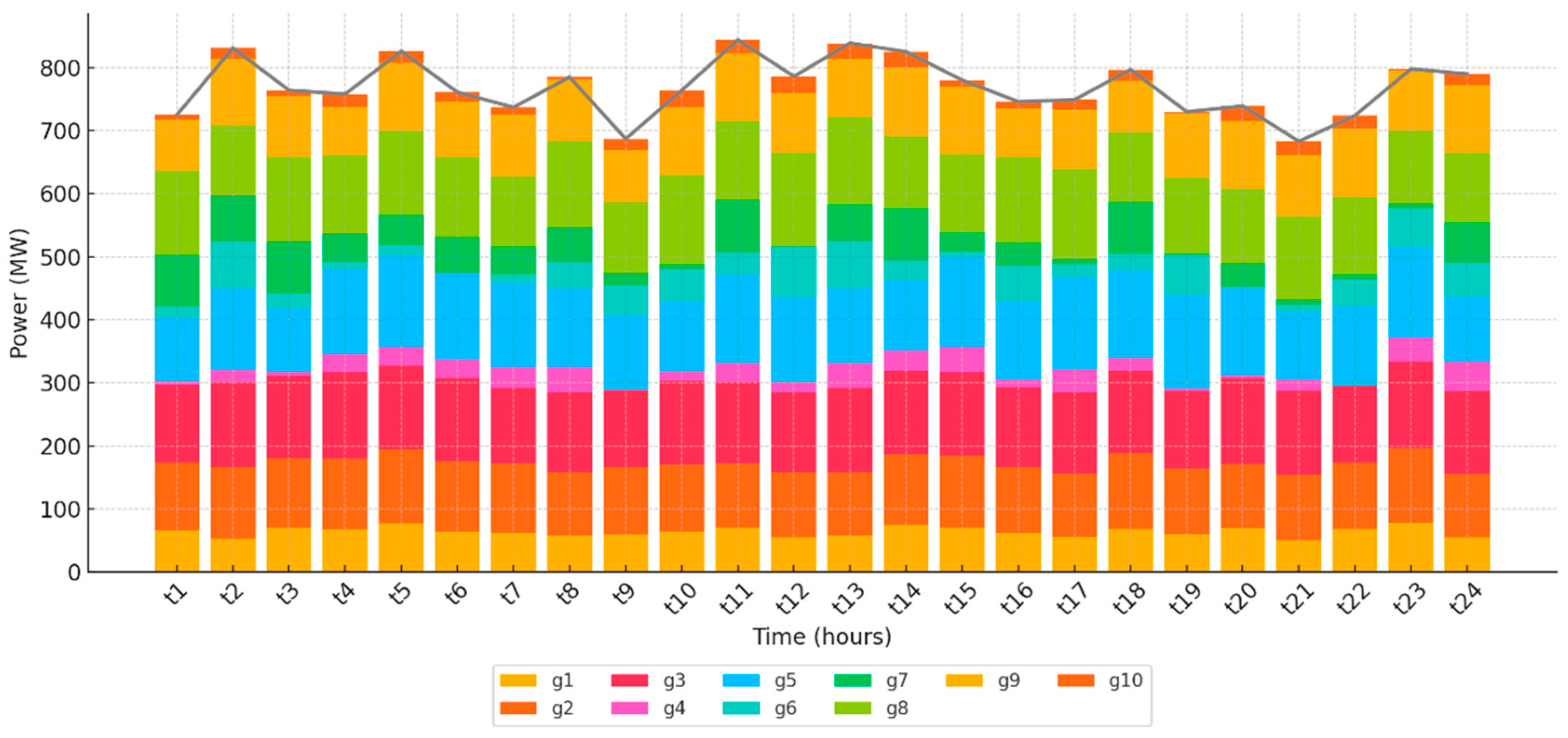
3.1. Case 1: Unit Commitment of 10 Thermal Power Plants for Dynamic Load

In this case study, the unit commitment problem is implemented using the GAMS platform for a system comprising 10 thermal generating units, whose operational datasets are provided in Table 1. The system is operated over a 24 h period under a dynamic load profile, as depicted in Figure 4. The primary objective is to minimize the total operating cost, which includes the fuel cost, start-up cost, and shut-down cost, as represented by the cost function in Equation (1).

To solve the problem, a Mixed Integer Programming (MIP) formulation is employed. Several operational constraints are incorporated into the model, including

• Ramp rate limits
• Minimum up/down time requirements
• Power balance between supply and demand
• Start-up and shut-down cost constraints

The binary decision variables used in the model are

• u(i,t): Indicates the ON/OFF status of generator i at time t
• y(i,t): Indicates the start-up status of generator i at time t
• z(i,t): Indicates the shutdown status of generator i at time t
• In addition to binary variables, positive continuous variables are defined:
• p(i,t): Power output of generator i at time t
• StC(i,t): Start-up cost of generator i at time t
• SdC(i,t): Shutdown cost of generator i at time t

Once the model is fully defined, GAMS solves the optimization problem using one of its MIP-compatible solvers. After simulation, the resulting generator schedules—including the operational status and output of each generator over the 24 h period—are obtained and presented as follows.

One of the primary advantages of solving the unit commitment problem is the ability to operate the power system economically by selecting an optimal subset of available generating units, rather than running all units simultaneously. This strategic selection ensures that demand is met at the lowest possible operating cost, while still adhering to system constraints.

As illustrated in Figure 4, at time step t1, the system demand of 883 MW is met without utilizing generators g1, g2, g6, and g8. Instead, the load is supplied by an optimal combination of units: g3, g4, g5, g7, g9, and g10. This selection highlights the efficiency of unit commitment in minimizing operational costs by prioritizing generators with lower cost coefficients, favorable ramp rates, or more suitable startup conditions at that hour.

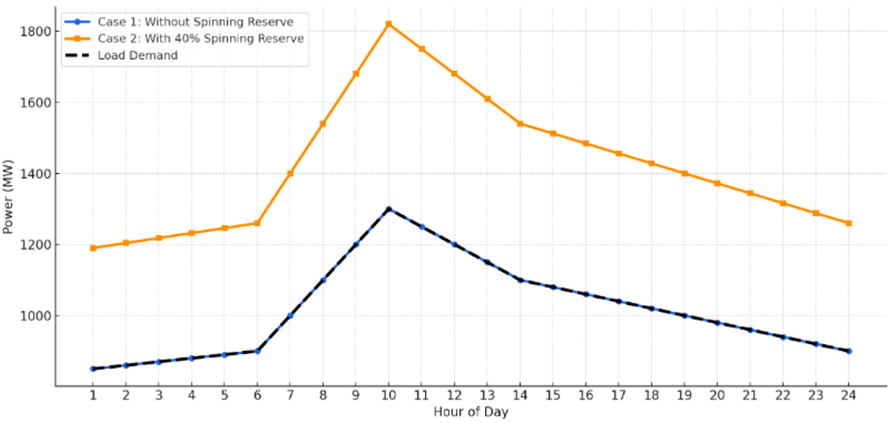
3.2. Case 2: Unit Commitment of 10 Thermal Power Plants for Given Dynamic Load with Spinning Reserve Constraints

In the previous case, a basic unit commitment problem was formulated and solved. However, real-world power systems are subject to uncertainties and unforeseen events, such as generator outages or sudden load changes. To enhance the reliability and robustness of unit commitment solutions, an additional constraint—namely the spinning reserve constraint—must be introduced.

Spinning reserve (SR) refers to the immediately available extra capacity from online units that can be dispatched on short notice to respond to system disturbances. It is defined as the difference between a generator’s maximum available capacity and its current output. Spinning reserves are critical for improving the security, flexibility, and dependability of the power system.

In this case study, the objective function remains unchanged: minimizing the total operating cost, which includes fuel, start-up, and shut-down costs. The only modification is the inclusion of the spinning reserve constraint in addition to the existing constraints such as ramp rate limits, minimum up/down times, and power balance.

The spinning reserve constraint can be mathematically expressed and implemented in GAMS as follows:

$$\mathit{R}\mathit{i},\mathit{t}\le {\mathit{P}}^{\mathit{m}\mathit{a}\mathit{x}}\mathit{i},\mathit{t}-\mathit{P}\mathit{i},\mathit{t}$$

(29)

$${\displaystyle \sum _{\mathit{i}=1}^{\mathit{n}}}\mathit{R}\mathit{i},\mathit{t}\ge \mathit{\gamma }\mathit{L}\mathit{t}$$

(30)

where R_i,t is the reserve provision by the ith unit at time t and $P^{max}i,t$ maximum amount of power that can be supplied by a unit, and P_i,t is the power supplied by the ith unit at time t. In a power system, the reserve requirement is fixed as a percentage of demand, and that is defined by Equation (30), where $\mathit{\gamma }$ is the % of load demand that specifies the reserve requirement and L_t is load demand at time t. For this study, $\mathsf{\gamma }=\mathbf{40}\mathit{\%}$, and the load is decreased by 55% of the load taken in case 1. It is important to note that while the spinning reserve does not reduce total system load in the conventional sense, it reduces load-carrying and commitment requirements within the power system, resulting in reduced overall load needs. A study of adding the potential effect of adding spinning reserves in the case of Spanish islands found system cost reductions of up to 30% of overall system cost, in extreme cases resulting in more than 50% of thermal generation reduction. While significantly reducing operational costs, spinning reserves will result in higher overall system investments and related costs [32]. After simulation and optimization on GAMS using the mixed integer programming technique, the generator schedule and reserve provision are as Figure 5.

Spinning reserve available for 24 h is shown as Figure 6.

As illustrated in Figure 5, an optimal combination of thermal generators is dispatched to meet the 24 h load demand while ensuring system reliability. The inclusion of spinning reserve, visualized in Figure 6, provides additional operational flexibility and security.

For instance, at time step t2, generators g4, g5, and g7 contribute spinning reserves of 99.1 MW, 38.6 MW, and 27 MW, respectively—after meeting their allocated portion of the load demand. This unused generation capacity represents reserve power that is immediately available to the system.

Such spinning reserves play a crucial role in enhancing the dependability of the power system. They can be deployed to

• Cover sudden increases in load,
• Compensate for unexpected drops in renewable generation, or
• Respond to generator outages or other unforeseen contingencies.

The integration of spinning reserves into the unit commitment strategy thus ensures not only economic operation but also operational resilience in dynamic power system environments.

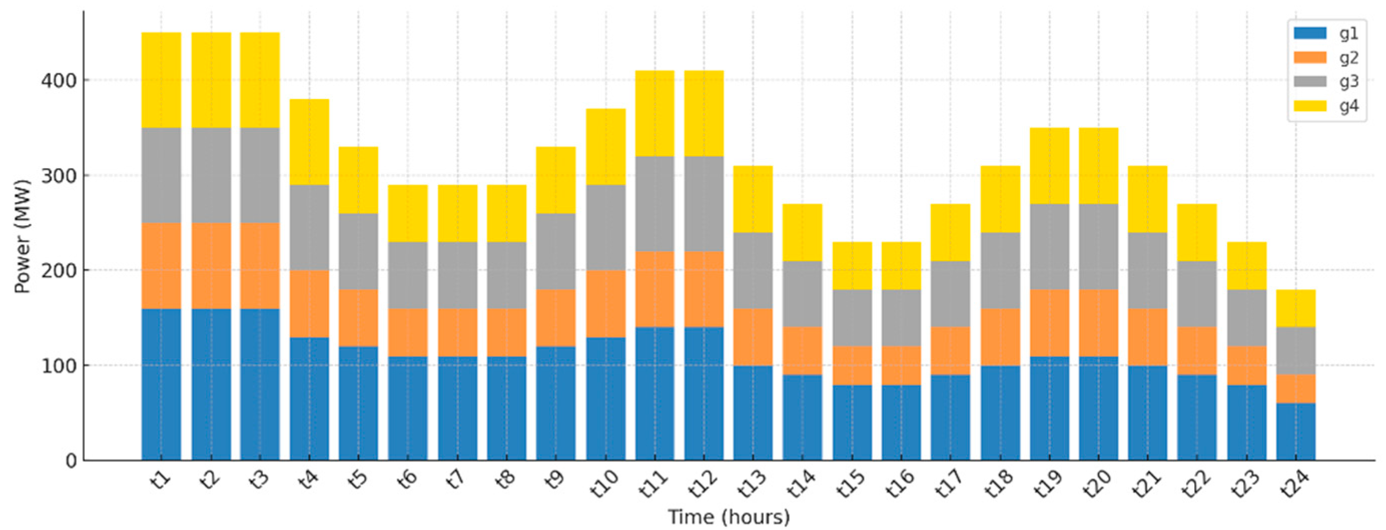
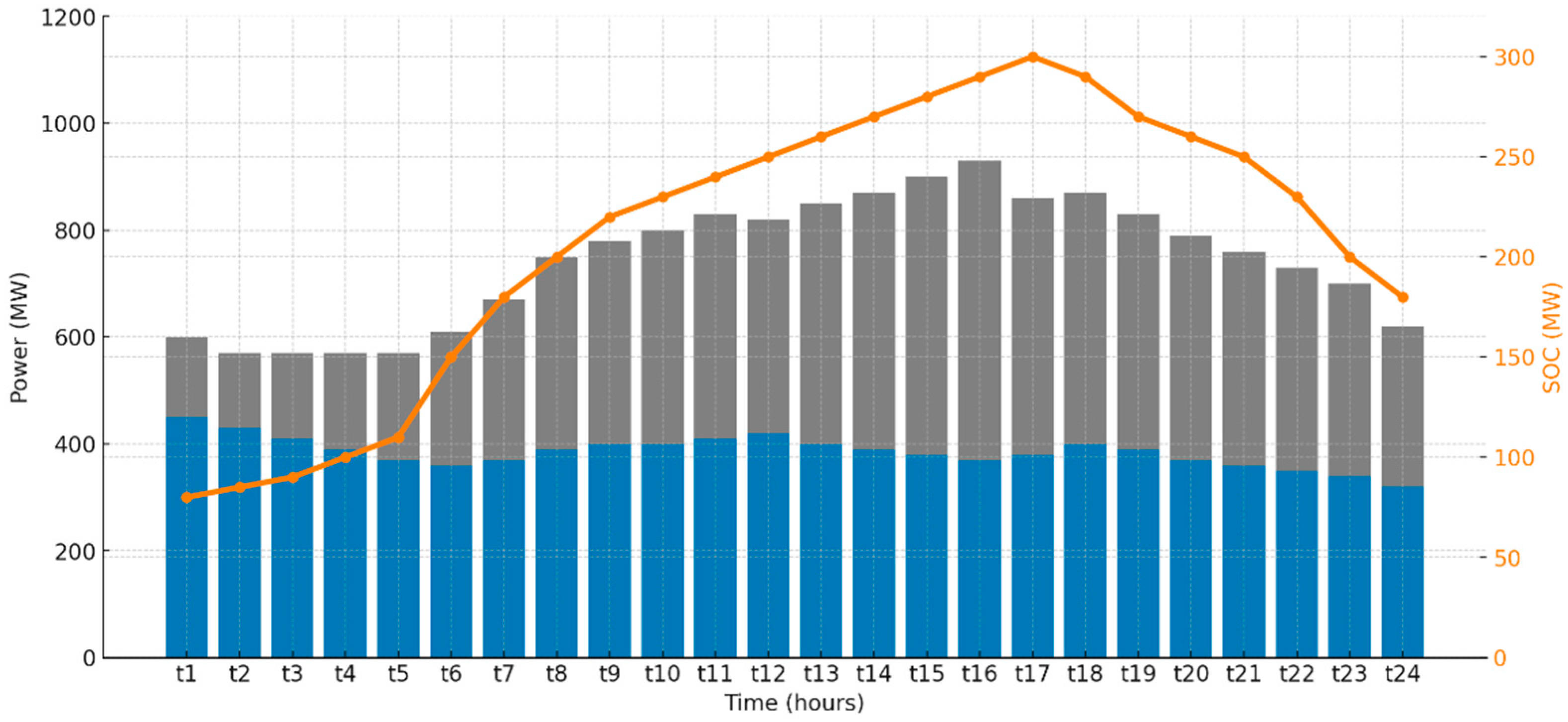
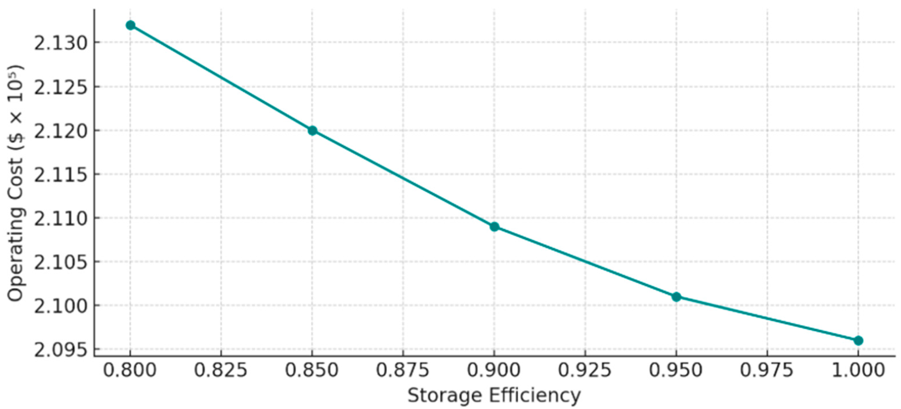
3.3. Case 3: Unit Commitment of Thermal Units with Energy Storage System and Wind Energy for 24 h Dynamic Load

In this case, a modern power system is studied that supplies electricity to consumers using a hybrid mix of thermal power plants, renewable energy resources, and energy storage systems (ESS). For this analysis, only four thermal generating units are considered, in addition to wind energy and battery storage systems.

The decision to include only four thermal units reflects current trends in the energy sector, where the global push to reduce greenhouse gas emissions and combat climate change is driving a transition away from fossil fuels—particularly coal-fired power plants—and toward clean energy alternatives. As such, this model represents a more sustainable and environmentally responsible approach to power system planning.

The inclusion of renewables and ESS significantly enhances the flexibility of the power system. Energy storage allows for demand-side flexibility, supporting a shift to the supply-driven demand paradigm. This means that instead of adjusting generation to match demand, demand can now be managed or shifted to align with available supply—especially from intermittent sources like wind.

However, this increased flexibility also introduces greater system complexity, particularly in balancing variability and ensuring reliability. Therefore, solving the unit commitment problem remains critical for ensuring efficient and smooth operation of the power system.

Since wind energy is a part of the generation portfolio in this case, the estimated 24 h wind energy availability profile is provided as Figure 7.

As shown in Figure 7, wind energy availability is intermittent and varies significantly throughout the 24 h period. This intermittency presents challenges for reliable power system operation. To address this, modern power systems incorporate energy storage systems (ESS), which help smooth out fluctuations by storing surplus energy during periods of low demand or low prices and releasing it during high demand or high price periods.

For this study, a battery energy storage system (BESS) is employed. The system is characterized by the following parameters:

• Maximum state of charge (SOCₘₐₓ): 300 MW
• Initial state of charge (SOC₀): 100 MW at the start of the operating horizon
• Minimum charging/discharging power: 0 MW
• Maximum charging/discharging power: 0.2 × SOCₘₐₓ = 60 MW

Like all real-world technologies, storage systems are not 100% efficient. For this study:

• Charging efficiency: 95%
• Discharging efficiency: 90%

To accurately capture the behavior and cost implications of integrating wind energy and battery storage, the objective function is modified. In addition to minimizing traditional operating costs (fuel, startup, and shutdown), the revised objective function now includes a wind energy curtailment penalty. This ensures that any unused or curtailed wind energy is factored into the economic assessment, encouraging maximum utilization of available renewable resources.

The updated objective function is given as follows:

$$\mathit{min}\mathit{O}\mathit{F}=\sum _{\mathit{i},\mathit{t}}\mathit{F}\mathit{C}\mathit{i},\mathit{t}+\mathit{S}\mathit{T}\mathit{C}\mathit{i},\mathit{t}+\mathit{S}\mathit{D}\mathit{C}\mathit{i},\mathit{t}+\sum _{\mathit{t}}\mathit{V}\mathit{W}\mathit{C}\times \mathit{P}\mathit{w}$$

(31)

Also, some additional constraints and modifications are performed, such as,

$$\mathit{S}\mathit{O}{\mathit{C}}_{\mathit{m}\mathit{i}\mathit{n}} \left(60 \mathit{M}\mathit{W}\right)<\mathit{S}\mathit{O}{\mathit{C}}_{\mathit{t}}<\mathit{S}\mathit{O}{\mathit{C}}_{\mathit{m}\mathit{a}\mathit{x}} (300 \mathit{M}\mathit{W})$$

(32)

$${\mathit{P}}_{\mathit{t}}^{\mathit{w}}+\sum {\mathit{P}}_{\mathit{g},\mathit{t}}+{\mathit{P}}_{\mathit{t}}^{\mathit{d}}\ge {\mathit{L}}_{\mathit{t}}-{\mathit{P}}_{\mathit{t}}^{\mathit{c}}$$

(33)

After modifying and including the above three equations, the unit commitment algorithm is applied in GAMS for this case, and the following outputs are found at Figure 8.

As illustrated in Figure 8, the operation of the Energy Storage System (ESS) plays a critical role in balancing supply and demand throughout the 24 h horizon. For instance, at time t1, the ESS discharges 10 MW to help meet the load demand, compensating for a shortfall in power from both renewable and thermal generation sources. Conversely, at time t6, the ESS charges 60 MW, effectively storing excess energy that is not immediately required to meet demand.

This ability to shift energy temporally—absorbing surplus generation during low-demand periods and releasing it during high-demand or supply-deficient periods—contributes to significant operational cost savings. Moreover, the inclusion of ESS enhances the flexibility and resilience of the power system by reducing reliance on expensive peaking units and minimizing renewable energy curtailment.

Overall, the strategic use of storage enables a more efficient, economical, and reliable power system, especially in systems with high penetration of intermittent renewable resources. Figure 9 depicts the schedule of four generating units in a day.

The MIP-based optimization model presented in this study is generalizable in structure, but its practical applicability and scalability do depend on system characteristics such as grid size, complexity, and regional regulations. The core MIP formulation is suitable for small to medium-sized power systems, such as regional grids, microgrids, or isolated networks. However, for very large-scale power systems (e.g., national grids with thousands of units and buses), the computational burden can grow rapidly due to the increase in binary and continuous variables. In such cases, decomposition methods or heuristic/metaheuristic strategies may be preferred to balance accuracy and tractability. The current model assumes a homogeneous regulatory and market structure, which may not apply in regions with diverse energy policies, pricing mechanisms (e.g., nodal vs. zonal), or priority dispatch rules (e.g., renewable priority feed-in). Adapting the model for specific regions would require customizing constraints such as emission caps, reserve sharing protocols, or market-clearing rules. Figure 10 represents the unit commitment of a day in case 3.

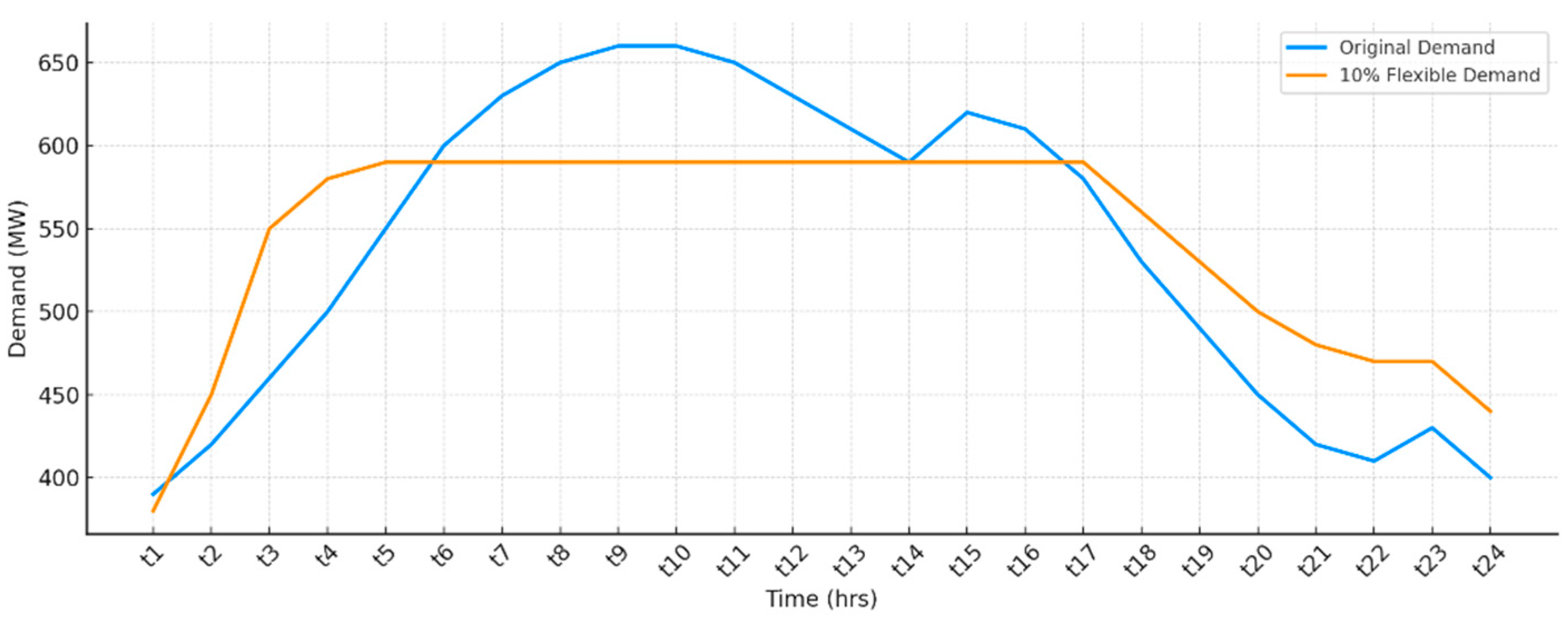
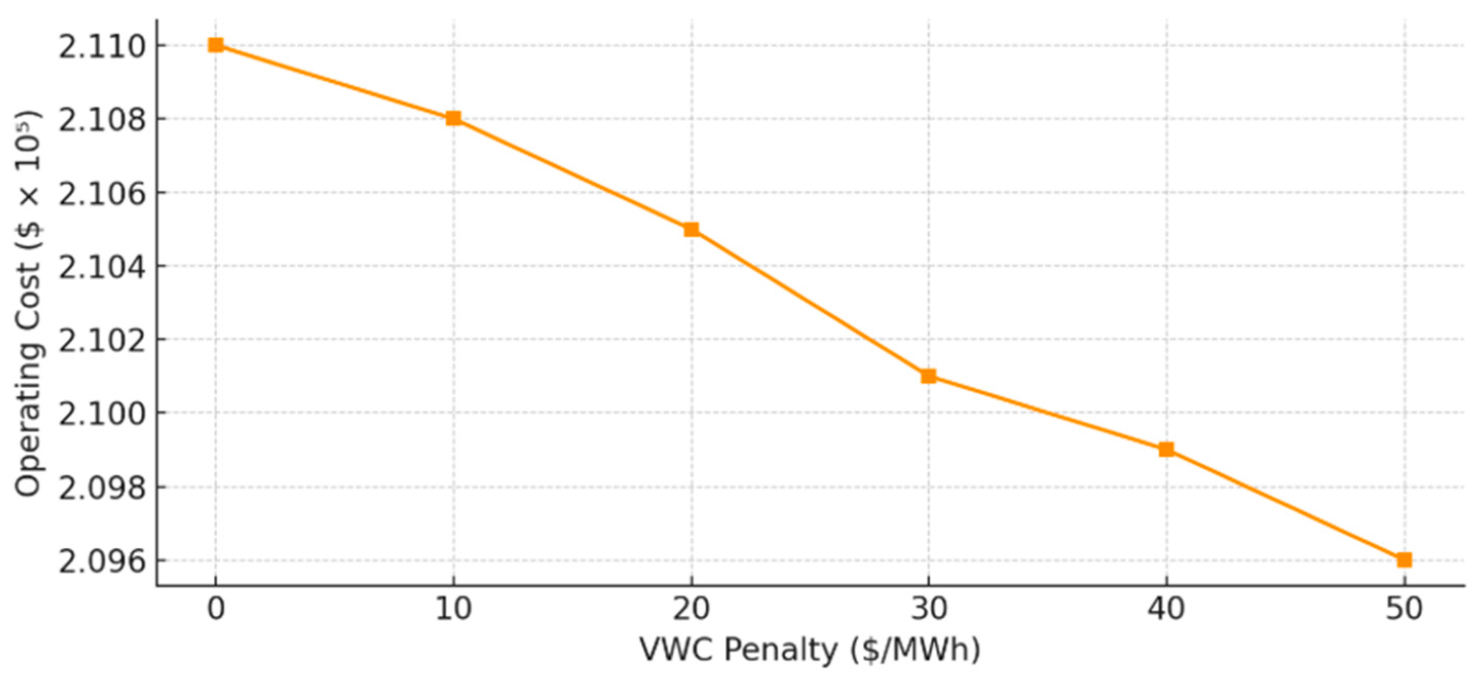
3.4. Case 4: Unit Commitment Demand Flexibility Constraint

In this case, demand-side flexibility (DSF) is investigated as a mechanism to improve the operational efficiency and economics of power systems. Demand-side flexibility refers to the extent to which electricity demand can be reduced, increased, or shifted within a given time window in response to supply conditions, market signals, or system constraints.

Traditionally, power systems have relied heavily on supply-side management, where generation is adjusted to match demand in real time. However, with the rise of smart grids, the integration of information and communication technologies (ICT), and the deployment of smart appliances and devices at the consumer end, it is now increasingly feasible to also manage demand in a dynamic and coordinated way.

In this study, the focus is on analyzing how operating costs vary with the degree of demand-side flexibility. Flexibility can be introduced both

• At the consumer side through demand response programs and smart appliances,
• And at the supply side via technologies like battery energy storage systems (BESS).

To model demand-side flexibility within the unit commitment problem, additional constraints are introduced to allow demand shifting and modulation across the 24 h horizon. These constraints govern

• Maximum allowable deviation from baseline demand (upward or downward),
• Temporal balancing to ensure total shifted demand is met within the operational window,
• And potential cost penalties or incentives associated with shifting loads.

It is good to note that for sustainable resource participation in demand flexibility, fairness and ongoing incentivization must be maintained. For that, contribution-based sharing mechanisms that distribute collective benefits (cost savings or revenues through program participation) are preferred [32].

The mathematical formulation of these constraints is provided in the following section.

$$\left(1-\mathit{\varsigma }\mathit{m}\mathit{i}\mathit{n}\right)\mathit{L}\mathit{t}\le \mathit{D}\mathit{t}\le \left(1+\mathit{\varsigma }\mathit{m}\mathit{a}\mathit{x}\right)\mathit{L}\mathit{t}$$

(34)

$$\sum _{\mathit{t}}\mathit{D}\mathit{t}=\sum _{\mathit{t}}\mathit{L}\mathit{t}$$

(35)

where ς_min/max determines min/max demand flexibility. For study, ς_min/max in this case is taken between 0 to 20%. Figure 11 depicts the comparison of flexible demand and actual demand.

In this case, for different values of demand flexibility, operating cost is calculated and shown in Figure 12 below.

4. Results and Discussion

This paper presents a comprehensive analysis of four distinct case studies for solving the unit commitment (UC) problem in a power system, aimed at determining the optimal day-ahead scheduling of generating units to meet dynamic load demand while minimizing operating costs.

• Case 1 examines a traditional power system with 10 thermal units, resulting in an operating cost of USD 4.8524 × 10⁵, with fuel, start-up, and shut-down costs amounting to USD 484,797, USD 442.1, and USD 0, respectively. This forms the baseline for comparison.
• Case 2 incorporates spinning reserve requirements (assumed at 40%) for enhanced reliability. With a 55% load reduction, the operating cost drops significantly to USD 2.1090 × 10⁵, and start-up/shut-down costs are reduced to USD 199.4 and USD 213.4, respectively, highlighting the cost of maintaining reserve margins.
• Case 3 transitions to a modern power system configuration, involving only four thermal units, wind energy, and an energy storage system (ESS). This integration results in a notably lower operating cost of USD 2.2336 × 10⁵, emphasizing both economic efficiency and enhanced flexibility from renewables and ESS.
• Case 4 explores the impact of demand-side flexibility (DSF). By enabling 10% demand flexibility, the system achieves a further cost reduction to USD 2.0965 × 10⁵, demonstrating the potential of smart grid technologies and responsive consumption in optimizing operations.

The results of the case analysis are summarized in

Table 2. Summary of results of case analysis.

Scenario	Operating Cost ($)	Energy Storage System Usage	Avoided Emissions	Flexibility Level
Base Scenario	485,240	None	Baseline	Low
Reserve Constraint (Spinning Reserve)	210,900	None (Spinning Reserves maintained)	Improved reliability (not quantified)	Medium (Spinning Reserve)
Renewables + Storage	223,360	Battery Energy Storage System (ESS)	Reduced (due to renewables)	High (Storage + Renewables)
Demand Flexibility	209,650	Demand-side flexibility (possible storage support)	Reduced (due to demand flexibility)	Highest (Demand Flexibility)

below.

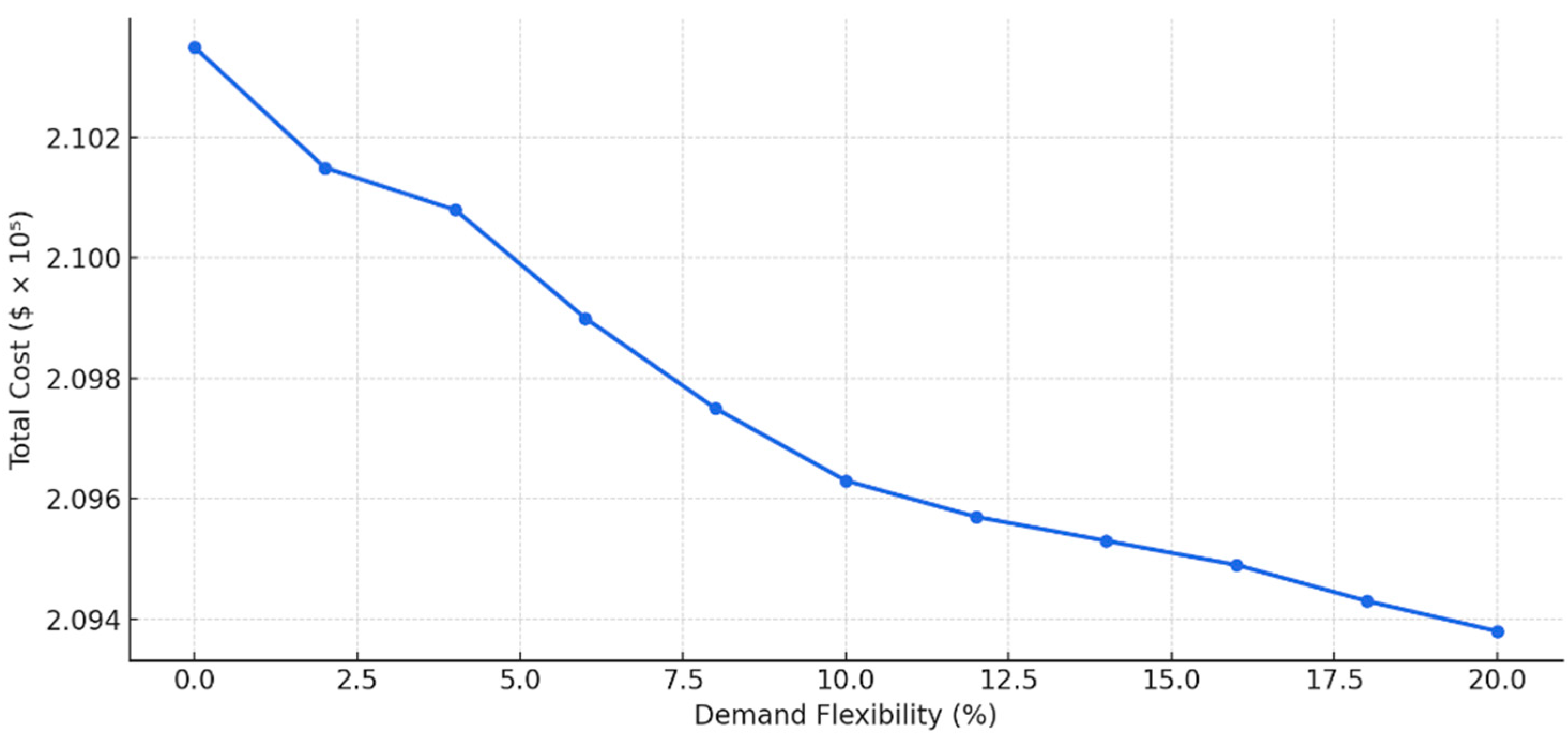
5. Sensitivity Analysis

To evaluate the robustness of the optimization results, a sensitivity analysis was conducted on two key parameters: energy storage efficiency and wind curtailment penalty (VWC).

Storage Efficiency: As shown in Figure 13, increasing storage efficiency from 80% to 100% significantly reduces operating costs, indicating that storage system performance has a strong influence on economic outcomes.

Wind Curtailment Penalty: Figure 14 demonstrates that increasing the penalty for curtailed wind energy encourages the system to utilize more renewable power, leading to lower overall operating costs. This suggests that properly pricing curtailment can incentivize greater renewable integration.

These results underscore the importance of accurate parameter selection and the economic value of enhancing storage performance and curtailment handling strategies.

6. Comparison of Case 1 and Case 2 at Same Load

We have reformulated Case 2 to use the same 24 h dynamic load profile as Case 1. The only difference now is the addition of the spinning reserve constraint, set at 40% of hourly load demand, as originally described. This modification allows us to isolate and quantify the cost impact of spinning reserve provision. The results now show that with the spinning reserve constraint applied, the total operating cost increases by approximately 6.9%, rising from USD 485,240 (Case 1) to USD 518,765 (Case 2) for the same demand profile. This cost includes both fuel and reserve-related startup commitments.

Figure 15 clearly shows how the addition of a 40% spinning reserve increases the generation commitment beyond the baseline load demand.

7. Key Insights

• Unit commitment optimization significantly reduces operating costs when properly modelled with realistic system constraints.
• Incorporating spinning reserves improves system reliability but requires additional generation margin and slightly increases startup/shutdown costs.
• Renewables and ESS not only reduce fuel dependence but also enhance system flexibility and lower costs.
• Demand-side management, even with modest flexibility, presents a powerful tool for achieving both economic and operational benefits.

Overall, the study concludes that a flexible, intelligently managed power system—leveraging modern technologies and renewable resources—offers a more economical, reliable, and sustainable energy future.

8. Conclusions

This study proposes an optimization-based approach for solving the unit commitment (UC) problem in both traditional and modern power system networks. The Mixed Integer Programming (MIP) technique is utilized due to its high modelling accuracy, global optimality, and flexibility in handling system constraints. The problem is implemented using GAMS software over a 24 h operational horizon, and simulations are conducted across four distinct scenarios. Comparative analysis across these case studies highlights the economic and operational benefits of transitioning to flexible and renewable-integrated power systems.

Key Findings

• Integration of renewable energy resources leads to a significant reduction in fossil fuel-based power generation and overall operating cost, promoting both economic and environmental benefits.
• Energy Storage Systems (ESS) play a crucial role in enhancing power system flexibility. Their ability to shift energy temporally allows better integration of variable renewable generation and supports grid stability.
• From both the generation and demand perspective, ESS becomes increasingly important with higher levels of renewable penetration. This reduces the fuel consumption of thermal units, contributing to lower operational costs.
• The use of ESS and renewables also aids in mitigating the environmental impact of conventional generation and enhances energy security by reducing dependency on fossil fuels.
• The study of demand-side flexibility (Case 4) reveals that even modest levels of flexibility (e.g., 10%) lead to notable reductions in operating costs, highlighting the value of smart appliances and consumer responsiveness in modern grid operations.

References

1. Padhy, N.P. Unit commitment—A Bibliographical Survey. IEEE Trans. Power Syst. 2004, 19, 1196–1205. [Google Scholar] [CrossRef]
2. Mollahassani-pour, M.; Rashidinejad, M.; Abdollahi, A. Spinning reserve contribution using unit responsibility criterion incorporating preventive maintenance scheduling. Int. J. Electr. Power Energy Syst. 2015, 73, 508–515. [Google Scholar] [CrossRef]
3. Bouffard, F.; Ortega-Vazquez, M. The value of operational flexibility in power systems with significant wind power generation. In Proceedings of the 2011 IEEE Power and Energy Society General Meeting, Detroit, MI, USA, 24–29 July 2011; pp. 1–5. [Google Scholar]
4. Abu-Sharkh, S.; Arnold, R.J.; Kohler, J.; Li, R.; Markvart, T.; Ross, J.N.; Yao, R. Can microgrids make a major contribution to UK energy supply? Renew. Sustain. Energy Rev. 2006, 10, 78–127. [Google Scholar] [CrossRef]
5. Soshinskaya, M.; Crijns-Graus, W.H.; Guerrero, J.M.; Vasquez, J.C. Microgrids: Experiences, barriers and success factors. Renew. Sustain. Energy Rev. 2014, 40, 659–672. [Google Scholar] [CrossRef]
6. Lasseter, R.H. Microgrids. In Proceedings of the 2002 IEEE Power Engineering Society Winter Meeting, New York, NY, USA, 27–31 January 2002; Volume 1, pp. 305–308. [Google Scholar]
7. Liang, H.; Zhuang, W. Stochastic modeling and optimization in a microgrid: A survey. Energies 2014, 7, 2027–2050. [Google Scholar] [CrossRef]
8. Peesapati, R.; Yadav, V.K.; Kumar, N. Flower pollination algorithm based multi-objective congestion management considering optimal capacities of distributed generations. Energy 2018, 147, 980–994. [Google Scholar] [CrossRef]
9. Klyapovskiy, S.; You, S.; Cai, H.; Bindner, H.W. Incorporate flexibility in distribution grid planning through a framework solution. Int. J. Electr. Power Energy Syst. 2019, 111, 66–78. [Google Scholar] [CrossRef]
10. Lehtola, T.; Zahedi, A. Solar energy and wind power supply supported by storage technology: A review. Sustain. Energy Technol. Assess. 2019, 35, 25–31. [Google Scholar] [CrossRef]
11. Alirezazadeh, A.; Rashidinejad, M.; Abdollahi, A.; Afzali, P.; Bakhshai, A. A new flexible model for generation scheduling in a smart grid. Energy 2020, 191, 116438. [Google Scholar] [CrossRef]
12. Yang, Z.; Li, K.; Niu, Q.; Xue, Y. A comprehensive study of economic unit commitment of power systems integrating various renewable generations and plug-in electric vehicles. Energy Convers. Manag. 2017, 132, 460–481. [Google Scholar] [CrossRef]
13. Shahbazitabar, M.; Abdi, H. A novel priority-based stochastic unit commitment considering renewable energy sources and parking lot cooperation. Energy 2018, 161, 308–324. [Google Scholar] [CrossRef]
14. Miller, L.; Carriveau, R. Energy demand curve variables–An overview of individual and systemic effects. Sustain. Energy Technol. Assess. 2019, 35, 172–179. [Google Scholar] [CrossRef]
15. Zhang, B.; Kezunovic, M. Impact on power system flexibility by electric vehicle participation in ramp market. IEEE Trans. Smart Grid 2015, 7, 1285–1294. [Google Scholar] [CrossRef]
16. Schachter, J.A.; Mancarella, P.; Moriarty, J.; Shaw, R. Flexible investment under uncertainty in smart distribution networks with demand side response: Assessment framework and practical implementation. Energy Policy 2016, 97, 439–449. [Google Scholar] [CrossRef]
17. Lannoye, E.; Flynn, D.; O’Malley, M. Evaluation of power system flexibility. IEEE Trans. Power Syst. 2012, 27, 922–931. [Google Scholar] [CrossRef]
18. Papaefthymiou, G.; Grave, K.; Dragoon, K. Flexibility Options in Electricity Systems; Project number: POWDE14426; Ecofys: Utrecht, The Netherlands, 2014. [Google Scholar]
19. Roukerd, S.P.; Abdollahi, A.; Rashidinejad, M. Probabilistic-possibilistic flexibility-based unit commitment with uncertain negawatt demand response resources considering Z-number method. Int. J. Electr. Power Energy Syst. 2019, 113, 71–89. [Google Scholar] [CrossRef]
20. Nikoobakht, A.; Aghaei, J.; Shafie-Khah, M.; Catalao, J.P. Assessing increased flexibility of energy storage and demand response to accommodate a high penetration of renewable energy sources. IEEE Trans. Sustain. Energy 2018, 10, 659–669. [Google Scholar] [CrossRef]
21. Kumar, V.; Naresh, R.; Singh, A. Investigation of solution techniques of unit commitment problems: A review. Wind Eng. 2021, 45, 1689–1713. [Google Scholar] [CrossRef]
22. Alirezazadeh, A.; Rashidinejad, M.; Afzali, P.; Bakhshai, A. A new flexible and resilient model for a smart grid considering joint power and reserve scheduling, vehicle-to-grid and demand response. Sustain. Energy Technol. Assess. 2021, 43, 100926. [Google Scholar] [CrossRef]
23. Sachan, S.; Gupta, C.P. Analysis of contingent conditions in power system. In Proceedings of the 2014 Students Conference on Engineering and Systems, Allahabad, India, 28–30 May 2014; pp. 1–5. [Google Scholar] [CrossRef]
24. Sachan, S.; Mishra, S.; Øyvang, T.; Bordin, C. Minimizing active power losses and voltage deviations for reactive power planning considering bus vulnerability. Next Res. 2025, 2, 100633. [Google Scholar] [CrossRef]
25. Mccarl, B.A.; Meeraus, A.; Van der Eijk, P.; Bussieck, M.; Dirkse, S.; Steacy, P.; Nelissen, F. McCarl GAMS User Guide; GAMS Development Corporation: Washington, DC, USA, 2014. [Google Scholar]
26. Liu, L.; Xu, Y.; Kirschen, D.S.; Zhang, Y.; Zhao, J. Reliability-constrained optimal scheduling of multi-microgrid systems with aggregate spinning reserve determination. IEEE Trans. Transp. Electrif. 2025, 11. early access. [Google Scholar]
27. Ding, B.; Li, Z.; Li, Z.; Xue, Y.; Chang, X.; Su, J.; Sun, H. Cooperative operation for multiagent energy systems integrated with wind, hydrogen, and buildings: An asymmetric Nash bargaining approach. IEEE Trans. Ind. Inform. 2025, 21, 6410–6421. [Google Scholar] [CrossRef]
28. Ademovic, A.; Bisanovic, S.; Hajro, M. A genetic algorithm solution to the unit commitment problem based on real-coded chromosomes and fuzzy optimization. In Proceedings of the Melecon 2010—2010 15th IEEE Mediterranean Electro technical Conference, Valletta, Malta, 26–28 April 2010; pp. 1476–1481. [Google Scholar]
29. Carrion, M.; Arroyo, J.M. A computationally efficient mixed-integer and linear formulation and for the thermal and unit. IEEE Trans Power Syst. 2006, 21, 1371–1378. [Google Scholar] [CrossRef]
30. Sachan, S. Integration of electric vehicles with optimum sized storage for grid connected photo-voltaic system. AIMS Energy 2017, 5, 997–1012. [Google Scholar] [CrossRef]
31. Sachan, S.; Deb, S.; Singh, S.N. Different charging infrastructures along with smart charging strategies for electric vehicles. Sustain. Cities Soc. 2020, 60, 102238. [Google Scholar] [CrossRef]
32. Sachan, S.; Deb, S.; Singh, S.N.; Singh, P.P.; Sharma, D.D. Planning and operation of EV charging stations by chicken swarm optimization driven heuristics. Energy Convers. Econ. 2021, 2, 91–99. [Google Scholar] [CrossRef]
Figure 1. Flowchart for the proposed code logic.
Applsci 15 08481 g001
Figure 2. Electrical demand for 24 h taken for study.
Applsci 15 08481 g002
Figure 3. Electricity prices for 24 h taken for study.
Applsci 15 08481 g003
Figure 4. Power schedules of 10 generating units for dynamic load for 24 h.
Applsci 15 08481 g004
Figure 5. Power schedules of 10 generating units for given dynamic load for 24 h considering reserve provision.
Applsci 15 08481 g005
Figure 6. Reserve provision by thermal units for 24 h.
Applsci 15 08481 g006
Figure 7. Availability of wind energy for 24 h.
Applsci 15 08481 g007
Figure 8. Dispatch of energy storage system for 24 h.
Applsci 15 08481 g008
Figure 9. Schedule of four thermal generating units for 24 h.
Applsci 15 08481 g009
Figure 10. Unit commitment for 24 h in Case 3.
Applsci 15 08481 g010
Figure 11. Comparison between original demand and 10% flexible demand.
Applsci 15 08481 g011
Figure 12. The variation in total operating cost vs. demand side flexibility.
Applsci 15 08481 g012
Figure 13. The variation in storage efficiency vs. operating cost.
Applsci 15 08481 g013
Figure 14. The variation in wind curtailment penalty vs. operating cost.
Applsci 15 08481 g014
Figure 15. Generation schedules vs. load demand—Case 1 and Case 2 (same load).
Applsci 15 08481 g015