The Forecast of the Wind Turbine Generated Power Using Hybrid (LTC + XGBoost) Model

Abstract

This publication presents a novel approach to predicting the amount of electricity generated by wind power plants. The research focuses on data-driven models such as XGBoost, Liquid Time-constant Networks, and covers both the analysis of properties of individual forecasting models as well as aspects of their integration into a hybrid model. By analyzing real-world weather scenarios, the approach aims to identify the highest accuracy forecasting model for the short-term 24-h forecast of wind farm power output. A more accurate forecast allows for more efficient resource planning and better distribution of resources on the electricity grids, thus ensuring a greener approach to energy production. The study shows that the proposed Hybrid (XGBoost + LTC) model predicts wind power generation with an nMAE of 0.0856, representing an improvement over standalone XGBoost and LTC models, and outperforming classical approaches such as LSTM and statistical models like ARIMAX in terms of forecasting accuracy.

1. Introduction

The growing urgency of climate change mitigation and the pursuit of sustainable economic growth have placed renewable energy development at the forefront of global energy strategies. Among these, wind power has emerged as a particularly promising solution due to its clean, renewable, and increasingly cost-competitive nature [1]. As fossil fuels are gradually phased out, ensuring a stable and resilient electricity supply based on renewable sources requires precise planning and reliable forecasting techniques.

In Europe, the European Union’s “Strategy for Energy System Integration” [2] outlines ambitious goals—such as producing at least 80% of heat from renewables and electrifying 80% of public transport by 2050 [3,4,5]. In Lithuania, significant strides have already been made in this direction. In 2022, for the first time, more than 60% of electricity produced in the country came from renewable sources, including wind, solar, hydropower, ambient heat, biomass, and biofuels [6]. Despite this milestone, achieving Lithuania’s national goal of producing 90% of electricity locally by 2030 [7] will require continuous expansion of renewable energy capacity and the integration of advanced operational technologies.

Wind energy plays a crucial role in Lithuania’s renewable energy portfolio due to the country’s favorable geographical conditions, especially in its western regions. However, as the share of wind power in the national grid increases, so does the system’s exposure to its variability and intermittency. Unlike conventional power plants, wind turbines cannot be dispatched on demand, and their output is subject to rapid fluctuations in meteorological conditions. Additionally, electricity generated from wind cannot be stored directly in large quantities using cost-effective means [8,9,10], which complicates integration into real-time electricity markets and power system operations.

Accurate short-term forecasting of wind power—particularly within a 24-h horizon—is therefore vital for maintaining grid stability, minimizing imbalance penalties, optimizing market bids, and ensuring the efficient use of resources. This is especially relevant in markets such as Nord Pool, where energy producers are expected to submit precise day-ahead production forecasts. Improved forecasts can reduce the need for expensive reserves, prevent curtailments, and support decision-making in both grid operation and energy trading.

To address these challenges, this research aims to create a data analysis and prediction model that could produce accurate short-term predictions of wind farm power output for the next 24 h. Analysis focuses on the development and evaluation of data-driven wind power forecasting models, combining recent advances in machine learning and neural network architectures. For prognosis, data on weather conditions, such as wind speed and temperature, will be used. By leveraging historical operational data and weather forecasts, and by benchmarking multiple modeling strategies, this work aims to enhance the reliability and economic performance of wind energy systems in Lithuania and beyond.

The remainder of this paper is structured as follows. Section 2 provides a comprehensive review of existing wind forecasting studies, emphasizing the methodologies applied, their respective strengths and limitations, as well as assumptions that support the relevance of the authors’ research. Section 3 details characteristics of the dataset employed in this study. Section 4 outlines the research methodology, while Section 5 presents an in-depth analysis of experimental results. Finally, Section 6 concludes the paper by summarizing the key findings, addressing identified limitations, and outlining potential directions for future research.

2. Existing Wind Power Forecasting Solutions and Their Limitations

Solutions offered today for wind power prediction include the application of 4 different groups of methods: forecasting using physical methods, statistical time series methods, machine learning methods, and hybrid strategies. Based on insights from existing research, the following section of this publication describes strengths, weaknesses and typical forecasting horizons (short, medium or long term) for each group of methods, highlighting existing gaps and emphasizing the importance of new approaches that can lead to a more accurate and efficient wind farm power output forecast.

Early work in wind power forecasting relied on physics-based models known as Numerical Weather Prediction (NWP), which solve atmospheric fluid-flow equations and use parameterizations to simulate wind fields in specific regions [1]. While these methods are scientifically reliable for medium- to long-range forecasts, they are computationally demanding and often less effective for short-term predictions involving turbulent or rapidly changing conditions [2,3]. Attempts to improve their real-time performance by integrating NWP outputs into additional models, including those with lagged exogenous inputs, have shown limited success and depend heavily on local wind characteristics [4].

Statistical time-series methods, such as Auto-Regressive Moving Average (ARMA), Auto-Regressive Integrated Moving Average (ARIMA), and Seasonal ARIMA (SARIMA), became popular due to their simplicity and ability to model temporal dependencies [5]. These models rely on autocorrelation and seasonality patterns, making them easy to implement under relatively stable conditions. However, they often struggle with capturing strong non-linearities present in wind data, which can limit their prediction accuracy. Studies have shown that ARIMA models, when properly tuned, can achieve an accuracy improvement of around 10–15% over basic persistence models in stable wind conditions but tend to perform 20–30% worse than machine learning approaches in a highly fluctuating environment [6]. Their effectiveness also depends on stationarity assumptions, which can introduce compounding errors when actual conditions deviate from expected seasonal patterns. To address this, some researchers incorporate lag operators of measured or forecasted wind speeds to capture short-term temporal dynamics. While this approach improves short-term forecasts by 5–10% in some cases, it is still insufficient in more complex scenarios where rapid wind changes occur [6]. Overall, statistical methods remain useful for baseline forecasting but are increasingly being outperformed by more advanced machine learning techniques, particularly in non-stationary wind conditions.

Machine learning (ML) methods started to expand as more wind data with high frequency and other meteorological information, like temperature, humidity, and pressure, became available [7,8,9]. Some known methods, like Support Vector Machines, K-Nearest Neighbors, Random Forests, and especially XGBoost, gain attention because they can learn complex relations and often use past data at different time gaps (for example, 5 to 35 min or several hours before prediction). These models often perform better than simple ones, partly because they automatically select important features and avoid overfitting [9]. Studies show that well-tuned XGBoost can reduce mean absolute error by about 20–27% compared to simple configurations, while still being quite fast to train [10,11].

Deep neural networks (NNs) also play an important role in wind energy forecasting due to their ability to learn complex patterns over time and space [12]. Models like Recurrent Neural Networks (RNN), Long Short-Term Memory (LSTM), and Gated Recurrent Unit (GRU) are made to work with sequences of data, making them good for handling fast-changing weather conditions [13,14]. However, the decision on the importance of historical data is not always straightforward, and often the training of the model requires the provision of key historical data (lags) to help the model predict better [15]. This way of setting up data helps the model focus on important moments such as sudden changes in wind speed or temperature fluctuations [16]. More recently, transformer models have been explored for time series forecasting tasks due to their ability to capture long-range dependencies using self-attention mechanisms rather than recurrence [17]. Transformers offer improved scalability and parallelization during training, but they may require more data and computational resources, and can be sensitive to hyperparameter choices [18]. Researchers often find that deep learning models perform 15% to 25% better than traditional statistical methods [12,14]. However, these improvements require longer training time and may need more powerful hardware for large experiments [13,16].

Recent efforts to develop more flexible and understandable models have explored ideas inspired by biology. Neural Circuit Policies (NCPs) offer transparency at the neuron level, making them useful for energy system control [15,19]. Liquid Time-constant Networks (LTCs) build on this by allowing neurons to adjust their timing dynamically, making them suitable for continuous-time modeling [20]. While LTC-based models can track fast-changing signals better than fixed architectures, they need careful handling of past data to prevent the accumulation of errors, and can be costly to run for large-scale wind forecasting [21]. They seem promising for short-term prediction, but clear performance benchmarks are still lacking, especially when real-world data is delayed or noisy [22].

A growing trend in wind energy forecasting involves the use of hybrid models combining physical simulations, statistical methods, and AI/ML models. In some studies, Convolutional Neural Networks (CNNs) have been combined with LSTM layers and attention mechanisms, which help to capture spatial patterns while keeping track of time-based sequences and figuring out the most important inputs for forecasting [23]. In these cases, past data from Supervisory Control and Data Acquisition (SCADA) systems, like wind speed, direction, temperature, air pressure, and sometimes previous power outputs, are usually stacked as input layers with different time gaps. This kind of setup often leads to much more accurate predictions than using a single model. For example, one study on offshore wind forecasting used wavelet transforms, LSTM networks, and boosting algorithms, making RMSE better by more than 10% compared to Stand-alone SARIMA, LSTM, and Two-stage DWT + LSTM methods [24]. Another approach used a two-step model that mixed physical downscaling of weather forecasts with a deep ensemble, leading to more stable short-term forecasts [25]. One more hybrid method, which combined empirical mode decomposition with extreme gradient boosting, managed to get mean absolute percentage errors below 5% for predictions one hour ahead [24]. Even though these systems often take a lot of time to adjust and need expert knowledge, they show that combining different techniques is becoming more and more important for dealing with the wind’s unpredictable nature.

Researchers working to improve offshore wind power forecasting have developed hybrid models that combine wavelet decomposition with long short-term memory networks and introduce key innovations. Variational mode decomposition separates wind power signals into three physically meaningful components, including long-term trend, fluctuation, and randomness. The memory gates of the long short-term memory networks enable learning of long-term patterns for accurate multi-step forecasting [26]. Some approaches use metaheuristic optimization to fine-tune the balance between physically simulated wind-speed data and machine learning-based adjustments [27]. These models can include local atmospheric stability indicators and past data from both real sensors and previous forecasts, helping to improve short-term accuracy while keeping computations manageable [22]. Another effective method is ensemble learning, where multiple models analyze different time intervals or frequency patterns in the wind signal [28]. Studies on newly built offshore wind farms show that these techniques can achieve root mean squared errors as low as 8% of the farm’s total capacity [29]. Some researchers also use domain adaptation, which allows models trained in one wind farm to be applied in another one when there is insufficient direct training data [30]. Others apply advanced Bayesian filters to better handle uncertainty in meteorological data assimilation [31]. Despite these improvements, hybrid forecasting models also come with several challenges. Many of these methods require significant computational resources, making them difficult to deploy in real-time operational settings [22]. The complexity of integrating physics-based simulations with machine learning increases the risk of overfitting, especially when training data is limited or noisy [30]. Additionally, ensemble learning and metaheuristic optimization approaches can be difficult to interpret, limiting their adoption in industry applications where explainability is important [26].

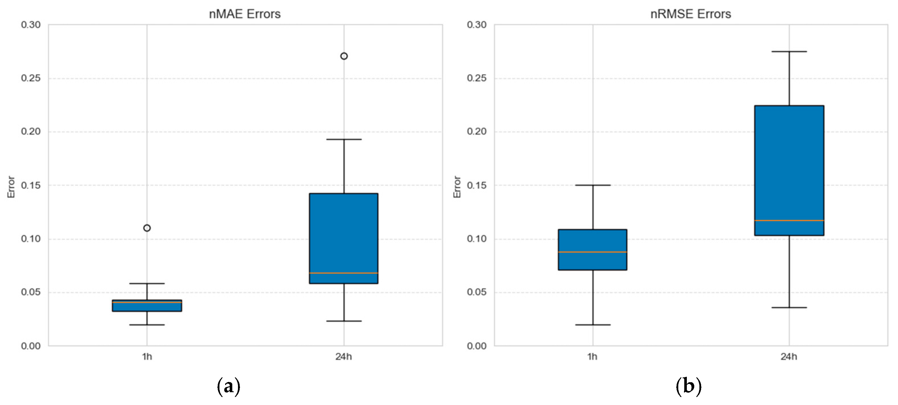
Forecast accuracy over a given time frame can be assessed in two ways, depending on the relationship between the “step” and “horizon” parameters. In the aggregate approach, a single forecast is produced for the entire period (e.g., total wind-generated energy over 24 h), and an error metric (such as RMSE or MAE) is applied to that aggregated value. As positive and negative deviations within the period can offset one another, this method often yields lower, potentially optimistic error estimates. In the sequential approach, the same horizon is divided into smaller intervals (e.g., 24 one-hour forecasts), each squared error is calculated, these nonnegative values are summed, and the appropriate root or average is taken.

Key performance indicators, such as normalized mean absolute error and normalized root mean squared error, were extracted from the literature [32,33,34,35,36,37,38,39,40,41,42,43,44,45,46,47,48,49,50,51,52] and visualized in Figure 1. It is evident that forecasting for a 24-h horizon (aggregate approach) presents higher errors than for a 1-h horizon, especially for nMAE and nRMSE values.

The forecasting step of 1 h (sequential approach, see

Table 1. nMAE and nRMSE errors from the literature analysis [32,33,34,35,36,37,38,39,40,41,42,43,44,45,46,47,48,49,50,51,52] for different forecasting steps.

Metrics	nMAE		nRMSE
Step	1 h	24 h	1 h	24 h
Mean	0.1042	0.0939	0.1405	-
Median	0.0803	0.0596	0.1089	-

) is also associated with higher errors, suggesting that capturing fine-grained variations in wind power generation remains challenging.

Analysis of forecasting methods’ performance metrics (see comparison of wind power forecasting models in Appendix A,

Table A1. Literature results analysis.

Model	Forecast Horizon	Forecast Step	Seasonality	Lags	nMAE	nRMSE	nMSE	sMAPE
Statistical Time Series Methods
sARIMA [32]	24 h	24 h	yes	yes, real	0.0596	-	0.081	-
sARIMA [32]	24 h	24 h	yes	yes, real	0.0619	-	0.0677	-
ARIMA [33]	1 h	1 h	no	yes, real	0.11	0.15	-	0.3771
SARIMA [34]	24 h	1 h	yes	yes, real	-	0.146	-	-
SARIMAX [35]	24 h	1 h	yes	yes, real	-	0.1222	-	-
Linear regression [36]	1 h	1 h	no	no	0.0433	0.1088	-	-
Markov chain model [37]	24 h	1 h	yes	no	0.062	0.714	-	-
Machine Learning Methods
LSTM-SMI [33]	1 h	1 h	no	yes, real	0.02	0.02	-	0.0913
XGBoost [33]	1 h	1 h	no	yes, real	-	-	-	0.1406
RNN [33]	1 h	1 h	no	yes, real	-	-	-	0.2727
GRU-MSI (Seasonal Mean Imputation) [33]	1 h	1 h	no	yes, real	-	-	-	0.0768
SVR (support vector regression) [38]	24 h	1 h	no	no	-	0.0821	-	-
ELM (extreme learning machines) [39]	24 h	1 h	no	no	-	0.0899	-	-
Linear SVR [36]	1 h	1 h	no	no	0.0414	0.1194	-	-
K Neighbors Regressor [36]	1 h	1 h	no	no	0.0291	0.0649	-	-
Decision tree regressor [36]	1 h	1 h	no	no	0.0397	0.0849	-	-
Gradient boosting [36]	1 h	1 h	no	no	0.0341	0.0726	-	-
XGBoost [36]	1 h	1 h	no	no	0.0261	0.0597	-	-
Random forest regressor [36]	1 h	1 h	no	no	0.0331	0.0847	-	-
LSTM [36]	1 h	1 h	no	no	0.0582	0.0901	-	-
Ridge [36]	1 h	1 h	no	no	0.0433	0.1088	-	-
Lasso [36]	1 h	1 h	no	no	0.0425	0.1066	-	-
ILSTM [40]	4 h	1 h	yes	yes, real	-	-	-	0.119
LSTM [40]	4 h	1 h	yes	yes, real	-	-	-	0.159
CNN-ALSTM-AR [41]	24 h	24 h	no	no	0.271	-	-	0.1687
LSMT [42]	24 h	1 h	yes	yes, real	-	0.2751	-	-
LSTM-WPRE [43]	24 h	?	yes	yes, real	-	0.112	-	0.094
Deep-LSTM [44]	24 h	1 h	no	yes	-	-	0.0079	-
Deep-GRU [44]	24 h	1 h	no	yes	-	-	0.0081	-
1D-CNN [44]	24 h	1 h	no	yes	-	-	0.017	-
Deep-LSTM [44]	24 h	1 h	no	yes	-	-	0.007	-
Deep-GRU [44]	24 h	1 h	no	yes	-	-	0.0074	-
1D-CNN [44]	24 h	1 h	no	yes	-	-	0.0197	-
nonlinear autoregressive NAR-NN [32]	24 h	24 h	yes	yes, real	0.0231	-	0.0304	-
nonlinear autoregressive NAR-NN [32]	24 h	24 h	yes	yes, real	0.0538	-	0.0515	-
Hybrid Strategies
Distance-weighted kernel density estimation (KDE) and regular vine (R-vine) copula [45]	24 h	1 h	no	yes, real	0.075	0.1089	-	-
Three-Step Hybrid Forecasting Method [46]	24 h	1 h	yes	yes, real	0.0803	0.102	-	-
Hybrid VMD-CNN-GRU-based model [47]	0.25 h	0.25 h	no	yes, real	-	-	-	0.1132
MRMLE-AMS—Multilearner Ensemble and Adaptive Model Selection [48]	18 h	6 h	no	yes, forecast	0.0943	0.1254	-	-
VMD-mRMR-FA-LSTM [49]	24 h	0.08 h	no	yes, forecast	0.0348	0.0358	-	-
Direct-VMD-LSTM [50]	24 h	1 h	no	yes, forecast	0.1287	0.107	-	-
VMD-BP [50]	24 h	1 h	no	yes, forecast	0.1927	0.1927	-	-
MDE Multi-distribution ensemble probabilistic wind power forecasting—ScienceDirect	24 h	?	no	?	0.1841	0.2355	-	-
LTC-NCP [44]	24 h	1 h	no	yes	-	-	0.0047	-
LTC-Fully-Connected [44]	24 h	1 h	no	yes	-	-	0.0048	-
CfC-NCP [44]	24 h	1 h	no	yes	-	-	0.004	-
CfC-Fully-Connected [44]	24 h	1 h	no	yes	-	-	0.0041	-
LTC-NCP [44]	24 h	1 h	no	yes	-	-	0.0062	-
LTC-Fully-Connected [44]	24 h	1 h	no	yes	-	-	0.0052	-
CfC-NCP [44]	24 h	1 h	no	yes	-	-	0.0051	-
CfC-Fully-Connected [44]	24 h	1 h	no	yes	-	-	0.0052	-
Hybrid (NWP-based)
Stacked physics-informed machine learning model [42]	24 h	1 h	yes	yes, real	-	0.2477	-	-
GBRBM-DBN consists of the PCA, NWP, and SC [51]	24 h	24 h	yes	yes, real	-	0.2173	-	-

) shows significant differences between different approaches. Statistical methods work well for stable conditions but struggle with rapid wind changes. Machine learning models, such as XGBoost and neural networks, perform better by capturing complex patterns and reducing errors. However, even these models have limitations, especially for short-term (24-h) forecasting and fine time (1-h) steps, where errors remain high.

Overall, analysis of the above studies indicates that hybrid forecasting approaches combining machine learning with dynamic time-series modeling are highly promising, with XGBoost and LTC models being the most promising ones. XGBoost is well-suited for selecting important features and handling structured data, but the model cannot track the changing behavior of the wind over time [21,25]. LTC, on the other hand, is better at capturing and adjusting to wind fluctuations than standard neural networks [29]. Therefore, a study investigating how combining XGBoost and LTC strengths could improve the accuracy of wind power forecasts (especially short-term with a 1-h time step) seems to be meaningful and relevant. Of course, an objective evaluation of the proposed idea requires a forecast accuracy comparison of the hybrid model with other alternative models, such as LSTM or a group of statistical models (e.g., Exponential Smoothing, ARIMAX, and Random Walk with Drift) under the same conditions.

The following chapters of this paper provide a comprehensive description of implemented research, focused on wind power forecast accuracy analysis of hybrid (XGBoost + LTC), XBoost, LTC, LSTM and statistical (i.e., Exponential Smoothing, ARIMAX, and Random Walk with Drift) models.

3. Dataset

The dataset was collected from an Enercon E82/2000 wind turbine (maximum generation capacity is 2000 kW) located in the Taurage region, in western Lithuania. Figure 2 shows that the Taurage region is formed by flat plains, with a few hills in the northern part. The average altitude is around 38 m above sea level.

The dataset represents a detailed time-series record of wind power generation and associated weather parameters collected in Lithuania. The dataset consists of 8760 records corresponding to hourly data collected throughout the year and is organized into 23 columns. Columns include both predicted values, such as weather forecasts, and factual measured values (data obtained from the Lithuanian Hydrometeorological Service), allowing a comparison between expected and real conditions. The factual values of measured meteorological data were calculated as the average of data from nearby automatic meteorological stations (Tauragė, Pagėgiai, Šilutė, Šilalė, Raseiniai, Jurbarkas). LHMT air temperature and wind element data are provided at 2 and 10 m above ground level, respectively.

Each dataset row corresponds to an hourly timestamp, capturing:

• Power generation: The factual power output (power_kw) is recorded, reflecting the efficiency and performance of the wind energy system.
• Predicted weather parameters: These include forecasted air temperature, cloud cover, feels-like temperature, relative humidity, sea-level pressure, total precipitation, wind direction, wind gust, and wind speed. Additionally, a condition code (e.g., “rain,” “heavy rain”) summarizes predicted weather.
• Factual weather measurements: These are factual weather conditions that were observed and recorded. They match the types of information found in the predicted data, making it possible to check how accurate the forecasts are. This includes real measurements of air temperature, cloud cover, wind speed, wind gusts, wind direction, total precipitation, and more.

The dataset is composed of both quantitative features, such as temperature, wind speed, and precipitation, and categorical features, such as weather condition codes, providing a diverse range of information for analysis.

4. Methodology

In this study, a structured and systematic methodology was employed to develop a predictive model for wind power generation. The goal was to balance model complexity, ensure robustness, and improve prediction accuracy. The methodology consists of multiple interconnected steps, including feature selection, feature engineering, and model development with an iterative optimization process (see Figure 3).

Each step of the methodology is discussed in more detail below.

4.1. Feature Selection

Although the initial dataset consisted of 23 columns, only 10 columns were selected for the final dataset. All columns of factual future values, such as factual temperature, have been removed, leaving predicted parameters and thus simulating a realistic scenario with no factual future observations. This has helped to reduce the complexity of the model by identifying and preserving only the most relevant features.

Given the structure of the dataset, which contains both categorical and quantitative features, the importance of features was assessed in two different ways, using the Random Forest ML algorithm and correlation analysis. Random Forest-based feature importance evaluation effectively captures non-linear relationships and handles categorical features, while correlation analysis provides insights into the linear relationships between numerical features and target variables.

4.1.1. Feature Importance Evaluation by Random Forest

Random Forest, a robust ensemble-based ML algorithm, measures feature importance based on how much each feature contributes to reducing impurity in the feature selection model. Such an approach is very practical when capturing non-linear data point relationships and non-linear interactions among the features [53].

To ensure enough data for both algorithm development and evaluation, each monthly dataset was split into training (70%), validation (15%), and testing (15%) subsets.

Once the training process was completed, the importance scores of the features were extracted to analyze the impact of each feature on model predictions. Feature importance was calculated based on the mean decrease in impurity (MDI), also referred to as Gini importance. Specifically, the importance of a feature is determined as an average reduction in node impurity contributed by that feature across all decision trees within the ensemble. Impurity reduction is weighted by the number of samples reaching each node and then averaged across the forest [54].

Random Forest algorithm-based calculations (see

Table 2. The most influential features for the power_kw variable based on the Random Forest Regressor model.

Feature	Gini Importance Score
predict_wind_speed	0.511286
predict_wind_direction	0.083863
predict_wind	0.074096
predict_sea_level_pressure	0.065375
predict_relative_humidity	0.063730
predict_air_temperature	0.063255
predict_feels_like_temperature	0.061680
predict_cloud_cover	0.037996
predict_wind_gust	0.029197
predict_total_precipitation	0.009522

) showed that four most influential parameters for power_kw variable are predicted: wind speed (predict_wind_speed), predicted wind direction (predict_wind_direction), predicted wind (predict_wind, defined as the sum of predicted wind speed and predicted wind gust), and predicted sea level pressure (predict_sea_level_pressure).

4.1.2. Feature Importance Evaluation by Pearson Correlation Coefficients

As an alternative approach to identifying influential features, Pearson correlation coefficients were computed between the features and the target variable power_kw. Such analysis can be concluded with a correlation matrix, which gives information about interpreting relationships between all predictor variables and the target variable. High correlation values indicate that features are strongly related either positively or negatively and can be prioritized for research [55].

The results (see

Table 3. The most influential features for the power_kw variable based on correlation analysis.

Feature	Correlation Coefficient
predict_wind_speed	0.751703
predict_wind	0.739799
predict_wind_gust	0.719605
predict_sea_level_pressure	0.350786
predict_feels_like_temperature	0.200739
predict_air_temperature	0.174140
predict_relative_humidity	0.158937
predict_cloud_cover	0.125714
predict_wind_direction	0.120283
predict_total_precipitation	0.113998

) confirmed the importance of three features: predict_wind, predict_wind_speed, and predict_sea_level_pressure, as well as identified an additional highly influential feature related to the strength of wind gusts (predict_wind_gust).

The final selection of features was based on identifying predictors that appeared in both the Random Forest feature importance and Pearson correlation analysis lists, ensuring consistency across the methods. This overlap highlights features deemed influential by both linear and non-linear evaluation approaches, resulting in a robust and reliable selection. Based on the findings, further work was conducted using predict_wind_speed, predict_wind, predict_wind_gust, predict_wind_direction, and predict_sea_level_pressure parameters.

4.2. Feature Engineering

To create a robust and stable model, the following features were added to the dataset:

• Time-based features: attributes such as month were extracted to capture seasonal variations in wind power generation. Each month has its own wind speed trend, with distinct patterns that reflect the influence of seasonal changes, such as higher wind speeds in winter months and lower wind speeds in summer. Including these monthly trends helps the model account for the natural fluctuations in wind power generation throughout the year [56].
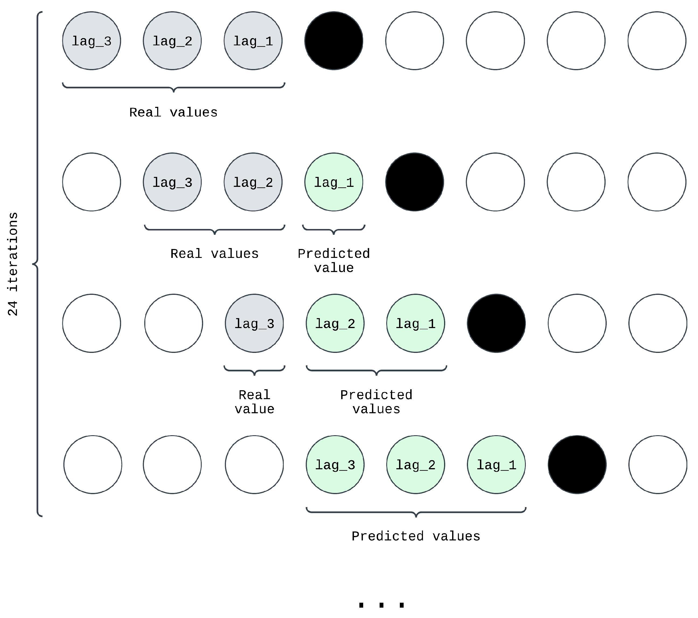
• Lag features: wind power values from previous time intervals (lags of 1, 2, and 3 steps) were included. These lagged features provide a way to model the natural dependence of wind power on past values. Initially, these were populated using factual historical data [57].

4.3. Model Development Process

Each model had to pass the modeling process, consisting of the following steps:

• Initial training: The model was trained on the dataset where lag features were based on factual historical values.
• Hyperparameter optimization: To improve performance, Bayesian optimization was used to fine-tune the model’s parameters. This included optimizing the number of estimators, maximum depth, learning rate, and minimum child weight. The goal was to minimize the Mean Absolute Error (MAE) on the validation dataset.
• Iterative training with predictions: after initial training, lag features were updated using model predictions rather than factual values (see Figure 4). This step mimics real-world scenarios where predictions depend on prior forecasts. The model was retrained with these updated lag features to enhance its ability to handle sequential dependencies.

4.4. Aspects of the Development of Selected Models

After selecting and engineering the relevant features, XGBoost, LTC, LSTM, and Hybrid models were developed. All four models were refined through Bayesian hyperparameter and architecture tuning to minimize mean squared error (MSE) loss (see Section 4.3 for details). During hyperparameter search and training, each model used a different set of lags (see

Table 4. Lag Specifications for XGBoost, LTC, and Hybrid Models.

Model	Lags
XGBoost	generated power values of past 1–3 h (lags)
LTC	generated power values of 3rd, 5th, 7th, 8th, 11th, 13th, 15th, 16th, 17th, 18th, 19th, 22nd, and 24th lags
LSTM	generated power values of 1st, 4th, 9th, 11th, 12th, 13th, 15th, 17th, 21st, 23rd, and 24th lags
Hybrid (XGBoost + LTC)	-

).

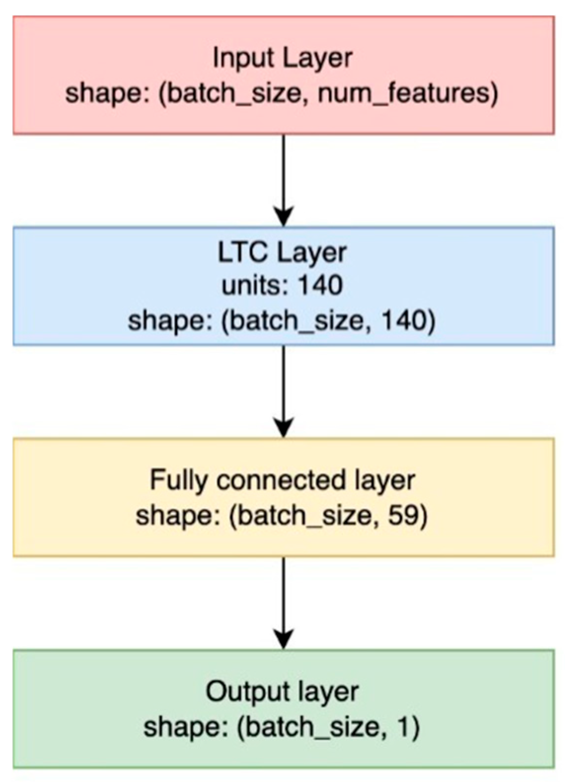
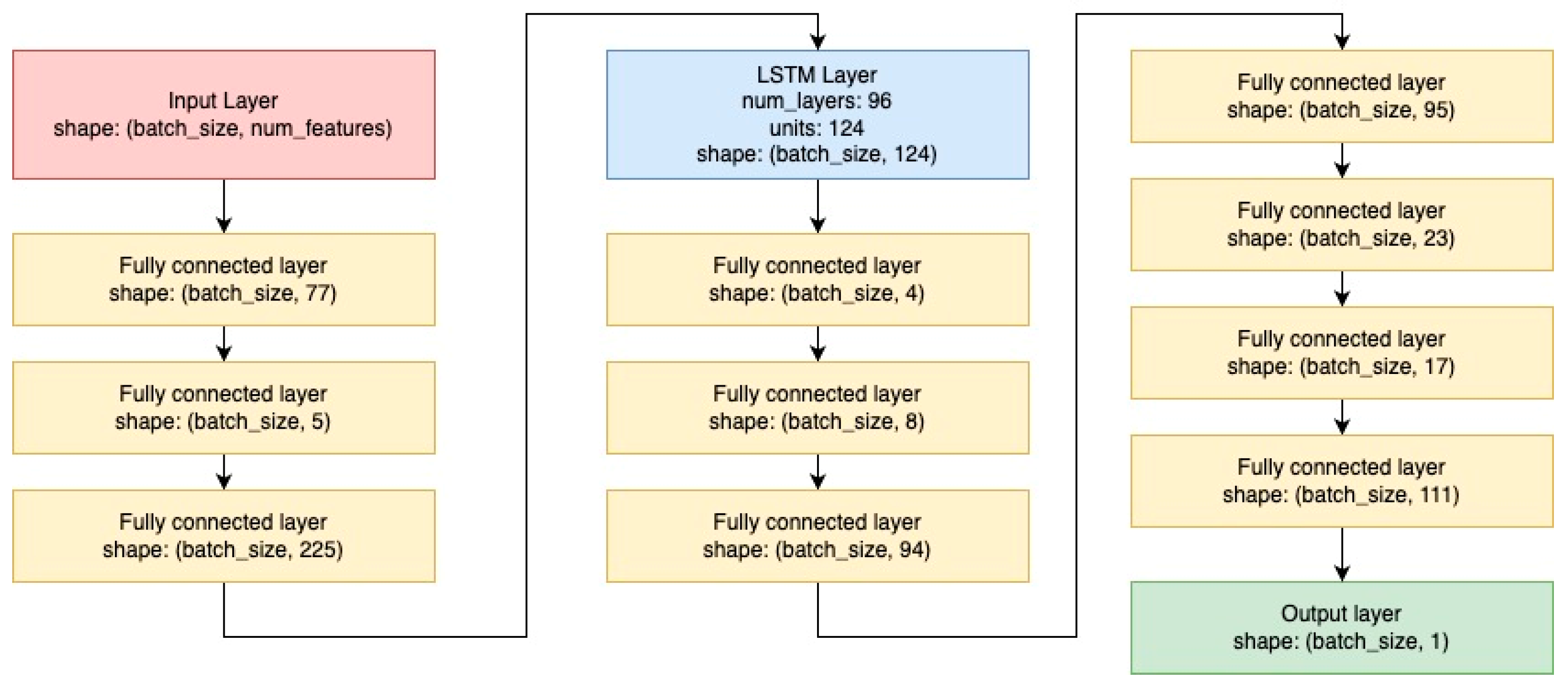
LTC as well as LSTM layers were wrapped by additional layers of a fully connected neural network. For the LTC model, the fully connected layer with a tanh activation function, accompanied by a dropout rate of 20% was used. In both models, the output layer is composed of a single neuron. The final LTC and LSTM architectures are presented in Figure 5 and Figure 6. The best results for the XGBoost model were achieved using a Bayesian optimizer, which aimed to minimize the Mean Squared Error (MSE) by identifying optimal parameters within the following ranges: number of estimators [100, 500], learning rate [0.01, 0.3], maximum depth [3, 10], and minimum child weight [0.1, 10]. The resulting best parameters were: learning rate: 0.055, maximum depth: 4, minimum child weight: 1.522, and number of estimators: 266.

XGBoost and Hybrid models were trained using K-Fold cross-validation, a technique that contributed to improved model performance. This method enhances the robustness of training by reducing the likelihood of overfitting to specific subsets of the data. As a result, models trained with K-Fold cross-validation are better equipped to generalize to unseen data, leading to more reliable and accurate predictions.

Statistical models RWD, ETS, and ARIMAX were trained without a Bayesian optimization step, while ARIMAX passed a multicollinearity check. The predict_wind parameter showed the highest variance-inflation factor and was therefore removed prior to model fitting. Also, to improve the forecast, in all models, the lagged values method (using up to three previous steps) was used.

Finally, in the Hybrid model (see Figure 7), to combine XGBoost and LTC, a multi-layer perceptron regressor (MLP regressor) was chosen. The MLP Regressor is used to predict wind-generated power values based on several input features, such as predicted outputs from XGBoost and LTC models, along with the predicted wind speed and wind gust.

The MLP network has three hidden layers, with the data features for this model selected manually by testing the accuracy with different feature combinations. The number of neurons and other hyperparameters was chosen using Bayesian optimization.

4.5. Metrics for Assessing Models’ Accuracy

To measure the accuracy of the models, Mean Absolute Error (MAE) and Root Mean Squared Error (RMSE) metrics were used. MAE measures the average absolute differences between predicted values (y′_i) and the factual values (y_i) over n observations and is mathematically expressed as shown in Equation (1):

$$MAE ={\displaystyle \frac{1}{n}}{\sum }_{i=1}^n\left|y_i-y_i^{\prime }\right|$$

(1)

RMSE is defined as the square root of average of squared errors [52]. This metric is widely used because it amplifies the impact of larger errors while deemphasizing smaller ones. The RMSE is mathematically expressed as shown in Equation (2):

$$RMSE =\sqrt{{\displaystyle \frac{1}{n}}{\sum }_{i=1}^n{\left(y_i-y_i^{\prime }\right)}^2}$$

(2)

These metrics were chosen as they are widely used in wind power prediction and provide complementary insights into model performance. MAE indicates the average prediction error, while RMSE, due to its squared error component, is more sensitive to the outliers.

In addition to the conventional metrics, normalized error metrics nMAE and nRMSE were computed as well. The normalized metrics are useful for facilitating scale-independent comparisons across different systems or scenarios and are mathematically expressed as shown in Equations (3) and (4):

$$nMAE = {\displaystyle \frac{MAE}{N_{max}}}={\displaystyle \frac{1}{N_{max}}}\cdot {\displaystyle \frac{1}{n}}{\sum }_{i=1}^n\left|y_i-y_i^{\prime }\right|$$

(3)

$$nRMSE ={\displaystyle \frac{RMSE}{N_{max}}}={\displaystyle \frac{1}{N_{max}}}\sqrt{{\displaystyle \frac{1}{n}}{\sum }_{i=1}^n{\left(y_i-y_i^{\prime }\right)}^2}$$

(4)

where N_max represents the maximum generated power, which is equal to 2000 kW in this study.

5. Results

The aim of the first experiment was to compare and evaluate the accuracy of wind power predictions produced by the respective model architectures described in Section 4. The study evaluated the resulting forecast errors and training time to determine which models are not only accurate but also efficient.

Table 5. Experimental (n)MAE and (n)RMSE values describing wind power prediction accuracy of analyzed models.

Model	nMAE	nRMSE	MAE	RMSE	Training Duration (s)
LSTM	0.2119	0.2437	423.8	487.4	16,250.4
Exponential Smoothing	0.1059	0.1345	211.8	269.0	41.56
ARIMAX	0.1052	0.1336	210.4	267.2	52.54
Random Walk with Drift	0.1046	0.1331	209.2	266.2	35.39
LTC	0.1020	0.1264	204.0	252.8	695.0
XGBoost	0.1052	0.1258	210.4	251.6	57.6
Hybrid (XGBoost + LTC)	0.0856	0.1092	171.2	218.4	30.8 (783.4) 1

¹ With XGBoost and the LTC model’s training took 783.4 s.

shows the resulting values of MAE and RMSE metrics (both reported and normalized) describing the accuracy of the models, as well as the time taken to train them.

LSTM model, as shown in the first row of Table 5, presented a weak correlation between wind speed, wind gusts and generated power, providing not only the poorest (nMAE = 0.2119, nRMSE = 0.2437) wind power prediction results, but also requiring an extremely long time (16,250.4 s) to train. This duration was at least 27 times longer than that of any other model evaluated in the experiment. This indicates that this model is less suitable for wind power forecasting when wind behavior is particularly erratic or when the data is noisy. These findings are supported by results obtained by other researchers, which show that the model performs reasonably well for a short period of 1-h forecasts, but the accuracy of the model’s prediction decreases significantly for longer periods (e.g., when the forecast horizon is 24 h) [14].

Statistical methods, including Exponential Smoothing, ARIMAX, and Random Walk with Drift (see gray shaded rows in Table 5), demonstrate significantly better performance and efficiency than the LSTM model. All three methods yielded similar results in (n)MAE and (n)RMSE metrics, which indicates that time series patterns are captured well by all of them. However, the Random Walk with Drift model took the shortest time (35.39 s) to train compared to the other two models; thus, from the accuracy and training time perspective, it could be considered the most efficient in the group.

Moving back to machine learning models, the LTC model outperformed LSTM, XGBoost, and statistical methods by at least ~2% in terms of MAE error metrics, which proves its potential in wind power prediction. At least 5% better RMSE values show that LTC, as well as XGBoost, handle outliers better. Despite the computational complexity of neural networks, which was more time-consuming than statistical methods, the potential of both methods for wind power prediction is clearly evident.

The Hybrid (XGBoost + LTC) model achieved the best overall performance, balancing accuracy and efficiency. Compared to the best-performing models, its MAE and RMSE values improved by at least 16% and 13% respectively, keeping the model’s training time relatively low. This suggests that hybrid models, leveraging the strengths of machine learning methods, can offer the best trade-off between accuracy and computational cost.

Given the best results obtained with LTC, XGBoost, and Hybrid (XGBoost + LTC) models, further in-depth studies were limited to this group.

5.1. Application of Filtering to Predicted Values

The study was carried out to assess the impact of wind speed and gusts on LTC, XGBoost, and Hybrid models’ predictions with respect to wind turbine characteristics. It is important since if the wind speed is too low, there is not enough energy to turn on the generator. If the wind is too strong, it can cause some damage, and the generator must be shut down. The power curve of the Enercon E82/2000 wind turbine in Figure 8 shows that the minimum wind speed required to start the turbine is 2 m/s, and the turbine is stopped at wind speeds above 25.5 m/s. The maximum generated power is reached at a wind speed of 12.5 m/s.

The experiment tested whether wind speed falls within the range of the wind turbine power curve and whether wind speed, together with wind gusts, remains within the range. In this context, LTC, XGBoost, and Hybrid forecast values were filtered and predictions adjusted (see

Table 6. Comparison of the errors with and without prediction filtering.

	Filtered Wind Speed		Filtered Wind Speed + Wind Gust		Unfiltered
Models	nMAE	nRMSE	nMAE	nRMSE	nMAE	nRMSE
XGBoost	0.0943	0.1329	0.0998	0.1352	0.1052	0.1258
LTC	0.0948	0.1394	0.0980	0.1406	0.1020	0.1264
Hybrid	0.0800	0.1210	0.0828	0.1221	0.0856	0.1092

). When filtering by wind speed, nMAE errors decreased across all models by ~6.5–10%, while nRMSE increased by ~6–10%.

This shows that filtering worked as a trade-off between nMAE and nRMSE errors. While the predictions improved on average, they worsened in extreme cases. Filtering by wind speed and wind gust reduced nMAE errors only by ~3–5%, while nRMSE errors increased by ~7–12%. This also shows that additional filtering smooths variations but does not improve overall performance, as it may introduce new biases or amplify large errors.

5.2. Models’ Adaptation to Wind Speed and Wind Gust Fluctuations

The experiment investigated how time intervals with different wind speed patterns can impact models’ accuracy.

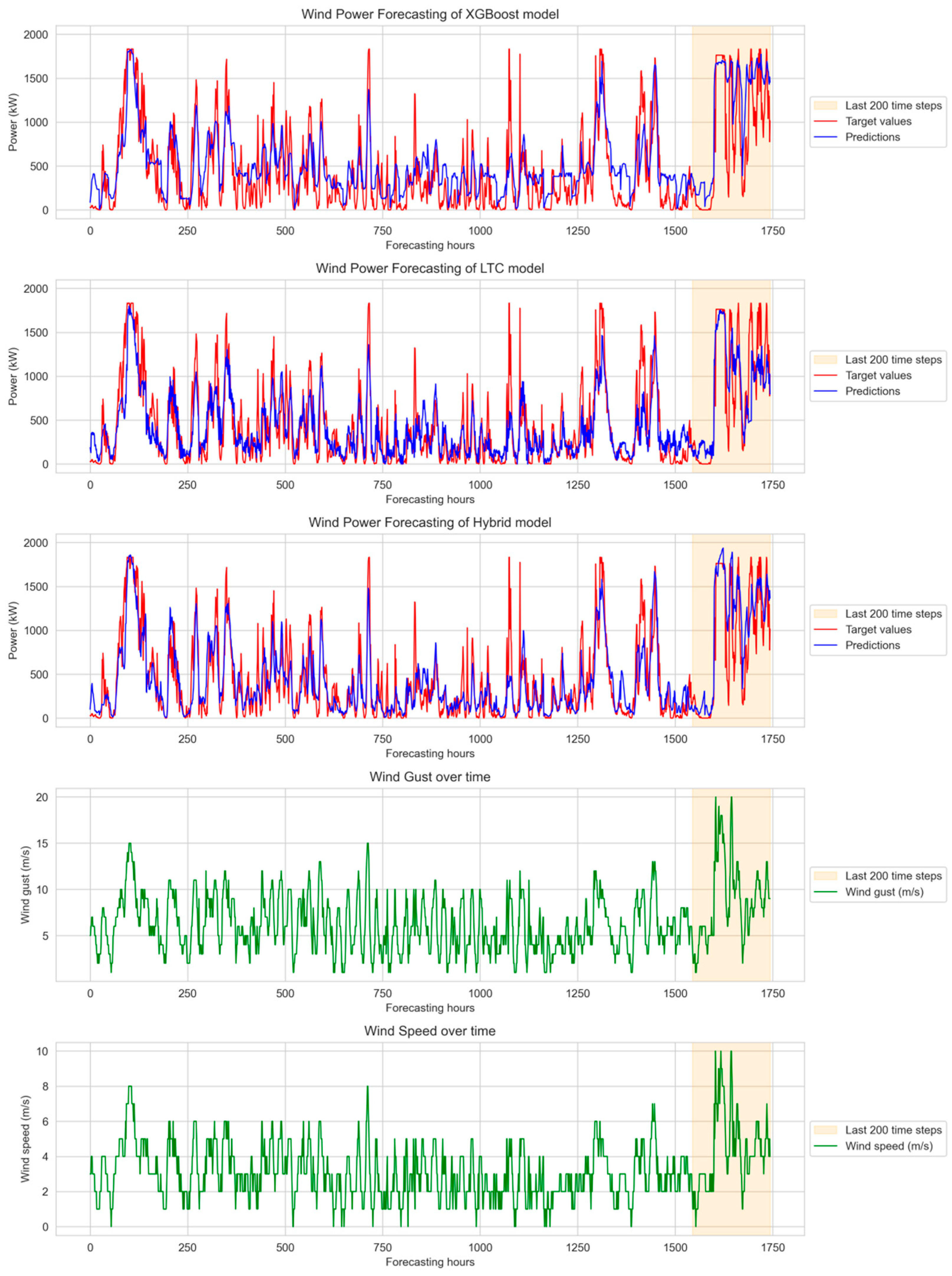
XGBoost, LTC and Hybrid models’ forecasting results together with input wind gust and wind speed features show XGBoost and LTC models’ strong ability to adapt to changes in the target values, but both models struggle to accurately capture extreme peaks, which leads to significant deviations (see areas highlighted with yellow in Figure 9). At the end of the year, wind gusts and wind speeds were unprecedentedly high, which contributed to larger fluctuations in predicted values. The hybrid model, however, demonstrates that its predictions are always within the target values. Although there are still extreme cases, the model captures fluctuations more effectively than XGBoost or LTC.

As the beginning and the end of the time series show different fluctuations and variance in input data and predictions, the first and last 200 steps of the forecast, along with wind speed and gust, were analyzed in more detail.

Table 7. Error comparison of the first and last 200-time steps series periods.

	nMAE			nRMSE
Models	XGBoost	LTC	Hybrid	XGBoost	LTC	Hybrid
First period	0.10028	0.10085	0.07762	0.13132	0.13869	0.11518
Last period	0.16364	0.13169	0.12671	0.21854	0.18778	0.17142

shows the Hybrid model’s overall accuracy advantage over XBoost and LTC models in the first and last 200-time steps (MAE = 0.07762 in the first 200-time steps and MAE = 0.12671 in the last 200-time steps). These results confirm the Hybrid model’s ability to adapt more effectively to different weather conditions and its instability compared to XGBoost and LTC models.

Additionally, the bigger first and last periods’ nMAE error difference for both XGBoost and Hybrid models indicates that, during periods of high wind speed and gust fluctuations, Hybrid and XGBoost are less effective than LTC. However, over the long term, during calmer periods, Hybrid and XGBoost models demonstrate greater efficiency than the LTC model alone.

The difference in nRMSE values in calm and high wind speed periods indicates that the Hybrid model handles outliers better than XGBoost but not as well as LTC.

5.3. Analysis of Models’ Features

In addition to the model’s accuracy characteristic, the stability feature is equally important. Stability ensures that the model performs consistently over time, avoiding fluctuations, which can reduce trust in its reliability.

Evaluation of the stability aspect was carried out in three different ways: analyzing model MAE and RMSE values for short-term (24 h) and long-term (72 h) forecasts, as well as assessing the model’s prediction performance in different seasons.

Assessing model performance at the daily level reduces the impact of short-term fluctuations and biases in hourly data. The choice of daily (24 h) and three-day (72 h) hourly frequencies provides a standardized and consistent time interval, which is commonly used in the NordPool market. Furthermore, NordPool allows participants to trade electricity across multiple European countries through a centralized, transparent platform. Power generation companies are required to submit day-ahead price forecasts. However, in practice, these forecasts are typically made 2–3 days in advance, optimally 72 h, and are subsequently adjusted daily based on new predictions. Models’ performance across seasons displays their ability to adapt to different weather fluctuations, since each season has specific weather patterns. Long-term observations of meteorological elements, including wind speed values and their fluctuations, in Lithuania showed that the strongest and most gusty winds are observed in January, November, and December [58].

For all 3 experiments, the full dataset of 8760 h was used. This solution was chosen to keep time intervals within complex forecasting conditions. Also, using a full dataset ensures the continuity of the 72-h sequence, which would otherwise be compromised.

For the second model stability experiment (Section 5.3.2), the entire dataset was split into 3 parts—training, validation, and test datasets. The training dataset contained 220 days (5280 h), and the validation and testing datasets contained 72 days (1728 h) of information. Errors in validation and test datasets reveal the model’s ability to perform on unseen data.

5.3.1. Models’ Accuracy and Stability by Daily Error Metrics

Calculation of daily performance measures like nMAE and nRMSE enables meaningful comparison of model predictions. The average error reflects the overall model performance, whereas the median error provides the typical error, indicating model robustness and outlier resistance. A stronger model has lower error variance and a consistent mean and median over multiple days, as it can generalize well across various wind conditions and reduce deviations from factual power generation.

In

Table 8. Models’ mean and median errors comparison.

	Mean		Median
Model	nRMSE	nMAE	nRMSE	nMAE
XGBoost	0.1258	0.1052	0.1180	0.0975
LTC	0.1264	0.1020	0.1134	0.0898
Hybrid	0.1092	0.0856	0.1003	0.0766

, it is visible that the Hybrid model outperforms all other models in both nMAE and nRMSE metrics with mean and median averaging. The hybrid model has a 15% lower mean nRMSE and 23% lower nMAE than the XGBoost model and a 16% lower mean nRMSE and 19% lower nMAE than the LTC model. The median of errors also decreased. The median nRMSE decreased by 18% in the Hybrid model compared to XGBoost, while the median nMAE decreased by 28%. Compared to LTC, the Hybrid model performed 13% better in median nRMSE metrics and 17% better in median nMAE. This indicates that the Hybrid model demonstrates superior performance and accuracy in both metrics, making it the most accurate model among the evaluated models on a daily level.

It can also be seen that consistently lower-than-average median errors indicate that there are large outliers that have a significant impact on the mean. However, most forecasts remain more accurate.

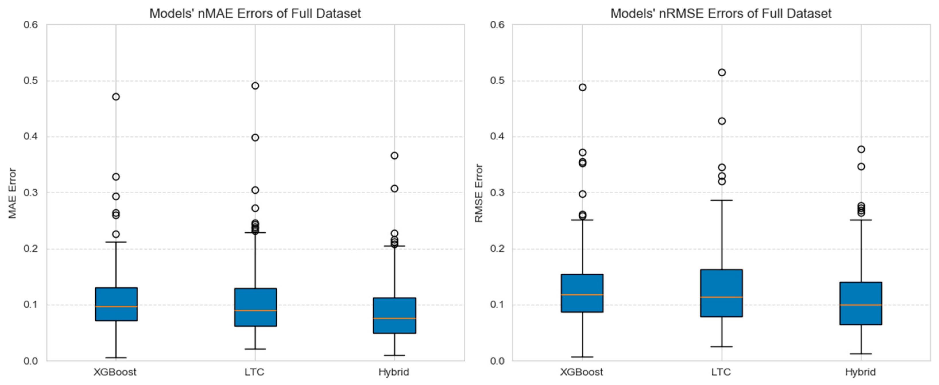
Figure 10 confirms these findings. It shows that all models contain several outliers. And they are visible in the previously mentioned Figure 9, the last 200-time-step interval.

Table 9. Comparison of models’ errors with different dataset subsets.

		Mean		Median
Model	Dataset Subset	nRMSE	nMAE	nRMSE	nMAE
XGBoost	train	0.119563	0.100066	0.115383	0.094826
	valid	0.134442	0.111880	0.112520	0.090439
	test	0.136202	0.114137	0.129338	0.104207
LTC	train	0.126650	0.102723	0.116041	0.094694
	valid	0.131850	0.106755	0.114850	0.087305
	test	0.120256	0.094945	0.106754	0.083323
Hybrid	train	0.105791	0.083193	0.100172	0.077115
	valid	0.117254	0.091856	0.102692	0.079701
	test	0.111630	0.086475	0.098890	0.073081

and Figure 11 show the comparison of errors across models and different data subsets. It is visible that XGBoost model validation and test dataset errors increased by ~14% in both nRMSE and nMAE metrics. This indicates that XGBoost does not generalize well to unseen data. On the other hand, the test data subset errors of the LTC model, compared to the training dataset errors, decreased by ~5% in nRMSE and ~8% in nMAE.

LTC model shows improved generalization, which indicates that the model might be more stable, resistant to overfitting, and effective at capturing general patterns in the dataset. The hybrid model falls between the XGBoost and LTC models. Its errors increase slightly during the test stage (nRMSE increases by 5.5% and nMAE by 4%) but remain lower than the XGBoost model. Even after such an increase, the error rate of the model remains low.

5.3.2. Models’ Performance in Seasons

Analyzing weather seasonality is crucial for understanding the accuracy of power generation forecasting across months and seasons. While summer tends to have calmer weather changes, winter has harsher and more volatile weather changes. The seasonality test allows us to see if these wind volatility changes affect the models’ robustness, accuracy, and reliability.

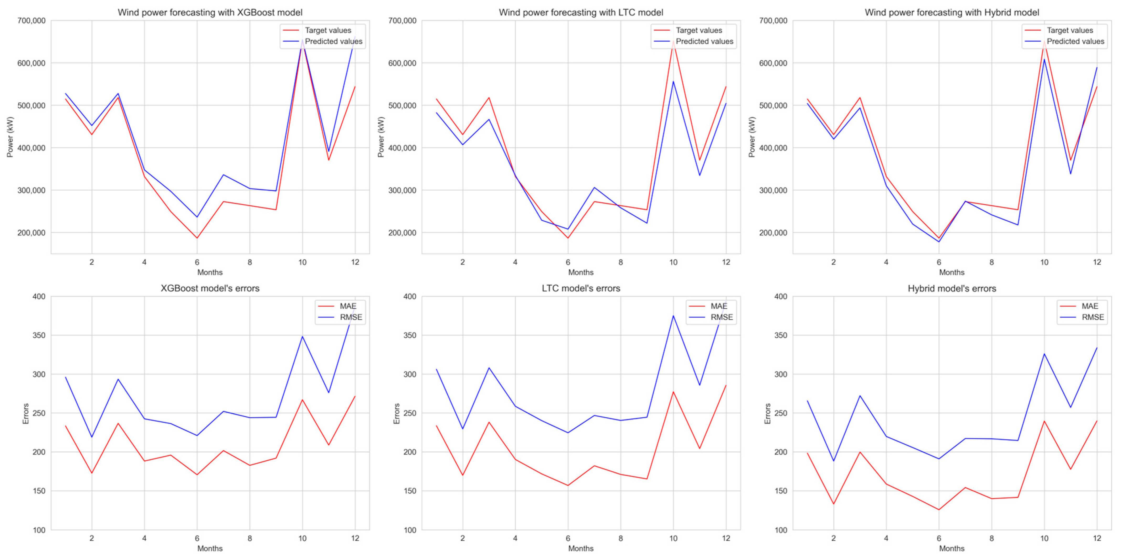
Figure 12 shows that the highest concentration of errors occurred in October and December, while June showed the fewest errors across all models. The largest difference between the lowest and highest errors is observed in the LTC model, while the smallest difference is observed in the Hybrid model. This displays the Hybrid model’s ability to better predict weather across all months. Additionally, a correlation has been observed between power generation and error rate, indicating that errors increase with higher power generation and vice versa.

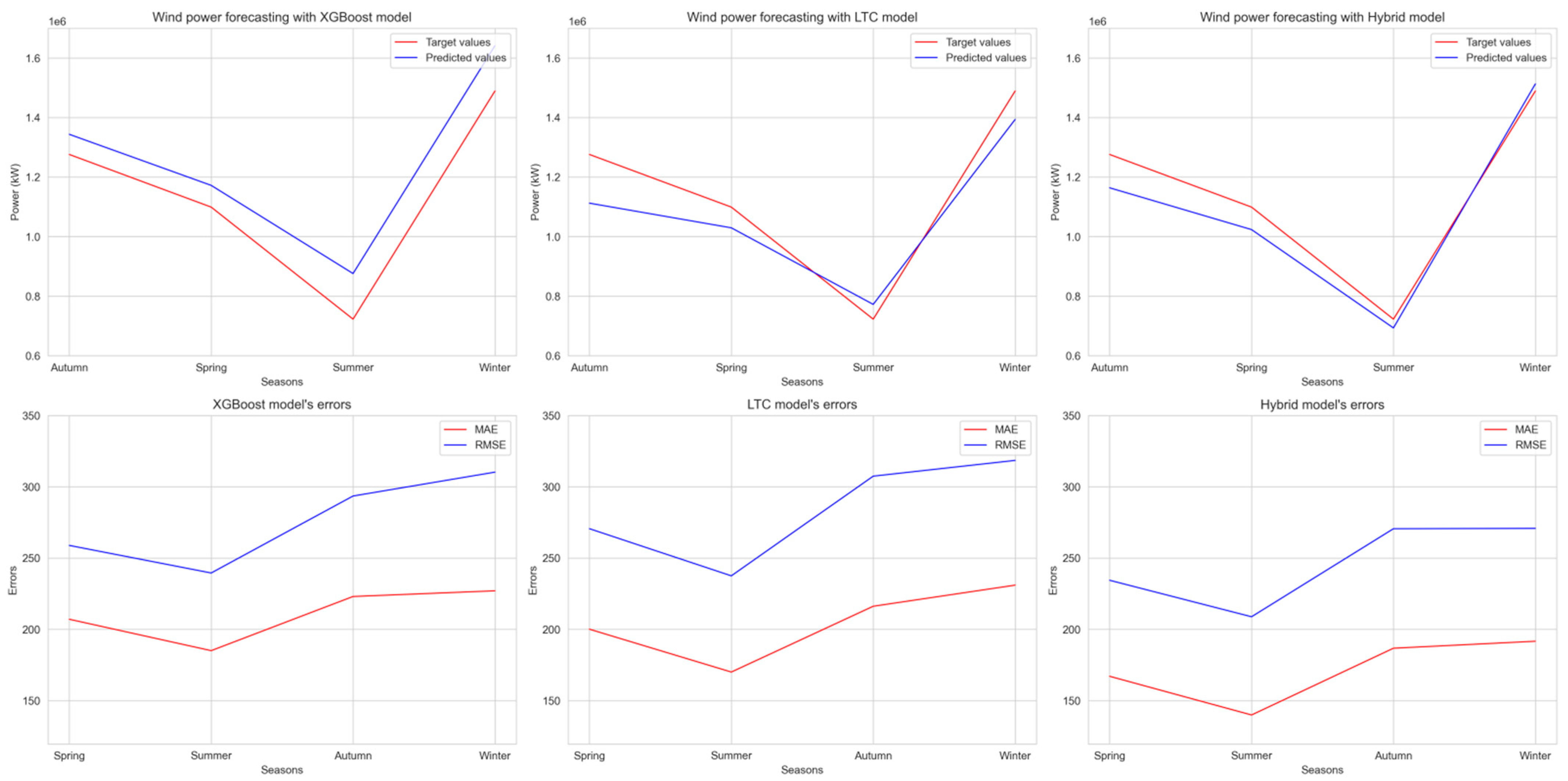
Figure 13 shows that in summer, all models have the best forecast accuracy, while in autumn and winter, forecast accuracy is the worst. The MAE and RMSE error graphs show that autumn and winter error rates are almost similar. The hybrid model is robust to different seasonal conditions, making it more accurate in all four seasons.

5.3.3. Evaluating Model Performance in Continuous 72-h Wind Power Forecasting

The performance of continuous wind power forecasting is important due to the accumulation of errors over time. A model’s ability to continuously predict all 72 h demonstrates its stability in handling long-term data, assuring reliable long-term predictions.

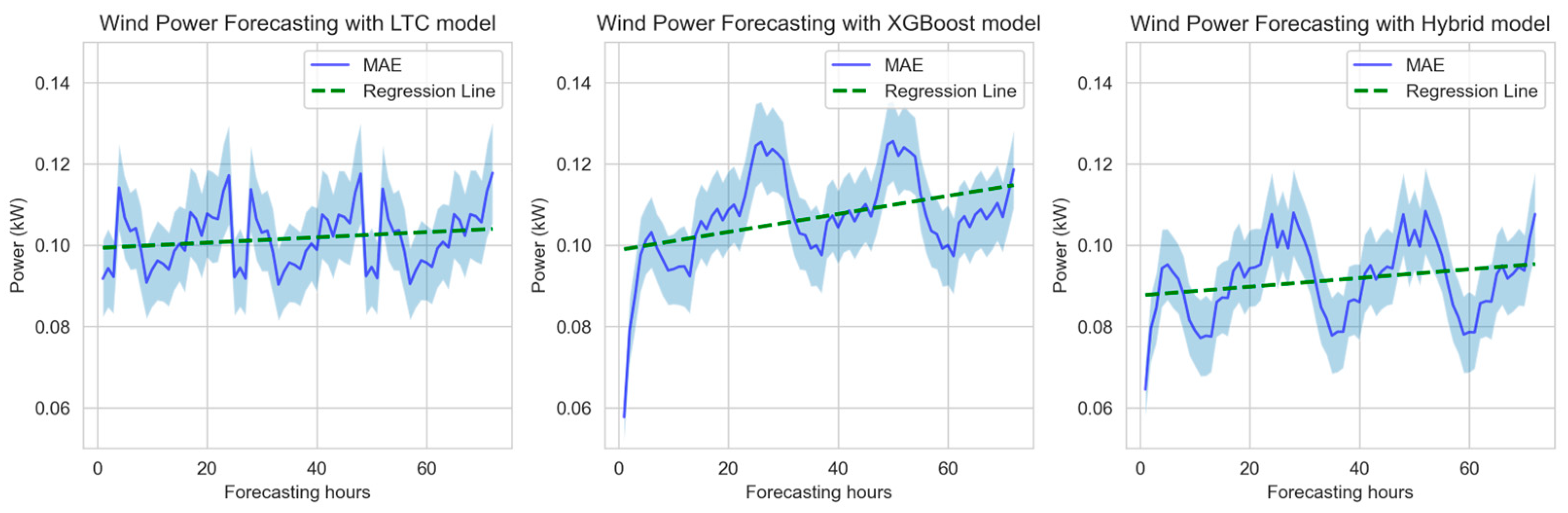
Figure 14 shows the hourly MAE change for XGBoost, LTC, and Hybrid models. XGBoost and Hybrid models have the lowest error in the first 3 h, while the LTC model displays consistent errors across all 72 h. This highlights models’ ability to consistently forecast wind power and makes LTC more reliable than other models in long-term wind forecasting. However, the Hybrid model consistently maintains the lowest errors throughout all hours, reinforcing its superior forecasting accuracy and robustness.

Figure 15 shows the MAE error with its confidence range, as well as its regression. LTC model has a consistent regression slope, whereas XGBoost exhibits a steeper slope. The hybrid model’s regression slope is 64% steeper than the LTC model’s regression slope, but 52% shallower than the XGBoost model’s regression slope. However, the hybrid model has a 12% initial error.

Confidence ranges further indicate that the LTC model maintains a stable error range over time, while both XGBoost and Hybrid models display an initial error with an almost negligible confidence range. This indicates that the LTC model is the most stable and reliable for long-term predictions, while the Hybrid model serves as a balanced compromise, offering a tradeoff between initial error and long-term error stability.

5.4. Comprehensive Economic Error Analysis

The errors in wind power forecasts have a great impact from an economic perspective. Larger and more frequent errors result in greater income losses. There are a few types of economic impact estimations: income that will not be received due to insufficient energy supply to the Nord Pool market exchange, and the penalties for undelivered energy. The aspects of these calculations are explained in more detail below.

During 2023, the wind turbine Enercon E82/2000 generated 4,587,000.43 kWh or 4587.00 MWh of energy. XGBoost predicted a total energy generation of 5,033,260.61 kWh (5033.26 MWh), which is 10% more than the factual energy generated. The LTC model predicted 4,307,797.35 kWh (4307.79 MWh) of energy, i.e., 6% less than the actual generation. The Hybrid model also predicted 4.2% less energy than the total amount of energy generated (4,393,924.05 kWh or 4393.92 MWh). These results indicate potential financial losses, as overestimations may lead to penalties for undelivered energy (e.g., XGBoost) and lost revenue due to underestimations (e.g., LTC and Hybrid models).

From

Table 10. The number of overestimated and underestimated hours resulting from the prediction of XGBoost, LTC, and Hybrid models.

	XGBoost	LTC	Hybrid
Overestimations in hours	5544 h	4655 h	4435 h
Underestimations in hours	3168 h	4054 h	4277 h
Exact estimations in hours	0 h	3 h	0 h

, it is visible that the XGBoost model overestimates more than it underestimates, while the LTC and Hybrid models do the opposite.

Earlier discussed over- and under-estimations in hours can be compared from a power perspective (see

Table 11. Calculated total amount of overestimated and underestimated energy resulting from the prediction of XGBoost, LTC, and Hybrid models.

	XGBoost	LTC	Hybrid
Overestimations (MWh)	1139	749	649
Underestimations (MWh)	693	1028	842

). The hybrid model overestimates 75.6% less power than the XGBoost model, but only 15.5% less compared to the LTC model. Additionally, the Hybrid model underestimates 17.6% more power than the XGBoost model, but 22% less than the LTC model. The hybrid model significantly reduces overestimation compared to XGBoost and underestimation compared to LTC, making it a more balanced and accurate power estimation model overall.

For both overestimation and underestimation calculations, the Nord Pool day-ahead hourly prices of Lithuania in 2023 were used. The total potential earnings were calculated by multiplying the factual electricity produced by the Nord Pool day-ahead prices (see Equation (5)), which resulted in a total amount of EUR 356,619.63.

$$\sum PotentialEarnings={\sum }_{i=1}^n{GP}_i\times {NPHP}_i$$

(5)

where: GP—Generated Power, NPHP—Nord Pool Hour Price.

To calculate the economic impact (penalties) of overestimations, we need to identify the days when overestimation occurred and multiply those days by the Nord Pool day-ahead price for that day (see Equation (6)):

$$\sum Penalty={\sum }_{i=1}^n\left\{\begin{array}{cc}\left(P{P}_i-{GP}_i\right)\times {NPHP}_i,& ifP{P}_i>{GP}_i\\ \hfill 0,& otherwise\hfill \end{array}\right.$$

(6)

where: PP—Predicted Power, GP—Generated Power, NPHP—Nord Pool Hour Price.

Table 12. Penalties comparison across XGBoost, LTC, and Hybrid models.

Model	Penalties (Eur in Thousands)	Percentage of Potential Earnings (%)	Earnings After Penalties (EUR in Thousands)
XGBoost	113	31.56	244
LTC	73	20.36	284
Hybrid	57	15.87	300

shows the penalties for the model’s underestimation. The Hybrid model generated 49.69% fewer penalties than the XGBoost model and 22.05% fewer penalties than the LTC model, demonstrating its superiority in terms of reducing penalty costs.

Another economic aspect that should be considered is the extra revenue loss. It happens when the model underestimates power generation, leading to missed opportunities to sell energy. Extra revenue is calculated by summing the differences between factual generated power and predicted power, multiplied by Nord Pool price, only in cases where factual generated power exceeds the predicted power (see Equation (7)):

$$\sum ExtraRevenueLoss={\sum }_{i=1}^n\left\{\begin{array}{cc}\left({GP}_i-P{P}_i\right)\times {NPHP}_i,& if{GP}_i>P{P}_i\\ \hfill 0,& otherwise\hfill \end{array}\right.$$

(7)

where: PP—Predicted Power, GP—Generated Power, NPHP—Nord Pool Hour Price

Extra revenue losses (see

Table 13. Extra revenue loss comparison across XGBoost, LTC, and Hybrid models.

Model	Extra Revenue Loss (Eur in Thousands)	Percentage of Potential Earnings (%)	Earnings After Extra Revenue Loss (Eur in Thousands)
XGBoost	56	15.61	301
LTC	83	23.34	273
Hybrid	74	20.87	282

) indicate that the least revenue is lost according to the XGBoost model results, while the LTC model underestimated the most, leading to an extra revenue loss of 83,251.19 EUR. The hybrid model incurs a revenue loss of 74,431.06 EUR, positioning it between XGBoost and LTC models in terms of performance. This is connected to the previous calculations (see Table 11), since the XGBoost model had the largest overestimation but the smallest underestimation. On the other hand, the LTC model had the largest additional revenue loss, even though it underestimated power generation at a medium rate (in between XGBoost and Hybrid) based on the number of days. This was because of the undervaluation of the LTC model aligned with high energy prices in the Nord Pool market, resulting in the highest extra revenue shortage.

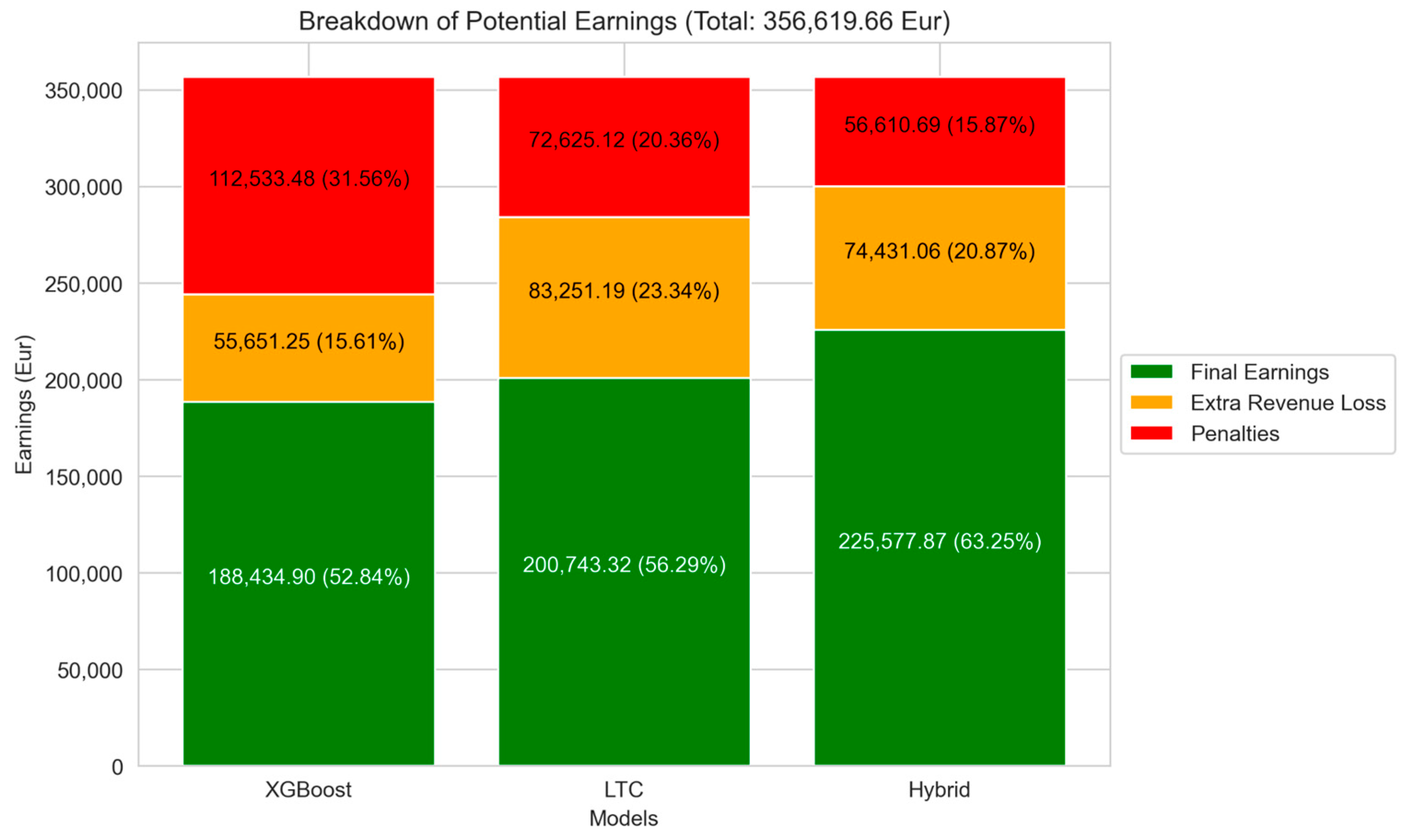
To fully assess these estimation errors, earnings should be calculated by subtracting the previously determined penalties and extra revenue losses from potential earnings (see Figure 16), which comes to a total of 356,619.66 EUR. This provides a clear understanding of the overall financial impact of each model’s estimation errors.

Total earnings are calculated as follows (see Formula (8)):

$$\sum Earnings=\sum PotentialEarnings-\sum Penalties-\sum ExtraRevenueLoss,$$

(8)

Table 14. Total earnings comparison.

Model	Earnings (Eur in Thousands)
XGBoost	188
LTC	201
Hybrid	226

demonstrates calculations of total earnings for each model. The Hybrid model has the highest earnings among all models. The hybrid model’s earnings are 16.47% higher than those of the XGBoost model and 11.01% higher than those of the LTC model, leading to maximized revenue.

Figure 16 provides a detailed breakdown of the potential composition of profits, showing once again how the accuracy of each model’s prediction can affect the financial results. From the information presented, reducing the nMAE error by 1% resulted in a profit increase of €14,739.27, representing 4.13% of total earnings.

6. Conclusions

6.1. Summary of Findings

In the course of this research, a one-year dataset was utilized for models’ training and evaluation. Based on long-term meteorological (including wind speed measurements) observations in Lithuania, this duration was deemed sufficient to develop predictive models and assess their accuracy. The data also enabled an analysis of the seasonal effects on the relationship between wind speed and wind power generation. Historical meteorological records indicate that the highest wind speeds and most frequent gusts occur during January, November, and December.

Incorporation of lags in wind power generation data enabled the development of models with higher forecasting accuracy. This strategy, while effective, presents certain challenges, as it reduces reliance on factual historical data and introduces a recursive forecasting structure. In such cases, prediction errors can propagate through subsequent time steps, potentially degrading model performance and adversely affecting long-term forecast reliability. Nevertheless, for 24-h forecasting, the careful selection of lag sets mitigated error accumulation. As a result, the models remained stable and accurate, even when part of the forecast became dependent on previously predicted values.

Based on comparative analysis, the proposed Hybrid (XGBoost + LTC) model demonstrated the highest overall forecasting accuracy (nMAE of 0.0856 and nRMSE of 0.1092) and achieved the lowest nMAE and nRMSE values with different wind speed patterns. This indicates its superior adaptability to varying weather conditions and stability compared to XGBoost and LTC models. While XGBoost performed well during calmer periods, it showed a significant increase in error during high wind fluctuation intervals. Conversely, the LTC model maintained more consistent performance across both periods, suggesting better robustness to outliers. However, the Hybrid model effectively balanced both adaptability and precision, making it the most efficient model for wind power forecasting across diverse meteorological scenarios. Furthermore, the Hybrid model showed stable performance in a 72-h forecasting period, supporting its potential for reliable medium- to long-term wind power predictions.

A comparative evaluation of forecasting models, based on findings from the literature and focused on a 24-h prediction horizon with a 1-h step, highlights the strengths and trade-offs among statistical, machine learning, and hybrid approaches. While statistical models such as SARIMA, SARIMAX, and the Markov chain achieved the lowest average nMAE (0.05265), they exhibited more dispersed errors with an average nRMSE of 0.12567. Machine learning models like LSTM, SVR, ELM, and 1D-CNN demonstrated improved short-term accuracy (average nMAE of 0.05805 and nRMSE of 0.09791), though they struggled with rapid fluctuations. In contrast, the proposed Hybrid (XGBoost + LTC) model, with an nMAE of 0.0856 and nRMSE of 0.1092, outperformed the broader group of hybrid models (average metrics of about 0.11284 for nMAE and 0.12961 for nRMSE) and offered a balanced compromise—delivering improved trend detection and more consistent error behavior across varying conditions. These findings underscore the Hybrid model’s practical value in real-world wind power forecasting scenarios.

The economic evaluation, based on hourly NordPool electricity market data and wind power forecasting results, highlights the revenue potential and stability associated with different forecasting models. Forecasts generated by the proposed Hybrid (XGBoost + LTC) model resulted in an estimated revenue increase of 16.47% compared to the XGBoost model and 11.01% compared to the LTC model. This demonstrates the Hybrid model’s superior ability to align energy production forecasts with market opportunities. Furthermore, the analysis indicates that reducing prediction error by just 1% could lead to a revenue increase of up to 4%, emphasizing the significant financial impact of improving forecast accuracy in wind energy operations.

Thus, the proposed new Hybrid (XGBoost + LTC) solution offers superior forecasting accuracy and adaptability to varying wind conditions, while maintaining stability over extended prediction horizons. Additionally, it provides significant economic benefits by aligning energy forecasts more effectively with market opportunities.

6.2. Future Research Directions

While the proposed Hybrid (XGBoost + LTC) model has demonstrated improved forecasting accuracy and economic benefits, several opportunities remain open for future research to further enhance wind power prediction and its practical applications.

First, expanding the dataset to include multi-year as well as multi-location wind data could improve model generalizability and robustness across diverse geographical and climatic conditions. This would also allow for a more accurate analysis of seasonal influences on wind power generation.

Second, future studies should investigate methods to reduce errors in the predicted meteorological elements, as these significantly impact the training and performance of forecasting models. The use of localized meteorological observation data from wind farm areas could refine input data quality and improve model accuracy.

Finally, hybridization strategies could be further refined by combining deep learning architectures (e.g., Transformers or Graph Neural Networks) with statistical models to capture both temporal dependencies and structural patterns in wind behavior. Additionally, ensemble learning approaches that dynamically weight model contributions based on recent performance could offer further accuracy gains.