Abstract
Holy basil (Ocimum tenuiflorum L.) is a medicinal herb rich in bioactive flavonoids with therapeutic properties. Traditional quantification methods rely on time-consuming and destructive extraction processes, whereas hyperspectral imaging provides a rapid, non-destructive alternative by analysing spectral signatures. However, effectively linking hyperspectral data to flavonoid levels remains a challenge for developing early detection tools before harvest. This study integrates deep learning with hyperspectral imaging to quantify flavonoid contents in 113 samples from 26 Thai holy basil cultivars collected across diverse regions of Thailand. Two deep learning architectures, ResNet1D and CNN1D, were evaluated in combination with feature extraction techniques, including wavelet transformation and Gabor-like filtering. ResNet1D with wavelet transformation achieved optimal performance, yielding an area under the receiver operating characteristic curve (AUC) of 0.8246 and an accuracy of 0.7702 for flavonoid content classification. Cross-validation demonstrated the model’s robust predictive capability in identifying antioxidant-rich samples. Samples with the highest predicted flavonoid content were identified, and cultivars exhibiting elevated levels of both flavonoids and phenolics were highlighted across various regions of Thailand. These findings demonstrate the predictive capability of hyperspectral data combined with deep learning for phytochemical assessment. This approach offers a valuable tool for non-destructive quality evaluation and supports cultivar selection for higher phytochemical content in breeding programs and agricultural applications.
1. Introduction
Holy basil (Ocimum tenuiflorum L. or Ocimum sanctum L.) is a medicinal herb in Ayurvedic medicine and has gained increasing attention in the global herbal market due to its diverse therapeutic properties [1,2]. O. tenuiflorum has been associated with various health-promoting effects. These include stress reduction, cognitive enhancement, and support for cardiovascular health [1,3,4]. This aromatic plant has been extensively studied for its rich and diverse phytochemical profile, which includes a variety of bioactive compounds such as saponins, flavonoids, terpenoids, and phenolic acids [5,6]. Saelao et al. [7] explores the antioxidant capacities of different Thai holy basil (O. tenuiflorum L.) cultivars, focusing on key compounds such as anthocyanin content, DPPH free radical scavenging activity, phenolics, flavonoids, and terpenoids content. Strong correlations among DPPH antioxidant activity, flavonoid and phenolic contents were observed. Clustering analysis revealed four distinct groups based on antioxidant profiles. The findings offer valuable insights into the potential of Thai holy basil, with variations across cultivars potentially driven by geographical factors. Among these phytochemical contents, flavonoids have emerged as a particularly significant group of secondary metabolites, renowned for their potent antioxidant, antiviral, anti-inflammatory, and potential anticancer properties [8,9,10,11]. The flavonoid composition of O. tenuiflorum is complex and varied, including compounds such as orientin, vicenin, luteolin, apigenin, and their glycosides [12,13,14]. These compounds contribute to the plant’s overall therapeutic potential [15,16].
Flavonoids are a major class of polyphenolic compounds found in O. tenuiflorum, contributing to its antioxidant and therapeutic properties. Ramsaha et al. reported that flavonoids were the predominant class of polyphenols in O. tenuiflorum species, with higher concentrations observed in the leaves of O. tenuiflorum compared to other plants [17]. This finding emphasises the potential of O. tenuiflorum as a source of natural antioxidants, which can be beneficial in food preservation and health applications. According to Tabassum et al., O. sanctum contains over 60 chemical compounds, including flavonoids, which exhibit a range of pharmacological effects such as antioxidant, anti-inflammatory, and antimicrobial activities [18]. The presence of flavonoids like vicenin-2 has been specifically noted for its potential in cancer therapy, as it has shown to inhibit Wnt/β-catenin signalling and induce apoptosis in cancer cell lines [19]. This underscores the importance of flavonoids in the plant’s therapeutic profile. The therapeutic potential of flavonoids extends to their role in managing diabetes. Research by Mousavi et al. indicated that flavonoids in O. tenuiflorum can enhance insulin sensitivity and improve glucose tolerance in diabetic models [20]. Such properties make O. sanctum a valuable candidate for developing natural remedies for diabetes management. The flavonoids present in O. sanctum Linn. play a vital role in its pharmacological activities, including antioxidant, anti-inflammatory, antimicrobial, and anti-cancer effects. The ongoing research into the extraction, identification, and application of these compounds continues to unveil the therapeutic potential of this revered herb. As the body of literature grows, it is evident that O. tenuiflorum holds promise, not only as a culinary herb, but also as a significant contributor to modern herbal medicine.
Traditional methods for quantifying flavonoids, such as high-performance liquid chromatography (HPLC) [21,22] or spectrophotometric assays [23,24], are often time-consuming, destructive, and require extensive sample preparation. In recent years, hyperspectral imaging has emerged as a promising non-destructive technique for rapid and accurate assessment of biochemical constituents [25]. This technology combines the power of spectroscopy with imaging capabilities, allowing for the collection and processing of information from across the electromagnetic spectrum [26,27]. Hyperspectral imaging generates large datasets with high spectral and spatial resolution, providing detailed information about the chemical composition of plant tissues while preserving spatial context [28]. Hyperspectral imaging combines spectroscopy and imaging to collect and process information from across the electromagnetic spectrum. This technology generates large datasets with high spectral and spatial resolution, providing detailed information about the chemical composition of plant tissues. However, the high dimensionality and complexity of hyperspectral data pose significant challenges for traditional data analysis methods.
Machine learning methods have been famous for various applications [29,30] including in plant sciences [31,32]. Recently, Suratanee et al. [33] quantified phenolic contents using hyperspectral imaging of Thai holy basil and machine learning to non-destructively assess phenolic content levels. They employed 22 statistical features extracted from hyperspectral data as inputs for classification using a neural network. The model achieved strong predictive accuracy, with a high value of area under the ROC curve for phenolic level classification. This approach offers a rapid alternative to traditional methods for antioxidant analysis and demonstrates the potential of integrating hyperspectral imaging and machine learning in plant phenotyping for phytochemical assessments. In addition to traditional machine learning algorithms, deep learning techniques, particularly Convolutional Neural Networks (CNNs), have shown remarkable success in analysing complex spectral data [34,35]. Among these, one-dimensional CNNs, such as one-dimensional residual neural networks (ResNets), have demonstrated particular efficacy in processing spectral signatures [36,37]. ResNet1D, an adaptation of the ResNet architecture for one-dimensional data, offers advantages in handling the sequential nature of spectral information while mitigating the vanishing gradient problem through residual connections.
This study aims to develop and validate a novel analysis framework for quantifying flavonoid content in basil using hyperspectral imaging coupled with ResNet1D analysis. By utilizing the power of deep learning and non-destructive imaging techniques, we seek to establish a rapid, accurate, and scalable method for assessing the nutritional and potential therapeutic value of basil. This approach has the potential to revolutionize quality control processes in the herb industry and facilitate more efficient screening of basil varieties for enhanced flavonoid content.
In the subsequent sections, we detail our comprehensive methodology encompassing holy basil cultivation, flavonoid content extraction, hyperspectral data acquisition, preprocessing protocols, feature transformation, and machine learning framework development, followed by an evaluation of deep learning models’ performance in predicting flavonoid content from hyperspectral data. The experimental design and validation strategies are thoroughly described to ensure reproducibility. We further analyse the implications of our findings for characterizing and differentiating Thai holy basil cultivars. Additionally, we discuss the key findings and implications of our integrated deep learning and hyperspectral imaging approach, providing insights for future improvements in non-destructive phytochemical analysis of medicinal herbs.
2. Materials and Methods
2.1. Plant Materials and Growing Conditions
Twenty-six accessions of local Thai holy basil (O. tenuiforum L.) were utilised in this study, comprising both standard commercially available green (G) seeds from BENJAMITR ENTERPRISE (1991) Co., Ltd., Nonthaburi, Thailand and red (R) seeds from Chia Tai Co. Ltd., Bangkok, Thailand. These local Thai accessions were generously provided by the Tropical Vegetable Research Center (TVRC) at Kasetsart University, Kamphaeng Saen Campus, Nakhon Pathom, Thailand. Seed germination followed the method described by Thongtip et al. [38] with minor modifications. Seeds were sown on germination sponges (ESPEC Corp., Osaka, Japan) under green LED lighting, providing a photosynthetic photon flux density (PPFD) of 100 μmol m−2 s−1, with a photoperiod of 16 h per day. After 14 d, seedlings with fully developed leaves were moved to a hydroponic system within a controlled environment at a plant factory utilizing artificial lighting (PFAL) for 16 d, as outlined by Chutimanukul et al. [39], before being transplanted into a greenhouse.
One-month-old plants, with seedlings having 2–3 true leaves and a shoot height of 6–10 cm, were transplanted into plastic pots (20 cm diameter) filled with commercial peat moss substrate (Hortimed SIA, Riga, Latvia). Initially, each pot received 3 g of a 16-16-16 inorganic fertilizer (N P K; nitrogen, phosphorus from P2O5, potassium from K2O). Soil moisture was maintained daily at 75–80% to support optimal plant growth. The plants were grown in a greenhouse at the Plant Phenomics Center, National Center for Genetic Engineering and Biotechnology (BIOTEC), under the National Science and Technology Development Agency (NSTDA) in Pathum Thani, Thailand. The greenhouse conditions included a 12-h photoperiod with 250 µmol m−2 s−1 of light, temperatures of 28–32 °C, relative humidity of 75–90%, and CO2 levels of 400–800 µmol mol−1 under natural sunlight.
Holy basil plants were harvested three times at full bloom, with three harvests occurring: the first harvest occurred 42 d after transplanting, the second at 63 d, and the third at 84 d. Hyperspectral images of the plants were captured using a hyperspectral camera (Photon Systems Instruments, spol.s r.o.; Drásov, Czech Republic) and analysed with PlantScreen™ data analyser software (version 3.1.7.21). After measuring the hyperspectral imaging, canopy leaves were harvested for analysis of flavonoid quantification.
2.2. Flavonoid Content Extraction
Fresh holy basil canopy leaves were dried at 40 °C for 72 h. The dried leaf tissue was then ground into a fine powder using a pestle. Extractions were carried out using a modified method [39]. Specifically, 10 mg of fine powder was extracted with 5 mL of absolute methanol (99.9%, HPLC grade, FISHER, Waltham, MA, USA) containing 1% HCl. The mixture was thoroughly vortexed and incubated at 25 °C for 3 h. After incubation, the solution was centrifuged at 15,249× g for 5 min using an Eppendorf Centrifuge 5810R equipped with a rotor F-34-6-38 (6 × 125 g). After extraction, the supernatant was transferred to a separate microcentrifuge tube (2 mL) for subsequent assessment of flavonoid content
The total flavonoid content was quantified using a colorimetric method, following the procedure outlined by Chutimanukul et al. [40] and Bao et al. [41], with slight modifications. A 350 µL aliquot of the extracted solution was combined with 75 µL of 5% sodium nitrite (NaNO2) in a 1.5 mL microcentrifuge tube, then centrifuged at 12,000 rpm for 2 min at 25 °C. After allowing the mixture to rest at room temperature for 5 min, 75 µL of 10% aluminium chloride (AlCl3·6H2O) was added and thoroughly mixed via vortex mixer. The reaction mixture was centrifuged again and left to stand for another 5 min. Subsequently, 1 M sodium hydroxide (NaOH) was added. The homogenised solution was centrifuged and maintained at 25 °C for 15 min. Absorbance was measured at 515 nm using a spectrophotometer (Multiskan Sky, Thermo Fisher Scientific, Waltham, MA, USA). The total flavonoid content was calculated based on a standard curve of rutin dissolved in dimethyl sulfoxide (DMSO), with the concentration expressed as milligrams of rutin equivalents per gram of dry weight (DW).
2.3. Determination of Flavonoid Content Level
To classify flavonoid content levels in holy basil samples, we developed a thresholding method based on both biological reference and statistical rigour. Flavonoid levels were first measured in standard green and red cultivars to establish a reference distribution. The mean flavonoid content among these reference samples was 20.2302 mg rutin/gDW, with a standard deviation of 6.2884 mg rutin/gDW. Rather than using the mean as a simple cutoff, we selected a more conservative threshold set at 1.2 standard deviations below the mean to account for natural biological variability and to more effectively distinguish lower-flavonoid samples. This resulted in a cutoff value of 12.6841 mg rutin/gDW. Samples with flavonoid content greater than or equal to this cutoff were labelled as normal-to-high, while those below the cutoff were categorized as low. This classification strategy was then used in the deep learning framework to differentiate between the two flavonoid content categories.
2.4. Hyperspectral Image Acquisition and Data Preprocessing of Holy Basil
A PlantScreenTM system was employed for hyperspectral data collection. Hyperspectral images (510 × 550 pixels) of fresh holy basil were captured across two spectral ranges: visible-near infrared (VNIR, 355–900 nm) and shortwave infrared (SWIR, 900–1700 nm), yielding 1116 spectral bands within the 355–1700 nm range. Images were segmented to isolate holy basil parts, with backgrounds removed. PlantScreenTM software (version 3.1.7.21) converted images into spectral data, mitigating multicollinearity issues and calculating average spectra and standard deviations for each sample. Data were initially categorized into three groups based on plant age: first cut at 42 d, second cut 21 d after the initial leaf cutting, and third cut 21 d after the second cut. To reduce dimensionality, spectral data were sampled at 2 nm wavelength intervals. Based on analysis from the previous study [33], which showed that data from the first cut deviated significantly from the others, we selected only data from the second and third cuts for our current analysis.
2.5. Hyperspectral Data Transformations
Prior to classification, we conducted experiments to transform the hyperspectral data into more informative feature representations. Two key feature extraction techniques were employed: wavelet transformation and Gabor-like filtering. The wavelet transformation enabled us to capture multi-scale frequency information from the input data, while Gabor-like filtering, which is widely used in signal processing, was employed to capture both spatial (or temporal) and frequency information from the signal. This approach is particularly effective for analysing localized frequency variations in spectral data. These preprocessing steps enhanced the discriminative power of the input data, potentially improving the model’s ability to differentiate between various levels of flavonoid content.
2.5.1. Wavelet-Based Feature Extraction
To extract meaningful features from the spectral data, we employed a wavelet-based feature extraction technique using the Discrete Wavelet Transform (DWT). This method is particularly effective for analysing signals across multiple scales and capturing both time-domain and frequency-domain characteristics, making it suitable for the spectral data used in this study.
The wavelet decomposition was performed using the Daubechies 4 (db4) wavelet, a commonly used wavelet family known for its ability to effectively capture both smooth and abrupt changes in the signal. The DWT performs a multilevel decomposition of the input signal, where the signal is split into approximation and detail coefficients at each level. The approximation coefficients capture the low-frequency components of the signal, while the detail coefficients capture the high-frequency components. For a given signal S(t), the DWT decomposes the signal into approximation and detail coefficients up to a specified level L. The decomposition can be represented as:
where represents the approximation coefficients at level , containing the low-frequency components. are the detail coefficients at level 1 to , capturing the high-frequency components. In this study, we decomposed each spectral signal up to level 4, meaning that the signal was decomposed into one set of approximation coefficients () and four sets of detail coefficients (). This approach allows us to retain information from different scales of the data, which is essential for analysing complex patterns in the spectra. The process began by applying the DWT to each spectrum in the dataset, resulting in a set of wavelet coefficients for each decomposition level. These coefficients represent different frequency bands of the signal, with lower levels corresponding to higher frequency details and higher levels capturing lower frequency, smoother components. The wavelet coefficients from all decomposition levels were then concatenated to form a feature vector of length 699 for each spectrum. In this study, we used the PyWavelets module in Python (version 3.11.13) for wavelet transformation. Given the varying scales of the wavelet coefficients, we applied MinMax scaling from the sklearn module to normalize the feature values, transforming them to a range between 0 and 1. This ensures that all features are treated uniformly during model training and prevents any single feature from disproportionately influencing the learning process. This wavelet-based approach provides a comprehensive representation of the spectral data, capturing both local variations and global trends. The resulting features are used as input for the classification model, enhancing its ability to differentiate between classes based on the spectral characteristics of the data.
2.5.2. Gabor-like Feature Extraction for Spectral Data
In addition to wavelet transformation, to extract meaningful features from the spectral data, we applied a Gabor filtering technique that utilizes convolution with a set of custom-designed 1D filters. Gabor-like filters are particularly effective for capturing both frequency and spatial (or temporal) information by combining a Gaussian envelope with a sinusoidal wave, making them well-suited for analysing signals with localized frequency characteristics.
In the general form, a complex 1D Gabor filter can be represented as follows:
where controls the spread of the Gaussian envelope, and denotes the frequency of the oscillatory component. The complex exponential can be expanded using Euler’s formula:
For simplicity, we utilized only the real part of the 1D Gabor filter, given by:
The real component effectively captures even-symmetric features in the spectral data, such as edges and peaks, which are often of primary interest when analysing spectral signals.
The feature extraction process involved convolving the spectral data with Gabor-like kernels at various frequencies and scales, defined by and . The 1D Gabor kernel used in the convolution is defined as:
where represents the position of the spectral data, is the frequency, and controls the width of the Gaussian envelope, and is the kernel length. The summation over is computed once for the entire kernel to normalize it prior to convolution with the spectral data. The normalized kernel is then convolved with the spectral data by sliding it across the entire signal. At each position , the kernel is multiplied element-wise with the corresponding section of the spectral data, and the products are summed to produce the filtered signal. This convolution captures local frequency information in the spectral data, highlighting features such as peaks, and periodic structures.
We selected a range of frequencies and Gaussian widths () to capture features at multiple scales and frequency resolutions. The filtered spectrum, , was computed by convolving the input spectrum with the Gabor kernel:
In this notation, represents the discrete convolution operation, which slides the Gabor kernel across the entire spectrum . From the filtered spectrum, a set of statistical features was extracted. The feature is the mean absolute value of the filtered signal, which can be described as:
where is the length of the spectrum. This feature reflects the overall intensity of the spectral signal at a given frequency and scale, summarizing the local frequency content of the data. We used 12 distinct frequencies (0.1, 0.25, 0.5, 0.75, 1.0, 1.25, 1.5, 1.75, 2.0, 2.25, 2.5, and 2.75) and 8 Gaussian widths () ranging from 1 to 8 to create a comprehensive set of features. For each combination of frequency and sigma, a unique feature was computed, resulting in a feature vector of length 96 for each spectrum. This feature extraction method was applied to all spectral samples in the dataset, and the extracted features were subsequently used as input to machine learning models for classification and analysis. The use of Gabor-like filtering provided a robust approach to capture frequency-localized information across multiple scales, enhancing the predictive performance of the model.
2.6. Data Preparation
Hyperspectral data samples of Thai holy basils were initially collected. These data underwent preprocessing using the Multiplicative Scatter Correction (MSC) algorithm to reduce the effects of light scattering and improve the quality of spectral measurements. To ensure data integrity, outlier samples were identified and removed based on an absolute z-score threshold of 3. The samples were then categorized into two groups based on their flavonoid contents, using a predetermined cutoff threshold to distinguish between low and normal-to-high levels (see Section 2.3). The processed dataset was then used for feature transformations and classification analysis.
2.7. Deep Learning Architecture and Parameters
In this study, we employed a one-dimensional residual neural network (ResNet1D) architecture, as shown in Figure 1, to perform classification tasks on transformed spectral data. The architecture employs residual connections to mitigate the vanishing gradient problem and facilitate the training of deeper models, thereby improving generalization and accuracy on complex datasets. Our model is specifically designed for processing 1D data, making it suitable for applications such as time-series analysis and sequential data classification. The ResNet1D architecture begins with an initial convolutional layer (Conv 1D) that applies a 1D convolution operation to the input data, with a kernel size of 7 and a stride of 2, followed by batch normalization (BatchNorm 1D) and a ReLU activation function. This combination of layers serves to extract low-level features from the input data. A max-pooling layer (MaxPool1D) is then applied, reducing the dimensionality of the input and increasing computational efficiency.
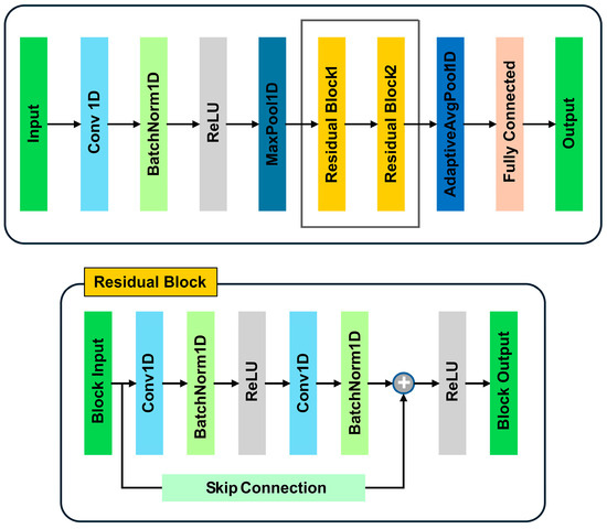
Figure 1.
Deep learning architecture.
The core of the network consists of two residual blocks, each composed of two convolutional layers interspersed with batch normalisation and ReLU activations. Each residual block is equipped with a shortcut (skip connection) that bypasses the convolutional layers, directly adding the input to the block’s output. This allows the network to preserve gradient flow during backpropagation, enabling deeper models to be trained effectively without suffering from performance degradation. The first residual block maintains the same number of channels, while the second block doubles the number of channels and reduces the spatial resolution through downsampling. This structure allows the network to capture both local and global patterns in the data. After passing through the residual blocks, the feature map is further reduced by an adaptive average pooling layer (Adaptive AvgPool 1D), which pools the feature map to a fixed length of one, irrespective of the original input length. This ensures compatibility with fully connected layers, regardless of the input sequence’s length. The resulting feature vector is passed to a fully connected layer for final classification. The output of the fully connected layer represents the class probabilities, which are computed using the softmax function for multi-class classification. To stabilise training and prevent overfitting, batch normalization is applied throughout the network. The network was trained using the Adam optimiser with a learning rate of 0.001, and cross-entropy loss was employed as the loss function. During training, the model’s parameters were updated using gradient-based optimisation to minimize the classification error over a series of epochs. This ResNet1D architecture incorporates residual connections, batch normalisation, and adaptive pooling, making it a robust and efficient solution for 1D data classification tasks. Its ability to handle long sequences and complex patterns makes it well-suited for a variety of applications, including time-series analysis and medical signal classification.
2.8. Model Training and Evaluation
We employed a rigorous model training and evaluation process using repeated stratified k-fold cross-validation to ensure robust performance assessment. The dataset was randomly split into 10 stratified repeats, each consisting of 5 folds, ensuring balanced representation of both classes in each fold. This approach helps mitigate any potential biases introduced by data imbalance and provides a reliable estimate of the model’s performance across different data partitions. We performed hyperparameter tuning using a grid search method to identify the optimal configuration of learning rate, batch size, and the number of epochs. Specifically, the hyperparameter grid included the learning rate (0.01), batch sizes (16, 32), and training epochs (50, 100). The model’s performance was evaluated using the accuracy metric as the primary criterion for optimization during grid search. To address class imbalance, we employed a downsampling technique to balance the classes within the training set. In each fold, the minority class was identified, and an equal number of samples from the majority class were randomly selected to match the size of the minority class. This process was performed to ensure that the model was trained on balanced data in each fold.
In addition, we utilized recursive feature elimination with cross-validation (RFECV) to identify the most relevant features for classification. A logistic regression model was employed as the base estimator for RFE, with a step size of 10% and a minimum of 150 features retained to ensure that the model had sufficient input dimensions to perform effectively. RFECV was performed within each fold to ensure that feature selection was applied independently to each training set, further reducing the risk of overfitting and ensuring that the selected features generalize well across different data splits. After feature selection, the training data was converted to be used with our custom ResNet1D model. A newly instantiated model was trained for each fold, using the cross-entropy loss function and the Adam optimiser with a learning rate of 0.001. For each training session, the model parameters were optimised to minimize the classification error over a series of epochs, and early stopping was employed to prevent overfitting.
The model’s predictive performance was evaluated using two key metrics: accuracy and area under the receiver operating characteristic curve (AUC). Accuracy (ACC) measured the proportion of correctly classified samples, while AUC assessed the model’s ability to discriminate between normal-to-high and low flavonoid content levels. The AUC was computed for the normal-to-high class (positive class) using the predicted probabilities from the model’s output. The accuracy was calculated using an optimal threshold determined by Youden’s J statistic to classify samples into normal-to-high or low groups based on their predicted probabilities. The repeated stratified k-fold cross-validation approach provided a robust estimate of the model’s performance, mitigating potential biases from random data partitioning or class imbalance. The final performance metrics were calculated by averaging the accuracy and AUC scores across all repetitions.
3. Results
3.1. Overview
Our study focused on the analysis of hyperspectral imaging data of Thai holy basil (O. tenuiflorum L.) and its antioxidant properties, specifically the flavonoid content. Hyperspectral imaging provides a wealth of spectral information, allowing for detailed analysis of plant biochemical composition. We obtained reflectance data from the samples, which served as our spectral dataset. To enhance the quality and interpretability of this data, we applied several preprocessing techniques. The primary goal of our research was to investigate the relationship between the processed spectral data and the flavonoid content of the Thai holy basil samples. To achieve this, we employed advanced deep learning models, which have shown great promise in extracting meaningful patterns from complex spectral data. This approach allows us to potentially develop a non-destructive method for estimating flavonoid content in Thai holy basil, which could have significant implications for quality control and optimization in herbal medicine and the food industry. The overview of our analysis is shown in Figure 2.
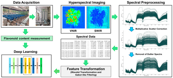
Figure 2.
Overview of the analysis framework.
The framework, illustrated in Figure 2, begins with data acquisition during the growth of the plants, where we collect flavonoid content and capture hyperspectral imaging (both for VNIR and SWIR; more details are provided in Section 2). The level of flavonoid content for each sample is categorized into two classes: low and normal-to-high levels. The spectral data is then processed and transformed to better capture its features. Finally, deep learning techniques, including ResNet1D and CNN1D, are applied to classify and identify the flavonoid levels for each sample.
We collected a total of 237 hyperspectral data samples of Thai holy basil. After preprocessing with the Multiplicative Scatter Correction (MSC) algorithm and removing outliers (see Section 2), we refined the dataset to 229 samples. Based on a predetermined cutoff threshold, we categorized the samples into two groups: 58 samples in the low group and 171 in the normal-to-high group. These processed data were subsequently used for classification analysis.
3.2. Efficacy of Flavonoid Content Level Classification Using ResNet1D and Feature Transformation Techniques
Our study focused on classifying flavonoid content levels in hyperspectral data using advanced machine learning techniques. We employed a ResNet1D architecture as our primary classification model. To enhance the model’s ability to extract meaningful features from the complex hyperspectral data, we performed an experiment incorporating two well-known feature transformation techniques: wavelet transformation and Gabor-like filtering. These transformations were integrated into our preprocessing pipeline to generate discriminative features that enhanced the model’s classification performance. Our experimental design involved a rigorous ten-time five-fold cross-validation approach. This method ensures robust evaluation by dividing the dataset into five parts, using four for training and one for testing, and repeating this process ten times with different random splits. This approach helps to mitigate bias and provides a more reliable estimate of the model’s performance. During the training phase in each fold, we balanced the two classes by randomly downsampling the majority class to match the number of samples in the minority class. This balancing step was employed to prevent bias in the model’s learning process. By ensuring equal representation of both classes in the training data, we aimed to develop a model that could accurately classify both ‘normal-to-high’ and ‘low’ flavonoid content levels without favouring one class over the other.
Using wavelet transformation and Gabor-like filtering to generate features, we obtained promising results, with an AUC of 0.8136 ± 0.0159 (mean ± standard deviation) and an ACC of 0.7461 ± 0.0326 (mean ± standard deviation). The high AUC score of 0.8136 indicates strong discriminative power to distinguish between ‘normal-to-high’ and ‘low’ flavonoid content levels. This suggests that our model can effectively separate the two classes, which is crucial for accurate classification in practical applications. The relatively low standard deviation of the AUC (0.0159) suggests consistent performance across different repetition experiments. This consistency is important as it indicates that our model’s performance is robust and not overly sensitive to the specific data split used in each fold of the cross-validation. The accuracy measure (ACC) provides additional insight into the model’s overall classification performance. While the ACC is also high at 0.7461, it shows more variability (standard deviation of 0.0326) compared to the AUC metric. This higher variability in ACC could be due to factors such as class imbalance or the specific threshold chosen for classification.
These results demonstrate the effectiveness of our approach in classifying flavonoid content levels. The combination of the ResNet1D architecture with wavelet transformation and Gabor-like filtering for feature extraction appears to be a powerful method for handling the complexities of hyperspectral data in this context. The high AUC and ACC scores suggest that this approach could be valuable in practical applications where accurate classification of flavonoid content is crucial.
To evaluate the independent contributions of each feature extraction methods, we conducted systematic ablation studies comparing the performance of different feature combinations. In the first experiment, we removed Gabor-like filtering features while retaining wavelet transformation. Interestingly, this modification improved model performance, yielding an AUC of 0.8246 ± 0.0180 and ACC of 0.7702 ± 0.0188. Conversely, when we isolated Gabor-like filtering features by removing wavelet transformation, the model’s performance decreased substantially, achieving an AUC of 0.6869 ± 0.0531 and ACC of 0.6948 ± 0.0440. These results reveal distinct contributions from each feature extraction method. Removing Gabor-like filtering features led to an improvement in AUC (from 0.8136 to 0.8246) and a high improvement in ACC (from 0.7461 to 0.7702). This suggests that Gabor-like filtering features may introduce noise that slightly impairs the model’s discriminative capabilities. In contrast, discarding wavelet transformation features resulted in a more substantial decrease in both AUC (from 0.8136 to 0.6869) and ACC (from 0.7461 to 0.6948), indicating that wavelet transformation plays a crucial role in generating discriminative features for flavonoid content classification. These findings demonstrate that wavelet transformation alone provides optimal performance in our classification task. While the combination of both methods yields competent results, it performs slightly more poorly than wavelet transformation alone. Using Gabor-like filtering in isolation leads to notably lower performance. These results demonstrate that wavelet transformation is the most effective feature extraction technique for flavonoid content level classification. The performances are summarised in Table 1.

Table 1.
Performance comparison of ResNet1D using different feature combinations (wavelet transformation and Gabor-like filtering).
To further investigate the importance of both wavelet transformation and Gabor-like filtering, we evaluated the ResNet1D architecture using hyperspectral data without any feature transformation methods. Using this data, the model demonstrated significantly lower performance, with an AUC of 0.6484 ± 0.0353 and ACC of 0.6369 ± 0.0388. This marked decrease in performance compared to our original results (AUC: 0.8136 ± 0.0159, ACC: 0.7461 ± 0.0326) demonstrates the crucial role of feature extraction in enhancing the model’s classification capabilities. Without these transformations, the model’s ability to discern meaningful patterns in the complex hyperspectral data is substantially reduced. These findings validate the effectiveness of our feature extraction approach in preprocessing hyperspectral data for flavonoid content classification using deep learning architectures.
3.3. Analysis of CNN1D Architectures for Flavonoid Content Classification
To further evaluate our approach and assess the influence of network architecture on classification performance, we conducted additional experiments using an alternative deep learning structure. While our primary results were obtained with the ResNet1D architecture, we sought to understand the impact of its key architectural feature—namely, the shortcut connections or skip connections. To this end, we developed a simpler one-dimensional convolutional neural network (CNN1D) that shares structural similarities with ResNet1D, such as the use of convolutional layers and batch normalization, but crucially omits the skip connections. Using this CNN1D structure with both wavelet and Gabor-like filtering features, we achieved strong performance, with an AUC of 0.7911 ± 0.0389 and ACC of 0.7336 ± 0.0455. Following the trend observed in our ResNet1D experiments, using wavelet transformation alone yielded superior results, with an AUC of 0.8190 ± 0.0248 and ACC of 0.7618 ± 0.0169. Conversely, when using Gabor-like filtering alone, performance decreased notably, resulting in an AUC of 0.6809 ± 0.0496 and ACC of 0.6817 ± 0.0560. Similar to our ResNet1D experiments, using hyperspectral data without feature extraction led to significantly lower performance, with an AUC of 0.6555 ± 0.0187 and ACC of 0.6510 ± 0.0518.
These results demonstrate that the relative effectiveness of different feature extraction methods remains consistent across architectures, with wavelet transformation consistently outperforming Gabor-like filtering. However, the overall performance metrics suggest that the ResNet1D architecture’s skip connections provide a modest advantage in classification accuracy compared to the simpler CNN1D structure. This indicates that while both architectures are capable of effectively leveraging the extracted features, the additional complexity of ResNet1D’s skip connections contributes to enhanced model performance. The complete performance metrics are summarised in Table 2.
Table 2.
Performance comparison of CNN1D using different feature combinations (wavelet transformation and Gabor-like filtering).
3.4. Effects of Feature Selection on Classification Performance
Feature selection techniques can often enhance classification performance by identifying the most relevant features for the task. In this study, we employed RFECV, an iterative feature selection method that recursively removes features and builds models on the remaining features, using model accuracy to identify the most predictive feature combinations. We implemented RFECV with a minimum threshold of 150 features to balance dimensionality reduction with maintaining sufficient complex features for effective deep learning pattern extraction.
We evaluated the impact of RFECV by comparing model performance with and without feature selection. When applying RFECV to the combined wavelet transformation and Gabor-like filtering features, both architectures showed improved performance: ResNet1D achieved an AUC of 0.8223 ± 0.0722 and ACC of 0.7541 ± 0.0264, while CNN1D yielded an AUC of 0.8230 ± 0.0177 and ACC of 0.7629 ± 0.0215. However, when applying RFECV to wavelet features alone, both models showed slightly decreased performance. ResNet1D achieved an AUC of 0.8152 ± 0.0272 and ACC of 0.7410 ± 0.0315, while CNN1D achieved an AUC of 0.8134 ± 0.0256 and ACC of 0.7523 ± 0.0339.
For configurations using only Gabor-like filtering, RFECV had no impact as the number of features (96 features) was below our preset minimum threshold of 150 features, resulting in identical performance with and without RFECV. When applying RFECV to hyperspectral data without feature extraction methods, we observed improved performance in both architectures: ResNet1D showed substantial improvement with an AUC of 0.6980 ± 0.0351 and ACC of 0.6899 ± 0.0429, while CNN1D showed modest gains with an AUC of 0.6643 ± 0.0656 and ACC of 0.6690 ± 0.0540.
These results suggest that RFECV’s effectiveness varies depending on the feature extraction method employed. While RFECV improved performance when applied to combined features (wavelet and Gabor-like filtering features) or hyperspectral data without feature extraction, it slightly decreased performance when applied to wavelet features alone. This indicates that wavelet transformation may already provide an optimal feature set for classification, and further feature selection could potentially remove informative features. The similar performance patterns observed across both ResNet1D and CNN1D architectures further validate these findings. Notably, across all experimental configurations, the highest classification performance was achieved using ResNet1D with wavelet features alone, without applying RFECV. The complete performance metrics are summarised in Table 3. The overall performance metrics of all experiments are visualised by ROC curves and shown in Figure 3.
Table 3.
Performance comparison of ResNet1D and CNN1D using different feature extraction configurations With RFE.
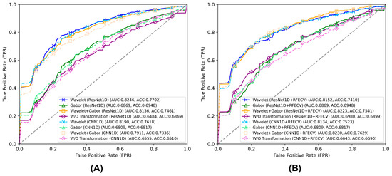
Figure 3.
ROC curves and performance comparison of (A) ResNet1D and CNN1D models using different types of feature transformations and (B) the same algorithms integrated with recursive feature Elimination with cross-validation (RFECV). The performances of Gabor-like filtering with RFECV are identical to those without RFECV. This is because RFECV had no impact on the configuration with Gabor-like filtering, as the number of Gabor-like filtering features (96) was below the preset minimum threshold of 150 features.
3.5. Identification of Samples with High Flavonoid Content Levels from Deep Learning Predictions
The ResNet1D architecture with wavelet features was utilized for predictions, with each sample evaluated through a ten-fold cross-validation process repeated five times. Predictions from individual models were aggregated, and the median value was calculated as the final score for each sample. Scores approaching 1.0 indicated high confidence in predicting elevated flavonoid content. The ROC curve calculated from final scores and labels is presented in Figure 4A, yielding an AUC of 0.8696 and accuracy of 0.8210 (determined using Youden’s J statistic). Using this statistic, we identified an optimal threshold of 0.3188 that balances sensitivity and specificity. The red dot on the ROC curve in Figure 4A represents the optimal operating point (false positive rate: 0.1724, true positive rate: 0.8187). Samples with scores greater than or equal to this threshold were classified as normal-to-high flavonoid content level, while those below the threshold were classified as low flavonoid content level. The distribution of flavonoid contents between these two groups showed significant difference (p-value = 1.0439 × 10⁻¹⁴) as shown in the boxplot in Figure 4B. A complete list of samples with their prediction scores is presented in Table S1.
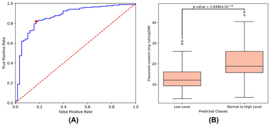
Figure 4.
(A) ROC curve derived from the prediction scores of the ResNet1D model with wavelet transformation. The blue line represents the ROC curve, the red dashed line indicates the performance of random classification, and the red dot marks the optimal operating point that balances sensitivity and specificity. (B) Box plot illustrating the separation of flavonoid content between low and normal-to-high groups based on the predicted classes.
To identify samples with high confidence predictions, we selected those with scores greater than or equal to 0.95. This selection yielded 113 samples with confirmed normal-to-high flavonoid levels. These samples represented 18 different cultivars collected from various locations in Thailand, including both commercial varieties (Green and Red) and local accessions. Analysis of the harvest cuts revealed a distinct pattern in our dataset. Among the selected samples, there was a clear predominance of Cut 3 samples (78 samples, 69.0%) compared to Cut 2 samples (35 samples, 31.0%). Cut 3 samples generally showed higher flavonoid content, ranging from 9.10 to 45.02 mg rutin/gDW, with particularly high levels observed in samples from Damnoen Saduak, Ratchaburi (45.02 mg rutin/gDW) and Kamphaeng Saen, Nakhon Pathom (43.52 mg rutin/gDW). In contrast, Cut 2 samples exhibited a different range of flavonoid content, typically between 4.97 and 29.52 mg rutin/gDW, with the highest content found in samples from Mueang Lampang, Lampang (29.52 mg rutin/gDW). To statistically assess the observed differences, we performed a Mann–Whitney U test comparing flavonoid content between Cut 2 and Cut 3 samples (score ≥ 0.95). The test confirmed a significant difference between the two groups (p-value = 2.1202 × 10⁻¹⁰), supporting the pattern that Cut 3 samples tend to have higher flavonoid levels. The prediction scores also showed interesting cut-related patterns. While both cuts achieved high prediction scores (≥0.95), Cut 3 samples dominated the highest-scoring range (>0.999), suggesting that the model identified more distinctive spectral features associated with flavonoid content in these samples. This pattern might be attributed to the plants’ physiological maturity in the third harvest cycle or potentially more favourable environmental conditions during this growth period.
Table 4 shows the top 25 samples with the highest prediction scores (0.999962 to 0.999999). Within this subset, 23 samples were from Cut 3 and only two samples from Cut 2, further emphasizing the dominance of Cut 3 samples among the highest-confidence predictions. The flavonoid content values for each sample are representative of the entire sample set, which includes a wider range of cultivars to display a broader spectrum of flavonoid content. These top samples displayed flavonoid content on average 23.35 mg rutin/gDW, with notably high levels observed in samples from Damnoen Saduak, Ratchaburi (45.02 mg rutin/gDW) and Wat Phleng, Ratchaburi (40.43 mg rutin/gDW). Commercial varieties from Chia Tai Co. Ltd., BENJAMITR ENTERPRISE (1991) Co., Ltd., and local accessions from various regions consistently appeared in this top-scoring group, suggesting that both cultivated and local varieties can achieve high flavonoid content under appropriate growing conditions.
Table 4.
Top 25 samples with high prediction scores for flavonoid contents.
3.6. Identification Samples with High Phenolics and Flavonoid Contents
From our previous study, we identified samples that showed high phenolic contents. Of particular interest were samples that exhibited both high phenolic and high flavonoid contents. We focused on samples meeting two criteria: prediction scores ≥ 0.95 and normal-to-high range values for both flavonoid contents (current study) and phenolic contents (previous study). This analysis yielded 108 samples for flavonoid content prediction and 20 samples for phenolic content prediction, with 18 samples overlapping between these groups, as shown in Table 5. These 18 overlapping samples showed phenolic content prediction scores ranging from 0.950039 to 0.995552, while flavonoid content prediction scores were consistently higher, ranging from 0.999949 to 0.982816. The samples were predominantly from Cut 3 (16 samples), with only two samples from Cut 2, and were collected from various locations across Thailand, including Lopburi, Udon Thani, Roi Et, Ratchaburi, Bangkok, Phitsanulok, Chiang Rai, Rayong, Phrae, and Songkhla. The phenolic contents varied from 26.1395 to 36.5657 mg GAE/gDW, with the highest content observed in the commercial variety from Chia Tai Co. Ltd. (3-PS_Tray_200-Green), followed by samples from Mae Lao, Chiang Rai (34.3301 mg GAE/gDW) and Chai Badan Lop Buri (33.1466 mg GAE/gDW). The flavonoid contents ranged from 16.7679 to 38.9544 mg rutin/gDW, with the highest content found in the sample from Chai Badan, Lopburi (OC063), followed by samples from Mueang Rayong, Rayong (37.4741 mg rutin/gDW) and Udon Thani (36.9242 mg rutin/gDW). Notably, some locations, such as Mae Lao, Chiang Rai (OC148), Chai Badan, Lopburi (OC063) and Udon Thani (OC194), were represented by multiple samples, suggesting consistent phytochemical profiles within certain geographical regions. We used a map of Thailand to depict the provinces where cultivars were predicted to have high contents of both flavonoids and phenolics, as well as those with high flavonoid content only. This illustration is presented in Figure 5.
Table 5.
Comparison of samples with high prediction scores (≥0.95) for both phenolic and flavonoid contents, showing their median scores, measured contents, and collection locations across Thailand.
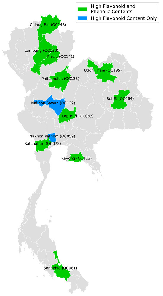
Figure 5.
Locations of cultivars (provinces in Thailand) predicted to have high flavonoid and phenolic contents.
4. Discussion
The results highlight the effectiveness of both ResNet1D and CNN1D architectures for our classification problem, with ResNet1D showing slightly better performance in most configurations. The modest performance advantage of ResNet1D suggests that its skip connections contribute positively to feature extraction and classification accuracy in hyperspectral data analysis.
The effectiveness of different feature extraction methods varied significantly in our experiments. Wavelet transformation consistently demonstrated superior performance across both architectures, particularly when used independently. Notably, ResNet1D with wavelet transformation alone achieved the best overall performance (AUC: 0.8246 ± 0.0180, ACC: 0.7702 ± 0.0188), surpassing even the combined feature approach. When used independently, Gabor-like filtering showed notably lower performance compared to wavelet transformation in both architectures. Combining Gabor-like filtering with wavelet transformation led to slightly decreased performance compared to using wavelet transformation alone. This suggests that Gabor-like filtering features might introduce noise that slightly impairs the model’s discriminative capabilities when combined with wavelet features. Additionally, the superior performance of the wavelet transformation over Gabor-like filtering may be due to its ability to capture both global and local spectral features through multiresolution analysis using the Discrete Wavelet Transform (DWT) with Daubechies 4 (db4). Unlike Gabor filters, which reduce each filtered signal to a single value and risk losing important details, the wavelet method preserves a richer set of features across multiple frequency levels. This flexibility allows wavelets to better capture non-stationary and multiscale patterns typical in hyperspectral plant data.
The importance of feature extraction methods was further demonstrated in experiments without any feature extraction, where both architectures showed substantially lower performance. ResNet1D without feature extraction achieved an AUC of 0.6484 ± 0.0353 and ACC of 0.6369 ± 0.0388, while CNN1D showed similar results, with an AUC of 0.6555 ± 0.0187 and ACC of 0.6510 ± 0.0518. The application of RFECV showed varying effects depending on the feature extraction method used. While RFECV improved performance when applied to combined features or hyperspectral data without feature extraction, it slightly decreased performance when applied to wavelet features alone. This suggests that wavelet transformation may already provide an optimal feature set, and additional feature selection could potentially remove informative features.
These findings indicate that, while both architectures are effective for our classification task, the choice of feature extraction method plays a more crucial role in determining overall performance than the choice of network architecture. Wavelet transformation emerges as the most effective single method for feature extraction in our classification framework. Notably, our experiments revealed that classifying flavonoid content levels using hyperspectral data presents greater challenges compared to phenolic content classification in previous studies [33]. Using the same traditional statistical features (22 features) with neural networks that were effective for phenolic content classification, we achieved an AUC of 0.7603 ± 0.0187 and accuracy of 0.7201 ± 0.0281 for flavonoid content classification. These results are lower than the performance achieved using our proposed feature extraction methods with ResNet1D and CNN1D architectures. This improvement in performance demonstrates the superiority of our proposed approach combining deep learning architectures with advanced feature extraction methods over traditional statistical feature-based approaches for complex flavonoid content classification tasks.
Both phenolic and flavonoid contents are important phytochemicals in holy basil. We identified samples that showed high contents of both compounds. Interestingly, the majority of these samples were from Cut 3, indicating that the maturity stage might influence both phenolic and flavonoid accumulation in Thai holy basil. The broad geographical distribution of O. tenuiflorum L. samples across Thailand, from the northern region (Chiang Rai) to the southern region (Songkhla), demonstrates the adaptability of this medicinal herb to different environmental conditions while maintaining high phytochemical contents. Notably, the commercial variety from Chia Tai Co. Ltd. exhibited the highest phenolic content (36.5657 mg GAE/gDW), suggesting successful breeding selection for this trait. Meanwhile, the local variety from Chai Badan, Lopburi showed the highest flavonoid content (38.9544 mg rutin/gDW), highlighting the potential value of local O. tenuiflorum varieties for future breeding programs. The consistently high prediction scores for both compounds, particularly for flavonoids (up to 0.99999), indicate the robust reliability of our prediction models in identifying holy basil varieties rich in these beneficial compounds. These findings provide valuable information for selecting promising holy basil varieties for breeding programs aimed at enhancing nutritional quality and antioxidant properties.
Despite the promising performance of the deep learning models in quantifying flavonoid contents from hyperspectral data, some limitations should be acknowledged. While the sample size was adequate for initial model development, it remains relatively limited, which may affect the generalisability of the models to broader holy basil populations. Additionally, the hyperspectral imaging was performed under controlled laboratory conditions. Environmental variations—such as natural light, temperature, and leaf orientation in field settings—were not considered in this study, which might impact the robustness and applicability of the models in real-world agricultural scenarios. Furthermore, while the model effectively classified flavonoid content based on spectral information, we did not perform a direct analysis of the correlation between specific spectral bands and flavonoid concentration. Identifying key wavelength regions associated with flavonoid absorption could enhance biological interpretability and inform the development of targeted sensing strategies. These limitations highlight opportunities for future studies to improve model robustness and generalizability under practical field conditions.
5. Conclusions
This study demonstrates the effectiveness of deep learning approaches combined with feature extraction methods for classifying flavonoid content levels in holy basil using hyperspectral imaging data. Our findings reveal that ResNet1D architecture generally outperforms CNN1D, highlighting the advantages of skip connections for complex spectral data analysis. The evaluation of different feature extraction methods showed that wavelet transformation consistently provided superior performance across architectures, while Gabor-like filtering exhibited lower performance when used independently. Notably, the combination of both methods did not improve performance compared to wavelet transformation alone, suggesting that wavelet features may be optimal for this classification task.
The investigation of RFECV revealed varying effectiveness, depending on the feature extraction method employed. While RFECV improved performance when applied to combined features or hyperspectral data without feature extraction, it slightly decreased performance when applied to wavelet features alone. This suggests that wavelet transformation may already provide an optimal feature set for classification, and further feature selection could potentially remove informative features.
Our models successfully identified Thai holy basil (O. tenuiflorum L.) samples with consistently high levels of flavonoid contents, achieving high reliability scores (≥0.95). From the analysis of 113 samples representing 18 different cultivars, we identified 18 promising samples with normal-to-high levels of both phenolic and flavonoid contents from diverse geographical locations across Thailand. The prevalence of Cut 3 samples among high-performing varieties indicates that harvest maturity significantly influences phytochemical content. Both commercial varieties, particularly from Chia Tai Co. Ltd., and local varieties, notably from Chai Badan, Lopburi, demonstrated excellent potential for high phytochemical accumulation.
These findings provide valuable insights for future applications of hyperspectral imaging in agriculture, particularly for the non-destructive assessment of bioactive compounds. The identification of superior cultivars across different regions of Thailand highlights the importance of preserving local genetic diversity in crop improvement efforts. These results also suggest practical implications for agricultural practices, including the optimisation of harvest timing to maximize flavonoid yield and the selection of cultivars with high phytochemical content for cultivation. Moreover, the integration of hyperspectral imaging with deep learning presents a promising approach for non-destructive, in-field screening to support quality monitoring and decision-making in breeding programs. Future research could explore additional feature extraction techniques and their interactions with various deep learning architectures to further enhance classification performance, ultimately contributing to more effective breeding programs for developing Thai holy basil varieties with enhanced phytochemical profiles.
Supplementary Materials
The following supporting information can be downloaded at: https://www.mdpi.com/article/10.3390/app15137582/s1. Table S1. A complete list of samples with prediction scores.
Author Contributions
Conceptualization, A.S., P.C. and K.P.; formal analysis, A.S.; methodology, A.S. and K.P.; validation, A.S. and K.P.; data curation, P.C.; resources, A.S. and K.P.; investigation, A.S., P.C. and K.P.; writing—original draft preparation, A.S.; writing—review and editing, A.S., P.C. and K.P.; visualization, A.S.; funding acquisition, A.S. All authors have read and agreed to the published version of the manuscript.
Funding
This research budget was allocated by National Science, Research and Innovation Fund (NSRF), and King Mongkut’s University of Technology North Bangkok (Project no. KMUTNB-FF-67-B-24).
Institutional Review Board Statement
Not applicable.
Informed Consent Statement
Not applicable.
Data Availability Statement
The original contributions presented in this study are included in the article. Further inquiries can be directed to the corresponding author.
Acknowledgments
We would like to express our appreciation to King Mongkut’s University of Technology North Bangkok, Chulalongkorn University, and the National Center for Genetic Engineering and Biotechnology for providing the research facilities. We also acknowledge the financial support provided by the National Science, Research and Innovation Fund (NSRF), and King Mongkut’s University of Technology North Bangkok.
Conflicts of Interest
The authors declare no conflicts of interest. The funders had no role in the design of the study; in the collection, analyses, or interpretation of data; in the writing of the manuscript, or in the decision to publish the results.
Abbreviations
The following abbreviations are used in this manuscript:
| ResNet1D | One-Dimensional Residual Neural Network |
| CNN1D | One-Dimensional Convolutional Neural Network |
| AUC | Area Under the Receiver Operating Characteristic Curve |
| ROC | Receiver Operating Characteristic |
| ACC | Accuracy |
| DPPH | 2,2-Diphenyl-1-picrylhydrazyl |
| HPLC | High-Performance Liquid Chromatography |
| PPFD | Photosynthetic Photon Flux Density |
| PFAL | Plant Factory Utilizing Artificial Lighting |
| gDW | Grams of Dry Weight |
| GAE | Gallic Acid Equivalent; |
| VNIR | Visible-Near Infrared |
| SWIR | Shortwave Infrared |
| DWT | Discrete Wavelet Transform |
| MSC | Multiplicative Scatter Correction |
| ReLU | Rectified Linear Unit |
| AvgPool | Average Pooling |
| RFECV | Recursive Feature Elimination with Cross-Validation |
References
- Cohen, M.M. Tulsi—Ocimum sanctum: A herb for all reasons. J. Ayurveda Integr. Med. 2014, 5, 251–259. [Google Scholar] [CrossRef]
- Bhattarai, K.; Bhattarai, R.; Pandey, R.D.; Paudel, B.; Bhattarai, H.D. A Comprehensive Review of the Phytochemical Constituents and Bioactivities of Ocimum tenuiflorum. Sci. World J. 2024, 2024, 8895039. [Google Scholar] [CrossRef]
- Jamshidi, N.; Cohen, M.M. The Clinical Efficacy and Safety of Tulsi in Humans: A Systematic Review of the Literature. Evid. Based Complement. Altern. Med. 2017, 2017, 9217567. [Google Scholar] [CrossRef] [PubMed]
- Mohan Gowda, C.M.; Murugan, S.K.; Bethapudi, B.; Purusothaman, D.; Mundkinajeddu, D.; D’Souza, P. Ocimum tenuiflorum extract (HOLIXERTM): Possible effects on hypothalamic-pituitary-adrenal (HPA) axis in modulating stress. PLoS ONE 2023, 18, e0285012. [Google Scholar] [CrossRef]
- Pattanayak, P.; Behera, P.; Das, D.; Panda, S.K. Ocimum sanctum Linn. A reservoir plant for therapeutic applications: An overview. Pharmacogn. Rev. 2010, 4, 95–105. [Google Scholar] [CrossRef]
- Dharsono, H.D.A.; Putri, S.A.; Kurnia, D.; Dudi, D.; Satari, M.H. Ocimum Species: A Review on Chemical Constituents and Antibacterial Activity. Molecules 2022, 27, 6350. [Google Scholar] [CrossRef]
- Saelao, T.; Chutimanukul, P.; Suratanee, A.; Plaimas, K. Analysis of Antioxidant Capacity Variation among Thai Holy Basil Cultivars (Ocimum tenuiflorum L.) Using Density-Based Clustering Algorithm. Horticulturae 2023, 9, 1094. [Google Scholar] [CrossRef]
- Baliga, M.S.; Jimmy, R.; Thilakchand, K.R.; Sunitha, V.; Bhat, N.R.; Saldanha, E.; Rao, S.; Rao, P.; Arora, R.; Palatty, P.L. Ocimum sanctum L (Holy Basil or Tulsi) and its phytochemicals in the prevention and treatment of cancer. Nutr. Cancer 2013, 65 (Suppl. 1), 26–35. [Google Scholar] [CrossRef]
- Kumar, S.; Pandey, A.K. Chemistry and biological activities of flavonoids: An overview. Sci. World J. 2013, 2013, 162750. [Google Scholar] [CrossRef] [PubMed]
- Ullah, A.; Munir, S.; Badshah, S.L.; Khan, N.; Ghani, L.; Poulson, B.G.; Emwas, A.-H.; Jaremko, M. Important Flavonoids and Their Role as a Therapeutic Agent. Molecules 2020, 25, 5243. [Google Scholar] [CrossRef] [PubMed]
- Panche, A.N.; Diwan, A.D.; Chandra, S.R. Flavonoids: An overview. J. Nutr. Sci. 2016, 5, e47. [Google Scholar] [CrossRef] [PubMed]
- Lam, K.Y.; Ling, A.P.; Koh, R.Y.; Wong, Y.P.; Say, Y.H. A Review on Medicinal Properties of Orientin. Adv. Pharmacol. Pharm. Sci. 2016, 2016, 4104595. [Google Scholar] [CrossRef]
- Grayer, R.J.; Kite, G.C.; Veitch, N.C.; Eckert, M.R.; Marin, P.D.; Senanayake, P.; Paton, A.J. Leaf flavonoid glycosides as chemosystematic characters in Ocimum. Biochem. Syst. Ecol. 2002, 30, 327–342. [Google Scholar] [CrossRef]
- Uma Devi, P.; Ganasoundari, A.; Vrinda, B.; Srinivasan, K.K.; Unnikrishnan, M.K. Radiation protection by the Ocimum flavonoids orientin and vicenin: Mechanisms of action. Radiat. Res. 2000, 154, 455–460. [Google Scholar] [CrossRef]
- Zahran, E.M.; Abdelmohsen, U.R.; Khalil, H.E.; Desoukey, S.Y.; Fouad, M.A.; Kamel, M.S. Diversity, phytochemical and medicinal potential of the genus Ocimum L. (Lamiaceae). Phytochem. Rev. 2020, 19, 907–953. [Google Scholar] [CrossRef]
- Girme, A.; Bhoj, P.; Saste, G.; Pawar, S.; Mirgal, A.; Raut, D.; Chavan, M.; Hingorani, L. Development and Validation of RP-HPLC Method for Vicenin-2, Orientin, Cynaroside, Betulinic Acid, Genistein, and Major Eight Bioactive Constituents with LC-ESI-MS/MS Profiling in Ocimum Genus. J. AOAC Int. 2021, 104, 1634–1651. [Google Scholar] [CrossRef] [PubMed]
- Ramsaha, S.; Aumjaud, B.E.; Neergheen-Bhujun, V.S.; Bahorun, T. Polyphenolic rich traditional plants and teas improve lipid stability in food test systems. J. Food Sci. Technol. 2015, 52, 773–782. [Google Scholar] [CrossRef]
- Tabassum, S.; Khalid, H.R.; Haq, W.U.; Aslam, S.; Alshammari, A.; Alharbi, M.; Riaz Rajoka, M.S.; Khurshid, M.; Ashfaq, U.A. Implementation of System Pharmacology and Molecular Docking Approaches to Explore Active Compounds and Mechanism of Ocimum sanctum against Tuberculosis. Processes 2022, 10, 298. [Google Scholar] [CrossRef]
- Yang, D.; Zhang, X.; Zhang, W.; Rengarajan, T. Vicenin-2 inhibits Wnt/beta-catenin signaling and induces apoptosis in HT-29 human colon cancer cell line. Drug Des. Dev. Ther. 2018, 12, 1303–1310. [Google Scholar] [CrossRef]
- Mousavi, L.; Salleh, R.M.; Murugaiyah, V. Phytochemical and bioactive compounds identification of Ocimum tenuiflorum leaves of methanol extract and its fraction with an anti-diabetic potential. Int. J. Food Prop. 2018, 21, 2390–2399. [Google Scholar] [CrossRef]
- Bligh, S.W.A.; Ogegbo, O.; Wang, Z.-T. Flavonoids by HPLC. In Natural Products: Phytochemistry, Botany and Metabolism of Alkaloids, Phenolics and Terpenes; Ramawat, K.G., Mérillon, J.-M., Eds.; Springer: Berlin/Heidelberg, Germany, 2013; pp. 2107–2144. [Google Scholar]
- Mizzi, L.; Chatzitzika, C.; Gatt, R.; Valdramidis, V. HPLC Analysis of Phenolic Compounds and Flavonoids with Overlapping Peaks. Food Technol. Biotechnol. 2020, 58, 12–19. [Google Scholar] [CrossRef]
- Ramos, R.T.M.; Bezerra, I.C.F.; Ferreira, M.R.A.; Soares, L.A.L. Spectrophotometric Quantification of Flavonoids in Herbal Material, Crude Extract, and Fractions from Leaves of Eugenia uniflora Linn. Pharmacogn. Res. 2017, 9, 253–260. [Google Scholar] [CrossRef]
- Csepregi, K.; Kocsis, M.; Hideg, E. On the spectrophotometric determination of total phenolic and flavonoid contents. Acta Biol. Hung. 2013, 64, 500–509. [Google Scholar] [CrossRef]
- Gowen, A.A.; O’Donnell, C.P.; Cullen, P.J.; Downey, G.; Frias, J.M. Hyperspectral imaging—An emerging process analytical tool for food quality and safety control. Trends Food Sci. Technol. 2007, 18, 590–598. [Google Scholar] [CrossRef]
- Karim, S.; Qadir, A.; Farooq, U.; Shakir, M.; Laghari, A.A. Hyperspectral Imaging: A Review and Trends towards Medical Imaging. Curr. Med. Imaging 2022, 19, 417–427. [Google Scholar] [CrossRef] [PubMed]
- Lu, G.; Fei, B. Medical hyperspectral imaging: A review. J. Biomed. Opt. 2014, 19, 10901. [Google Scholar] [CrossRef] [PubMed]
- Clevers, J.G.P.W.; Kooistra, L. Using Hyperspectral Remote Sensing Data for Retrieving Canopy Chlorophyll and Nitrogen Content. IEEE J. Sel. Top. Appl. Earth Obs. Remote Sens. 2012, 5, 574–583. [Google Scholar] [CrossRef]
- Suratanee, A.; Buaboocha, T.; Plaimas, K. Prediction of Human-Plasmodium vivax Protein Associations from Heterogeneous Network Structures Based on Machine-Learning Approach. Bioinform. Biol. Insights 2021, 15, 11779322211013350. [Google Scholar] [CrossRef]
- Suratanee, A.; Plaimas, K. Gene Association Classification for Autism Spectrum Disorder: Leveraging Gene Embedding and Differential Gene Expression Profiles to Identify Disease-Related Genes. Appl. Sci. 2023, 13, 8980. [Google Scholar] [CrossRef]
- Conrad, A.O.; Li, W.; Lee, D.Y.; Wang, G.L.; Rodriguez-Saona, L.; Bonello, P. Machine Learning-Based Presymptomatic Detection of Rice Sheath Blight Using Spectral Profiles. Plant Phenomics 2020, 2020, 8954085. [Google Scholar] [CrossRef]
- Hu, Y.; Wang, Z.; Li, X.; Li, L.; Wang, X.; Wei, Y. Nondestructive Classification of Maize Moldy Seeds by Hyperspectral Imaging and Optimal Machine Learning Algorithms. Sensors 2022, 22, 6064. [Google Scholar] [CrossRef] [PubMed]
- Suratanee, A.; Chutimanukul, P.; Saelao, T.; Chadchawan, S.; Buaboocha, T.; Plaimas, K. Phenolic content discrimination in Thai holy basil using hyperspectral data analysis and machine learning techniques. PLoS ONE 2024, 19, e0309132. [Google Scholar] [CrossRef]
- Wang, Y.; Li, M.; Ji, R.; Wang, M.; Zhang, Y.; Zheng, L. Mark-Spectra: A convolutional neural network for quantitative spectral analysis overcoming spatial relationships. Comput. Electron. Agric. 2022, 192, 106624. [Google Scholar] [CrossRef]
- Zeng, F.; Peng, W.; Kang, G.; Feng, Z.; Yue, X. Spectral Data Classification by One-Dimensional Convolutional Neural Networks. In Proceedings of the 2021 IEEE International Performance, Computing, and Communications Conference (IPCCC), Austin, TX, USA, 29–31 October 2021; pp. 1–6. [Google Scholar]
- Jiang, D.; Qi, G.; Hu, G.; Mazur, N.; Zhu, Z.; Wang, D. A residual neural network based method for the classification of tobacco cultivation regions using near-infrared spectroscopy sensors. Infrared Phys. Technol. 2020, 111, 103494. [Google Scholar] [CrossRef]
- Zhao, Y.; Zhang, X.; Feng, W.; Xu, J. Deep Learning Classification by ResNet-18 Based on the Real Spectral Dataset from Multispectral Remote Sensing Images. Remote Sens. 2022, 14, 4883. [Google Scholar] [CrossRef]
- Thongtip, A.; Mosaleeyanon, K.; Korinsak, S.; Toojinda, T.; Darwell, C.T.; Chutimanukul, P.; Chutimanukul, P. Promotion of seed germination and early plant growth by KNO3 and light spectra in Ocimum tenuiflorum using a plant factory. Sci. Rep. 2022, 12, 6995. [Google Scholar] [CrossRef]
- Chutimanukul, P.; Jindamol, H.; Thongtip, A.; Korinsak, S.; Romyanon, K.; Toojinda, T.; Darwell, C.T.; Wanichananan, P.; Panya, A.; Kaewsri, W.; et al. Physiological responses and variation in secondary metabolite content among Thai holy basil cultivars (Ocimum tenuiflorum L.) grown under controlled environmental conditions in a plant factory. Front. Plant Sci. 2022, 13, 1008917. [Google Scholar] [CrossRef] [PubMed]
- Chutimanukul, P.; Wanichananan, P.; Janta, S.; Toojinda, T.; Darwell, C.T.; Mosaleeyanon, K. The influence of different light spectra on physiological responses, antioxidant capacity and chemical compositions in two holy basil cultivars. Sci. Rep. 2022, 12, 588. [Google Scholar] [CrossRef]
- Bao, J.; Cai, Y.; Sun, M.; Wang, G.; Corke, H. Anthocyanins, flavonols, and free radical scavenging activity of Chinese bayberry (Myrica rubra) extracts and their color properties and stability. J. Agric. Food Chem. 2005, 53, 2327–2332. [Google Scholar] [CrossRef]
Disclaimer/Publisher’s Note: The statements, opinions and data contained in all publications are solely those of the individual author(s) and contributor(s) and not of MDPI and/or the editor(s). MDPI and/or the editor(s) disclaim responsibility for any injury to people or property resulting from any ideas, methods, instructions or products referred to in the content. |
© 2025 by the authors. Licensee MDPI, Basel, Switzerland. This article is an open access article distributed under the terms and conditions of the Creative Commons Attribution (CC BY) license (https://creativecommons.org/licenses/by/4.0/).