Seg-Eigen-CAM: Eigen-Value-Based Visual Explanations for Semantic Segmentation Models

Abstract

In recent years, most Explainable Artificial Intelligence methods have primarily focused on image classification. Although research on interpretability in image segmentation has been increasing, it remains relatively limited. As an extension of Grad-CAM, several methods have been proposed and applied to image segmentation with the aim of enhancing existing techniques and adapting their properties. However, in this study, we highlight a common issue with gradient-based methods when generating visual explanations—these methods tend to emphasize background information, resulting in significant noise, especially when dealing with image segmentation tasks involving complex or cluttered backgrounds. Inspired by the widely used Eigen-CAM method, this study proposes a novel explainability approach tailored for semantic segmentation. By integrating gradient information and introducing a sign correction strategy, our method enhances spatial localization and reduces background noise, particularly in complex scenes. Through empirical studies, we compare our method with several representative methods, employing multiple evaluation metrics to quantify explainability and validate the advantages of our method. Overall, this study advances explainability methods for convolutional neural networks in semantic segmentation. Our approach not only preserves localized attention but also offers a simpler and more intuitive CAM, which has the potential to play a crucial role in sensitive application scenarios, fostering the development of trustworthy AI models.

1. Introduction

With the advancement of deep learning, particularly convolutional neural networks (CNNs), a breakthrough was achieved in 2012 at the ImageNet Large Scale Visual Recognition Challenge (ILSVRC) [1]. Since then, CNNs have been widely adopted in various computer vision tasks, including image classification, object detection, and image segmentation. The subsequent introduction of architectures such as VGGNet [2], GoogLeNet [3], and ResNet [4] led to significant success in image classification. However, as convolutional neural networks become more and more complex, their multilayered and diverse architectures have led to black-box characteristics in the internal operation of the model. Therefore, the explainability of the model becomes more and more important. To address this issue, Explainable Artificial Intelligence (XAI) methods have been developed to improve the transparency and explainability of deep learning models to help researchers and users better understand the decision-making process of the model.

To solve the problem of black-box properties of deep learning models, researchers have proposed various XAI methods, which can be broadly classified into two categories: (a) non-Class Activation Mapping (non-CAM) methods and (b) Class Activation Mapping (CAM) and its derivatives. In non-CAM methods, researchers [5,6,7,8,9] have explored different techniques to interpret the decision-making processes of deep learning models. For instance, Zeiler et al. [7] introduced Deconvolutional Networks, which reverse convolutional layer operations to project activations back to the input space, revealing the model’s response patterns. Springenberg et al. [8] proposed Guided Backpropagation, which refines feature visualization by combining forward propagation with gradient-based backpropagation. Meanwhile, Sundararajan et al. [9] developed Integrated Gradients, a mathematically grounded approach that quantifies the importance of features using linear interpolation and integration, generating saliency maps. Despite their advantages, these methods exhibit several limitations. They often involve high computational complexity and instability in the interpretation results, particularly in deep networks, where vanishing or exploding gradients can degrade the quality of the explanation. Furthermore, their implementation frequently requires setting critical parameters such as baselines and reference points. The lack of standardized selection criteria for these parameters makes the interpretability results highly dependent on expert heuristics, compromising reproducibility and reliability. These challenges hinder the practical applicability of non-CAM methods, limiting their effectiveness in real-world scenarios.

To overcome the aforementioned limitations and provide more stable and intuitive explanation results, research focus has gradually shifted towards methods based on the theory of CAM. CAM-based methods focus on directly visualizing the decision-making rationale behind a model’s predictions in visual interpretability tasks. CAM proposed by Zhou et al. [10] is a pioneering work in this field, which generates saliency maps for specific categories by mapping the model’s decision outcomes back to the input image. This breakthrough is not only technically significant but also demonstrates significant value in real-world applications, such as medical imaging diagnosis, enabling professionals with nontechnical backgrounds to understand the decision basis of the model while providing model developers with an effective tool for model bias identification and performance optimization. To address this issue, Selvaraju et al. [11] proposed Grad-CAM, which enhances CAM by weighting feature maps from specific convolutional layers. The method performs gradient backpropagation on each convolutional layer’s feature map to obtain the weights of each feature. After applying gradient weighting to the activation maps, the method progressively aggregates them into a comprehensive saliency map, allowing the heatmap to intuitively display the regions of the image that the model focuses on. This improvement laid a crucial foundation for subsequent research and spurred a series of advances. Among these, Chattopadhyay et al. [12] introduced Grad-CAM++, which refines the weight calculation by considering the second derivative of each pixel’s contribution to the classification score, improving localization accuracy in multi-instance scenarios. Jiang et al. [13] proposed Layer-CAM, which incorporates shallow convolutional feature maps and fuses multilayer feature maps to generate more granular visualizations of saliency maps. Meanwhile, Fu et al. [14] introduced XGrad-CAM, which combines an expected gradient approach to calculate the expected gradient values of the output predictions with respect to the activation maps, thus reducing the impact of gradient fluctuations on the saliency maps. However, some derivative methods argue that using gradient information to compute linear coefficients is unreliable and propose alternative approaches. For example, Muhammad et al. [15] introduced Eigen-CAM, which applies Principal Component Analysis (PCA) to feature weighting based on the activation maps. Wang et al. [16] developed Score-CAM, which determines weights by calculating the contribution of each activation map to the predicted class score. Ramaswamy [17] proposed Ablation-CAM, which uses a feature masking strategy to iteratively assess the impact of each feature map on model predictions, determining their importance. The evolution of these methods reflects the transition from simple gradient calculations to more complex mathematical models, continually enhancing the ability to handle multiple-instance scenarios and fine-grained details, thus producing more stable and reliable explanations.

Although CAM-based methods have achieved significant results, most of these techniques were originally developed for image classification tasks and are limited to providing image-level explanations. These approaches typically generate coarse heatmaps to highlight the most influential regions for a single predicted class. Object detection networks, which require both classification and localization capabilities, represent an intermediate level of granularity between classification and segmentation tasks. Although detection methods can benefit from region-level CAM explanations to understand bounding-box predictions, they still do not require the fine-grained pixel-level interpretability demanded by semantic segmentation. Segmentation tasks present unique challenges, as they require dense and pixel-accurate explanations that preserve spatial relationships and boundary details. Consequently, directly applying conventional CAM methods to segmentation models often leads to spatial detail loss and reduced localization accuracy.

Therefore, the development of explainability methods that can be applied to a broader range of visual tasks remains an important research direction in this field. Recently, researchers have begun to propose specialized XAI methods for image segmentation tasks. For example, Seg-Grad-CAM, introduced by Vinogradova et al. [18], extends the Grad-CAM framework to interpret segmentation models, generating saliency maps that indicate the relevance of individual pixels or regions through masking. Furthermore, Seg-XRes-CAM, presented by Hasany et al. [19], improves this approach by combining feature maps with residual connections and fine-grained spatial information, further enhancing the accuracy of segmentation region explanations. As emphasized by Draelos et al. [20], the retention of spatial information is crucial to accurately reflecting the decision-making process of pixel-level localization models. This can be achieved by improving the weight computation and avoiding the effects of global pooling.

Despite significant advances in existing methods, several notable limitations remain. Gradient-based methods (e.g., Seg-Grad-CAM or Seg-XRes-CAM) are often susceptible to noise interference. Moreover, when dealing with complex backgrounds or high-density objects, these methods tend to highlight irrelevant background areas inappropriately. These limitations are particularly pronounced in multiple-object tasks requiring precise target localization, such as image segmentation and object detection, where the interpretability results often fail to accurately reflect the model’s decision-making process, lacking sufficient focus on local regions. On the other hand, while non-gradient-based methods (e.g., Eigen-CAM) effectively mitigate noise interference, they also face challenges when dealing with complex backgrounds or dense targets in multi-objective tasks due to insufficient consideration of spatial information. Additionally, the sign ambiguity in the Singular Value Decomposition (SVD) process in Eigen-CAM can lead to unstable explanation results, especially when handling scenes with multiple target classes. This instability significantly affects the reliability of the explanation results.

Therefore, this study aims to propose a novel XAI method to avoid the impact of noise on gradient information and provide a more stable and accurate explanation for segmentation models. Specifically, we first obtain spatial information by performing gradient backpropagation on feature maps and use it as a weighted sum in an element-wise product with the activation map to generate a weighted activation map. Then, following the approach of Eigen-CAM, we perform SVD on the weighted activation map and use the first principal component as the weight vector to generate the class-discriminative localization map. Finally, in the post-processing stage, we employ an innovative sign correction strategy designed to optimize the representation direction of saliency maps by selecting and preserving the contributions of the most relevant information directions. Furthermore, in response to the shortcomings of existing evaluation metrics for assessing the performance of different explanation methods, we also propose a new evaluation framework to objectively compare the performance of various explanation methods. In summary, the main contributions of this study can be summarized as follows:

• We propose a completely new XAI method, extending the widely used Eigen-CAM method to make it more suitable for semantic segmentation models. By applying a gradient weighting strategy, we can obtain more precise spatial information, thus generating fine-grained explanation results.
• We perform SVD on the weighted activation map to extract its main feature representations and introduce a sign correction strategy to optimize the direction of the saliency map. This approach not only effectively suppresses noise issues but also enhances the stability of explanation results.
• We introduce an evaluation framework specifically designed for the interpretation of multiple-object task models, allowing for a more objective assessment of the performance of different XAI methods and quantifying their explanatory effectiveness.

2. Related Work

2.1. Overview of Traditional XAI Methods in Image Classification

2.1.1. Grad-CAM

Grad-CAM is a generalized form of CAM that is not only applicable to any CNN architecture but is also capable of generating saliency maps for any target label without architectural changes or retraining. Since it remains a CAM-based approach, Grad-CAM computes saliency maps through a weighted linear combination of feature maps (typically from the last convolutional layer), where the weights are derived from the global average pooling (GAP) of gradients. Specifically, Grad-CAM utilizes gradients and feature maps to generate the class-discriminative localization map $L_{\mathrm{Grad}-\mathrm{CAM}}^c$, which is defined as follows:

$$L_{\mathrm{Grad}-\mathrm{CAM}}^c=\mathrm{ReLU}\left(\sum _k{a}_k^c·A^k\right)$$

(1)

where $A^k$ denotes the k-th feature map, $a_k^c$ denotes the corresponding weight for the k-th feature map, and c denotes the target class. The ReLU function is applied to retain only the positive contributions in the computation. In classification tasks, the weight is obtained by backpropagating the gradient of the target class score with respect to the feature map. Specifically, the weight for each feature map is computed as the normalized sum of its corresponding gradient matrix, defined as follows:

$$a_k^c=\mathrm{GAP}\left({\displaystyle \frac{\partial Y^c}{\partial A^k}}\right)$$

(2)

Grad-CAM is widely used to explain deep learning model decisions by generating a heatmap that intuitively highlights the regions of an input image to which the model pays attention. However, its application in certain scenarios presents inherent limitations and challenges. Specifically, when applied to image segmentation models, Grad-CAM encounters a fundamental problem, as shown in Figure 1. Unlike image classification models, which predict a single class for the entire image, segmentation models produce pixel-level predictions, requiring each pixel to be assigned a class label. This characteristic causes the model’s gradient information to simultaneously reflect multiple class-related features. When using gradient-based methods like Grad-CAM to interpret the attention regions of a specific target class, the presence of gradients corresponding to unrelated classes can introduce interference. Consequently, the generated heatmap may prove insufficient in precisely highlighting the target objects. In contrast, classification models assign a single label to the entire image, which means that their gradient information primarily corresponds to the most probable class, reducing interference from other categories. Moreover, when processing images that contain complex backgrounds or multiple objects of the same category, the strategy of using global average pooling values as weights can lead to the loss of spatial information. As a result, the localization outcome often fails to fully cover the entire object. In such cases, the Grad-CAM heatmap may struggle to accurately distinguish or comprehensively cover each target object. These issues can reduce the correlation between explanation results and the decision-making process of the model, thereby affecting the model’s interpretability and practical applicability.

2.1.2. Eigen-CAM

Eigen-CAM is another CAM-based method that does not rely on the backpropagation of gradients. Its core idea is to perform singular value decomposition on an activation map and use the first principal component as the final linear representation. Specifically, Eigen-CAM generates the localization map $L_{\mathrm{Eigen}-\mathrm{CAM}}$, which is computed as follows:

$$O_{L=k}=W_{L=k}^{T}I$$

(3)

$$O_{L=k}=U\mathsf{\Sigma }{V}^T$$

(4)

$$L_{\mathrm{Eigen}-\mathrm{CAM}}=O_{L=k}{V}_1$$

(5)

First, the activation map I is projected onto the k-th convolutional layer, and $W_{L=k}$ denotes the combined weight matrix of the first k layers, with dimensions $(m,n)$. Next, SVD is performed on $O_{L=k}$ to decompose the feature maps into orthogonal components, where the first principal component captures the direction of maximum variance in the activation patterns. Where U is an orthogonal matrix of size $m\times m$, and the column of U are the left singular vectors, $\mathsf{\Sigma }$ is a diagonal matrix of size $m\times n$ with singular values along the diagonal, and V is an orthogonal matrix of size $n\times n$, and the columns of V are the right singular vectors. Finally, the localization map $L_{\mathrm{Eigen}-\mathrm{CAM}}$ is generated by projecting $O_{L=k}$ onto the first principal component, where $V_1$ represents the first eigenvector of matrix V.

As an improved variant of Grad-CAM, Eigen-CAM distinguishes itself by generating visual explanations without relying on backpropagation of gradients, class relevance scores, maximum activation locations, or any other form of feature weighting. Instead, it derives CAMs solely from convolutional layer outputs, enabling stable and reliable visualizations even in scenarios where model accuracy is suboptimal or adversarial noise is present. However, when applied to image segmentation models, Eigen-CAM still faces several challenges, as shown in Figure 1. These challenges stem from the fundamental differences between image classification and segmentation tasks. Image classification models output a single-category prediction, allowing the first principal component analysis to assign higher weights to the most relevant regions. In contrast, image segmentation models must handle spatial judgments between multiple classes simultaneously. This distinction transforms Eigen-CAM’s independence from class relevance scores from an advantage into a limitation, reducing its ability to precisely localize target objects of specific categories. Furthermore, SVD calculation introduces sign ambiguity [21,22,23,24]: for each singular vector $U_i$ and $V_i$, their directions can be arbitrarily assigned as positive or negative. Although this does not affect the mathematical correctness of the decomposition, it can hinder the interpretability and comparability of the results. To address this, Bro et al. [24] proposed determining the sign of the singular vector based on the alignment between the singular vector and the data vector, ensuring consistency with the direction of the primary data and thereby improving the interpretability and comparability of the explanations. However, when handling multi-objective tasks, a dedicated sign correction strategy is required to ensure that high-relevance regions in the saliency map accurately correspond to the intended class. This prevents erroneous emphasis on background regions while maintaining a positive correlation between the explanation results and the decision-making process of the model.

2.2. Overview of Existing XAI Methods in Image Segmentation

2.2.1. Seg-Grad-CAM

Seg-Grad-CAM is an improved version of the Grad-CAM method, designed to extend its applicability to image segmentation tasks. To achieve this, Seg-Grad-CAM introduces a masking mechanism that highlights the regions of the target class that require explanation. Then normalizes and sums the gradient values within the masked area. Specifically, Seg-Grad-CAM redefines the computation of $a_k^c$, which is defined as follows:

$$a_k^c=\mathrm{GAP}\left({\displaystyle \frac{\partial {\sum }_{\left(i,j\right)\in \mathcal{M}}{Y}_{ij}^c}{\partial A^k}}\right)$$

(6)

Here, $\mathcal{M}$ represents the region of interest, which can flexibly define different areas, such as a single pixel, all pixels of an object instance, or all pixels in the entire image.

Furthermore, Vinogradova et al. [18] pointed out that Seg-Grad-CAM analyzes feature maps from intermediate convolutional layers, which differs from traditional Grad-CAM, which only utilizes the final-layer feature map. In multi-objective tasks, multiscale features play a crucial role in enabling models to capture information at different levels. These feature representations effectively integrate local details with global semantic information, providing a more comprehensive representation capability to address the diverse demands of complex scenarios. For example, U-Net proposed by Ronneberger et al. [25], employs residual connections to preserve features at different scales; Feature Pyramid Network (FPN) proposed by Lin et al. [26], leverages a feature pyramid structure to integrate multi-level features; and DeepLabv3+ proposed by Chen [27], utilizes an Atrous Spatial Pyramid Pooling (ASPP) module to capture multiscale contextual information and enhance feature representation. These studies underscore the importance of multiscale feature integration in multi-objective tasks, as it facilitates the preservation of rich spatial details. In contrast, relying solely on the final-layer feature map is more suitable for tasks such as image classification, where the final feature representation is highly aggregated and focuses on global semantics. This aggregation process inevitably leads to a loss of fine-grained details, which is particularly problematic in image segmentation tasks that require precise pixel-wise classification. Therefore, interpretation methods based on intermediate-layer feature maps can better preserve spatial details while providing representations across different receptive fields, offering a more comprehensive understanding of the model’s decision-making process.

However, this approach has certain limitations, as shown in Figure 2. Since Seg-Grad-CAM inherits the design of Grad-CAM, its use of global average pooling for weight computation similarly leads to a loss of spatial information. This occurs because each spatial location in the activation map is assigned the same weight, failing to capture spatial variations. As a result, when interpreting segmentation results for regions of interest, the method may struggle to provide fine-grained local interpretability. Although Seg-Grad-CAM introduces multiple strategies to extend its applicability to image segmentation, it may struggle with scattered attention, hindering its ability to concentrate on critical regions or suffer from local feature loss, which can degrade segmentation integrity and accuracy. These challenges become particularly pronounced in segmentation tasks or in scenes with strong background interference, where noise and insufficient spatial information retention can undermine the reliability of the interpretation results.

2.2.2. Seg-XRes-CAM

Seg-XRes-CAM introduces a generalized approach designed to control the resolution of the gradient matrix, enabling finer or coarser gradient computations. This is achieved by applying a pooling operation (e.g., max pooling or average pooling) with a window size of $h\times w$ to the gradient matrix. When the window size is set to $1\times 1$, the method reduces to an element-wise product (Hadamard product) between the activation map and the gradients. In contrast, when the window size is $H\times W$, with H and W denoting the height and width of the activation map, the approach corresponds to the standard Grad-CAM formulation. Specifically, Seg-XRes-CAM applies pooling to the gradient matrix, followed by upsampling and element-wise product with the feature map, ultimately generating the class-discriminative localization map $L_{XRes-CAM}^c$, which is defined as follows:

$$L_{XRes-CAM}^c=\mathrm{ReLU}\left(\sum _k\mathrm{Up}\left[\mathrm{Pool}\left({\displaystyle \frac{\partial Y^c}{\partial A^k}}\right)\right]\odot A^k\right)$$

(7)

Here, $\mathrm{Pool}$ denotes the pooling operation, and $\mathrm{Up}$ refers to the upsampling operation (with the resulting dimension the same as $A^k$). In addition, $Y^c$ is replaced with ${\sum }_{\left(i,j\right)\in \mathcal{M}}{Y}_{ij}^c$, indicating the generation of a localized explanation for the region of interest.

Hasany et al. [19] conducted a study on the impact of key hyperparameters on Seg-XRes-CAM. In terms of the choice of the pooling operation, the study found that max pooling retains a higher proportion of the image compared to average pooling and demonstrates superior performance in evaluating the Dice score. Specifically, when a threshold of 0.2 is applied to binarize the saliency map, and the masked image is fed back into the model, average pooling may lead to complete failure of the model’s interpretation, while max pooling, despite reducing spatial resolution, can generate more stable and reliable explanation results. In addition, the study also explored the effect of window sizes. Larger windows produce coarser explanations, which, while helpful in mitigating the impact of fine noise, inevitably compromise localization accuracy. The parameter selection process emphasizes the trade-off between precision and stability in explanations based on empirical judgment, thereby highlighting their relevance to model interpretation in practical scenarios.

However, Seg-XRes-CAM exhibits certain limitations that require further investigation. Firstly, although the pooling operation can filter some noise while retaining more spatial information, the method itself is still unable to fully eliminate noise interference in the gradients. This residual noise affects both the global and local interpretation of the saliency map, limiting the precision of the explanation results, as shown in Figure 2. Secondly, using a fixed threshold to binarize the saliency map during the evaluation phase while providing a standardized evaluation framework may not fully capture the subtle features of the explanation results. In particular, when there are widespread low-intensity responses in the saliency map, this evaluation approach may obscure potential issues in assessing the importance of the pixels. This underscores the need to develop a more comprehensive evaluation framework when assessing the effectiveness of XAI methods.

2.3. Evaluation Strategies and Performance Metrics for XAI Methods

In the study of explainability in convolutional neural networks, the establishment of an objective and standardized evaluation mechanism for XAI remains a critical challenge. Currently, there is no universally accepted set of evaluation metrics to assess the relevance, fidelity, and overall quality of visual explanations.

Existing XAI evaluation strategies can be broadly categorized into two main approaches: (a) relevance-based element retention and (b) relevance-based element masking. In element retention evaluation, researchers preserve high-relevance regions highlighted by the saliency map and reinput them into the model to observe changes in classification confidence. If confidence increases or remains stable, it suggests that key features have been accurately identified. Conversely, in element masking evaluation, the highly relevant regions indicated by the saliency map are occluded before re-evaluating the model’s predictions. Theoretically, if these occluded regions contain crucial features, confidence should drop significantly. Both evaluation methods have shown effectiveness in image classification models [28].

However, these evaluation techniques, originally designed for image classification, lead to novel challenges in the evaluation of image segmentation models. Classification models primarily rely on a single confidence score for evaluation, whereas segmentation models make pixel-level predictions, making assessment criteria more complex. To address this challenge, researchers have proposed various evaluation methods tailored for segmentation models [19,29,30,31]. For example, Hasany et al. [19] introduced the Dice score as a benchmark, which can assess the effectiveness of saliency maps in two ways: (1) measuring the degree of overlap between the segmentation results obtained from masked inputs and the original input, and (2) evaluating the consistency of the segmentation results when only the most relevant regions are retained. A substantial decrease in the Dice score following the masking of salient regions suggests that these regions play a crucial role in the model decision-making process. Conversely, if the model maintains similar segmentation performance when restricted to only the salient regions, reflected in a consistently high Dice score, it further validates the significance of these regions in the prediction process. However, while the Dice score provides valuable insight, it remains a limited measure, as it does not fully capture the multifaceted nature of explanation quality in different evaluation dimensions. To address this limitation, Mullan et al. [30] proposed the Image Preserved Score as a complementary metric to quantify the proportion of the original image retained by the saliency map. By combining the Image Preserved Score with other metrics, a more holistic evaluation of whether an explanation method accurately identifies regions that significantly contribute to model predictions can be achieved.

Recently, Gizzini et al. [31] systematically reviewed and expanded XAI evaluation methods for image segmentation tasks. In addition to conventional evaluation approaches, masking salient regions (M1) and retaining salient regions (M2), they introduced an innovative metric (M3) based on Shannon entropy [32]. This metric integrates highlighted pixels and target-class pixels, assessing the effectiveness of an explanation method by quantifying the uncertainty of the model in target-class predictions. Specifically, if the model shows only a slight increase in the prediction entropy, it suggests that the XAI method has accurately identified the key regions that influence the model decision-making process.

Although these methods offer diverse approaches to evaluating the quality of explanation in image segmentation models, relying solely on a single metric to assess the quality of explanation presents certain limitations. On the one hand, different metrics emphasize distinct evaluation dimensions, such as relevance, fidelity, or global uncertainty, making it difficult for a single metric to fully capture the overall performance of an explanation method. However, potential interactions between metrics mean that focusing on one in isolation may overlook broader interpretability aspects. This issue becomes even more pronounced in multi-objective tasks, where the explainability requirements are more varied. These challenges underscore the importance of integrating multiple evaluation metrics to achieve a more comprehensive and balanced assessment of explanation methods.

3. Methods

3.1. Problem Setup

Given a CNN designed for semantic segmentation, let the input image I have dimensions $i\times j$, $I\in {\mathbb{R}}^{i\times j}$. The network generates a prediction output Y, and the objective of the class-discriminative localization map $L^c$ is to provide a visual explanation of the prediction Y for the target class c. This explanation approach typically uses a trained CNN model with fixed parameters, analyzing feature maps from specific convolutional layers to extract relevant information. By applying different weighting mechanisms, a saliency map is generated, highlighting the most influential regions. Finally, the saliency map is overlaid on the input image for visualization.

3.2. Methodology Overview

To illustrate our proposed method and its enhancements over the original Eigen-CAM framework, we present a comparative flowchart in Figure 3. The diagram outlines the processing pipelines of both Eigen-CAM and our method, clearly highlighting the key differences. Our method introduces two critical modifications: a gradient weighting strategy applied before SVD to enhance spatial sensitivity and a sign correction module to address the directional ambiguity inherent in SVD decomposition. These enhancements generate more stable saliency maps for semantic segmentation tasks. The following subsections detail each component of our approach.

3.2.1. Gradient Weighting Strategy for Spatial Information

In deep learning interpretability models, effectively capturing spatial information and integrating weighting mechanisms for saliency map generation remains a significant challenge. Furthermore, the choice of interpretability methods should be tailored to specific application scenarios to ensure that explanations align with practical needs. As observed in the study by Samek et al. [33], in linear cases, different applications require different attribution methods, and selecting an appropriate attribution strategy is crucial to revealing the internal workings of a model. The choice of an attribution method should be guided by the specific question we aim to answer: for instance, whether we seek to determine which input features have the most significant impact on the overall model output or whether we are interested in understanding the contribution of each input feature to a specific data point.

Consider a linear regression model $y=w_1{x}_1+w_2{x}_2$, where $R_i\left(x\right)$ represents the attribution value for the i-th feature $x_i$, and $Y_c$ denotes the target variable. For global interpretation, the regression coefficients $w_1$ and $w_2$ directly indicate the impact of each feature on the target variable, as they correspond to the partial derivatives of the target variable with respect to the independent variables. Thus, the attribution value in global interpretation can be defined as:

$$R_i\left(x\right)={\displaystyle \frac{\partial Y^c}{\partial x_i}}\left(x\right)$$

(8)

On the other hand, local interpretation focuses on the input features of a specific data point, emphasizing the contribution of $x_1$ and $x_2$ to the prediction at that point. The attribution value in local interpretation can be defined as:

$$R_i\left(x\right)=x_i·{\displaystyle \frac{\partial Y^c}{\partial x_i}}\left(x\right)$$

(9)

Although both approaches rely on gradient computations of the model function, their scope and objectives differ. In computer vision tasks, the interpretability of image classification and image segmentation models exhibits notable differences. Classification models produce a single label or probability score as output, making global interpretation valuable for identifying the most influential input features for classification. In contrast, segmentation models generate pixel-wise classification results, requiring an understanding of how the classification of each pixel is influenced by input features. In this context, local interpretability becomes crucial. To generate more fine-grained explanations, we established direct correlations between pixel activations and their corresponding gradient variations. This approach precisely quantifies the impact of individual features on pixel-wise classification, shifting the focus from global feature contributions to localized feature importance.

To address this issue, we propose a method that integrates gradient information with activation maps, providing a more comprehensive representation of the significance of the feature. Specifically, given an input image I and a target class c, we compute the gradient matrix of the class score with respect to an intermediate convolutional feature map $A^k$, capturing the influence of class c on $A^k$. Traditional gradient-based methods, such as Grad-CAM, primarily focus on positive gradients, which may overlook features that have a significant negative impact on the loss function. To mitigate this, we employ the absolute values of gradients to measure their contribution to the loss function rather than considering only their direction. Subsequently, we perform an element-wise product between the absolute gradients and the activation map, effectively using the pixel-wise gradient contributions as weights to integrate activation maps with their spatial information. The computation process is defined as follows:

$$O_{L=k}=W_{L=k}^T·\left(\sum _k\left|\left|{\displaystyle \frac{\partial Y^c}{\partial A^k}}\right|\right|\odot A_k\right)$$

(10)

Here, ⊙ represents element-wise product. In addition, $Y^c$ is replaced with ${\sum }_{\left(i,j\right)\in \mathcal{M}}{Y}_{ij}^c$, indicating the generation of a localized explanation for the region of interest.

When interpreting the behavior of deep learning models, gradients provide a natural way to quantify the influence of features on the model’s output. According to Wang et al. [34], who reviewed and synthesized existing gradient-based methods, gradients reflect the sensitivity of predictions to changes in input, making them a local approximation of feature coefficients. This offers a reasonable starting point for analyzing the decision-making process of models. However, direct use of gradients can be affected by noise, especially when unrelated features contribute to noise. Researchers have pointed out that such noise primarily arises from imperfections in the method design rather than from the model relying on noise for predictions. This study emphasizes the necessity of evaluating the magnitudes of the gradients in absolute terms, as both negative and positive gradients can significantly impact the results. Considering only positive gradients can underestimate the contributions of certain critical features and potentially introduce noise through low-intensity responses.

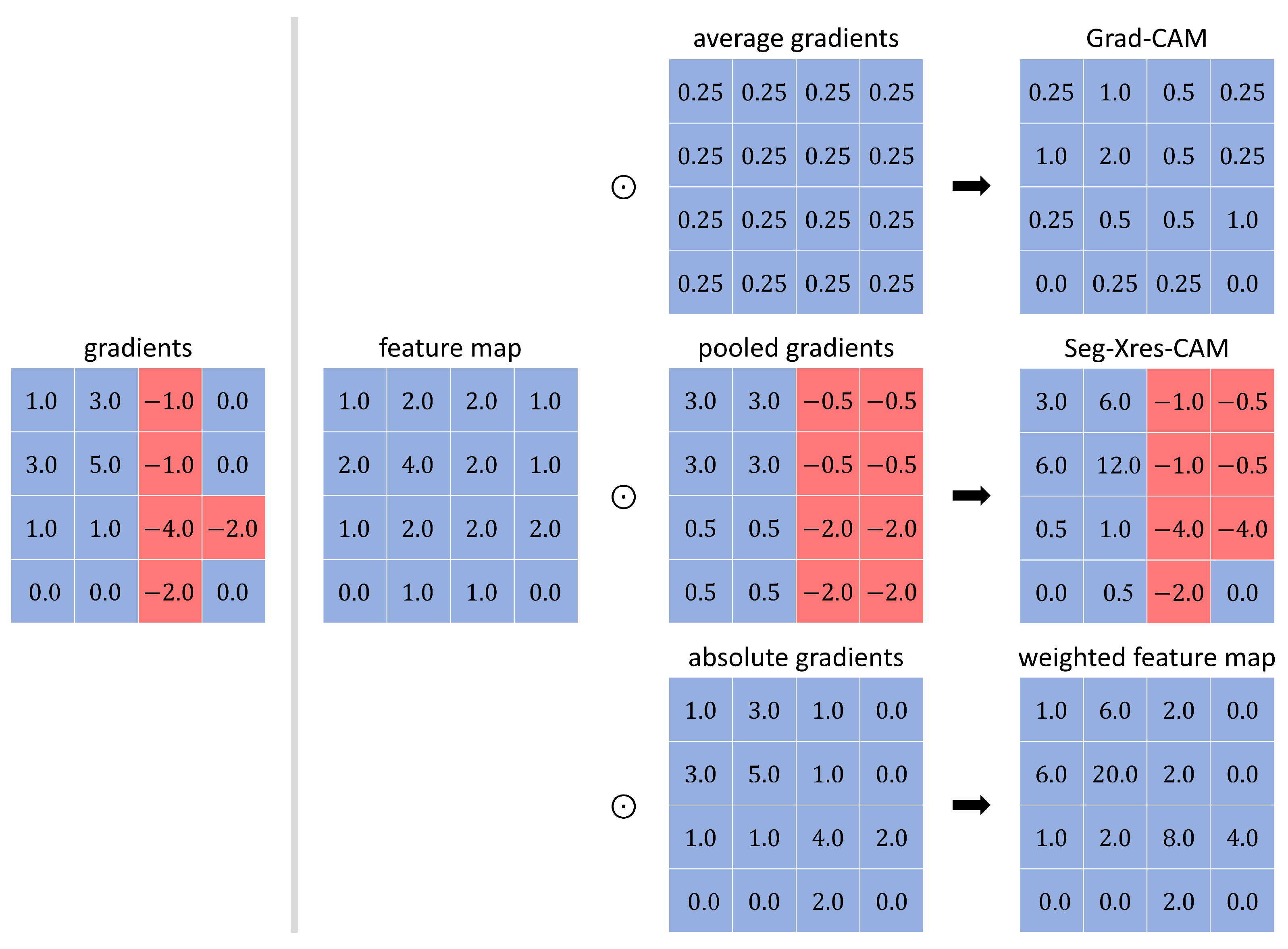
As shown in Figure 4, Grad-CAM emphasizes understanding which input features contribute most to the overall classification result, using the global average pooling of gradients to capture a global interpretation of features. In contrast, Seg-Xres-CAM adopts a local pooling approach, allowing it to capture the variations in the gradients within specific regions. Although this method preserves more spatial information, it may still introduce additional noise, particularly in edge regions, where larger gradient variations can lead to overestimating the influence of features near the boundaries, causing the activation of non-target areas to increase and affecting the accuracy of the visualizations. To address these limitations, we propose a method that focuses on gradient magnitude values, which not only reduces noise interference but also provides a more accurate quantification of feature importance. By multiplying absolute gradient values with activation maps, we obtain a weighted activation map with high spatial resolution that more faithfully represents pixel-wise contributions. For further analysis of this weighted activation map, we employ SVD in subsequent steps to extract key information.

3.2.2. Sign Correction Strategy

Next, our approach follows the same procedure as Eigen-CAM: we perform SVD on $O_{L=k}$ and extract its principal components, capturing the most significant variance in the feature activation. The localization map $L_{Ours}^c$ is then obtained by projecting $O_{L=k}$ onto the first principal component. The computation process is defined as follows:

$$O_{L=k}=U\mathsf{\Sigma }{V}^T$$

(11)

$$L_{Ours}^c=O_{L=k}{V}_1$$

(12)

However, a fundamental mathematical property of SVD results in the issue of sign ambiguity: When a matrix A is decomposed as $U\mathsf{\Sigma }{V}^T$, the column vectors of U and V can change signs simultaneously without affecting the final decomposition. This is because $\left(-1·U\right)·\left(-1·V^T\right)=U·V^T$. This phenomenon, known as sign ambiguity [21,22,23,24], poses challenges in feature extraction and visualization by potentially changing the representation of salient regions, thereby affecting the stability, consistency, and interpretability of feature maps.

To address this issue, we propose a Dynamic Sign Correction Mechanism as a post-processing step for the localization map. Specifically, we perform a directional analysis by comparing the absolute values of the extrema in the localization map, dynamically adjusting its overall sign. The correction mechanism is defined as follows:

$$L_{Ours}^c=\left\{\begin{array}{cc}\hfill L_{Ours}^c,& \mathrm{if}\left|max\left(L_{Ours}^c\right)\right|>\left|min\left(L_{Ours}^c\right)\right|,\hfill \\ -1·L_{Ours}^c,\hfill & \mathrm{otherwise}.\hfill \end{array}\right.$$

(13)

This mechanism is based on the optimization principle of feature representation, which assumes that in a well-optimized saliency map, class-discriminative information should contribute positively. When the absolute value of the negative extrema significantly exceeds that of the positive extrema, it often indicates a suboptimal assignment of signs. By dynamically correcting the sign, our method ensures that the primary feature information remains aligned with the positive direction, thereby enhancing the consistency and interpretability of the localization map. Furthermore, this correction strategy not only rectifies potential directional bias but also enhances feature representation stability through a simple linear transformation.

3.3. Evaluation Metrics and Performance Indicators

One of the key challenges in developing XAI methods for deep convolutional neural networks is how to objectively evaluate their effectiveness in a rigorous and standardized manner. A major difficulty in this process lies in determining appropriate evaluation metrics that can effectively measure the relevance, fidelity, and overall quality of an explanation.

To comprehensively assess the effectiveness of the proposed method, this study adopts the experimental framework established by Hasany et al. [19], using the relevance-based element retention approach as the primary evaluation strategy. The evaluation procedure follows a series of steps. First, the generated saliency map $L^c$ is binarized to retain only the highlighted regions, with the remaining areas masked out. Next, the resulting masked image $I^H$ is fed back into the model for prediction. Finally, the relevance of the explanation is measured by comparing the model predictions for the original image, denoted as Y, with those for the masked image, denoted as $Y^H$. The comparison is performed using the Dice score $Dic{e}^H$, which quantifies the similarity between the two sets of predictions. The computation process is defined as follows:

$$mas{k}_p=\left\{\begin{array}{cc}1,\hfill & \mathrm{if}{L}_p^c>\tau ,\hfill \\ 0,\hfill & \mathrm{otherwise}.\hfill \end{array}\right.$$

(14)

$$I^H=I\odot mask$$

(15)

$$Dic{e}^H={\displaystyle \frac{2·|Y\cap Y^H|}{\left|Y\right|+|Y^H|}}$$

(16)

Here, $mask$ represents the binarized mask, $p\in {\mathbb{R}}^{i\times j}$, and $\tau$ is the threshold to preserve the highlighted regions. In this study, we set $\tau =0$ to ensure the integrity of the highlighted regions, thereby preserving fine-grained details in the explanation results.

However, this study does not adopt the relevance-based element masking approach as an evaluation metric. This decision is based on experimental observations. When the saliency map exhibits high-intensity activations in the background, the highlighted regions tend to be excessively large. In such cases, extensive masking removes critical information required for the prediction, leading to prediction failures and causing the Dice score to approach zero. Although this metric can reveal the sensitivity of the model, when the masked area is too large, performance differences between explanation methods become less distinguishable, reducing the discriminatory power and effectiveness of the evaluation. In light of these considerations, this study chooses to exclude this metric in order to ensure the reliability of the evaluation results.

Recognizing the limitations of a single metric, this study proposes a novel metric of “Preserved Effectiveness” ($PE$), which integrates the Dice score with the proportion of retained salient regions ($RetainImage$), which is defined as follows:

$$RetainImage(\%)={\displaystyle \frac{{\sum }_{p}mas{k}_p}{{\sum }_{p}1}}\times 100$$

(17)

$$PE={\displaystyle \frac{Dic{e}^H}{RetainImage(\%)}}$$

(18)

This metric aims to balance the trade-off between effectiveness and efficiency in evaluating explanation methods. Specifically, an ideal saliency map should focus on regions that are most relevant to the model’s decision rather than irrelevant or distracting background regions. Although retaining larger salient regions may help maintain a higher Dice score, this approach often compromises the precision of the explanation. Thus, $PE$ serves as a comprehensive evaluation measure, incorporating the following key aspects:

• Relevance—An ideal explanation method should accurately identify the key regions that influence the prediction. The Dice score directly reflects whether the explanation method captures areas crucial to the decision-making process of the model.
• Low Complexity—A complex explanation incorporates all relevant regions to identify features critical for predictions. However, excessive complexity can diminish interpretability, even when the explanation faithfully represents the model’s behavior. $RetainImage$ metric quantifies this complexity by measuring the proportion of regions retained, providing an objective assessment of the explanation density.
• Synergistic Performance—This metric ensures that the evaluation measures operate in a complementary and synergistic manner, enabling explanations to precisely highlight critical regions while maintaining appropriate conciseness. This balance optimizes the overall effectiveness and improves the trustworthiness of the interpretations.

4. Experiments

To evaluate the effectiveness and robustness of the proposed Seg-Eigen-CAM method, we conducted extensive experiments on semantic segmentation models. This section presents comprehensive quantitative and qualitative analyses to assess the interpretability and stability of our approach. We begin by describing the experimental setup and evaluation protocols, followed by systematic ablation studies and quantitative comparative analyses with existing methods. In addition, we provide visual evaluations of local interpretability, qualitative assessments in complex scenarios, and detailed case studies to demonstrate the practical effectiveness of our method.

4.1. Datasets and Models

This study uses the val2017 subset of the COCO dataset (Common Objects in Context) [35]. This subset contains 5000 high-quality annotated images across 80 object categories, covering a diverse range of natural scene images. The variety in the image data provides a comprehensive and representative basis for evaluation.

The experimental framework in this study is based on OpenMMLab’s MMSegmentation [36] toolkit. This open source image segmentation toolkit is well regarded for its modular design, flexibility, and ease of use. It also utilizes pre-trained models trained on several public benchmark datasets, providing a solid technical foundation for our research. In the experiments, we selected three different semantic segmentation models: DeepLabV3 [24], PSPNet [37], and BiSeNetV1 [38]. All models employ ResNet-50 as the backbone network and are pre-trained on the COCO-Stuff 164K dataset. Detailed configuration parameters and performance comparisons for each model are shown in

Table 1. Experimental configurations and performance comparison of the models [36].

Model	Backbone	Crop Size	Lr schd	mIoU
DeepLabV3	R-50-D8	512 × 512	160,000	41.09
PSPNet	R-50-D8	512 × 512	160,000	39.64
BiSeNetV1	R-50-D32	512 × 512	160,000	34.88

. In all experiments, we extracted saliency maps from the model bottleneck.

4.2. Data Preprocessing

During the data preprocessing stage, we performed filtering and cleaning on the val2017 dataset. Initially, a preliminary inspection revealed that 48 of the 5000 images in the original dataset were unlabeled. To ensure data integrity and eliminate potential sources of bias, we removed these images, retaining a final set of 4952 images.

Next, for each image, we selected the annotated category that occupies the largest area of pixels as the target class. This decision was guided by several key considerations. Attempting to interpret all small objects within an image could lead to unreliable and less meaningful results. For instance, when a category occupies only a minimal pixel area, the region contains insufficient features, making it difficult for the model to learn effective discriminative information. Consequently, explanations for such regions are more susceptible to local noise, image compression artifacts, or annotation errors, which could cause discrepancies between the explanation and the actual predictive features. Furthermore, when the model explanation slightly expands or contracts such a region, evaluation metrics may exhibit nonlinear variations due to changes in pixel count, making it challenging to consistently assess the effectiveness of the explanation method. This could reduce the reliability of the metric values and potentially lead to misleading conclusions.

Finally, to ensure the reliability of the statistical analysis, we retained only categories with more than 40 samples. In this process, we removed 44 categories, accounting for 541 images, to prevent statistical bias due to insufficient sample sizes and to avoid extreme fluctuations in evaluation results that could compromise the trustworthiness of the overall experiment. After these filtering steps, the final dataset consisted of 4411 images. The distribution of target categories and their corresponding counts is summarized in

Table 2. Target category distribution statistics of the dataset.

Category	Counts	Category	Counts	Category	Counts
Person	1580	Cat	77	Chair	62
Car	109	Dog	62	Couch	83
Motorcycle	89	Horse	98	Bed	105
Airplane	83	Sheep	46	Dining Table	249
Bus	134	Cow	73	Toilet	102
Train	148	Elephant	83	TV	73
Truck	98	Bear	46	Laptop	54
Boat	83	Zebra	77	Oven	50
Traffic Light	45	Giraffe	91	Sink	59
Fire Hydrant	45	Umbrella	47	Refrigerator	58
Bench	86	Bowl	59	Clock	92
Bird	61	Pizza	54	Teddy Bear	50

.

4.3. Evaluation Framework

In XAI research, the effective and reliable evaluation of explanation methods remains a critical challenge. To address this issue, this study proposes a comprehensive multi-metric evaluation framework that assesses various explanation methods from multiple perspectives. The core evaluation strategy of this framework is the relevance-based element retention approach, which measures whether an explanation method can accurately identify and capture the crucial factors that influence model decisions. In addition, we introduce the Preserved Effectiveness as a complement to the Dice score. Unlike purely numerical performance metrics, $PE$ emphasizes both the precision and interpretability of the explanations, thus enhancing the credibility and practical value of the model interpretations.

Furthermore, this study incorporates the M3 metric proposed by Gizzini et al. [31] as a supplementary evaluation criterion. This metric evaluates the stability of explanation methods by analyzing the uncertainty of the prediction, providing an alternative perspective on the behavior of the model when key regions are preserved, which is defined as follows:

$$E\left(X\right)=\sum _{\forall p\in X}(-{\displaystyle \frac{1}{log\left(L\right)}}\sum _{l=1}^L{P}_X^{(p,l)}log(P_X^{(p,l)}))$$

(19)

$$E_{XAI}={\displaystyle \frac{E\left(I\right)-E\left(I^{\prime }\right)}{E\left(I\right)}}$$

(20)

Here, $E\left(X\right)$ represents the total pixel-level entropy of the input image X, $p\in {\mathbb{R}}^{i\times j}$, and $P_X^{(p,l)}$ denotes the softmax output of the model in the l-th feature map. $I^{\prime }$ refers to the masked image that retains only the salient and target regions.

In summary, this study evaluates explanation methods from multiple dimensions and adopts $Dic{e}^H$, $E_{XAI}$, and $PE$ as the primary metrics within the proposed multi-metric evaluation framework. These metrics provide an effective and reliable means to assess the performance of explanation methods.

4.4. Ablation Study

4.4.1. Gradient Weighting Strategy Experiments

In this section, we conduct an ablation study on gradient weighting strategies to compare different approaches and analyze their impact on model interpretability.

Table 3. Ablation study results of gradient weighting. The bold font number indicate the highest value corresponding to each label.

${\mathbf{Mean}\mathbf{Dice}}_{\mathit{H}}$
Label	${\mathbf{Strategy}}_{\mathbf{1}}$	${\mathbf{Strategy}}_{\mathbf{2}}$	Label	${\mathbf{Strategy}}_{\mathbf{1}}$	${\mathbf{Strategy}}_{\mathbf{2}}$
Person	0.82	0.81	Bear	0.58	0.58
Car	0.61	0.60	Zebra	0.84	0.84
Motorcycle	0.80	0.80	Giraffe	0.78	0.79
Airplane	0.65	0.66	Umbrella	0.69	0.69
Bus	0.69	0.69	Bowl	0.38	0.38
Train	0.69	0.70	Pizza	0.68	0.68
Truck	0.54	0.55	Chair	0.35	0.35
Boat	0.54	0.55	Couch	0.46	0.47
Traffic Light	0.53	0.54	Bed	0.56	0.55
Fire Hydrant	0.81	0.81	Dining Table	0.48	0.48
Bench	0.48	0.49	Toilet	0.79	0.78
Bird	0.55	0.55	TV	0.73	0.73
Person	0.82	0.81	Bear	0.58	0.58
Car	0.61	0.60	Zebra	0.84	0.84
Motorcycle	0.80	0.80	Giraffe	0.78	0.79
Airplane	0.65	0.66	Umbrella	0.69	0.69
Bus	0.69	0.69	Bowl	0.38	0.38
Train	0.69	0.70	Pizza	0.68	0.68
Truck	0.54	0.55	Chair	0.35	0.35
Boat	0.54	0.55	Couch	0.46	0.47
Traffic Light	0.53	0.54	Bed	0.56	0.55
Fire Hydrant	0.81	0.81	Dining Table	0.48	0.48
Bench	0.48	0.49	Toilet	0.79	0.78
Bird	0.55	0.55	TV	0.73	0.73
Cat	0.49	0.48	Laptop	0.66	0.67
Dog	0.67	0.66	Oven	0.53	0.56
Horse	0.69	0.70	Sink	0.53	0.54
Sheep	0.68	0.68	Refrigerator	0.60	0.61
Cow	0.58	0.58	Clock	0.67	0.66
Elephant	0.75	0.75	Teddy Bear	0.73	0.73

presents the detailed results of this experiment. Specifically, ${\mathbf{Strategy}}_1$ refers to multiplying the gradient by the activation map, while ${\mathbf{Strategy}}_2$ involves multiplying the absolute value of the gradient by the activation map. From the results in Table 3, we observe that both strategies yield comparable performance across most categories, indicating that our approach does not introduce a significant negative impact on the Dice score. However, in certain categories, ${\mathbf{Strategy}}_2$ slightly outperforms ${\mathbf{Strategy}}_1$ by ensuring a consistent directional input, thus emphasizing the numerical significance of the features. This suggests that ${\mathbf{Strategy}}_2$ may offer greater stability in certain feature recognition tasks.

In general, while the performance differences between the two strategies are relatively minor, we hypothesize that this may be attributed to the limitations of the evaluation metrics. Purely numerical assessments may not fully capture the characteristics and implications of different methods. To gain deeper insights into the interpretability advantages of our approach, we further explore this aspect in the subsequent qualitative analysis.

4.4.2. Sign Correction Strategy Experiments

In this section, we conduct an ablation study to analyze the effect of the sign correction strategy on the interpretability of the model.

Table 4. Ablation study results of sign correction. The bold font number indicate the highest value corresponding to each label.

${\mathbf{Mean}\mathbf{Dice}}_{\mathit{H}}$
Label	w/o Correction	w Correction	Label	w/o Correction	w Correction
Person	0.73	0.81	Bear	0.38	0.58
Car	0.40	0.60	Zebra	0.44	0.84
Motorcycle	0.48	0.80	Giraffe	0.46	0.79
Airplane	0.40	0.66	Umbrella	0.45	0.69
Bus	0.40	0.69	Bowl	0.25	0.38
Train	0.55	0.70	Pizza	0.51	0.68
Truck	0.39	0.55	Chair	0.23	0.35
Boat	0.30	0.55	Couch	0.44	0.47
Traffic Light	0.33	0.54	Bed	0.48	0.55
Fire Hydrant	0.51	0.81	Dining Table	0.54	0.48
Bench	0.27	0.49	Toilet	0.59	0.78
Bird	0.39	0.55	TV	0.51	0.73
Cat	0.39	0.48	Laptop	0.47	0.67
Dog	0.49	0.66	Oven	0.43	0.56
Horse	0.41	0.70	Sink	0.27	0.54
Sheep	0.40	0.68	Refrigerator	0.48	0.61
Cow	0.51	0.58	Clock	0.32	0.66
Elephant	0.52	0.75	Teddy Bear	0.46	0.73

presents the detailed results of this experiment. As shown in Figure 5, we select a scene image that contains both the target class (person) and various background regions for analysis. Without sign correction, the model exhibits a strong negative response in the target class region while displaying a weaker positive response in non-target background areas. This contradicts intuitive explanations. In contrast, after applying sign correction, the model’s attention is more effectively concentrated on the person, producing a visual explanation that aligns with human perception.

The experimental results indicate that, due to the inherent symbolic ambiguity in the feature space, uncorrected saliency maps may lead to instability and inconsistency in explanation results. Specifically, this can cause the model to overemphasize background regions while suppressing truly important areas. By incorporating the sign correction strategy, we successfully mitigate this issue, enabling the model to generate more stable and intuitive explanations.

4.4.3. Evaluation Metrics Experiments

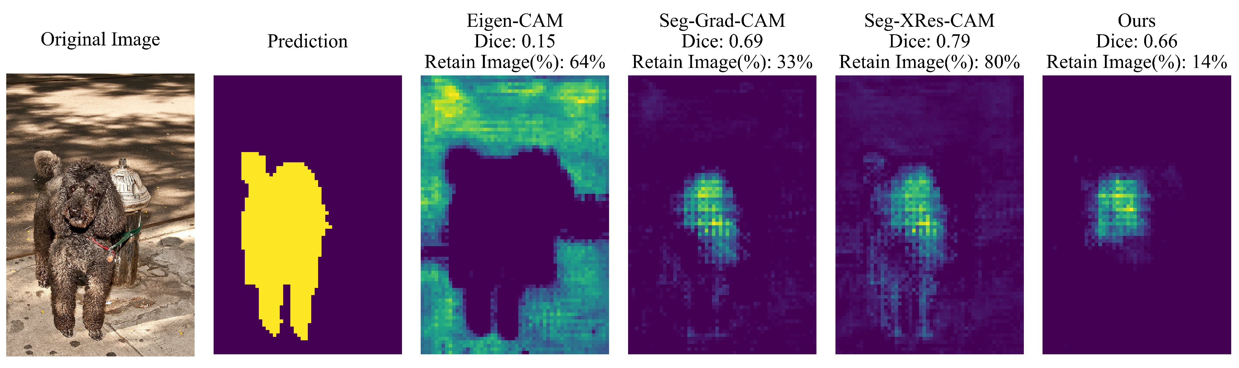
In this section, we conduct a case study to examine the reliability and interpretability of evaluation metrics. As shown in Figure 6, we analyze an image containing a single target class (dog). The experimental results indicate that although Seg-XRes-CAM achieves the highest Dice score (0.79), effectively preserving the overall contour of the target object, it also retains a substantial portion of the background. This phenomenon is reflected in its relatively high image retention rate. In contrast, both Seg-Grad-CAM and our proposed method focus primarily on the head region of the target object, aligning more closely with human visual perception. Although these methods yield a comparatively lower Dice score, their explanations are more precise and intuitively understandable. In particular, our approach demonstrates the highest interpretability by accurately localizing the key decision-influencing regions while maintaining the lowest image retention rate. Meanwhile, Seg-Grad-CAM retains some irrelevant background regions due to noise interference.

To further quantify the quality of the XAI method, we introduce the Preserved Effectiveness metric and compute the value $PE$ for each method: Eigen-CAM (0.23), Seg-Grad-CAM (2.09), Seg-XRes-CAM (0.99), and our proposed method (4.71). The results clearly demonstrate the superiority of our approach in terms of the quality of the explanation. The $PE$ metric effectively captures the spatial precision of the explanations, revealing the critical regions that influence the model decisions. A higher PE value indicates that the method provides a more refined and focused explanation, avoiding the inclusion of extensive background areas or weakly relevant regions, thus more accurately reflecting the core basis of the model’s decision-making process. This multidimensional evaluation framework mitigates the limitations of relying on a single metric, ensuring that the explanation results are both interpretable and reliable, ultimately enhancing their practical value.

4.5. Quantitative Analysis

In this section, we evaluate the effectiveness of various interpretability methods using a comprehensive evaluation framework to quantitatively assess their explanation performance. This framework enables a multidimensional evaluation of explanation capabilities, providing an in-depth analysis of the advantages and limitations of different methods.

Table 5. Comprehensive evaluation results of XAI methods. The bold font number indicate the highest value corresponding to each label.

Method	Model	Eigen-CAM	Seg-Grad-CAM	Seg-XRes-CAM	Ours
${\mathit{MeanDice}}_{\mathit{H}}$	DeepLabV3	0.49	0.75	0.80	0.69
	PSPNet	0.47	0.79	0.81	0.69
	BiSeNetV1	0.44	0.54	0.60	0.55
${\mathit{MeanE}}_{\mathit{XAI}}$	DeepLabV3	0.12	0.14	0.07	0.13
	PSPNet	0.17	0.28	0.23	0.31
	BiSeNetV1	0.11	0.15	0.17	0.10
Mean PE	DeepLabV3	1.19	1.88	1.19	5.34
	PSPNet	1.27	1.23	1.22	5.01
	BiSeNetV1	1.46	2.00	1.21	4.38

presents the results of the comprehensive evaluation of different explanation methods in three semantic segmentation models applied to all images in the dataset.

The experimental results indicate that Seg-XRes-CAM exhibits the best performance in ${Dice}_H$, achieving the highest scores in most categories in all three models. This demonstrates its ability to accurately capture the regions of interest influencing the model’s decision, effectively utilizing spatial information to generate local explanations. This results in high consistency and fidelity, with the attention regions aligning closely with the predicted regions. However, even less precise XAI methods often produce large highlighted areas in the image, which may overlap with the predicted regions, thus preventing extremely low ${Dice}_H$ scores. This phenomenon is observable in Eigen-CAM: although its explanations may not align with intuitive human judgments and may even be deemed incorrect, it still maintains a certain level of ${Dice}_H$. In addition, all methods perform poorly on BiSeNetV1 in terms of ${Dice}_H$, probably due to the lower baseline performance of BiSeNetV1 as a lightweight semantic segmentation model, as shown in Table 1. This highlights the impact of the performance of the underlying model on the explanation results.

For the $E_{XAI}$ metric, Seg-XRes-CAM and our proposed method demonstrate superior performance in individual class evaluations, with lower values of $E_{XAI}$. This suggests that these methods are more effective in identifying key features that influence the model’s segmentation decisions, excelling in local interpretability. However, our method also faces challenges: By retaining only the primary directional information in the image regions, some details may be overlooked. When the masked image is re-predicted, this may lead to prediction failure, with some classes exhibiting a higher increase in entropy. This phenomenon reflects the instability that can arise under low image retention rates, which also explains why our overall average performance is lower than Seg-XRes-CAM.

For the $PE$ metric, our proposed method outperforms all other methods in all models and classes. As shown in

Table 6. Image retention rate of XAI methods. The bold font number indicate the highest value corresponding to each label.

Method	Model	Eigen-CAM	Seg-Grad-CAM	Seg-XRes-CAM	Ours
Mean Retain Image (%)	DeepLabV3	50	46	69	18
	PSPNet	49	68	69	20
	BiSeNetV1	39	30	51	16

, our method achieves significantly lower image retention rates while maintaining stable performance ${Dice}_H$, demonstrating its ability to effectively identify the core decision-making regions. In contrast, Seg-XRes-CAM shows a higher ${Dice}_H$, indicating that it can faithfully present the rationale of the model decision. However, because the explanation is coarser and the influence of gradient weighting and gradient noise, Seg-XRes-CAM exhibits comparatively poorer performance in the $PE$ metric. Although Eigen-CAM $PE$ is similar to other methods, it is important to note that $PE$ can only effectively reflect the quality of the explanations when ${Dice}_H$ is sufficiently high.

To visualize the performance of each explanation method, we present the distribution of the Dice score and the image retention rate in a two-dimensional histogram, as shown in Figure 7. The analysis reveals that Eigen-CAM’s samples are concentrated in the bottom-left region, indicating suboptimal explanation performance. Gradient-based methods demonstrate higher image retention rates, with their high ${Dice}_H$ values indicating an effective representation of the model’s decision rationale. In comparison, samples from our proposed approach cluster in the bottom-right region, suggesting superior capability in identifying critical regions that influence model decisions while minimizing the impact of irrelevant areas. The distribution pattern in the two-dimensional plane demonstrates both the correlation and stability characteristics of each method, highlighting their respective reliability. Optimally, an attribution map should preserve maximum prediction information within a minimal image area; therefore, distributions closer to the bottom-right quadrant represent more effective explanation outcomes.

4.6. Performance of Local Interpretability

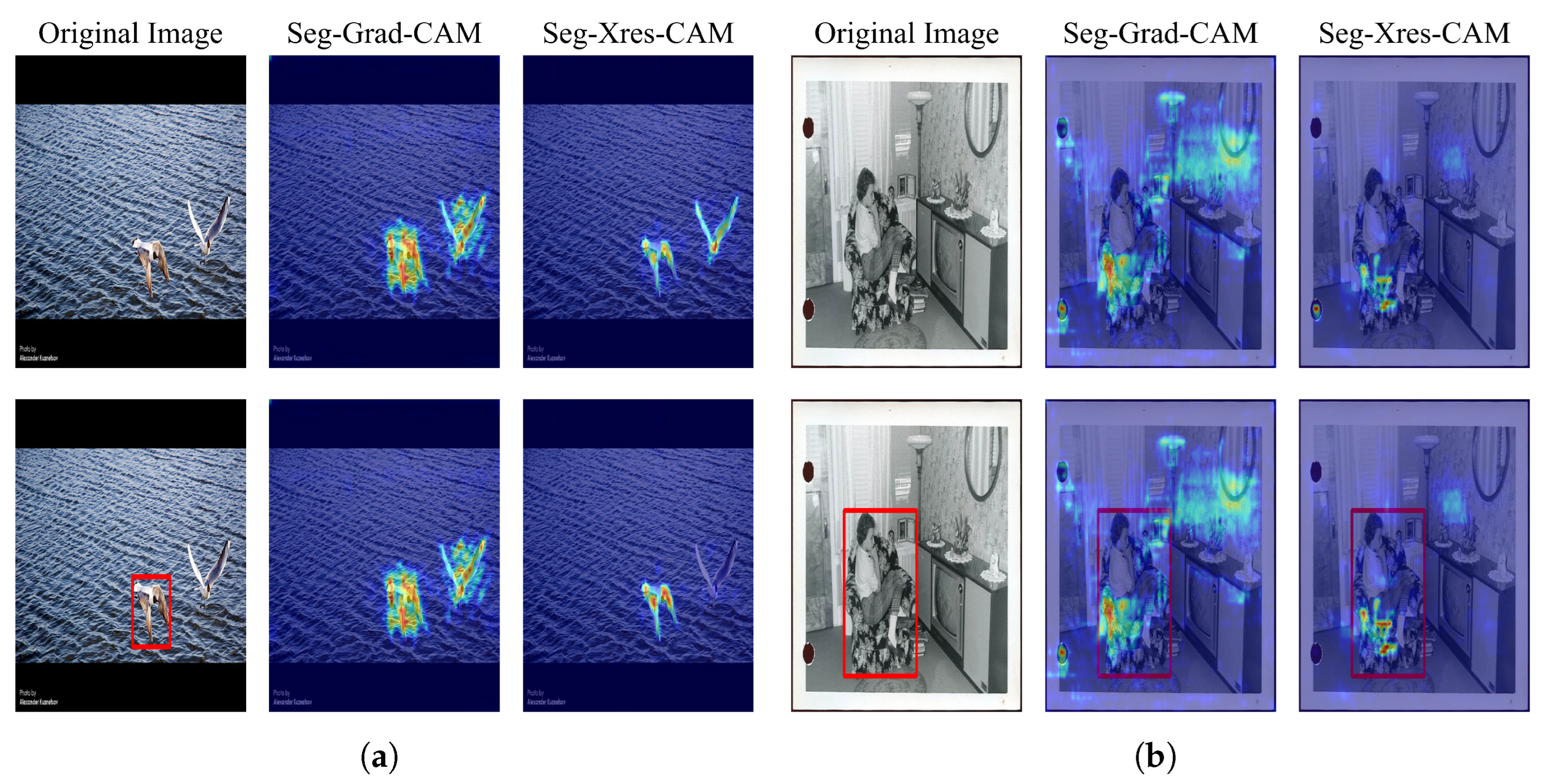
To evaluate the performance of different methods in generating localized explanations, we analyzed an image containing the target class (bird), as shown in Figure 8. Since Seg-Grad-CAM, Seg-XRes-CAM, and our method all employ similar mechanisms to focus on regions of interest, comparing their respective heatmap distributions allows us to directly assess their ability to preserve spatial information and accurately locate target objects.

From the figure, it is evident that Eigen-CAM and Seg-Grad-CAM struggle to accurately localize target regions because of their inability to fully incorporate the spatial information. As a result, their heatmaps display significant background interference, with strong activations appearing in non-target areas such as branches and leaves. In contrast, Seg-XRes-CAM and our method effectively leverage spatial information, allowing more precise identification and interpretation of the model focus areas. This advantage is particularly noticeable in multi-objective scenarios; for example, in the second example in Figure 8, both methods clearly highlight the location of the bird and generate the corresponding localized explanations.

The experimental results highlight the importance of retaining and utilizing spatial information when generating localized explanations. By effectively integrating spatial context with feature representations, our proposed method ultimately improved the precision and reliability of model explanations.

4.7. Performance in Complex Scenarios

To investigate how different methods perform in complex scenarios, we analyzed images containing multiple densely distributed instances of the same target category (person), as shown in Figure 9. The figure reveals notable issues with Seg-XRes-CAM. For example, in the first scene, weak positive responses appear along the edges of umbrellas and at the boundaries of the crowd, causing the activation regions (blue areas) to extend into non-target regions such as umbrellas and the ground. This validates our previous discussion, highlighting how local pooling mechanisms can overestimate the influence of features at boundaries, leading to excessive activation in irrelevant areas.

In contrast, our method achieves more accurate target localization. In the same scene, it clearly distinguishes between relevant and non-relevant regions, generating heatmaps with more concentrated activation regions primarily focused on the human figures. This indicates that our approach is capable of preserving semantic consistency even in visually cluttered environments. A similar trend is observed in the basketball court scene, where our method maintains robust identification performance even under lower image retention rates, effectively filtering out irrelevant visual information and producing more precise and concise explanations.

The experimental results confirm the importance of precise spatial information utilization in enhancing the interpretability of the model in complex scenes. Using a more refined feature processing approach, our method effectively mitigates background interference commonly observed in gradient-based methods and generates more detailed and reliable explanations.

4.8. Case Study and Limitation Analysis

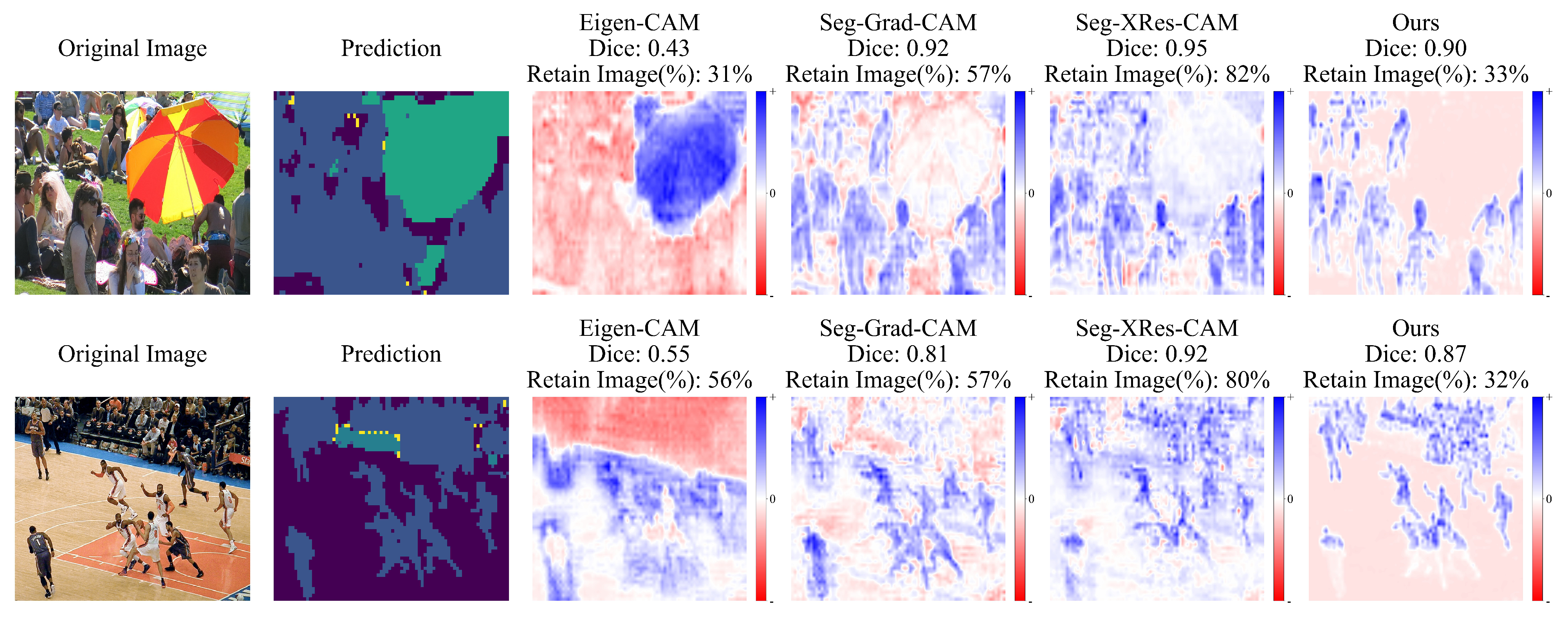
To further explore the potential limitations of evaluation metrics, this study selected several cases in which our method performed relatively poorly in quantitative metrics within images containing the target class (person). These cases help uncover biases and misconceptions that may arise from relying solely on quantitative metrics for evaluation.

As shown in Figure 10, in the first two scenes, although our method achieved relatively low Dice scores, the visual results reveal that Seg-Grad-CAM and Seg-XRes-CAM, despite achieving higher Dice scores, retained a larger retention of the image area. Specifically, Seg-XRes-CAM produced visual results similar to ours but retained a large amount of low-intensity responses in the background. This suggests that higher Dice scores may not necessarily reflect the quality of the explanation accurately. In the third scene, our method retained only 3% of the image area while still achieving a Dice score of 0.87. This further corroborates the fact that low-intensity responses generated by gradient-based methods may originate from gradient noise rather than key factors influencing the decision-making process of the model. Furthermore, in the fourth scene, our method not only identified the crowd in the stands but also accurately captured the head region of the players on the field. This aligns with the experimental conclusion in Section 4.4.3, showing that the model’s attention is typically focused on the head region of the target objects. This characteristic is consistent with the Human Visual System, indicating that the explanations generated by our method are more intuitive and interpretable.

However, these cases also highlight the limitations of relying solely on quantitative metrics for evaluation. When the pixel area of the target class is extremely small, even if the explanation effectively reflects the model’s decision-making process and aligns with human intuition, the limited features in that area may cause prediction failures when the masked image is re-predicted, leading to inaccurate conclusions from the evaluation metrics. Although evaluation metrics can assess the overall performance of XAI methods and provide insight into the characteristics of the method through 2D histograms, the black-box nature of deep learning models makes it difficult to accurately distinguish between errors in the model itself and biases in the attribution method. Therefore, relying solely on quantitative metrics to evaluate the quality of the explanation, especially in individual cases, can lead to erroneous conclusions.

To further investigate the explanation characteristics of different methods, we performed analyses in three cases with different scene characteristics, as shown in Figure 11. The experimental results demonstrate that our method exhibits a unique attention distribution pattern. Specifically, in the first scene, our method accurately captures the model’s focus on facial regions; in the second scene, it effectively highlights the hair regions; and in the third scene, it clearly delineates the subject’s edge contours. In contrast, while other methods achieved higher scores in evaluation metrics, their explanation contained substantial background regions that may be irrelevant to the decision-making process. This observation raises the crucial question of whether high evaluation metric scores truly reflect the actual effectiveness of explanation methods. Overly complex or coarse explanations may fail to accurately represent the model’s decision-making process, and it remains challenging to verify whether these non-target regions substantially influence the model’s decisions. Although our method generates explanations that align more closely with human visual perception and offer better interpretability, the inherent black-box nature of deep learning models prevents us from fully validating the faithfulness of these explanations.

5. Conclusions and Future Work

In this study, we have proposed an improved interpretability method for convolutional neural networks in semantic segmentation tasks. Building upon the Eigen-CAM framework, our approach incorporates spatial information and class-relevance scores from gradients, resulting in weighted activation maps that better capture region-specific attention. Furthermore, we introduced a dynamic sign correction mechanism to optimize feature representations derived from the singular value decomposition of weighted activation maps, effectively addressing the sign ambiguity issues that commonly arise in multi-class segmentation scenarios.

Our experimental results, comparing against established interpretability methods including Eigen-CAM, Seg-Grad-CAM, and Seg-XRes-CAM, demonstrate several significant findings. Although our method may not consistently outperform Seg-XRes-CAM in individual quantitative metrics, it exhibits superior performance in the Preserved Effectiveness metric. This high PE score substantiates that our method effectively identifies the critical regions necessary for class recognition without relying on complete target pixels or extensive background information. The method generates refined local explanations that align more closely with human visual perception, effectively highlighting object contours and key regions while filtering out low-relevance areas.

However, through a detailed qualitative analysis, we identified certain limitations in traditional evaluation metrics. Although our highly refined explanations may occasionally lead to prediction failures during re-prediction tests, they effectively reflect the model’s decision-making process. The visual results, while similar to Seg-XRes-CAM in some aspects, provide users with more concise and intuitive visual explanations, which is the core objective of interpretability methods.

Looking ahead, several promising research directions emerge from our findings. First, while our current dynamic sign correction mechanism effectively handles sign ambiguity, there is room for improvement in complex scenes. Future research could explore the integration of adaptive feature weight adjustment with multiscale feature analysis to enhance interpretation accuracy across varying target scales and scene complexities. Second, the method’s applicability could be extended to broader domains, such as medical image analysis and remote sensing, to evaluate its generalization capabilities comprehensively. Third, investigating the extensibility of the method to other deep learning architectures, including instance segmentation and object detection models, would validate its versatility.

A particularly crucial area for future work lies in developing more comprehensive evaluation frameworks. Given that the ultimate goal of interpretability methods is to provide intuitive and meaningful explanations to users, there is a need to establish human-centric evaluation standards. These standards should effectively assess how well the explanations aid human understanding and align with human visual cognition patterns. Such evaluation frameworks should combine both quantitative metrics and qualitative analyses to provide a more complete assessment of interpretability methods.