Abstract
In Global Navigation Satellite System (GNSS)-denied environments, opportunistic positioning using non-cooperative Low Earth Orbit (LEO) satellite signals has shown strong potential. However, dynamic platforms face challenges in maintaining sufficient satellite counts and favorable geometric distributions due to limited signal quality and short observation windows. To address this, we propose a fast satellite selection algorithm based on the Non-Dominated Sorting Whale Optimization Algorithm (NSWOA) for dynamic, multi-constellation LEO opportunistic navigation. By introducing Pareto non-dominated solutions, the algorithm balances Doppler Geometric Dilution of Precision (DGDOP), signal strength, residual visibility time, and receiver sensitivity. Through iterative optimization, it constructs a subset of satellites with minimal DGDOP while reducing computational burden, enabling real-time fusion and switching at the receiver end. We validate the algorithm through UAV-based experiments in dynamic scenarios. Compared to GWO, PSO, and NSGA-II, the proposed method achieves computation time reductions of 27.06%, 27.05%, and 68.57%, respectively. It also reduces the overall navigation solution time to 54.96% of that required when using all visible satellites, significantly enhancing real-time responsiveness and system robustness. These results demonstrate that the NSWOA-based satellite selection algorithm outperforms existing intelligent methods in both computational efficiency and optimization accuracy, making it well-suited for real-time, multi-constellation LEO dynamic opportunistic navigation.
1. Introduction
Low Earth Orbit (LEO) satellite systems provide key technical advantages—such as low latency, global coverage, high data rates, and anti-jamming resilience—which make them fundamental to next-generation satellite communication technologies [1,2,3]. The rapid deployment of mega-constellations like SpaceX’s Starlink has significantly accelerated global LEO satellite development. Systems such as Iridium, OneWeb, Kuiper, and China’s Xingwang are operational or in progress, and nearly 57,000 LEO satellites are expected to be in orbit by 2027 [4], providing multiple-layered global coverage and creating favorable conditions for high-precision opportunistic navigation using multi-constellation LEO satellite signals [5,6,7,8].
Constellation design advances have further improved spatial coverage and link quality. For instance, Guo et al. [9] proposed a piggyback-based deployment method to enhance scalability, while Cinelli et al. [10] developed a geometry-driven approach for optimizing inter-satellite visibility. Compared to traditional GNSS signals from Medium Earth Orbit (MEO) satellites, LEO downlink signals offer distinct advantages for Positioning, Navigation, and Timing (PNT), including enhanced frequency diversity [11,12,13], higher signal strength [14], and improved observation geometry [15,16]. These features have made LEO satellites a promising resource for resilient, GNSS-independent navigation systems, particularly under jamming or spoofing conditions [17,18,19,20].
LEO-based opportunistic PNT using non-cooperative signals has become a key area of research. Sun et al. [21] introduced a constant-vector thrust method for improved orbit control, laying the foundation for LEO-PNT in GNSS-denied environments. By analyzing frequency shifts in non-cooperative downlink signals, several studies have demonstrated the feasibility of low-accuracy PNT via pseudorange rate estimation [22,23,24,25]. Experimental results show that static platforms can achieve positioning accuracy within 5.1 m using signals from Starlink, OneWeb, Iridium NEXT, and Orbcomm satellites [26]. Complementary studies [27,28,29] have integrated inertial navigation with LEO Doppler measurements, confirming near-static performance on low-dynamic platforms. Theoretical simulations [28] have further explored real-time orbit estimation challenges for high-dynamic applications.
Moreover, link budget sensitivity has emerged as another critical factor in satellite selection. High-order modulation schemes can degrade link margins at low elevation angles [30], increasing the risk of signal loss. To address this, Di et al. [31] proposed a telemetry-aware node selection framework, and Höyhtyä et al. [32] designed a multi-layered communication architecture that improves resilience through cross-layer optimization. These developments suggest that future satellite selection strategies must account for both geometric precision and link stability in real-time applications.
Despite this progress, most research remains limited to static or low-dynamic conditions. Challenges such as rapid satellite motion, unknown ephemerides, and clock offset errors still hinder real-time use on dynamic platforms like UAVs [33]. Achieving an optimal balance between satellite geometry and computational efficiency is particularly difficult in dynamic environments, where satellite visibility is short-lived and time-constrained.
To overcome the spatiotemporal constraints of dynamic LEO satellite-based opportunistic navigation, this paper proposes a multi-objective satellite selection model using a swarm intelligence optimization algorithm—the Non-Dominated Sorting Whale Optimization Algorithm (NSWOA). The model integrates opportunity signals from multiple LEO satellite constellations under dynamic conditions. By tracking and predicting satellite motion trajectories, it comprehensively considers factors such as Doppler geometric precision, signal strength, remaining visibility time, observation elevation angle, and receiver sensitivity. This multi-attribute optimization facilitates satellite selection, enabling the receiving terminal to dynamically and automatically fuse and switch signals based on satellite cognition. Consequently, the approach iteratively updates the solution by determining a guiding agent and archiving non-dominated solutions, ultimately identifying the satellite combination with the minimum DGDOP and the fewest satellites. This enables an optimal balance between satellite geometry and computational load under dynamic conditions.
In our study, a dynamic application scenario is established to integrate observations from the Iridium, Iridium NEXT, Orbcomm, and Starlink constellations. A comparative analysis of satellite selection results is conducted using various optimization algorithms for multi-attribute decision-making. The results demonstrate that the NSWOA-based multi-attribute decision-making algorithm outperformed other methods in terms of optimization accuracy and computational efficiency. Building on this, a range-based positioning experiment using Doppler shifts from LEO satellite signals is conducted. The results show that the real-time performance and robustness of the navigation and positioning system based on the multi-attribute optimization satellite selection algorithm were significantly superior to conventional LEO satellite-based opportunistic navigation methods. Therefore, the proposed NSWOA-based multi-attribute satellite selection algorithm effectively enhances the real-time performance and robustness of multi-constellation LEO satellite-based dynamic opportunistic navigation.
2. Methods
2.1. Multi-Objective Optimization of the Satellite Selection Problem
Compared to MEO satellites, LEO satellites have a smaller ground coverage area, higher tangential velocity, and shorter observable durations, typically ranging from 4 to 10 min. These characteristics lead to a higher frequency of satellite switching in the visible field as the elevation angle changes. Therefore, in non-cooperative multi-constellation LEO satellite dynamic opportunistic navigation, the satellite selection algorithm plays a critical role.
To meet the real-time and continuous opportunistic navigation needs of dynamic users, the satellite selection algorithm for multi-constellation LEO dynamic opportunistic navigation must balance two key objectives. First, it should maximize the number of LEO satellites selected to improve positioning accuracy. Second, it must minimize the number of satellites involved in calculations to reduce the computational burden on the user’s receiver and enhance real-time positioning performance. These two objectives are inherently conflicting and subject to various constraints, such as ground signal power and the duration of observable satellite time.
To achieve an optimal balance, an efficient and well-structured multi-objective optimization algorithm is essential for refining the satellite selection strategy. Consequently, the process of selecting satellites for multi-constellation LEO dynamic opportunistic navigation can be modeled as a low-complexity multi-objective optimization problem.
In this study, the DGDOP value is chosen as one of the optimization objectives to evaluate the quality of the satellite geometric configuration, thereby reflecting its impact on positioning accuracy. The state equation of the dynamic opportunistic navigation model is similar to that of conventional GNSS/IMU tight coupling, but its observation equation differs. In dynamic opportunistic navigation, Doppler frequency shifts result from tracking the downlink beacon signals of LEO satellites. Moreover, LEO satellites from different constellations operate on distinct time systems, with each satellite providing only a single Doppler shift measurement per time update.
Let the discrete sampling time of the receiver at epoch represent the arrival time of the reference signal at , with as the initial time and as the sampling clock period. The signal transmission time of the LEO satellite at epoch is represented as , where represents the true propagation delay from the -th LEO satellite to the receiver. At epoch k, the Doppler frequency shift extracted from the signal of the -th LEO satellite is , while the pseudorange rate is , the beacon carrier frequency of the -th satellite is , and is the speed of light. represents the three-dimensional position vector of the dynamic platform at epoch k, denotes the three-dimensional position vector of the -th LEO satellite at epoch k’, and indicates the observed velocity of the dynamic platform at epoch k. The velocity of the l-th LEO satellite at epoch k’ is denoted as . Additionally, represents the clock drift error of the LEO receiver at epoch k, while denotes the clock drift error of the -th LEO satellite at epoch k’. is the total number of visible LEO satellites within the receiver’s field of view, and is the noise in the pseudorange rate, which is assumed to follow a normal distribution as additive noise. Due to the non-cooperative approach employed to extract Doppler frequency from LEO satellite signals, a clock drift error exists between the receiver and the LEO satellite. Based on the characteristics of LEO satellite clock drift referenced in the literature, the drift error between the receiver clock and the LEO satellite clock is modeled using linear fitting, represented as .The derivation based on the pseudorange rate obtained from observing the signal of the -th LEO satellite at epoch is given as follows [34]:
After linearizing Equation (1) and taking the partial derivatives with respect to the receiver state and clock bias, the observation equation can be expressed as follows:
The vectorized observation equation for the LEO satellites can be formulated as follows:
where represents the Doppler frequency error vector observed by the dynamic platform receiver from LEO satellites at epoch . denotes the gradient vector of the Doppler frequency observations in the spatial direction; represents the gradient vector of the Doppler frequency observations in the velocity direction; and indicates the gradient vector of the Doppler frequency observations in the time direction. By linearizing observation Equation (3), we can derive the following relationships: represents the positioning error; denotes the speed measurement error; indicates the clock drift error of the -th observed satellite relative to the receiver’s clock; and reflects the linearization error at epoch along with various types of additive measurement noise.
From the observation equation of dynamic opportunistic navigation using LEO satellites, the dynamic Doppler geometric dilution of precision (DGDOP) can be expressed as follows:
The positioning error can be expressed as the product of the user receiver’s Doppler measurement error and the Doppler geometric dilution of precision (DGDOP):
The number of satellites, , is considered another optimization objective, reflecting the computational burden on the user’s receiver. To balance multiple objectives, we introduce the concept of Pareto non-dominated solutions [35]. A solution is considered optimal and Pareto non-dominated if it outperforms (dominates) another solution if and only if it shows equal or better objective values across all objectives and provides a better value in at least one objective function. The selected set of satellites serves as agents evolving in search of multi-objective optimization, seeking to find the global Pareto non-dominated solution set. Thus, the multi-objective satellite selection problem can be formulated as follows:
where represents the decision vector for the search agents, is the size of the search agents, and is the objective vector function indicating the objective fitness. Here, reflects the fitness function related to positioning accuracy, while represents the fitness function concerning computational burden. The space refers to the decision space for satellite selection, and denotes the set of visible satellites within the observation field of the user’s receiver during a specific time period. Each represents a satellite carrying pseudo-random noise and is identified by its number . The function reflects the inequality constraint space related to ground signal power, while denotes the sensitivity of the user’s receiver. The function represents the inequality constraint space regarding the remaining observation time of the satellites within the field of view.
2.2. Design of the NSWOA Satellite Selection Algorithm
2.2.1. Whale Optimization Algorithm
According to the multi-objective optimization satellite selection model presented in Equation (6), the target fitness function reflecting positioning accuracy is given by , which corresponds to the DGDOP for observing non-cooperative LEO satellites. The target fitness reflecting the computational burden is expressed as , where denotes the number of selected satellites.
To determine the Pareto optimal front of the objective vector function , the Whale Optimization Algorithm (WOA) fixes the number of selected satellites (objective ) and classifies the fitness values (DGDOP) of the satellite combinations. The best DGDOP configuration is designated as the search guiding agent , while the remaining candidate combinations are treated as search agents . After establishing the fitness values and identifying the guiding agent, the algorithm employs the contraction and encirclement mechanism of the WOA’s bubble-net feeding behavior during the predation phase, combined with a spiral position updating model. The algorithm then iteratively updates the satellite search agents with equal probability, calculates the fitness of the updated , and subsequently updates the guiding agent . This process is repeated until the termination condition is satisfied, ultimately yielding as the Pareto non-dominated satellite combination, identified by . The solution thus represents the final desired satellite combination.
The WOA [36] algorithm simulates the hunting behavior of humpback whale populations in nature, dividing the process into three stages: prey searching, prey encircling, and bubble-net feeding.
The prey searching phase, also known as the exploration phase, involves randomly selecting a search agent as the reference agent to update the positions of other search agents. The process of prey searching is described as follows:
In Equation (7), denotes the iteration count, while represents the position vector of a randomly selected search agent and corresponds to the position vectors of the remaining search agents. The parameter is a convergence factor that linearly decreases from 2 to 0 as iterations progress. Additionally, and are randomly generated values within the range [0, 1].
In the encircling prey phase, the WOA sets the current best search agent as the target prey position, or the best solution closest to the target prey. Once the best search agent is defined, the other search agents update their positions in the direction of the best search agent, iteratively determining the optimal solution .
The bubble-net foraging phase, also known as the exploration phase, updates the whale’s position by probabilistically selecting between the shrinking encircling mechanism and the spiral position update model with equal probability, as expressed by
where represents a random number uniformly distributed in the interval [−1, 1] and is a constant that defines the logarithmic shape.
2.2.2. Archiving and Guiding Selection Mechanism
Building on the proposed mathematical definitions of optimal Pareto non-dominated solutions, a fast satellite selection algorithm—NSWOA—is developed. This algorithm incorporates two key innovations that enhance the original WOA for multi-objective optimization problems:
- An archiving mechanism, which maintains a dynamic set of non-dominated solutions during the optimization process;
- A guiding selection mechanism, which adaptively selects leading agents to balance convergence and diversity in the solution space.
These enhancements improve WOA and enable effective solution comparison in the multi-objective optimization satellite selection problem.
The archiving mechanism is designed to store the non-dominated Pareto optimal solutions generated during the optimization process. It regulates the inclusion of new satellite combinations in the archive while enabling the retrieval of existing non-dominated solutions. When a new satellite combination is evaluated, one of two possible outcomes occurs:
- Scenario A: If the new satellite combination dominates one or more existing solutions in the archive, the dominated solutions are removed, and the new combination is added.
- Scenario B: If the new combination is non-dominated relative to the existing solutions, it is simply added to the archive.
The selection mechanism in NSWOA is based on Pareto dominance, addressing the challenge of ranking multi-objective solutions using scalar fitness values alone. It selects guiding agents from the current archive of non-dominated solutions to steer the search process toward optimal satellite combinations. This mechanism operates in three main phases:
- Phase 1: Archive Space Partitioning
- Based on the maximum and minimum values in both and directions within the archive space, and using the adjustment factor , the partitioning ranges are determined as follows:. These ranges are specifically defined as follows:
- Then, both the and directions are uniformly divided into cells.
- Phase 2: Grid Congestion Probability Calculation
- The congestion probability for each grid is defined as follows:where is the number of Pareto optimal solutions in the -th grid, and is the guiding selection pressure parameter, typically set to . The probabilities are then normalized.
- Phase 3: Guiding Agent Selection
- The cumulative probability for the -th grid is calculated as follows:
The first grid index is identified such that , where is a random probability uniformly distributed within the range [0, 1].
- From the selected grid, a non-dominated agent is randomly chosen as the guiding agent .
This probability-biased selection method favors grids with lower solution density, thereby promoting exploration in less-crowded regions of the solution space and enhancing global search capability.
2.3. Procedure of the NSWOA-Based Satellite Selection Algorithm
As indicated by Equation (6), the decision space for the satellite selection strategy within the observational field for positioning is denoted as . In this context, the NSWOA, which incorporates both archiving and guiding selection mechanisms, selects a set of Pareto non-dominated satellite combinations from the decision space . The resulting set of Pareto non-dominated satellite combination agents is denoted as , where and represents the selection of LEO satellites. The steps of the NSWOA rapid satellite selection algorithm are shown in Table 1. The flow of the NSWOA rapid satellite selection algorithm is illustrated in Figure 1. The pseudocode for the satellite selection algorithm is presented in Table 2. The initial phase involves data preprocessing, during which visible satellites are identified and a viable satellite selection strategy space is generated. This process utilizes satellite IDs, downlink signal power, and orbital information derived from Two-Line Element (TLE) data. Satellites are considered visible if they meet two criteria: a remaining observable time greater than zero and a signal power exceeding the receiver’s sensitivity threshold.

Table 1.
Steps of the NSWOA rapid satellite selection algorithm.
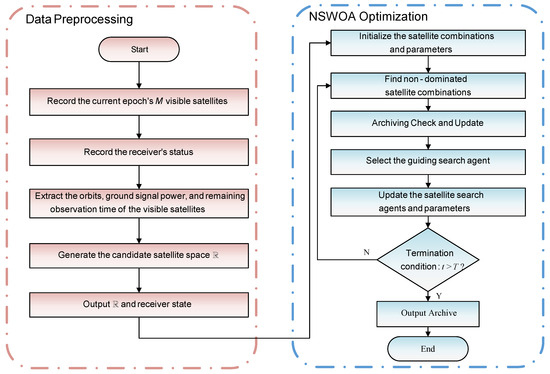
Figure 1.
Workflow of the NSWOA Fast Satellite Selection Algorithm for Dynamic Opportunistic Navigation with LEO Satellites.
Table 2.
Pseudocode of the satellite selection algorithm.
The selection module begins by initializing the satellite search agents and the associated parameters based on the input data, the specified agent population size , and the number of iterations T. The objective fitness values of the satellite search agents are then calculated. Non-dominated satellite combinations are updated in the archive, and the guiding search agent is identified from the archive. Subsequently, the satellite search agents and parameters are updated according to Equations (7) and (8), followed by boundary adjustments for the updated satellite search agent .
The iterative process continues until the specified number of iterations is reached. Finally, the archive is output, and the non-dominated Pareto satellite combinations contained in the archive are identified as the selected optimal satellite combinations.
3. Results
3.1. Experimental Conditions and Parameters
Satellite motion was predicted using TLE data in conjunction with the SGP4 model for three representative LEO constellations—Iridium, Orbcomm, and Starlink—encompassing a total of 6251 satellites. This method provides accurate short-term orbital predictions.
Doppler measurement noise is modeled as zero-mean Gaussian white noise with a fixed variance of 100 Hz2, a widely adopted and simplified assumption in signal processing. To simulate realistic observations, Doppler shifts are generated by superimposing the theoretical values with the noise.
The downlink coverage of each constellation was represented by specific depression angle ranges: 40°–90° for Starlink, 15°–90° for Iridium, and 20°–90° for Orbcomm. A minimum elevation angle of 30° is set for the receiver antenna to ensure visibility within the defined coverage constraints.
The signal power constraint in Equation (6) is expressed as , where the receiver sensitivity () is set to −140 dBW. Considering the actual Iridium signal transmission intervals and the required processing length for satellite signals, the remaining observable time is denoted by .
The UAV flight scenario is illustrated in Figure 2, where the trajectories of visible satellites are shown. A total of 2185 epochs, with a 30 s interval, were selected for the experiments. Initially, 20 Starlink satellites and 1 Orbcomm satellite were observed. After 228 s, an Iridium satellite entered the observation horizon. During the UAV flight in the scenario with 6251 satellites, an average of 22 LEO satellites were observed per second. The simulation was conducted on a computer with the following configuration: CPU: i7-12700F; Memory: DDR4-3200, 12 GB. Details of the simulation scenario and parameter settings are summarized in Table 3.
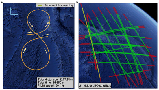
Figure 2.
Unmanned aerial vehicle simulation scenario. (a) Flight trajectory: A UAV, cruising at approximately 50 m/s, flew over a coastal region in Asia for 65,550 s, covering 3277.5 km. The trajectory included a straight climb to 1500 m, followed by an “8”-shaped cruising maneuver, and a descent back to 1000 m. (b) The trajectories of satellites: The visible Starlink and Orbcomm satellites are shown by green and yellow solid lines, respectively, while the red line represents the trajectory of the satellite as it moves out of the observable range.
Table 3.
Dynamic scenario parameters.
To evaluate the performance of the dynamic satellite selection algorithm in a UAV dynamic scenario, the proposed NSWOA satellite selection algorithm is compared with the Non-Dominated Sorting Genetic Algorithm II (NSGA-II) [37], Particle Swarm Optimization (PSO) [38], and Gray Wolf Optimization (GWO) [39] algorithms under identical conditions. Among them, PSO and GWO share a similar population-based framework with NSWOA. PSO and GWO are computationally efficient with few parameters, making them suitable for embedded or edge devices. In contrast, NSGA-II, though more complex, provides high-quality solutions through its non-dominated sorting mechanism and serves as a performance benchmark. These three algorithms collectively represent a balance between optimization quality and computational efficiency. For each algorithm, the initial satellite subset x consists of 200 search agents, and the number of iterations T is set to 100.
The parameters of the NSWOA are provided in Table 4. In comparison, NSGA-II has a crossover probability of and a mutation probability of . The PSO algorithm follows the NSWOA parameter settings, with a social learning factor of , a personal learning factor of , and an inertia weight defined as , where the maximum inertia weight is and the minimum inertia weight is . The GWO algorithm uses the same parameter settings as the NSWOA.
Table 4.
NSWOA parameters.
3.2. Dynamic Satellite Number Selection Experiment
Based on the experimental conditions, we conducted simulation experiments comparing dynamic satellite selection in the environment shown in Figure 2. Figure 3 presents a comparison of the average dynamic satellite selection outcomes and their corresponding DGDOP values over the UAV’s full flight trajectory, alongside the Pareto optimal frontier. The results demonstrate how closely the selection algorithms approach the theoretical performance limits. The DGDOP values optimized by the GWO algorithm are slightly higher than those of the other algorithms when the number of selected satellites is 6 or 7. The PSO algorithm generally performs worse than the NSWOA and NSGAII algorithms, with both NSWOA and NSGAII algorithms being closer to the theoretical frontier. When the number of selected satellites is less than 8, the DGDOP value of the NSWOA is lower than that of NSGAII, with an average reduction of 1.9136. However, when the number of selected satellites is between 8 and 10, the proposed NSWOA outperforms NSGA-II, with an average reduction of 0.5881. Moreover, NSWOA also outperforms the GWO and PSO algorithms, with the average DGDOP value decreasing by 2.0521. Table 5 summarizes the execution times of the compared algorithms. The proposed NSWOA achieves computation time reductions of 27.06%, 27.05%, and 68.57% compared to GWO, PSO, and NSGA-II, respectively. These results indicate that NSWOA not only yields solutions closer to the theoretical optimum but also demonstrates significantly improved computational efficiency. This advantage makes it particularly well-suited for real-time satellite selection in UAV-based applications.
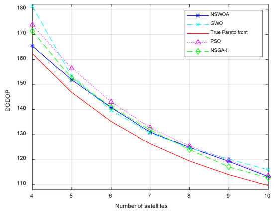
Figure 3.
Comparison of DGDOP between NSWOA, NSGA-II, PSO, and GWO algorithms. The true Pareto front refers to the fully ideal front obtained by exhaustively evaluating the DGDOP values of all possible satellite combinations.
Table 5.
Execution time per epoch (unit: seconds).
To evaluate the performance of multi-objective satellite selection algorithms, the Inverted Generational Distance (IGD) metric is used. IGD measures both the convergence and diversity of the solution set. It calculates the average distance from each point in a reference Pareto-optimal front to the nearest solution produced by the algorithm. A lower IGD value means that the solutions are close to the true Pareto front (good convergence) and well distributed along it (good diversity). In this way, IGD penalizes both inaccuracy and poor coverage. The IGD is calculated as follows:
In Equation (12), denotes the number of theoretical Pareto optimal solutions in the satellite combination reference set, and represents the Euclidean distance between the theoretical Pareto optimal solution of the -th satellite combination in the reference set and the nearest Pareto optimal solution obtained by the optimization algorithm. In the IGD metric, the Euclidean distance quantifies how close the theoretical satellite combination solution is to the nearest Pareto optimal solution in the algorithm’s objective space. The IGD values for the optimization results of different algorithms across the entire 2185 epochs of the UAV flight are computed. The boxplot and statistical results for the different performance metrics are shown in Figure 4.
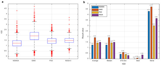
Figure 4.
The IGD results of the dynamic scene satellite selection algorithm over 2185 epochs. (a) Boxplot of IGD values: In the box plot, the red line represents the median, while the upper and lower edges of the box correspond to the first and third quartiles of the IGD values. The height of the box reflects the interquartile range (IQR). The whiskers extend to 1.5 times the IQR, and red plus signs indicate outliers beyond the whiskers. (b) Statistical results of IGD values: The comparison of algorithms is based on the average, median, standard deviation, best, and worst IGD values. The height of the histogram bars represents the magnitude of these metrics.
From the comparison in Figure 4, it can be observed that the box for the NSWOA is positioned lower, indicating smaller values, with better median and optimal values. The overall shape of the box is flatter, suggesting good convergence and diversity. The minimum IGD value for the NSWOA is 0.01, outperforming the GWO and NSGA-II algorithms and performing similarly to the PSO algorithm. In terms of average and median IGD values, the NSWOA surpasses the GWO, PSO, and NSGA-II algorithms by approximately 35%, 14%, and 17%, respectively. Moreover, it remains highly competitive in terms of standard deviation and worst-case values, demonstrating that the NSWOA possesses the best overall optimization capability.
The experimental results presented in Figure 3 and Figure 4 further confirm that the proposed NSWOA satellite selection algorithm produces solutions that are closer to the theoretical Pareto front. The algorithm demonstrates superior convergence and diversity throughout the entire flight and within a given satellite count range , the overall optimization performance of the proposed NSWOA still outperforms the other algorithms.
3.3. Fixed Satellite Selection Experiment
For dynamic users, the expected positioning accuracy permits the use of a fixed-number satellite selection strategy, simplifying the problem from multi-objective to single-objective optimization. At each epoch, five satellites are selected—four to satisfy the minimum navigation requirement (position and clock bias estimation) and one additional satellite to enhance geometric distribution. This approach also ensures manageable computational and data overhead, making it suitable for deployment on large unmanned aerial vehicles.
As shown in Equation (6), the goal is to minimize to determine the minimum DGDOP value. The iterative characteristics of the DGDOP within the observation epochs of the unmanned aerial vehicle’s flight trajectory are shown in Figure 5a, and the variation of the DGDOP values across the epochs is illustrated in Figure 5b.
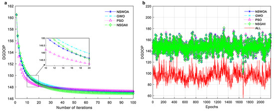
Figure 5.
Fixed number of satellites selection algorithm comparison. (a) Comparison of average DGDOP iterative changes across different algorithms throughout the entire flight. (b) Comparison of DGDOP across different algorithms and all satellite selections at each observation epoch.
Figure 5 illustrates the iteration results and the DGDOP convergence of each satellite selection algorithm. It can be observed that the DGDOP values in the observation epochs converge rapidly when the proposed NSWOA is applied. The iteration statistics are shown in Table 6.
Table 6.
Minimum iteration count corresponding to DGDOP results (unit: iterations).
As shown in Figure 5a and Table 6, the minimum number of iterations required by the NSWOA to achieve a DGDOP value below 150 is 11, which is two and one fewer than the iterations required by the GWO and NSGA-II algorithms, respectively. When the DGDOP value is reduced to below 148, the NSWOA still requires four fewer iterations than GWO but exceeds PSO and NSGA-II by four and five iterations, respectively. Further iteration to a DGDOP value below 147.5 results in NSWOA matching the performance of GWO, outperforming PSO, but falling short of NSGA-II. Based on this analysis, it can be concluded that when computational resources are limited and fewer iterations are allowed, the NSWOA converges faster than the GWO and NSGA-II algorithms. As the optimization target (DGDOP) decreases, the required number of iterations increases. However, NSWOA still exhibits faster convergence than GWO, eventually surpassing PSO. Overall, the NSWOA optimization algorithm demonstrates strong performance in the fixed satellite selection dynamic scenario.
Figure 5b shows that the DGDOP values optimized by each algorithm in the fixed satellite selection dynamic scenario are generally within the same range throughout the entire flight process. A more detailed statistical analysis is provided in Table 7.
Table 7.
DGDOP result statistics for 2,185 epochs across different algorithms.
The results shown in Figure 5b and Table 7 indicate that, in the single-objective fixed satellite selection dynamic scenario with 2,185 observation epochs, the proposed NSWOA demonstrates strong competitiveness. The percentage of epochs with DGDOP values between 130 and 170 is lower than that of GWO and NSGA-II, but overall higher than PSO, suggesting that NSWOA maintains good precision compared to classical algorithms. Although it slightly lags behind GWO and NSGA-II, the difference is within 1%. Furthermore, for epochs with DGDOP values greater than 180, the number of such epochs is fewer than those of NSGA-II and PSO, indicating that NSWOA maintains good optimization precision in most epochs and can still perform excellently in cases of occasional degradation.
Under conditions where dynamic user computational resources are limited and a fixed satellite selection strategy is employed, the NSWOA can still meet the dynamic satellite selection requirements in terms of both optimization results and speed.
3.4. Dynamic Opportunistic Navigation Experiment
Using the proposed NSWOA satellite selection algorithm and the multi-constellation LEO satellite dynamic opportunistic navigation models described in Equations (1) and (2), a positioning experiment was conducted with Starlink, Orbcomm, and Iridium satellites, as shown in Figure 2. The receiver coordinates were estimated using the least squares method by minimizing the residuals between the measured and theoretical Doppler shifts, thereby obtaining the solution that best fits the observation data. As indicated by Equation (5), the primary factors influencing positioning error in this study are the Doppler measurement error and the DGDOP value of the selected satellite combination. Accordingly, a navigation threshold of was applied, and the corresponding satellite selection results are shown in Figure 6. As illustrated, the NSWOA-based selection algorithm demonstrates high accuracy and strong autonomy under this constraint. The statistical data for the 2185 epochs of the algorithm are presented in Table 8. From Table 8, it can be observed that the DGDOP values obtained using the NSWOA are all below 150 for every epoch, indicating that the method meets the preset threshold requirements. Therefore, under reasonable threshold conditions, the proposed algorithm exhibits high accuracy, high automation, and broad applicability. The positioning results based on this satellite selection are shown in Figure 7.
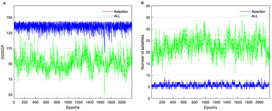
Figure 6.
Comparison of DGDOP and the number of satellites selected by all selection and the NSWOA Optimization. (a) Comparison of DGDOP values between NSWOA star selection results and all selection results. (b) The comparison of the satellite count between the NSWOA-selected subset and the all-satellite selection results.
Table 8.
Statistical results of the algorithm.
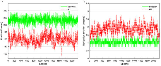
Figure 7.
Comparison of positioning accuracy and computation time between all satellite selection and the NSWOA. (a) Comparison of positioning accuracy for 2185 epochs. (b) Comparison of computation time for 2185 epochs.
From Figure 6 and Figure 7, it can be observed that the proposed NSWOA satellite selection algorithm strikes a balance between positioning accuracy and the number of selected satellites, resulting in a significant improvement in computational performance. With the positioning accuracy remaining constant at approximately , the number of selected satellites decreased from an average of about 22 to fewer than 6. In terms of computation time, this represents approximately 54.96% of the time required for selecting all visible satellites.
4. Discussion
The proposed NSWOA exhibits strong adaptability for dynamic satellite selection in dense LEO environments. With future constellations expected to exceed 10,000 satellites, scalability becomes critical. In our experiments involving over 6,000 satellites, the average number of visible satellites remained around 22 per epoch due to physical constraints like elevation angle and signal strength. NSWOA leverages these constraints to reduce the search space before optimization, ensuring computational efficiency. Even under growing satellite densities, the algorithm can maintain real-time performance by adjusting the population size and iteration count, while its convergence remains stable across all tested configurations.
For practical deployment, the proposed NSWOA is highly suitable for real-time implementation on embedded platforms such as UAVs. Although our experiments were conducted on a desktop CPU (i7-12700F), the algorithm achieved an average runtime of just 0.78 s per epoch, demonstrating both high computational efficiency and low solution latency. For embedded applications, the number of agents and iterations can be further reduced with minimal impact on optimization quality, as confirmed by convergence analysis.
To support real-time operation in resource-constrained environments, the algorithm’s modular design plays a crucial role. It features a fixed-size archive and constraint-based filtering, effectively limiting memory usage. Additionally, the computational structure of NSWOA allows for parallelization and hardware-level optimization on heterogeneous SoC platforms. Specifically,
- High-throughput tasks such as DGDOP computation and agent position updates can be offloaded to DSPs, GPUs, or FPGAs, supported by high-speed local memory;
- Control flow and decision logic are best handled by ARM Cortex-A/R cores;
- Data with frequent access patterns, such as the archive and position vectors, should be stored in on-chip SRAM or shared caches to reduce latency;
- SIMD/GPU thread-level parallelism is well suited for large-scale agent updates;
- To alleviate DDR memory pressure, intermediate results can be buffered using L2/L3 caches or tightly coupled memory (TCM).
These architectural advantages indicate that with modest adaptation, NSWOA can be effectively deployed for onboard satellite selection in real-time applications, particularly on large UAV platforms equipped with heterogeneous SoC architectures.
Future work will focus on real-time onboard experiments and flight testing to assess performance under real-world dynamics. Additionally, integrating 3D path estimation and inertial-assisted navigation is expected to improve robustness in high-maneuver scenarios. Deep Q-learning techniques, such as prioritized experience replay mechanisms, have also shown promise in enhancing control stability under time-varying signals [40]. Inspired by these methods, adaptive learning-based optimization strategies may be incorporated into the NSWOA framework to further advance intelligent navigation using non-cooperative LEO signals.
5. Conclusions
This study presents a fast satellite selection algorithm, NSWOA, for multi-constellation LEO satellite dynamic opportunistic navigation. Through both theoretical modeling and experiments, the key findings and contributions are summarized as follows:
The algorithm was evaluated over 2185 dynamic epochs using Doppler signals from multiple LEO constellations, including Starlink, Orbcomm, and Iridium. In terms of computational efficiency, it achieved average runtime reductions of 27.06% compared to GWO, 27.05% compared to PSO, and 68.57% compared to NSGA-II. Moreover, it consistently outperformed these benchmark algorithms in solution quality, demonstrating clear advantages in both speed and optimization performance.
NSWOA consistently exhibited rapid convergence and reliable performance across varying constraint scenarios. In fixed-number satellite selection, the algorithm required only 11 iterations on average to meet the navigation threshold, confirming its suitability for time-sensitive applications such as UAV-based positioning.
By introducing Pareto non-dominated sorting into the Whale Optimization Algorithm, the proposed NSWOA simultaneously minimizes both the DGDOP value and the number of selected satellites. It reduces the average number of selected satellites from 22 to fewer than 6 while maintaining a stable preset positioning accuracy of approximately 260 m. This enables a real-time balance between positioning accuracy and computational efficiency, reducing computation time to 54.96% compared to full satellite selection.
Author Contributions
Conceptualization, C.D.; methodology, C.D. and Y.C.; validation, C.D. and Y.C.; formal analysis, C.D. and B.Z.; investigation, Y.C.; resources, C.D. and B.Z.; writing—original draft preparation, C.D. and Y.C.; writing—review and editing, Y.C., C.D. and K.W.; visualization, Y.C.; supervision, C.D. and B.Z.; project administration, C.D., B.Z., L.L., L.Z. and M.W.; funding acquisition, C.D. All authors have read and agreed to the published version of the manuscript.
Funding
This research was funded by the National Natural Science Foundation of China (grant number 61973314) and the National Society Science Foundation of China (grant number 2024SKJJB037).
Institutional Review Board Statement
Not applicable.
Informed Consent Statement
Not applicable.
Data Availability Statement
The data that support the findings of this study are available from the corresponding authors upon reasonable request.
Conflicts of Interest
According to the policy as well as our moral obligation, we declare that there are no relevant conflicts of interest.
References
- Su, Y.; Liu, Y.; Zhou, Y.; Yuan, J.; Cao, H.; Shi, J. Broadband LEO satellite communications: Architectures and key technologies. IEEE Wirel. Commun. 2019, 26, 55–61. [Google Scholar] [CrossRef]
- Pritchard-Kelly, R.; Costa, J. Low earth orbit satellite systems: Comparisons with geostationary and other satellite systems, and their significant advantages. J. Telecommun. Digit. Econ. 2022, 10, 1–22. [Google Scholar] [CrossRef]
- Xiao, Z.; Yang, J.; Mao, T.; Xu, C.; Zhang, R.; Han, Z.; Xia, X.-G. LEO satellite access network (LEO-SAN) towards 6G: Challenges and approaches. IEEE Wirel. Commun. 2022, 31, 89–96. [Google Scholar] [CrossRef]
- Viterale, F.D.C. Transitioning to a New Space Age in the 21st Century: A Systemic-Level Approach. Systems 2023, 11, 232. [Google Scholar] [CrossRef]
- Prol, F.S.; Ferre, R.M.; Saleem, Z.; Valisuo, P.; Pinell, C.; Lohan, E.S.; Elsanhoury, M.; Elmusrati, M.; Islam, S.; Celikbilek, K.; et al. Position, Navigation, and Timing (PNT) through Low Earth Orbit (LEO) satellites: A survey on current status, challenges, and opportunities. IEEE Access 2022, 10, 83971–84002. [Google Scholar] [CrossRef]
- Reid, T.G.R.; Walter, T.; Enge, P.K.; Lawrence, D.; Cobb, H.S.; Gutt, G.; O'Conner, M.; Whelan, D. Navigation from Low Earth Orbit. In Position, Navigation, and Timing Technologies in the 21st Century: Integrated Satellite Navigation, Sensor Systems, and Civil Applications; IEEE: Piscataway, NJ, USA, 2021; pp. 1359–1379. [Google Scholar] [CrossRef]
- Benzerrouk, H. Iridium Next LEO satellites as an alternative PNT in GNSS denied environments. Inside GNSS 2019, 14, 56–64. [Google Scholar]
- Tan, Z.; Qin, H.; Cong, L.; Zhao, C. New method for positioning using IRIDIUM satellite signals of opportunity. IEEE Access 2019, 7, 83412–83423. [Google Scholar] [CrossRef]
- Guo, S.; Zhou, W.; Zhang, J.; Sun, F.; Yu, D. Integrated constellation design and deployment method for a regional augmented navigation satellite system using piggyback launches. Astrodynamics 2021, 5, 49–60. [Google Scholar] [CrossRef]
- Cinelli, M.; Ortore, E.; Laneve, G.; Circi, C. Geometrical approach for an optimal inter-satellite visibility. Astrodynamics 2021, 5, 237–248. [Google Scholar] [CrossRef]
- Ries, L.; Limon, M.C.; Grec, F.-C.; Anghileri, M.; Prieto-Cerdeira, R.; Abel, F. LEO-PNT for augmenting Europe’s space-based PNT capabilities. In Proceedings of the 2023 IEEE/ION Position, Location and Navigation Symposium (PLANS), Monterey, CA, USA, 24–27 April 2023; pp. 329–337. [Google Scholar]
- Kassas, Z.M.; Morales, J.J.; Khalife, J.J. New-age satellite-based navigation STAN: Simultaneous tracking and navigation with LEO satellite signals. Inside GNSS Mag. 2019, 14, 56–65. [Google Scholar]
- Wang, L.; Chen, R.; Xu, B.; Zhang, X.; Li, T.; Wu, C. The challenges of LEO based navigation augmentation system–lessons learned from Luojia-1A satellite. In Proceedings of the China Satellite Navigation Conference, Beijing, China, 22–25 May 2019; pp. 298–310. [Google Scholar]
- Kassas, Z.; Neinavaie, M.; Khalife, J.; Khairallah, N.; Kozhaya, S.; Haidar-Ahmad, J.; Shadram, Z. Enter LEO on the GNSS Stage: Navigation with Starlink Satellites. 2021. Available online: https://escholarship.org/content/qt9td3n8wd/qt9td3n8wd.pdf (accessed on 4 July 2025).
- Li, B.; Ge, H.; Ge, M.; Nie, L.; Shen, Y.; Schuh, H. LEO enhanced global navigation satellite system (LeGNSS) for real-time precise positioning services. Adv. Space Res. 2019, 63, 73–93. [Google Scholar] [CrossRef]
- Ge, H.; Li, B.; Nie, L.; Ge, M.; Schuh, H. LEO constellation optimization for LEO enhanced global navigation satellite system (LeGNSS). Adv. Space Res. 2020, 66, 520–532. [Google Scholar] [CrossRef]
- Tan, Z.; Qin, H.; Cong, L.; Zhao, C. Positioning using IRIDIUM satellite signals of opportunity in weak signal environment. Electronics 2019, 9, 37. [Google Scholar] [CrossRef]
- Leng, M.; Lei, L.; Razul, S.G.; See, C.M. Joint synchronization and localization using Iridium ring alert signal. In Proceedings of the 10th International Conference on Information, Communications and Signal Processing (ICICS), Singapore, 2–4 December 2015; pp. 1–5. [Google Scholar]
- Hayek, S.; Kassas, Z.M. Modeling and compensation of timing and spatial ephemeris errors of non-cooperative LEO satellites with application to PNT. IEEE Trans. Aerosp. Electron. Syst. 2024, 61, 5579–5593. [Google Scholar] [CrossRef]
- Khalife, J.; Neinavaie, M.; Kassas, Z.M. Navigation with differential carrier phase measurements from megaconstellation LEO satellites. In Proceedings of the IEEE/ION Position, Location and Navigation Symposium (PLANS), Portland, OR, USA, 20–23 April 2020; pp. 1393–1404. [Google Scholar]
- Sun, X.; Wang, Y.; Su, J.; Li, J.; Xu, M.; Bai, S. Relative orbit transfer using constant-vector thrust acceleration. Acta Astronaut. 2025, 229, 715–735. [Google Scholar] [CrossRef]
- Jardak, N.; Adam, R. Practical use of Starlink downlink tones for positioning. Sensors 2023, 23, 3234. [Google Scholar] [CrossRef]
- Grayver, E.; Nelson, R.; McDonald, E.; Sorensen, E.; Romano, S. Position and navigation using Starlink. In Proceedings of the 2024 IEEE Aerospace Conference, Big Sky, MT, USA, 2–9 March 2024; pp. 1–12. [Google Scholar]
- Neinavaie, M.; Shadram, Z.; Kozhaya, S.; Kassas, Z.M. First results of differential Doppler positioning with unknown Starlink satellite signals. In Proceedings of the 2022 IEEE Aerospace Conference (AERO), Big Sky, MT, USA, 5–12 March 2022; pp. 1–14. [Google Scholar]
- Neinavaie, M.; Kassas, Z.M. Unveiling Starlink LEO satellite OFDM-like signal structure enabling precise positioning. IEEE Trans. Aerosp. Electron. Syst. 2024, 60, 2486–2489. [Google Scholar] [CrossRef]
- Kozhaya, S.; Kanj, H.; Kassas, Z.M. Multi-constellation blind beacon estimation, Doppler tracking, and opportunistic positioning with OneWeb, Starlink, Iridium NEXT, and Orbcomm LEO satellites. In Proceedings of the IEEE/ION Position, Location and Navigation Symposium, Monterey, CA, USA, 24–27 April 2023; pp. 1184–1195. [Google Scholar]
- Huang, C.; Qin, H.; Zhao, C.; Liang, H. Phase-time method: Accurate Doppler measurement for Iridium NEXT signals. IEEE Trans. Aerosp. Electron. Syst. 2022, 58, 5954–5962. [Google Scholar] [CrossRef]
- Yang, C.; Zang, B.; Gu, B.; Zhang, L.; Dai, C.; Long, L.; Zhang, Z.; Ding, L.; Ji, H. Doppler positioning of dynamic targets with unknown LEO satellite signals. Electronics 2023, 12, 2392. [Google Scholar] [CrossRef]
- Zhao, C.; Qin, H.; Wu, N.; Wang, D. Analysis of baseline impact on differential Doppler positioning and performance improvement method for LEO opportunistic navigation. IEEE Trans. Instrum. Meas. 2023, 72, 8501110. [Google Scholar] [CrossRef]
- Stanescu, D.; Buzducea, A. An Overview of Satellite Link Budget Sensitivity Based on Digital Modulation Schemes in Multi-Orbit Satellite Networks. Appl. Sci. 2025, 15, 3473. [Google Scholar] [CrossRef]
- Di, H.; Dong, T.; Liu, Z.; Wei, S.; Zhang, Q.; Zhang, D. Dynamic Reporting Nodes Selection Method for Network Awareness Based on Active–Passive Integrated Network Telemetry in LEO Satellite Networks. Appl. Sci. 2025, 15, 5938. [Google Scholar] [CrossRef]
- Höyhtyä, M.; Anttonen, A.; Majanen, M.; Yastrebova-Castillo, A.; Varga, M.; Lodigiani, L.; Corici, M.; Zope, H. Multi-Layered Satellite Communications Systems for Ultra-High Availability and Resilience. Electronics 2024, 13, 1269. [Google Scholar] [CrossRef]
- Kassas, Z.M.; Kozhaya, S.; Kanj, H.; Saroufim, J.; Hayek, S.W.; Neinavaie, M. Navigation with multi-constellation LEO satellite signals of opportunity: Starlink, OneWeb, Orbcomm, and Iridium. In Proceedings of the 2023 IEEE/ION Position, Location and Navigation Symposium (PLANS), Monterey, CA, USA, 24–27 April 2023; pp. 338–343. [Google Scholar]
- Jardak, N.; Jault, Q. The potential of LEO satellite-based opportunistic navigation for high dynamic applications. Sensors 2022, 22, 2541–2565. [Google Scholar] [CrossRef]
- Coello, C.A.C. Evolutionary multi-objective optimization: Some current research trends and topics that remain to be explored. Front. Comput. Sci. China 2009, 3, 18–30. [Google Scholar] [CrossRef]
- Mirjalili, S.; Lewis, A. The Whale Optimization Algorithm. Adv. Eng. Softw. 2016, 95, 51–67. [Google Scholar] [CrossRef]
- Deb, K.; Pratap, A.; Agarwal, S.; Meyarivan, T. A fast and elitist multiobjective genetic algorithm: NSGA-II. IEEE Trans. Evol. Comput. 2002, 6, 182–197. [Google Scholar] [CrossRef]
- Kennedy, J.; Eberhart, R. Particle swarm optimization. In Proceedings of the International Conference on Neural Networks (ICNN’95), Perth, WA, Australia, 27 November–1 December 1995; pp. 1942–1948. [Google Scholar]
- Mirjalili, S.; Mirjalili, S.M.; Lewis, A. Grey wolf optimizer. Adv. Eng. Softw. 2014, 69, 46–61. [Google Scholar] [CrossRef]
- Ben Hazem, Z. Study of Q-learning and deep Q-network learning control for a rotary inverted pendulum system. Discov. Appl. Sci. 2024, 6, 49. [Google Scholar] [CrossRef]
Disclaimer/Publisher’s Note: The statements, opinions and data contained in all publications are solely those of the individual author(s) and contributor(s) and not of MDPI and/or the editor(s). MDPI and/or the editor(s) disclaim responsibility for any injury to people or property resulting from any ideas, methods, instructions or products referred to in the content. |
© 2025 by the authors. Licensee MDPI, Basel, Switzerland. This article is an open access article distributed under the terms and conditions of the Creative Commons Attribution (CC BY) license (https://creativecommons.org/licenses/by/4.0/).