Optimal Operating Patterns for the Energy Management of PEMFC-Based Micro-CHP Systems in European Single-Family Houses

Abstract

Commercial proton exchange membrane fuel cell (PEMFC)-based micro-combined heat and power (micro-CHP) systems are operated by rule-based energy management systems (EMSs). These EMSs are easy to implement but do not perform an explicit economic optimization. On the other hand, an optimal EMS can explicitly incorporate an economic optimization, but its implementation is more complex and may not be viable in practice. In a previous contribution, it was shown that current rule-based EMSs do not fully exploit the economic potential of micro-CHP systems due to their inability to adapt to changing scenarios. This study investigates the economic performance and behavior of an optimal EMS in 46 scenarios within the European framework. This EMS is designed using a model predictive control approach, and it is formulated as a mixed integer linear programming problem. The results reveal that there are only four basic optimal operating patterns, which vary depending on the scenario. This finding enables the design of an EMS that is computationally simpler than the optimal EMS but capable of emulating it and, therefore, is able to adapt effectively to changing scenarios. This new EMS would improve the cost-effectiveness of PEMFC-based micro-CHP systems, reducing their payback period and facilitating their mass market uptake.

1. Introduction

Proton exchange membrane fuel cell (PEMFC)-based micro-combined heat and power (micro-CHP) systems can help to create a greener energy future in Europe [1,2,3]. Several studies in the current scientific literature address CHP systems based on PEMFC technology. A recent and particularly interesting example is presented in [4], where a PEMFC-based CHP system is combined with heat pumps to enhance energy efficiency, specifically targeting industrial installations. In the field of residential applications, there is a genuine interest in making these systems a reality at both the political and industrial levels [5]. The idea is that they will replace the current condensing boilers in the coming years. Several commercial products are already available, but mass market uptake has not yet been achieved, mainly due to their high cost.

Work is being done on several fronts to achieve this goal. The PACE (Pathway to a Competitive European Fuel Cell micro-Cogeneration market) project is a good example [6]. One of these fronts is improving the energy efficiency of the systems. This would increase their cost-effectiveness and reduce their payback period, making them more attractive to the end user [7].

System efficiency in the laboratory (nominal efficiency) is different from the global energy efficiency of the system when it is operating in a specific application. The latter depends, among other factors, on how the system is operated, i.e., on its energy management system (EMS) [8,9,10]. Commercial micro-CHP appliances implement rule-based EMSs, which are simple and easy to program [11,12,13,14].

In a previous study published by the authors, Navarro et al. [15], it was shown that these EMSs do not exploit the full savings potential of micro-CHP systems and that there is a significant profit margin that could be gained through better EMS design. The reason for this is that micro-CHP systems work in changing scenarios and rule-based EMSs are not able to adapt to changing scenarios. A scenario is the real-life situation in which the micro-CHP system is functioning. This situation is determined by several parameters that affect its economic performance, such as natural gas and electricity prices, household energy demands, etc. Therefore, the key to gaining this profit margin is that the EMS be able to adapt to changing scenarios. This means that it is possible to make micro-CHP systems more cost-effective simply by changing the way in which they are operated. This increase in cost-effectiveness can reach up to 14.5 percentage points in the annual energy bill.

An EMS capable of adapting and, therefore, theoretically able to exploit this profit margin is an optimal EMS, that is, a model predictive control (MPC)-based EMS. This solution is the most widely used in microgrids [16]. Unfortunately, and despite the above, an MPC-based EMS is complex, its computational cost is high, and it is sensitive to uncertainty in both the energy demands predictions and the model. These disadvantages make its practical implementation complex and uncertain.

However, the following question remains: What does the optimal EMS do? How does it adapt its behavior to the scenario? What does it do in each scenario? If this were known, it might be possible to design an EMS that emulates the optimal EMS. This new EMS would provide savings as high as the optimal EMS and would be as simple and fast as the rule-based EMSs, a solution, therefore, viable in practice. This prospect motivates the present research.

This contribution has four parts:

• An optimal EMS is designed.
• The parameters of the optimal EMS are adjusted (determination of the prediction horizon).
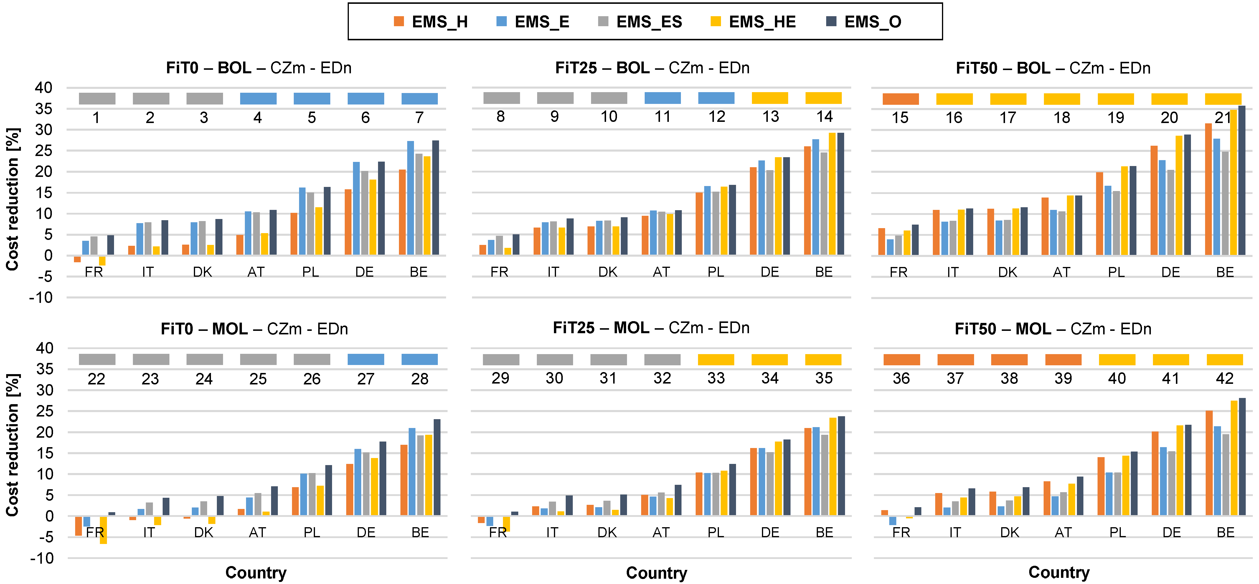
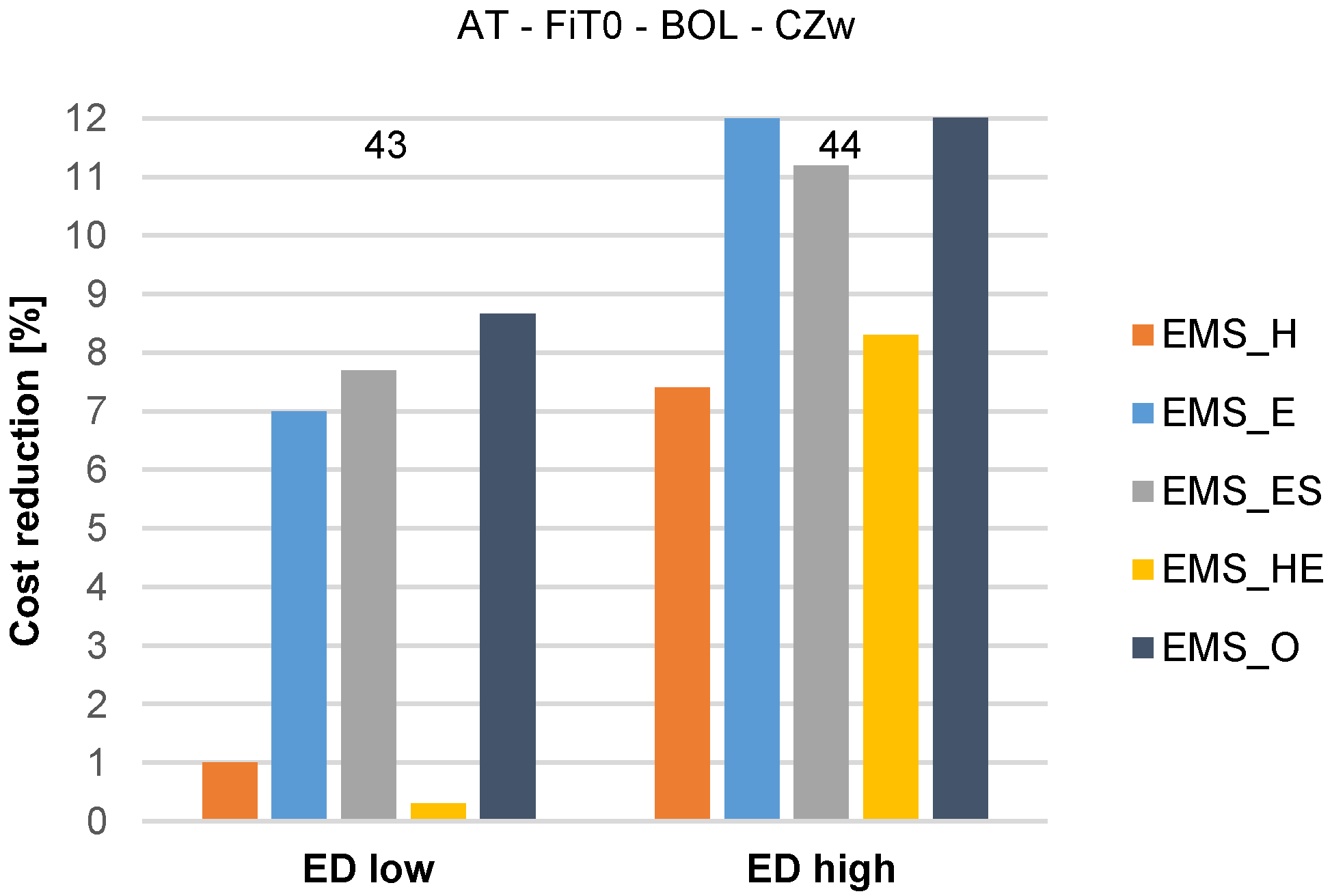
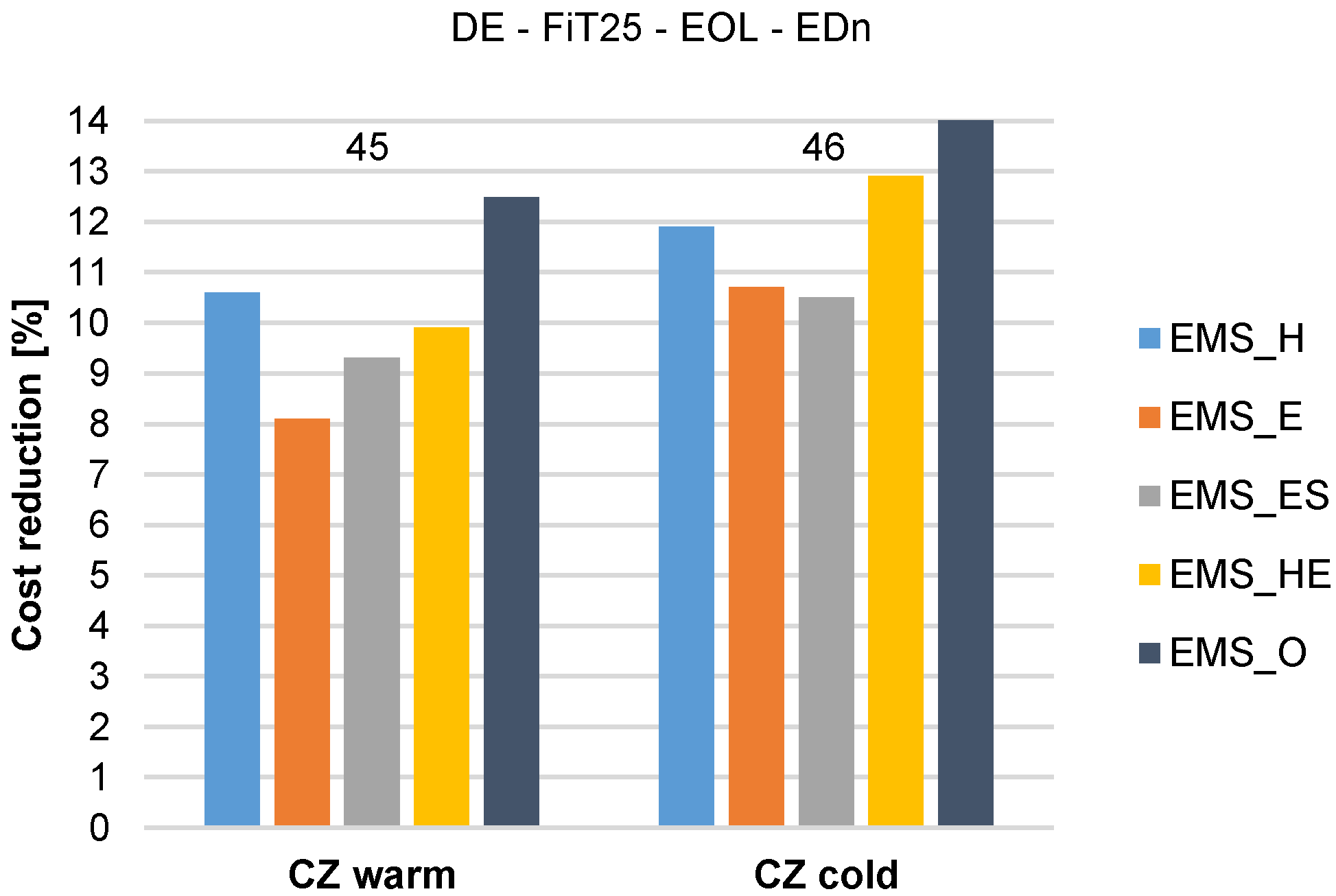
• The economic performance of the optimal EMS is evaluated in 46 scenarios belonging to the European framework, and it is compared with those achieved by four typical rule-based EMSs.
• The behavior of the optimal EMS is investigated in order to identify optimal operating patterns.

Regarding the first part, the optimal EMS designed is an MPC-based EMS that implements the formulation of a mixed integer linear programming (MILP) problem. It has been programmed in Matlab/Simulink. For the formulation of the MILP, the techno-economic model developed by the authors in Navarro et al. [15] has been used. This model represents an advance over the models available in the literature. The reason for this is that it is more precise and realistic, because it includes physical phenomena that are known to be essential for the correct evaluation of the economic performance and that other models have not taken into account: fuel cell degradation, auxiliary energy losses, heat losses in the thermal energy storage (TES), etc.

Regarding the second part, there is no previous work in the literature that has examined what the appropriate prediction horizon is for the optimal operation of micro-CHP systems.

Regarding the third part, there are several studies that have evaluated the economic performance of an optimal EMS for micro-CHP, with different purposes [17,18,19,20,21,22,23,24,25]. One of these purposes is to determine how much economic benefit the optimal EMS achieves compared to rule-based EMSs. In effect, it is precisely against rule-based EMSs that the optimal EMS must be evaluated and compared, since these are the EMSs currently in use and the ones the optimal EMS would replace if it surpassed them in economic performance. In this respect, the main deficiency of these works is that none of them include in their comparison the four rule-based EMSs that the authors showed to be relevant, namely (1) heat-led, (2) electricity-led, (3) heat-and-electricity-led, and (4) electricity-led switch off in summer (see Navarro et al. [15]). Because of this, there is still no well-established result on how much profit an optimal EMS achieves compared to rule-based EMSs.

Finally, regarding the fourth part, only one study, Hawkes et al. [17], has investigated the behavior of an optimal EMS for micro-CHP systems and identified optimal operating patterns. This fourth task, however, remains of interest and needs to be addressed again, despite having been carried out by a previous work, for three reasons.

First, in Hawkes et al. [17], the micro-CHP system was based on an SOFC (solid oxide fuel cell), not a PEMFC. There are enough differences between these two technologies to suggest that the optimal EMS behavior might be different in each case. The study by Ozawa and Kudoh [25] provides additional evidence in support of this hypothesis.

Second, the study by Hawkes et al. [17] was limited to the United Kingdom, so its energy prices space is considerably smaller than the one in Europe. A larger energy prices space could reveal new optimal behaviors not detected by Hawkes. The results of Navarro et al. [15] represent strong evidence in favor of this hypothesis. In effect, they showed that a change in the energy prices causes the best rule-based EMS to change.

Third, Hawkes et al. [17] say nothing about how stack degradation influences the behavior of the optimal EMS. Stack degradation is a fundamental phenomenon that greatly affects the performance of the micro-CHP system throughout its lifetime; see Navarro et al. [15] (Section 2.1). Furthermore, Navarro et al. [15] showed that changes in the stack degradation level also cause the best rule-based EMS to change. This fact suggests that the behavior of the optimal EMS is very likely to change with the stack degradation level.

In summary, regarding the optimal EMS behavior (fourth part or task), the knowledge gap is large. In effect, the following are not known:

• Whether or not the results of Hawkes et al. [17] will be the same for a PEMFC-based system.
• If their conclusions remain valid for a wider energy price range, which is what exists in Europe.
• What effect stack degradation has on the optimal EMS behavior.

Table 1. Comparison of this study with previous research.

	Hawkes et al. [17] a	Hawkes et al. [19]	Houwing et al. [18]	Ren et al. [21] b	Shaneb et al. [20]	This study
Micro-CHP system technology	SOFC	PEMFC	PEMFC	PEMFC	PEMFC	PEMFC
	Gas engine			Gas engine
	Stirling engine
Stack degradation	✗	✓	✗	✗	✗	✓
Auxiliary energy losses	✓	✓	✗	✓	✗	✓
Heat losses in the TES	✗	✗	✗	✓	✗	✓
Part-load electrical efficiency	✓	✓	✗	✓	✗	✓
TES charge and discharge efficiencies	✓	✓	✗	✗	✓	✓
Micro-CHP ramp constraints	✗	✓	✓	✗	✓	✓
Startup and shutdown times	✗	✓	✓	✗	✗	✓
Startup and shutdown costs	✗	✓	✓	✗	✗	✓
Heat dumping cost	✗	✗	${\mathbf{✗} }^c$	✗	${\mathbf{✗} }^d$	✓
Optimization problem formulation	NLP e	MILP	MILP	MILP	${\mathrm{LP} }^f$	MILP
Optimization horizon	1 day	1 day	1 day	1 day	1 day	8 h
Demand profiles resolution	5 min	5 min	15 min	1 h	1 h	1 min
Time period studied	Annual	Annual/lifetime	Annual	Annual	Annual	Annual
Demand profiles representativeness	Indicative of UK average residential demand	One large UK dwelling in north London	Indicative of NL average residential demand	One single-family house in Kitakyushu, Japan	One dwelling in North West of London	Reference load profiles according to VDI Guide- line 4655
Simulation approach	Unk.	Sample day profiles	Complete annual profiles	Unk.	Complete annual profiles	Complete annual profiles
Number of parameters studied	2	5	1	1	4	5
Parameters whose influence is studied	Energy prices	Start/stop costs	Electricity tariff structures	Micro-CHP technology	FiT	Energy prices
	FiT	Ramp limits			Government incentives	FiT
		Maximum turndown			Carbon tax	Stack degradation
		Minimum up-time			PEMFC nominal power	Climate zone
		Stack degradation				HPR demand side
Number of scenarios evaluated	15	6	3	2	60	46
Number of EMSs compared	3	1	2	2	3	5
EMSs compared	Heat-led	Optimal strategy	Heat-led	Minimum CO2 operation	Heat-led	Heat-led
	Electricity-led		Optimal strategy	Optimal strategy	Electricity-led	Electricity-led
	Optimal strategy				Optimal strategy	Heat-and-electricity-led
						Electricity-led switch off in summer
						Optimal strategy

^a The description of the model and the formulation of the optimization problem are in [26]. ^b The model used is presented in [27]. ^c The authors assume that heat cannot be dumped. ^d The authors assume that heat dumping is not allowed. ^e Non-linear programming. ^f The formulation is LP (linear programming) because there are no startups/shutdowns and because there is no piecewise electrical dispatch. ✗: Physical phenomenon not taken into account. ✓: Physical phenomenon taken into account.

compares this study with five previous studies. The compared features are grouped into six blocks: (1) micro-CHP system technology, (2) modeled physical phenomena, (3) optimization problem formulation, (4) energy demand profiles, (5) parameters included in the analysis, and (6) compared operating strategies.

2. Methods

This section begins with a description of the micro-CHP system, the household, the energy demand profiles, the four rule-based EMSs against which the optimal EMS is compared, the scenario characterization, and the economic performance index. This description is brief since its content is addressed in detail in Navarro et al. [15].

The micro-CHP system is shown in Figure 1. Its main characteristics are listed in

Table 2. Characteristics of the micro-CHP system [15].

Characteristic	Value
Nominal electrical power (BOL)	0.75 kW
Minimum electrical power	0.25 kW
Nominal thermal power (BOL)	1.07 kW
Electrical efficiency (BOL)	31.3% (HHV)
Thermal efficiency (BOL)	44.7% (HHV)
Maximum ramp	0.2 kW/min
Startup time	45 min
Natural gas consumption at startup	1.5 kW
Power consumption at startup	75 W
Shutdown time	5 min
Power consumption during shutdown	50 W
Auxiliary boiler nominal thermal power	26.5 kW
Auxiliary boiler efficiency	93%
Tank volume	200 L
Tank temperature range	50–70 °C
Tank capacity	4.572 kWh

. A techno-economic model of that system was developed and presented in Navarro et al. [15], Section 2.2. The simulations in the current paper were performed with that model. Although the model does not incorporate low-level phenomena such as air and hydrogen pressures and flow rates, or fuel cell humidity, it does include all the physical phenomena considered relevant in the literature on PEMFC-based micro-CHP systems, such as fuel cell degradation, auxiliary energy losses, heat losses in the TES, and varying electrical efficiency as a function of operating point, among others. The complete list is shown in Table 1, second block. Among the modeled phenomena, the four mentioned are of particular importance. If these four phenomena are not taken into account, the validity of the results is uncertain. For a discussion of the importance of incorporating these four phenomena into the model, see Navarro et al. [15], Section 2.1.

The characteristics of the house served by the micro-CHP system are shown in

Table 3. Characteristics of the house [15].

Characteristic	Value
Type of building	Single-family house
Location	Oberhausen, Germany
N° of occupants	3
Annual heating demand	11,000 kWh
Annual electricity demand	5250 kWh
Annual DHW demand	1500 kWh

. The annual energy demand profiles of the house used in the simulations are of three types: (1) heat demand for heating, (2) heat demand for DHW (domestic hot water), and (3) electricity demand. The profiles were generated according to the VDI Guideline 4655 [28] standard. They are annual profiles and have a temporal resolution of one minute. For a detailed description, see Navarro et al. [15], Sections 3.2, 5.2, and 5.3. These profiles satisfy three requirements highlighted in the literature, namely, (1) they have a sufficiently high temporal resolution, (2) they are annual profiles, and (3) they are representative of the existing diversity in the case study (Europe). For a discussion of the importance of using profiles that satisfy these three requirements, see Navarro et al. [15], Section 3.1. The assumptions and the limitations of the energy demand profiles (heating, DHW, and electricity) used in the simulations are described in the VDI Guideline 4655 [28] and in Navarro et al. [15]. The characteristics of the demand profiles used in this study are compared with those of profiles used in other works in Table 1, fourth block.

The simulation approach, in Table 1, fourth block, describes the way in which the simulations are performed. Sample day profiles means that a few days, representative of each season, are simulated and the annual results are calculated from the results obtained with those days, given an estimate of the number of days of each type. Complete annual profiles means that the simulations performed are annual. Methodologically, it is not the same to simulate with a few typical days and then estimate the annual economic savings as it is to simulate with annual demand profiles. No one has yet demonstrated that the former procedure provides the same results as the latter. For that reason, and because the second procedure is more realistic, it was preferred. Using demand profiles with a resolution of 1 min and simulating full years implied a high computational load. The 46 simulations took about 6 months, using 7 desktop computers.

The four rule-based EMSs with respect to which the optimal EMS is compared are (1) heat-led strategy (EMS_H), (2) electricity-led strategy (EMS_E), (3) electricity-led-switch-off-in-summer strategy (EMS_ES), and (4) heat-and-electricity-led strategy (EMS_HE). For a detailed description, see Navarro et al. [15], Section 4. In the same study, it was shown that the four EMSs considered are relevant, because each of them proved to be the best in a considerable number of scenarios. For this reason, it is important that the optimal EMS be compared with all four, otherwise the picture would be incomplete and the question of how much economic benefit an optimal EMS provides compared to rule-based EMSs could not be answered definitively.

The comparison of the optimal EMS with the rule-based EMSs was performed in 46 different scenarios. A scenario is defined by five parameters: (1) spark gap, (2) FiT (feed-in tariff), (3) D (degradation), (4) CZ (climate zone), and (5) HPR (demand side heat to power ratio). The spark gap is the ratio between the price of electricity and the price of natural gas. In Navarro et al. [15], it was shown that the percentage savings that the micro-CHP system achieves with respect to the reference system depends on the spark gap, not on prices. For this reason, the spark gap is used in the characterization of the scenario, instead of prices.

The electricity and natural gas prices corresponding to the spark gap values used are those of seven European Union countries during the first half of 2021, namely, France (FR), Italy (IT), Denmark (DK), Austria (AT), Poland (PL), Germany (DE), and Belgium (BE). FiT is the price of the electricity fed into the grid, as a percentage of the electricity price. This parameter can take three values: 0%, 25%, and 50%. D is the stack degradation level. It takes three values: 0% (BOL), 10% (MOL), and 20% (EOL).

CZ is the climate of the location of the house. It can take three values: warm (CZw), mild (CZm), and cold (CZc). The climate zone (CZ) determines the annual heating demand and the annual sequence of days. This is described in Navarro et al. [15], Sections 5.2 and 5.3. The annual demands corresponding to each CZ are 10,426 kWh (CZw), 13,752 kWh (CZm), and 16,917 kWh (CZc). A representation of the annual sequences of days corresponding to each CZ can be found in Navarro et al. [15], Figure 8. The annual heat demand for DHW and the annual electricity demand are 1500 kWh and 5250 kWh, respectively, the same for the three CZs.

HPR is the ratio between the annual heat demand and the annual electricity demand. It can take three values: ED low (EDl), ED nominal (EDn), and ED high (EDh). EDn is 5250 kWh. EDl and EDh represent excursions of +20% and −20%, with respect to EDn. The values of the HPRs associated with each ED can be found in Navarro et al. [15], Table 6.

For a justification of the five parameters chosen for the characterization of the scenario, as well as the values that each of them can take, see Navarro et al. [15], Section 5.1.

In each of the 46 scenarios, the supply of the energy demand of the house, with the micro-CHP system operated by the optimal EMS, was simulated for one year. For the comparison of the EMSs performances, the annual cost reduction achieved with the micro-CHP system with respect to the reference system (a condensing boiler and a connection to the electrical grid, i.e., traditional supply) was used as an index, Equation (1). For a rationale for the chosen index and for additional details on its terms, see Navarro et al. [15], Section 5, first three paragraphs. The results obtained with the four rule-based EMSs in the 46 scenarios are from Navarro et al. [15].

$$CR=100{\displaystyle \frac{C_{RS}-C_{\mu CHP}}{C_{RS}}}$$

(1)

2.1. Design of the Optimal EMS

This section presents the design of the optimal EMS (first part of this contribution).

The optimal EMS is an MPC controller. At each sampling time k, the optimal EMS performs the following steps:

• Acquires process state information (demands, TES state of charge (SOC), prices, etc.).
• Acquires a prediction of the energy demand profiles for a given time horizon.
• Calculates the sequence of control action values that minimize the operating cost of the micro-CHP system within the prediction horizon.
• Applies the values of instant k and returns to step 1.

For the calculation in step 3, the optimal EMS solves a MILP type optimization problem. The objective function (operating cost) is evaluated within a given time window, namely, from the current instant k to the future instant $k+HP$. The constant $HP$ is the prediction horizon. The predictions of energy demands are assumed to be perfect. This is the best case for the optimal EMS.

Next, the MILP optimization problem is formulated. This formulation follows closely the one developed by Hawkes et al. [19] and later also used by Palop [29]. The optimization problem consists of minimizing the objective function ${\mathbf{f}}^{\mathrm{T}}\mathbf{x}$, Equation (2), subject to the constraints defined in Equations (3)–(5).

$$\underset{\mathbf{x}}{min}{\mathbf{f}}^{\mathrm{T}}\mathbf{x}$$

(2)

$$\mathbf{A}\mathbf{x}\le \mathbf{b}$$

(3)

$${\mathbf{A}}_{\mathbf{eq}}\mathbf{x}={\mathbf{b}}_{\mathbf{eq}}$$

(4)

$$\mathbf{lb}\le \mathbf{x}\le \mathbf{ub}$$

(5)

The vector $\mathbf{x}$ in (2) is the vector of decision variables. There is a distinction between decision variables and control actions. For a given instant k, there are 16 decision variables (Nomenclature section) but only 4 control actions: $P{e}_{SYSre{f}_k}$, $Pt{h}_{ABre{f}_k}$, $Pt{h}_{Dre{f}_k}$, and $ON/OF{F}_k$ (Figure 1). $P{e}_{SYSre{f}_k}$ is the sum of the piecewise electrical outputs, Equation (6), and $ON/OF{F}_k=Y_{T{0}_k}$.

$$P{e}_{SYSre{f}_k}=P{e}_{T{0}_k}+P{e}_{T{1}_k}+P{e}_{T{2}_k}+P{e}_{T{3}_k}+P{e}_{T{4}_k}$$

(6)

The objective function ${\mathbf{f}}^{\mathrm{T}}\mathbf{x}$ is the operating cost of the micro-CHP system, Equation (7), whose coefficients are given by Equations (8)–(12).

$$\begin{array}{c}\hfill F\left(\mathbf{x}\right)=\sum _{i=0}^{HP-1}(\sum _{n=0}^4{c}_{P{e}_{Tn}}P{e}_{T{n}_{k+i}}+c_{Pt{h}_{AB}}Pt{h}_{ABre{f}_{k+i}}+c_{Pt{h}_D}Pt{h}_{Dre{f}_{k+i}}+\\ \hfill +c_{P{e}_{buy}}P{e}_{bu{y}_{k+i}}+c_{P{e}_{sell}}P{e}_{sel{l}_{k+i}}+S_{s{t}_{k+i}}+S_{of{f}_{k+i}})\end{array}$$

(7)

$$c_{P{e}_{Tn}}={\displaystyle \frac{T_{s}P{r}_{ng}{K}_{n{g}_n}}{60r{e}_{SY{S}_N}(1-D)}}\forall n\in \{0,\dots ,4\}$$

(8)

$$c_{Pt{h}_{AB}}={\displaystyle \frac{T_{s}P{r}_{ng}}{60rt{h}_{AB}}}$$

(9)

$$c_{Pt{h}_D}={\displaystyle \frac{T_{s}P{r}_{el}{K}_{cool}}{60}}$$

(10)

$$c_{P{e}_{buy}}={\displaystyle \frac{T_{s}P{r}_{el}}{60}}$$

(11)

$$c_{P{e}_{sell}}=-{\displaystyle \frac{T_{s}P{r}_{FiT}}{60}}$$

(12)

The following describes the constraint Equations (3)–(5) that the solutions of Equation (2) must satisfy.

The SOC of the TES must be kept within minimum and maximum limits:

$$SO{C}_{min}\le SO{C}_{k+i}\le SO{C}_{max}\forall i\in \{1,\dots ,HP\}$$

(13)

The micro-CHP system model includes equations that model the electrical and thermal performances of the system, see Navarro et al. [15], Equations (1) and (2), and Figure 2. These equations are nonlinear. In order to apply the MILP methodology, the model must be linear. It is therefore necessary, as a preliminary step, to linearize these equations. The piecewise linearization of the electrical performance curve is described in Appendix A. This piecewise linearization entails nine additional constraints, Equations (14)–(18). These constraints force the dispatch order to be T0, T1, …, T4 [19]. The micro-CHP system startup time ($t_d$) is incorporated into the formulation as in [29].

$$P{e}_{T{0}_{k+i}}\le P{e}_1{Y}_{T{0}_{k+i-t_d}}\forall i\in \{0,\dots ,HP-1\}$$

(14)

$$P{e}_1{Y}_{T{0}_{k+i-t_d}}\le P{e}_{T{0}_{k+i}}\forall i\in \{0,\dots ,HP-1\}$$

(15)

$$P{e}_{T{1}_{k+i}}\le (P{e}_2-P{e}_1)Y_{T{0}_{k+i-t_d}}\forall i\in \{0,\dots ,HP-1\}$$

(16)

$$P{e}_{T{(n+1)}_{k+i}}\le (P{e}_{n+2}-P{e}_{n+1})Y_{T{n}_{k+i}}\forall n\in \{1,\dots ,3\},\forall i\in \{0,\dots ,HP-1\}$$

(17)

$$(P{e}_{n+1}-P{e}_n)Y_{T{n}_{k+i}}\le P{e}_{T{n}_{k+i}}\forall n\in \{1,\dots ,3\},\forall i\in \{0,\dots ,HP-1\}$$

(18)

The constraints formulated in Equations (19) and (20) prevent the simultaneous purchase and sale of electricity.

$$P{e}_{bu{y}_{k+i}}\le P{e}_{bu{y}_{max}}(1-Y_{re{d}_{k+i}})\forall i\in \{0,\dots ,HP-1\}$$

(19)

$$P{e}_{sel{l}_{k+i}}\le P{e}_{sel{l}_{max}}{Y}_{re{d}_{k+i}}\forall i\in \{0,\dots ,HP-1\}$$

(20)

Starting the micro-CHP system has a fixed cost that is not included in the electrical performance curve. In the model, it is assumed that, during startup, the system consumes electricity and natural gas, producing neither electricity nor heat. The cost of a startup is $s_{start}$. The startup cost is incorporated into the optimization problem via the constraint in Equation (21). When there is a change in $Y_{T0}$ from 0 to 1 (a startup), the constraint Equation (21) forces $S_{st}=s_{start}$, which penalizes $F\left(\mathbf{x}\right)$, Equation (7), charging the objective function with the startup cost.

$$s_{start}(Y_{T{0}_{k+i}}-Y_{T{0}_{k+i-1}})\le S_{s{t}_{k+i}}\forall i\in \{0,\dots ,HP-1\}$$

(21)

There is also a shutdown time, during which the micro-CHP system consumes electricity, producing neither electricity nor heat. The cost of a shutdown is $s_{of{f}_e}$. Analogously to the startup, the shutdown cost is incorporated into the optimization problem by the following constraint, Equation (22):

$$s_{of{f}_e}(Y_{T{0}_{k+i-1}}-Y_{T{0}_{k+i}})\le S_{of{f}_{k+i}}\forall i\in \{0,\dots ,HP-1\}$$

(22)

There is a limit on the rate at which the stack can ramp from one operating point to another (0.2 kW/min). This limit is incorporated into the optimization problem through the constraints in Equations (23) and (24), up and down cases, respectively. These constraints do not apply during the startup. Otherwise, startup would be impossible, since the minimum operating power of the micro-CHP system is 0.25 kW.

$$P{e}_{SY{S}_{re{f}_{k+i}}}-P{e}_{SY{S}_{re{f}_{k+i-1}}}\le ram{p}_{up}\forall i\in \{0,\dots ,HP-1\}$$

(23)

$$-P{e}_{SY{S}_{re{f}_{k+i}}}+P{e}_{SY{S}_{re{f}_{k+i-1}}}\le ram{p}_{down}\forall i\in \{0,\dots ,HP-1\}$$

(24)

The sum of the electric power flows must equal zero, Equation (25). This is the only equality-type constraint in the optimization problem.

$$P{e}_{SY{S}_{k+i}}+P{e}_{bu{y}_{k+i}}-P{e}_{sel{l}_{k+i}}-P{e}_{de{m}_{k+i}}=0\forall i\in \{0,\dots ,HP-1\}$$

(25)

Finally, the values that the decision variables can take are limited. These limits constitute constraints in the optimization problem, Equations (26)–(34).

$$0\le P{e}_{T{n}_{k+i}}\le (P{e}_{n+1}-P{e}_n)\forall n\in \{0,\dots ,4\},\forall i\in \{0,\dots ,HP-1\}$$

(26)

$$0\le Y_{T{n}_{k+i}}\le 1\forall n\in \{0,\dots ,3\},\forall i\in \{0,\dots ,HP-1\}$$

(27)

$$Pt{h}_{A{B}_{min}}\le Pt{h}_{A{B}_{re{f}_{k+i}}}\le Pt{h}_{A{B}_{max}}\forall i\in \{0,\dots ,HP-1\}$$

(28)

$$Pt{h}_{D_{min}}\le Pt{h}_{D_{re{f}_{k+i}}}\le Pt{h}_{D_{max}}\forall i\in \{0,\dots ,HP-1\}$$

(29)

$$0\le P{e}_{bu{y}_{k+i}}\le P{e}_{bu{y}_{max}}\forall i\in \{0,\dots ,HP-1\}$$

(30)

$$0\le P{e}_{sel{l}_{k+i}}\le P{e}_{sel{l}_{max}}\forall i\in \{0,\dots ,HP-1\}$$

(31)

$$0\le Y_{re{d}_{k+i}}\le 1\forall i\in \{0,\dots ,HP-1\}$$

(32)

$$0\le S_{s{t}_{k+i}}\le s_{start}\forall i\in \{0,\dots ,HP-1\}$$

(33)

$$0\le S_{of{f}_{k+i}}\le s_{of{f}_e}\forall i\in \{0,\dots ,HP-1\}$$

(34)

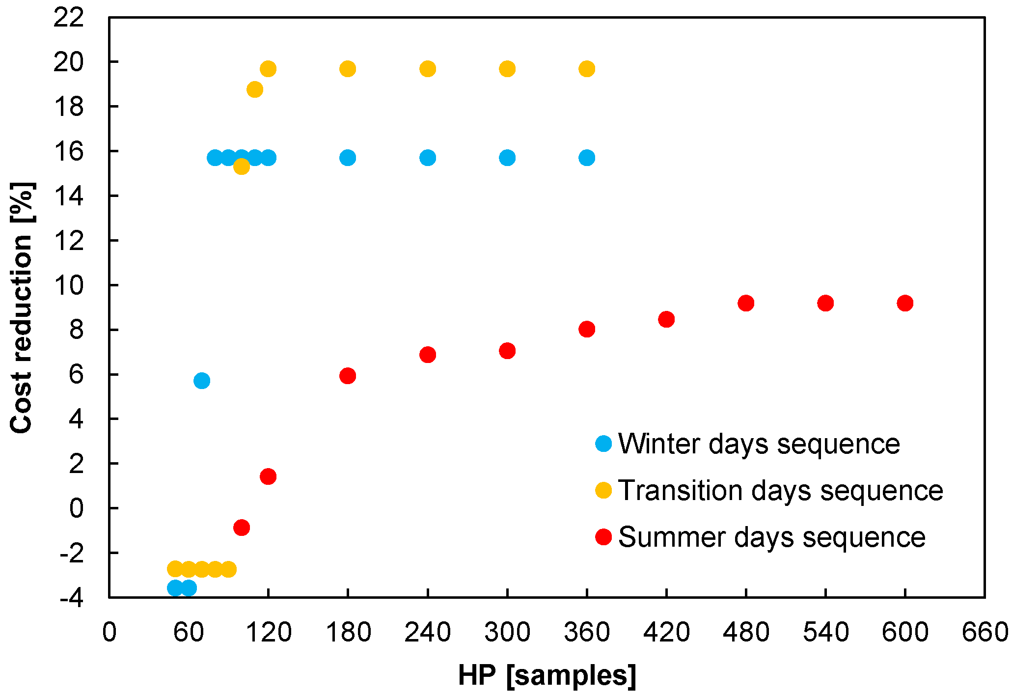
2.2. Determination of the Prediction Horizon

This section describes the methodology used to determine the prediction horizon (second part of this contribution).

Choosing the right HP for the optimal EMS is not trivial. For micro-CHP systems there is no analytical method to determine the HP. In general, the HP value depends on the dynamics of the process. For micro-CHP systems, therefore, the HP will depend mainly on the volume of TES and the profile of thermal energy demand, which are the two factors that determine the filling and emptying times of the TES.

Choosing the right HP is crucial. An HP that is too long unnecessarily increases the computation time and may make the implementation of the optimal EMS impractical. On the other hand, if the HP is too short, the optimal EMS will not find the best strategy (from an economic point of view). Despite its importance, in the literature on micro-CHP systems the determination of the correct prediction horizon has received hardly any attention. Among the papers included in the literature review presented in the Introduction (Section 1), only in Houwing et al. [18] is a brief justification of the chosen HP provided.

To determine the HP, a preliminary study was carried out, i.e., prior to the running of the 46 simulations. The starting hypothesis in this study was that the higher the HP, the greater the savings, up to a certain value beyond which the savings no longer increase. The plausibility of this hypothesis is justified by the fact that seeing the possible behavior of the system in a longer future time offers more degrees of freedom to operate.

A total of 161 simulations were conducted. In each of them, the demand supply was simulated over a sequence of days, with the micro-CHP system operated by the optimal EMS. These sequences varied in length (3, 4, or 5 days) and in type of day (winter, summer, transition, or a mix of these three). All simulations were performed under the same scenario (spark gap PL, FiT0, BOL, CZw, EDn) with SOC = 50% and the micro-CHP system initially turned off. Each simulation was repeated several times, increasing the HP until the savings stabilized.

Figure 2 presents a representative sample of the results. In winter, the heat demand is high, the TES empties quickly, and the HP can be small. In summer, the heat demand is low (only for DHW), the TES empties slowly, and the HP needs to be large. Based on the results of this preliminary study, HP = 80 was chosen for winter days, HP = 120 for transition days, and HP = 480 for summer days. Subsequently, during the running phase of the 46 simulations, in some of them, these HP values had to be increased to achieve stabilized savings. In some cases, this increase in HP reached 360 samples for winter days and 420 for transition days. Below, Section 4 will discuss the results regarding the prediction horizon in more detail.

3. Results

The presentation of the results is divided into two subsections: Section 3.1 shows the economic performance of the optimal EMS (third part of this contribution) and Section 3.2 reveals its behavior (fourth part of this contribution).

3.1. Evaluation of the Economic Performance of the Optimal EMS

Figure 3 shows the results of 42 out of the 46 simulated scenarios, presented in a 2 × 3 matrix. In the figure, the scenarios differ in three parameters: spark gap (country), FiT (column), and degradation level (row). The numerical results, as well as the parameter values for each scenario, are listed in

Table 4. Economic performance of the optimal EMS compared to those achieved by the rule-based EMSs. The numbers for the rule-based EMSs come from Navarro et al. [15]. The bold numbers indicate the best rule-based EMS.

Sce.	Ctry.	${\mathbf{Pr}}_{\mathbf{el}}$	${\mathbf{Pr}}_{\mathbf{ng}}$	Spark Gap	FiT	D	CZ	HPR	EMS_H	EMS_E	EMS_ES	EMS_HE	EMS_O	$\mathbf{\Delta }$	$\mathbf{\Phi }$	$\mathbf{\Psi }$
		[ct/kWh]	[ct/kWh]	[-]	[%]	[-]	[-]	[-]	[%]	[%]	[%]	[%]	[%]	[pp]	[%]	[%]
1	FR	19.33	6.78	2.85	0	BOL	CZm	EDn	−1.5	3.5	4.5	−2.3	4.9	0.4	5.1	0.3
2	IT	22.59	7.03	3.21	0	BOL	CZm	EDn	2.3	7.7	7.9	2.2	8.4	0.5	5.6	0.3
3	DK	29.00	8.95	3.24	0	BOL	CZm	EDn	2.6	7.9	8.2	2.5	8.7	0.5	5.2	0.3
4	AT	22.16	6.36	3.48	0	BOL	CZm	EDn	4.9	10.5	10.3	5.3	10.9	0.4	8.3	0.3
5	PL	15.48	3.76	4.12	0	BOL	CZm	EDn	10.2	16.2	15.0	11.5	16.3	0.1	5.5	0.3
6	DE	31.93	6.47	4.94	0	BOL	CZm	EDn	15.8	22.3	20.1	18.1	22.4	0.1	0.7	0.4
7	BE	27.02	4.68	5.77	0	BOL	CZm	EDn	20.5	27.3	24.3	23.6	27.5	0.2	0.7	0.3
8	FR	19.33	6.78	2.85	25	BOL	CZm	EDn	2.5	3.7	4.6	1.8	5.0	0.4	8.8	3.4
9	IT	22.59	7.03	3.21	25	BOL	CZm	EDn	6.6	7.9	8.1	6.6	8.8	0.7	8.6	3.8
10	DK	29.00	8.95	3.24	25	BOL	CZm	EDn	6.9	8.2	8.3	6.9	9.1	0.8	8.6	3.8
11	AT	22.16	6.36	3.48	25	BOL	CZm	EDn	9.4	10.7	10.4	9.8	10.7	0.0	13.5	3.5
12	PL	15.48	3.76	4.12	25	BOL	CZm	EDn	15.0	16.5	15.2	16.4	16.8	0.3	8.8	3.7
13	DE	31.93	6.47	4.94	25	BOL	CZm	EDn	21.0	22.6	20.3	23.4	23.4	0.0	1.9	0.5
14	BE	27.02	4.68	5.77	25	BOL	CZm	EDn	26.0	27.6	24.5	29.2	29.2	0.0	1.8	0.5
15	FR	19.33	6.78	2.85	50	BOL	CZm	EDn	6.6	3.9	4.8	6.0	7.4	0.8	6.4	0.4
16	IT	22.59	7.03	3.21	50	BOL	CZm	EDn	10.9	8.1	8.3	11.0	11.3	0.3	12.6	0.6
17	DK	29.00	8.95	3.24	50	BOL	CZm	EDn	11.2	8.4	8.5	11.3	11.6	0.3	12.6	0.5
18	AT	22.16	6.36	3.48	50	BOL	CZm	EDn	13.9	10.9	10.6	14.4	14.4	0.0	11.2	0.6
19	PL	15.48	3.76	4.12	50	BOL	CZm	EDn	19.9	16.7	15.4	21.3	21.4	0.1	4.4	1.2
20	DE	31.93	6.47	4.94	50	BOL	CZm	EDn	26.2	22.8	20.5	28.6	28.9	0.3	3.1	2.0
21	BE	27.02	4.68	5.77	50	BOL	CZm	EDn	31.5	27.9	24.8	34.8	35.8	1.0	11.1	0.0
22	FR	19.33	6.78	2.85	0	MOL	CZm	EDn	−4.6	−2.4	−0.1	−6.6	0.9	1.0	10.4	2.3
23	IT	22.59	7.03	3.21	0	MOL	CZm	EDn	−0.9	1.7	3.2	−2.1	4.4	1.2	8.9	2.4
24	DK	29.00	8.95	3.24	0	MOL	CZm	EDn	−0.6	2.0	3.5	−1.8	4.8	1.3	7.8	2.5
25	AT	22.16	6.36	3.48	0	MOL	CZm	EDn	1.7	4.4	5.5	1.0	7.1	1.6	6.7	2.5
26	PL	15.48	3.76	4.12	0	MOL	CZm	EDn	6.9	10.1	10.2	7.2	12.1	1.9	7.5	2.7
27	DE	31.93	6.47	4.94	0	MOL	CZm	EDn	12.4	16.0	15.1	13.8	17.7	1.7	5.8	3.1
28	BE	27.02	4.68	5.77	0	MOL	CZm	EDn	17.0	21.0	19.2	19.3	23.0	2.0	3.8	3.2
29	FR	19.33	6.78	2.85	25	MOL	CZm	EDn	−1.6	−2.3	0.0	−3.6	1.1	1.1	12.0	3.3
30	IT	22.59	7.03	3.21	25	MOL	CZm	EDn	2.3	1.8	3.4	1.1	4.9	1.5	9.4	4.4
31	DK	29.00	8.95	3.24	25	MOL	CZm	EDn	2.6	2.1	3.6	1.5	5.1	1.5	9.4	4.4
32	AT	22.16	6.36	3.48	25	MOL	CZm	EDn	5.0	4.6	5.6	4.3	7.4	1.8	8.6	4.8
33	PL	15.48	3.76	4.12	25	MOL	CZm	EDn	10.4	10.2	10.3	10.8	12.4	1.6	25.1	4.9
34	DE	31.93	6.47	4.94	25	MOL	CZm	EDn	16.2	16.2	15.2	17.7	18.2	0.5	19.7	5.2
35	BE	27.02	4.68	5.77	25	MOL	CZm	EDn	21.0	21.2	19.4	23.4	23.8	0.4	3.1	2.0
36	FR	19.33	6.78	2.85	50	MOL	CZm	EDn	1.4	−2.1	0.1	−0.5	2.1	0.7	10.4	1.3
37	IT	22.59	7.03	3.21	50	MOL	CZm	EDn	5.5	2.0	3.5	4.4	6.6	1.1	6.9	1.9
38	DK	29.00	8.95	3.24	50	MOL	CZm	EDn	5.8	2.3	3.7	4.7	6.9	1.1	7.0	1.9
39	AT	22.16	6.36	3.48	50	MOL	CZm	EDn	8.3	4.7	5.7	7.7	9.4	1.1	7.0	1.9
40	PL	15.48	3.76	4.12	50	MOL	CZm	EDn	14.0	10.4	10.4	14.4	15.3	0.9	10.5	2.0
41	DE	31.93	6.47	4.94	50	MOL	CZm	EDn	20.1	16.4	15.4	21.6	21.7	0.1	5.8	2.3
42	BE	27.02	4.68	5.77	50	MOL	CZm	EDn	25.1	21.4	19.5	27.5	28.1	0.6	4.0	3.0
43	AT	22.16	6.36	3.48	0	BOL	CZw	EDl	1.0	7.0	7.7	0.3	8.7	1.0	7.3	0.5
44	AT	22.16	6.36	3.48	0	BOL	CZw	EDh	7.4	12.0	11.2	8.3	12.1	0.1	15.5	0.3
45	DE	31.93	6.47	4.94	25	EOL	CZw	EDn	10.6	8.1	9.3	9.9	12.5	1.9	17.8	4.9
46	DE	31.93	6.47	4.94	25	EOL	CZc	EDn	11.9	10.7	10.5	12.9	14.0	1.1	16.4	6.4

.

Figure 4 shows the effect of varying the HPR of the demand (scenarios 43 and 44), and Figure 5 shows the effect of a change in climate zone (scenarios 45 and 46). Once again, the optimal EMS is the best in all scenarios, but by a small margin. The numerical values are listed in Table 4.

The optimal EMS is the best in all scenarios. This is indeed what was to be expected. However, the difference between the savings achieved by the optimal EMS and those achieved by the best rule-based EMS in each scenario is small. This difference ($\Delta$ in Table 4) ranges from 0 to 2 percentage points. In absolute terms, assuming an annual energy bill of EUR 2500 with the reference system, it would amount to less than EUR 50.

Figure 6 shows a histogram with the $\Delta$ numbers from Table 4. In 65% of the cases, the increase in economic performance achieved by the optimal EMS, compared to the best rule-based EMS, does not exceed 1%. Obviously, if the selected rule-based EMS is not the most suitable, the optimal EMS achieves a much greater cost reduction.

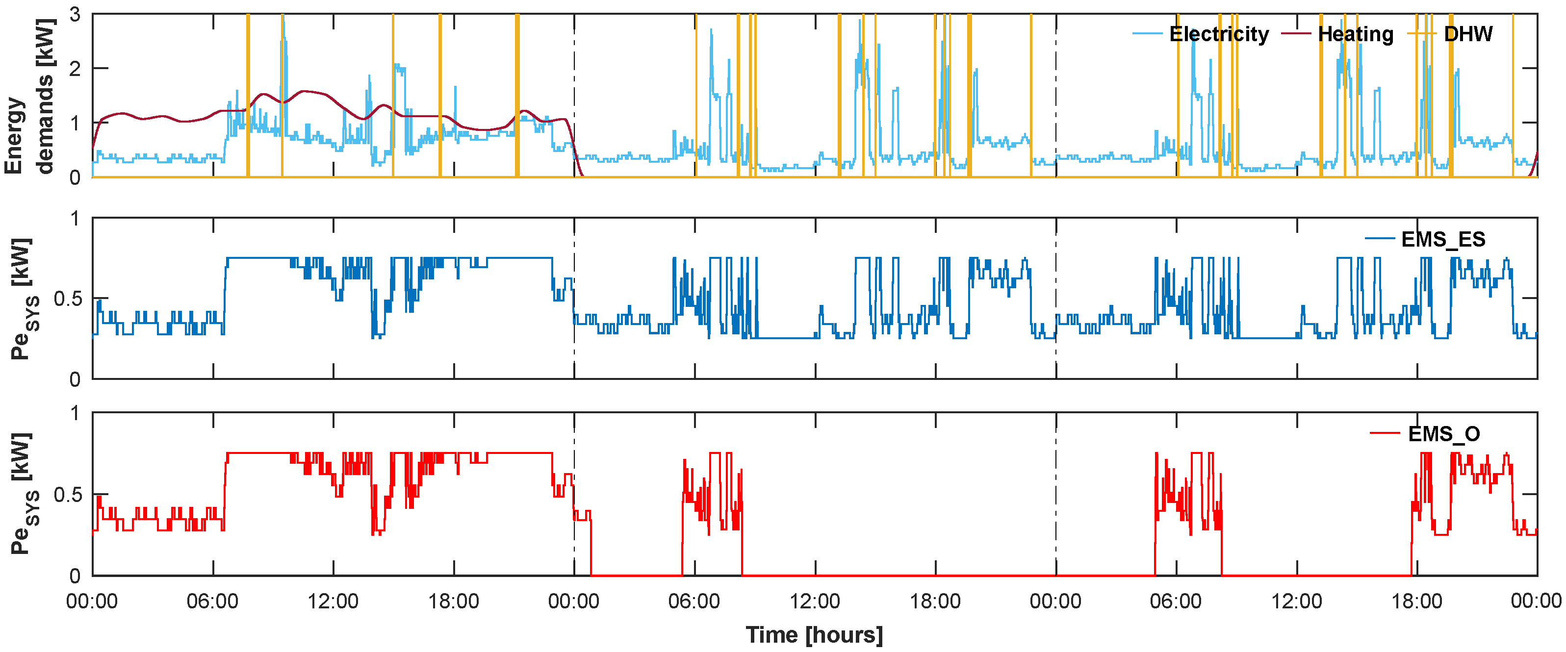
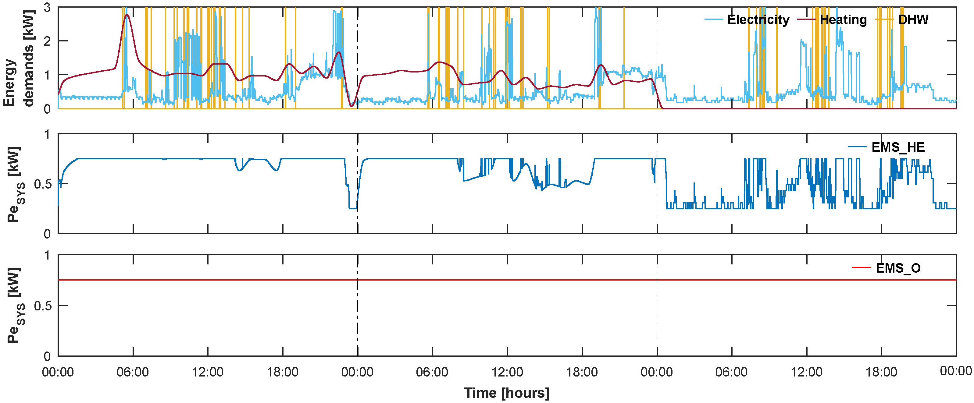
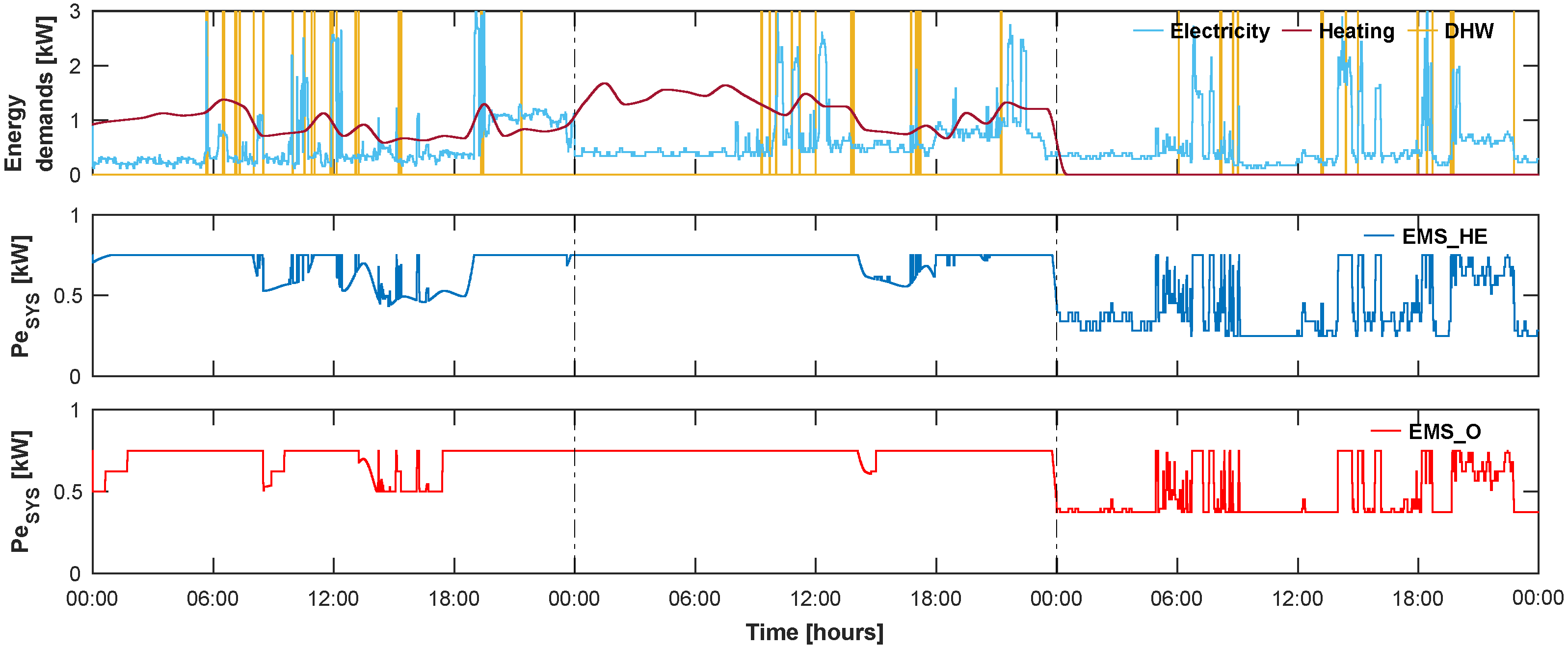
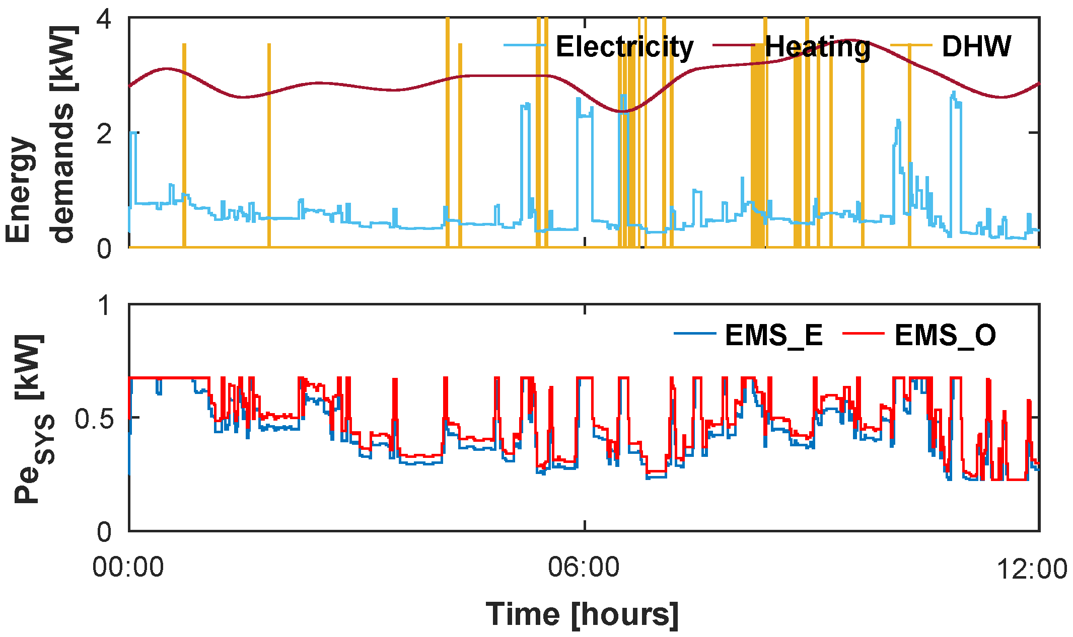
3.2. Investigation of the Behavior of the Optimal EMS

The similarity of the savings achieved by the optimal EMS and the best rule-based EMS in each scenario could indicate a similarity in their behaviors. To investigate this hypothesis, the signal $P{e}_{SY{S}_k\left(bRB\right)}$ (the best rule-based EMS) was compared with the signal $P{e}_{SY{S}_k\left(O\right)}$ (the optimal EMS). Additionally, the indicator $\Phi$ was calculated, which is the average absolute difference in percentage with respect to the stack nominal power ($P{e}_{SY{S}_N}$), Equation (35). S is the number of samples taken to calculate the indicator; when considering a whole year, S = 365 days × 1440 min/day (525,600 samples), and if the indicator is evaluated for one day, then S = 1440 samples. A value of $\Phi =0\%$ would indicate that the signals are identical, while a value of $\Phi =100\%$ would indicate a maximum difference between them within the possible range (0–0.75 kW). The values of $\Phi$ are listed in Table 4.

$$\Phi ={\displaystyle \frac{\frac{1}{S}{\sum }_{k=1}^S\left|P{e}_{SY{S}_k\left(bRB\right)}-P{e}_{SY{S}_k\left(O\right)}\right|}{P{e}_{SY{S}_N}}}\times 100$$

(35)

$\Phi$ is in the range of 0.7–25.1%, with an average value of 8.5%. In 35 out of 46 scenarios (76%), $\Phi \le 10.5\%$. These numbers confirm the hypothesis posed at the beginning of this section; indeed, they show that the strategy followed by the optimal EMS in each of the scenarios is (globally, i.e., when considering the entire year) similar to the strategy of the best rule-based EMS.

Now, the values of $\Phi$ in Table 4 do not provide any information about how the optimal EMS behaves locally, that is when considering a time window of hours. To obtain a more precise view of the (local) behavior of the optimal EMS and its similarity to the behavior of the best rule-based EMS, the signals from the 46 simulations were graphically represented, compared, and analyzed. Figure 7, Figure 8 and Figure 9 show three examples taken from this analysis.

The signals in Figure 7 belong to the simulation of scenario 3. On the first day, the EMS_O does almost the same as the best rule-based EMS (EMS_ES), namely, it follows the electricity demand. On the second and third days, the behavior of EMS_O is different from that of EMS_ES, but it either follows the electricity demand or turns off the micro-CHP system.

Figure 8 shows the signals from scenario 21. In this scenario, the best rule-based EMS is EMS_HE. Here, the behavior of EMS_O is different. It does not follow the electricity demand, nor the heat demand, nor the greater of the two: it sets the stack to maximum power.

Finally, Figure 9 shows the signals corresponding to scenario 20. Here, too, the best rule-based EMS is EMS_HE. On the first day, the behavior of EMS_O is similar to that of EMS_HE, although not exactly the same. The same occurs on the third day: EMS_O does something similar to what EMS_HE does (following the electricity demand, since there is no heat demand), but not exactly the same. In this last case, the difference lies in the minimum value to which the stack is set. Although its behavior on these two days is different, it shows a strong similarity to that of the best rule-based EMS, with $\Phi$ values of 5.9% and 6.9% for the first and third days, respectively.

An additional example of similar but not identical behavior to that of the best rule-based EMS is shown in Figure 10.

The complete analysis of the annual signals from the simulations in the 46 scenarios reveals that the optimal EMS does one of these five things (list of identified behaviors):

• Following the electricity demand.
• Following the greater of the demands, electricity and heat.
• Turning off the micro-CHP system.
• Setting the micro-CHP system to maximum power.
• Other behaviors that are similar but not identical to 1 or 2.

The reason that EMS_H achieves greater savings than EMS_HE in some scenarios (15, 36–39, Figure 3), despite following heat not being an optimal pattern, lies in the fact that the economic performances considered are annual, whereas when discussing optimal operating patterns, a local time window (hours) is assumed. In particular, in those scenarios, the following occurs: in summer, the most cost-effective approach is to turn off the system, and the behavior of EMS_H is closer to that pattern (since there is no heating demand) than that of EMS_HE, which follows electricity.

It is important to note that most of the behavioral differences quantified in the global $\Phi$ values (Table 4) are of the type shown in Figure 7 and Figure 8: distinct behaviors from each other but both equal to some of the first four identified behaviors. We will refer to these differences as type A behavioral differences. The rest of the behavioral differences are those specific to what has been termed “other behaviors” (item number 5 in the list of identified behaviors), that is, differences of the type shown in Figure 9 (first and third day) and in Figure 10. We will refer to these differences as type B behavioral differences.

An additional indicator, $\Psi$ (Equation (36)), was devised to provide numerical evidence of the stated fact, namely, that most of the behavioral differences quantified in the global $\Phi$ values are type A differences. In the calculation of $\Psi$, Equation (36), type A behavioral differences become zero, so that only type B behavioral differences contribute to the value of $\Psi$. The values of $\Psi$ are listed in Table 4.

$$\Psi ={\displaystyle \frac{\frac{1}{S}{\sum }_{k=1}^{S}min\left|P{e}_{SY{S}_k\left(j\right)}-P{e}_{SY{S}_k\left(O\right)}\right|}{P{e}_{SY{S}_N}}}\times 100\forall j\in \{E,HE,off,max\}$$

(36)

The range of $\Psi$ is 0–6.4% and its average value is 2.2%. From the average values of $\Phi$ and $\Psi$, it can be inferred that, globally (considering all 46 scenarios), 74% of the accumulated absolute difference (between the signal of the optimal EMS and that of the best rule-based EMS) is due to type A behavioral differences, while 26% corresponds to type B behavioral differences; in effect, ((8.5 − 2.2)/8.5) × 100 = 74%, and 100 − 74 = 26%.

Figure 11 shows the cumulative histograms of the differences in $\Phi$ and $\Psi$ (that is, the differences that contribute to the values of $\Phi$ and $\Psi$). In both cases, the number of differences represented is 24,177,600 (365 days × 1440 min/day × 46 scenarios). The cumulative histograms display how the differences are distributed.

The cumulative histogram of the differences in $\Phi$, Equation (35), shows that most of the differences are small: 78% of the differences in $\Phi$ are less than or equal to 75 W (10% of the nominal power of the stack). Consequently, this reaffirms that, in general, the behavior of the optimal EMS is similar to that of the best rule-based EMS.

In the cumulative histogram of the differences in $\Psi$, all differences are type B differences, since in the calculation of $\Psi$, type A differences become zero (see Equation (36)). Type B differences are significantly more densely distributed towards the lower end of the range. There are no type B differences greater than 350 W, while there are type A differences of up to 750 W: 99% of the type B differences fall within the range 0–125 W (17% of the nominal power of the stack), whereas for the same threshold, type A differences can reach up to 675 W (90% of the nominal power of the stack); 92% of the differences in $\Psi$ are less than or equal to 75 W (10% of the nominal power of the stack). This means that 92% of the differences specific of what has been termed “other behaviors” are less than 10% of the nominal power of the stack.

4. Discussion

The discussion is divided into two subsections: the first, Section 4.1, discusses the economic performance of the optimal EMS (third part of this contribution), and the second, Section 4.2, discusses its behavior (fourth part of this contribution).

4.1. Economic Performance of the Optimal EMS

For a given scenario, the savings achieved by the optimal EMS are small compared to the best rule-based EMS ($\Delta \le 2$ pp). This result is consistent with the data reported by Houwing et al. [18] (1 pp, scenario with a fixed tariff structure).

The savings reported by Hawkes et al. [17] (4 pp, case 2 kWe SOFC) is double that found here. This discrepancy could be due to our model taking into account certain physical phenomena that are neglected there, such as heat losses in the TES or the startup and shutdown costs (see Table 1, second block). Another possible explanation is that neither EMS_H nor EMS_E (with respect to which they calculate their figure) is the best of the rule-based EMS, but rather EMS_HE, which is not included in their comparison.

Shaneb et al. [20] report values significantly higher than those obtained in this study, namely, 15–22 pp for the electricity trading scenario, case FiT 100% (they do not provide their results in pp with respect to the operating cost of the reference system, the range provided is an estimate). The reason for this is most likely that their comparison did not include EMS_HE, which is indeed the best when FiT values are high, as demonstrated by the results in Figure 3. This highlights, as mentioned in the Introduction (Section 1), the great importance of including all four relevant rule-based EMS in the comparison. Only in this way can the economic performance of the optimal EMS be correctly evaluated in relation to the rule-based EMSs and a conclusive result be reached.

The reason that the optimal EMS achieves such a small savings compared to the best rule-based EMS likely lies in the fact that the energy management of micro-CHP systems has few degrees of freedom, especially when compared to other systems like hybrid renewable energy systems (HRESs), which typically have multiple generators and energy storage units.

This result, namely, the small benefit that the optimal EMS achieves compared to the best rule-based EMS in each scenario, might lead one to think that an optimal EMS is not worth it. This is indeed the opinion expressed in [12,17,18]. However, this conclusion would be hasty. The optimal EMS has a major advantage over the rule-based EMSs, namely, it is capable of adapting to changes of scenario. Navarro et al. [15] demonstrated that changes of scenario are frequent in micro-CHP (see Section 6.3, fourth paragraph) and that adapting the energy management strategy to the scenario can generate annual savings of up to 14.5 pp. In absolute terms, assuming an annual energy bill of EUR 2500 with the reference system, this translates to EUR 362. Over the lifetime of the system, therefore, this adaptability results in considerable economic savings.

Thus, it is not generally the case, as stated in Hawkes et al. [17], that there is little economic benefit in operating the micro-CHP system with an optimal EMS, in comparison with rule-based EMSs. This is only true if a fixed scenario is assumed (as is done in that study), which is an unrealistic assumption for micro-CHP systems today. Similarly, Staffell et al. [12], based on the results of Hawkes et al. [17], assumed in their study that the heat-and-electricity-led strategy produces economic savings close to those of an optimal EMS. Again, this is only true if a specific and fixed scenario is considered, not when there are scenario changes. For example, see the scenario change from 16 → 2 in Figure 3. Staffell’s assumption in [12] holds true in scenario 16 but is false in scenario 2.

In general, the importance of scenario changes has been overlooked in the studies conducted to date. Only when these are taken into account does the superiority of the optimal EMS over rule-based EMSs become evident. However, the optimal EMS also has significant drawbacks: it is complex, sensitive to errors in the predictions and the model, and has a high computational cost. The ideal solution, therefore, would be an EMS that is simultaneously capable of adapting to changing scenarios and is simple, robust, and fast. Such an EMS would achieve near-optimal global savings (i.e., considering the entire lifetime of the micro-CHP system). If such an EMS could be designed, then indeed, implementing an optimal EMS would not be worthwhile, given that (1) the difference in savings achieved by the latter compared to the former would be small, and (2) its disadvantages are significant. The analysis of the behavior of the optimal EMS, discussed in the following section, is a first step toward designing this new EMS.

4.2. Behavior of the Optimal EMS

The “other behaviors” are always very similar to behaviors 1 (following electricity demand) or 2 (following the greater of the electricity and heat demands) from the list of identified behaviors. This is inferred, on the one hand, from the analysis of the signals and the small values of $\Phi$ that result when these behaviors are compared locally (see, for example, Figure 9 and Figure 10, and the $\Phi$ values indicated in the captions of those figures) and, on the other hand, from the small values of $\Psi$. Furthermore, note that the “other behaviors” are not necessary to achieve near-optimal savings. Indeed, none of the rule-based EMSs operate according to these other behaviors, and yet they achieve savings very close to those of the optimal EMS ($\Delta \le 2$ pp). See, for example, the results in Figure 3.

If, based on these observations, the “other behaviors” are disregarded, the results presented in Section 3.2 show that the behavior of the optimal EMS can be reduced to four fundamental optimal operating patterns: (1) follow electricity, (2) follow electricity and heat, (3) turn off the system, and (4) operate at maximum power. This result partially agrees with the findings of Hawkes et al. [17] for an SOFC-based micro-CHP system. In their study, patterns (3) and (4) were not identified. The reason for this is presumably that they included a minimum load constraint (relevant for SOFC) and a limit on the amount of heat that could be dumped.

The optimal operating pattern strongly depends on the FiT. Compare, for example, scenarios 7 and 21 in Figure 3. This result exactly matches the findings of Hawkes et al. [17] (there, FiT is called electricity buyback rate). The optimal operating pattern also changes depending on the stack degradation level. Compare, for example, the following scenario changes due to changes in the degradation level, Figure 3: 4 → 25, 5 → 26, 11 → 32, 12 → 33, 16 → 37, 17 → 38, 18 → 39. This relationship between the optimal operating pattern and the level of degradation was not studied by Hawkes et al. [17].

The optimal operating pattern is also sensitive to fuel prices (spark gap). This is clearly seen in Figure 3 (FiT25, BOL). This result contradicts what was reported by Hawkes et al. [17], where it was concluded that prices (import energy prices) have little effect on the optimal operating pattern. The reason for this discrepancy likely lies in the difference in the range of spark gap considered: 3.15–4.53 (1.39) in Hawkes et al. [17] versus 2.85–5.77 (2.92) in this study. The range is more than twice as large in the present study. Their smaller spark gap range is due to their study being limited to the United Kingdom, whereas ours considers the European market, where price variability is greater.

In the studied framework (Europe) and under the assumed methodological assumptions, any of the four identified fundamental operating patterns can be optimal (or near-optimal), and only those four can be optimal (setting aside the “other behaviors”). This being the case, the problem of managing PEMFC-based micro-CHP systems comes down to this: choosing the most cost-effective of these four patterns for the given scenario.

For this task, a key question is what time window to use in characterizing the scenario. From the preliminary study conducted to determine the prediction horizon of the optimal EMS (Section 2.2), as well as from the running phase of the simulations performed to obtain the savings of the optimal EMS in the 46 scenarios, it is inferred that 8 h (HP 480 samples) is an adequate time window for this purpose. Indeed, the fact that the EMS_O does not achieve greater savings with longer prediction horizons proves that the information beyond this time window is irrelevant for selecting the optimal operating pattern.

An optimization horizon of 8 h is preferable to one day, which is the value chosen in the research conducted to date [17,18,19,20,21] (see Table 1, third block). The reason for this is that the shorter the window, the more reliable the demand prediction will be and, consequently, the more accurate the scenario characterization. This, in turn, will lead to a more accurate selection of the operating pattern. Indeed, in general, the probability of making an accurate prediction is higher for the near future than for the distant future—for example, as is the case with weather forecasting.

Finally, it must be said that a prediction horizon of eight hours is suitable for the micro-CHP system and the demand profiles considered in this study. These were chosen to represent the standard case [10,28], so that the results would have a certain generality. However, for systems with different TES sizes or in applications with significantly different energy demands, the appropriate prediction horizon could be longer or shorter than eight hours.

5. Conclusions

This study evaluated the operation of an optimal EMS for a PEMFC-based micro-CHP system under 46 scenarios representative of the European context. The analysis identified four fundamental optimal operating patterns: (1) follow electricity, (2) follow electricity and heat, (3) turn off the system, and (4) operate at maximum power. This categorization, not previously reported in the literature, constitutes the main contribution of the study.

These patterns demonstrate that the energy management of PEMFC-based micro-CHP systems can be effectively simplified without significant loss in economic performance. This finding enables the design of new EMS strategies that, while less complex than fully optimized approaches, achieve comparable cost-effectiveness. Such improvements have the potential to reduce payback periods and support broader commercialization of fuel cell micro-cogeneration technologies.

Additionally, results indicate that an eight-hour prediction horizon is sufficient to determine the appropriate operating pattern. This is notably shorter than those proposed in previous studies, offering a practical advantage by reducing forecasting uncertainty and computational burden.

Future work will primarily build upon the behavioral pattern analysis presented in this study, aiming to develop an energy management system (EMS) capable of selecting, in real time and based on the operational context, the most suitable operating strategy among the predefined patterns. This selection process will leverage artificial intelligence techniques to approximate optimal EMS performance while maintaining low computational complexity, thus enabling practical real-time application. In parallel, further research will explore the feasibility of implementing an optimal EMS based on hierarchical model predictive control (MPC), with a focus on achieving a balance between long-term planning and short-term responsiveness within the constraints of real-time platforms.

References

1. Dodds, P.E.; Staffell, I.; Hawkes, A.D.; Li, F.; Grünewald, P.; McDowall, W.; Ekins, P. Hydrogen and fuel cell technologies for heating: A review. Int. J. Hydrogen Energy 2015, 40, 2065–2083. [Google Scholar] [CrossRef]
2. van der Spek, M.; Banet, C.; Bauer, C.; Gabrielli, P.; Goldthorpe, W.; Mazzotti, M.; Munkejord, S.T.; Røkke, N.A.; Shah, N.; Sunny, N.; et al. Perspective on the hydrogen economy as a pathway to reach net-zero CO2 emissions in Europe. Energy Environ. Sci. 2022, 15, 1034–1077. [Google Scholar] [CrossRef]
3. Staffell, I.; Scamman, D.; Abad, A.V.; Balcombe, P.; Dodds, P.E.; Ekins, P.; Shah, N.; Ward, K.R. The role of hydrogen and fuel cells in the global energy system. Energy Environ. Sci. 2019, 12, 463–491. [Google Scholar] [CrossRef]
4. Li, Q.; Hao, Y.; Sun, L. Modeling and evaluation of a steam and power cogeneration system of proton exchange membrane fuel cell coupled high temperature heat pump. Chem. Eng. J. 2025, 505, 159432. [Google Scholar] [CrossRef]
5. European Commission Recognises Fuel Cells as a Strategic Net-Zero Technology. News Dated March 17, 2023. PACE. Available online: https://pace-energy.eu/fuel-cells-net-zero-technology/ (accessed on 16 December 2024).
6. PACE: Pathway to a Competitive European Fuel Cell Micro-Cogeneration Market. Available online: https://pace-energy.eu/ (accessed on 10 January 2025).
7. Korteweg, H. The Bridge to Large Scale Market Uptake. European-Wide Field Trials for Residential Fuel Cell Micro-Cogeneration. PACE: Pathway to a Competitive European Fuel Cell Micro-Cogeneration Market. Presentation Given on 26 April 2023. Available online: https://pace-energy.eu/what-role-for-fuel-cell-micro-chp-in-europes-future-energy-system/ (accessed on 10 January 2025).
8. Adam, A.; Fraga, E.S.; Brett, D.J. A modelling study for the integration of a PEMFC micro-CHP in domestic building services design. Appl. Energy 2018, 225, 85–97. [Google Scholar] [CrossRef]
9. Ang, S.M.C.; Fraga, E.S.; Brandon, N.P.; Samsatli, N.J.; Brett, D.J. Fuel cell systems optimization—Methods and strategies. Int. J. Hydrogen Energy 2011, 36, 14678–14703. [Google Scholar] [CrossRef]
10. Staffell, I. Fuel Cells for Domestic Heat and Power: Are They Worth It? Ph.D. Thesis, University of Birmingham, Birmingham, UK, 2010. [Google Scholar]
11. 6154104 GB 4/2020; Viessmann. Product Data sheet. Vitovalor PT2. Micro CHP Unit on Fuel Cell Basis with Integral Gas Condensing Boiler. Viessmann Werke GmbH & Co. KG, D-35107: Allendorf, Germany.
12. Staffell, I.; Green, R.; Kendall, K. Cost targets for domestic fuel cell CHP. J. Power Sources 2008, 181, 339–349. [Google Scholar] [CrossRef]
13. Ito, H. Economic and environmental assessment of residential micro combined heat and power system application in Japan. Int. J. Hydrogen Energy 2016, 41, 15111–15123. [Google Scholar] [CrossRef]
14. Löbberding, L.; Madlener, R. Techno-economic analysis of micro fuel cell cogeneration and storage in Germany. Appl. Energy 2019, 235, 1603–1613. [Google Scholar] [CrossRef]
15. Navarro, S.; Herrero, J.M.; Blasco, X.; Pajares, A. Rule-based energy management strategies for PEMFC-based micro-CHP systems: A comparative analysis. Heliyon 2024, 10, e37685. [Google Scholar] [CrossRef] [PubMed]
16. Bordons, C.; Garcia-Torres, F.; Ridao, M.A. Model Predictive Control of Microgrids; Springer Nature: Berlin/Heidelberg, Germany, 2020; ISBN 978-3-030-24569-6. [Google Scholar]
17. Hawkes, A.D.; Leach, M.A. Cost-effective operating strategy for residential micro-combined heat and power. Energy 2007, 32, 711–723. [Google Scholar] [CrossRef]
18. Houwing, M.; Negenborn, R.R.; De Schutter, B. Demand Response with Micro-CHP Systems; IEEE: Piscataway, NJ, USA, 2011; Volume 99, pp. 200–213. [Google Scholar] [CrossRef]
19. Hawkes, A.D.; Brett, D.J.L.; Brandon, N.P. Fuel cell micro-CHP techno-economics: Part 1—model concept and formulation. Int. J. Hydrogen Energy 2009, 34, 9545–9557. [Google Scholar] [CrossRef]
20. Shaneb, O.A.; Taylor, P.C.; Coates, G. Optimal online operation of residential μCHP systems using linear programming. Energy Build. 2012, 44, 17–25. [Google Scholar] [CrossRef]
21. Ren, H.; Gao, W. Economic and environmental evaluation of micro CHP systems with different operating modes for residential buildings in Japan. Energy Build. 2010, 42, 853–861. [Google Scholar] [CrossRef]
22. Alahäivälä, A.; Heß, T.; Cao, S.; Lehtonen, M. Analyzing the optimal coordination of a residential micro-CHP system with a power sink. Appl. Energy 2015, 149, 326–337. [Google Scholar] [CrossRef]
23. Mohammadi, H.; Mohammadi, M. Optimization of the micro combined heat and power systems considering objective functions, components and operation strategies by an integrated approach. Energy Convers. Manag. 2020, 208, 112610. [Google Scholar] [CrossRef]
24. Oh, S.D.; Kim, K.Y.; Oh, S.B.; Kwak, H.Y. Optimal operation of a 1-kW PEMFC-based CHP system for residential applications. Appl. Energy 2012, 95, 93–101. [Google Scholar] [CrossRef]
25. Ozawa, A.; Kudoh, Y. Performance of residential fuel-cell-combined heat and power systems for various household types in Japan. Int. J. Hydrogen Energy 2018, 43, 15412–15422. [Google Scholar] [CrossRef]
26. Hawkes, A.D.; Aguiar, P.; Hernandez-Aramburo, C.A.; Leach, M.A.; Brandon, N.P.; Green, T.C.; Adjiman, C.S. Techno-economic modelling of a solid oxide fuel cell stack for micro combined heat and power. J. Power Sources 2006, 156, 321–333. [Google Scholar] [CrossRef]
27. Ren, H.; Gao, W.; Ruan, Y. Optimal sizing for residential CHP system. Appl. Therm. Eng. 2008, 28, 514–523. [Google Scholar] [CrossRef]
28. VDI. Referenzlastprofile von Ein- und Mehrfamilienhäusern für den Einsatz von KWK-Anlagen: [Eng: Reference load Profiles of Single-Family and Multi-Family Houses for the Use of CHP Systems]; 27.100, 91.140.10(4655); Beuth Verlag: Düsseldorf, Germany, 2008. [Google Scholar]
29. Sánchez, E.P.P. Desarrollo de un Sistema de Gestión de Energía Eléctrica y Térmica en Viviendas Unifamiliares (Micro-CHP) con Pilas de Combustible. Master’s Thesis, Universitat Politècnica de València, Valencia, Spain, 2019. Available online: http://hdl.handle.net/10251/129431 (accessed on 11 May 2025).
Figure 1. Micro-CHP system [15].
Applsci 15 07527 g001
Figure 2. Results of the preliminary study conducted to determine the HP. The sequences are WWF WWC WWC (winter), TWF TWF TWC (transition), and SWX SWX SWX (summer).
Applsci 15 07527 g002
Figure 3. Economic performance of the optimal EMS compared to those achieved by the rule-based EMSs, in 42 out of the 46 simulated scenarios. The colored rectangles indicate which of the rule-based EMSs is the best.
Applsci 15 07527 g003
Figure 4. Economic performance of the optimal EMS compared to those achieved by the rule-based EMSs, scenarios 43 and 44. Effect of a change in the HPR of the demand.
Applsci 15 07527 g004
Figure 5. Economic performance of the optimal EMS compared to those achieved by the rule-based EMSs, scenarios 45 and 46. Effect of a change in climate zone.
Applsci 15 07527 g005
Figure 6. Histogram of Δ .
Applsci 15 07527 g006
Figure 7. Behavior of the optimal EMS. Example No. 1: Scenario 3. Start: Day 157. Window: 3 days. Sequence: TSC SWX SWX. First day: Φ 0.1%. Second day: Φ 45.5%. Third day: Φ 28.6%.
Applsci 15 07527 g007
Figure 8. Behavior of the optimal EMS. Example No. 2: Scenario 21. Start: Day 169. Window: 3 days. Sequence: TWC TWF SSX. First day: Φ 4.2%. Second day: Φ 10.3%. Third day: Φ 42.1%.
Applsci 15 07527 g008
Figure 9. Behavior of the optimal EMS. Example No. 3: Scenario 20. Start: Day 240. Window: 3 days. Sequence: TWF TSF SWX. First day: Φ 5.9%. Second day: Φ 2.3%. Third day: Φ 6.9%, minimum values, EMS_HE 0.250 kW, EMS_O 0.374 kW.
Applsci 15 07527 g009
Figure 10. Behavior of the optimal EMS. Additional example: Scenario 28. Start: Day 4. Window: 12 h. Day WWC. Φ = 5.5 % .
Applsci 15 07527 g010
Figure 11. Cumulative histograms of the differences in Φ and Ψ .
Applsci 15 07527 g011