Author Contributions
Conceptualization, all authors; methodology, C.Z. and J.Z.; software, C.Z. and M.F.; validation, J.Z. and Y.C.; formal analysis, M.F. and Y.C.; investigation, C.Z. and M.F.; resources, Y.L.; data curation, M.F.; writing—original draft preparation, C.Z.; writing—review and editing, C.Z. and Y.L.; visualization, J.Z. and Y.C.; supervision, Y.L. and C.W.; project administration, Y.L. and C.W.; funding acquisition, Y.L. and C.W. All authors have read and agreed to the published version of the manuscript.
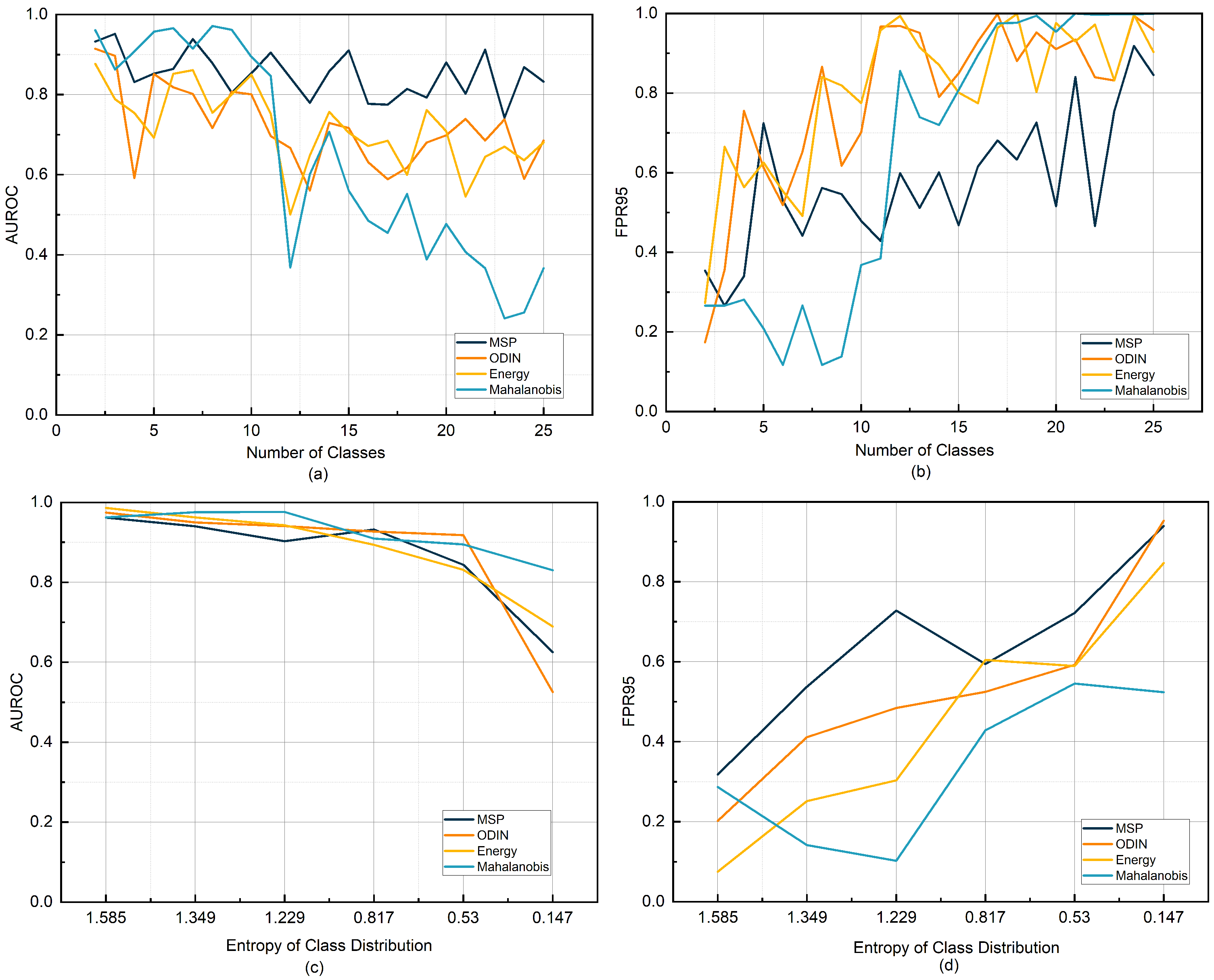
Figure 1.
Variation in OOD detection performance (AUROC/FPR95) under different class numbers and imbalance levels on the CIC IoT 2022 dataset. (a,b) show the changes in AUROC and FPR95 as the number of in-distribution classes increases. (c,d) present the changes in AUROC and FPR95 as the in-distribution class imbalance increases.
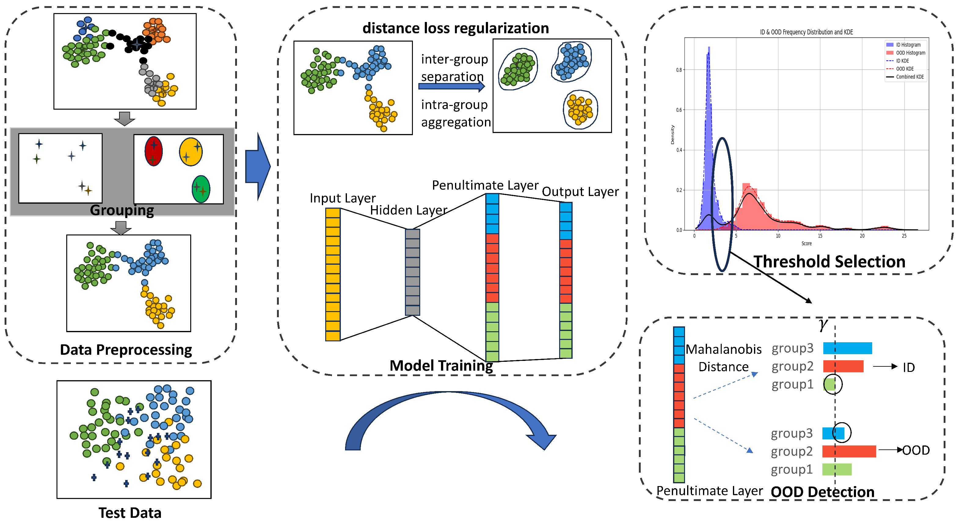
Figure 2.
Workflow of ODDL. The model clusters training data based on class means and applies a feature distance loss to optimize penultimate-layer representations, enhancing intra-group compactness and inter-group separability. At inference, Mahalanobis distances to each group are computed, and the maximum distance is used as the OOD score. An adaptive threshold is selected using KDE by locating local minima in the score distribution. Samples exceeding this threshold are classified as OOD.
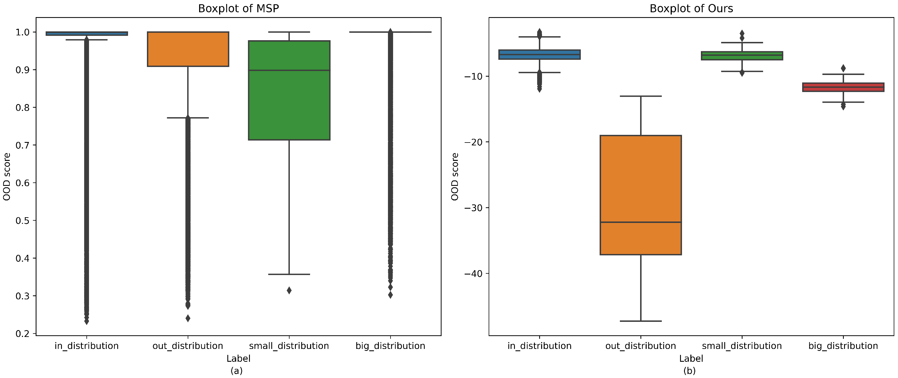
Figure 3.
Comparison of OOD score distributions. Boxplots of OOD scores produced by MSP and our proposed method for in-distribution (ID) samples, out-of-distribution (OOD) samples, a minority class, and a majority class. (a) shows the distribution under MSP, which tends to misclassify minority classes as OOD and fails to detect some true OOD samples. (b) shows the distribution under our method, which more effectively separates ID and OOD samples despite class imbalance.
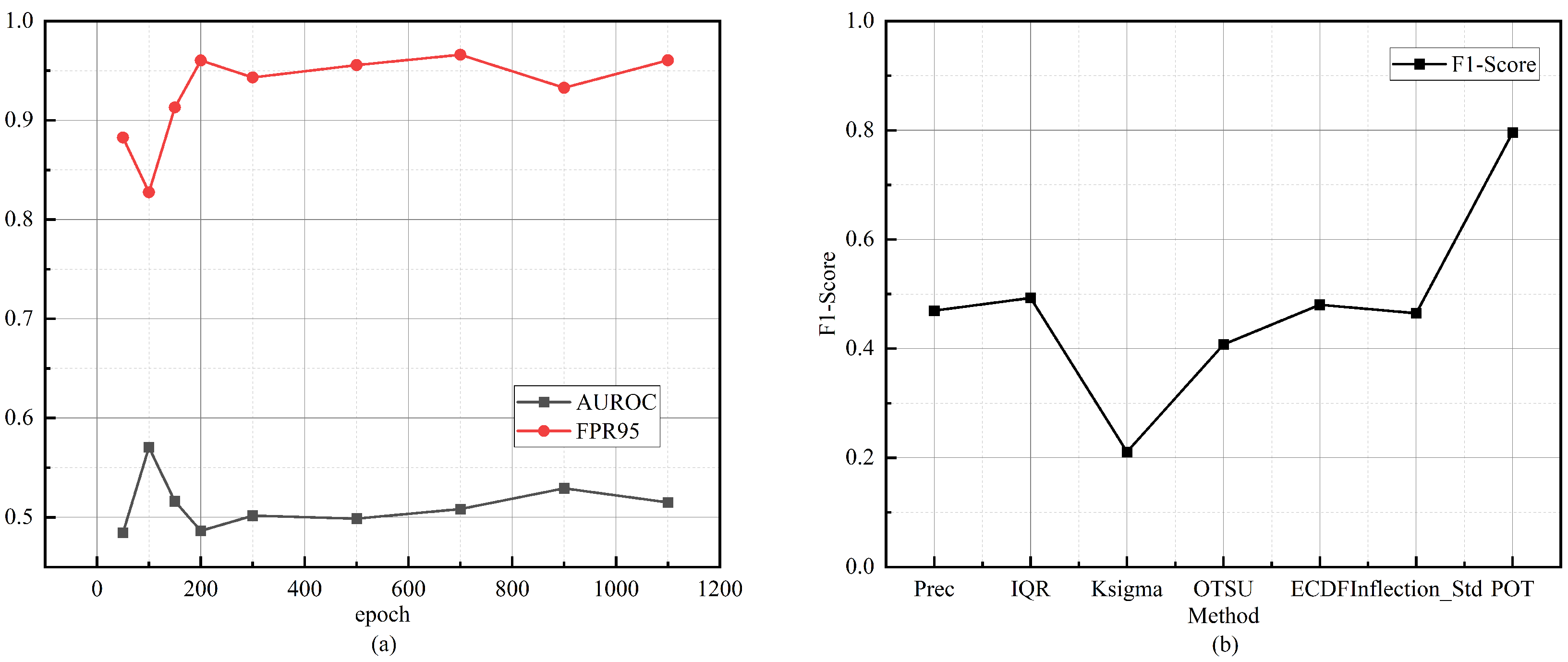
Figure 4.
OOD detection performance. (a) Variation in AUROC and FPR95 as training epochs increase. Performance first improves and then degrades, indicating overfitting in later training stages. (b) Comparison of different threshold selection strategies within our framework. The performance disparity highlights the need for an adaptive thresholding mechanism to ensure consistent OOD detection.
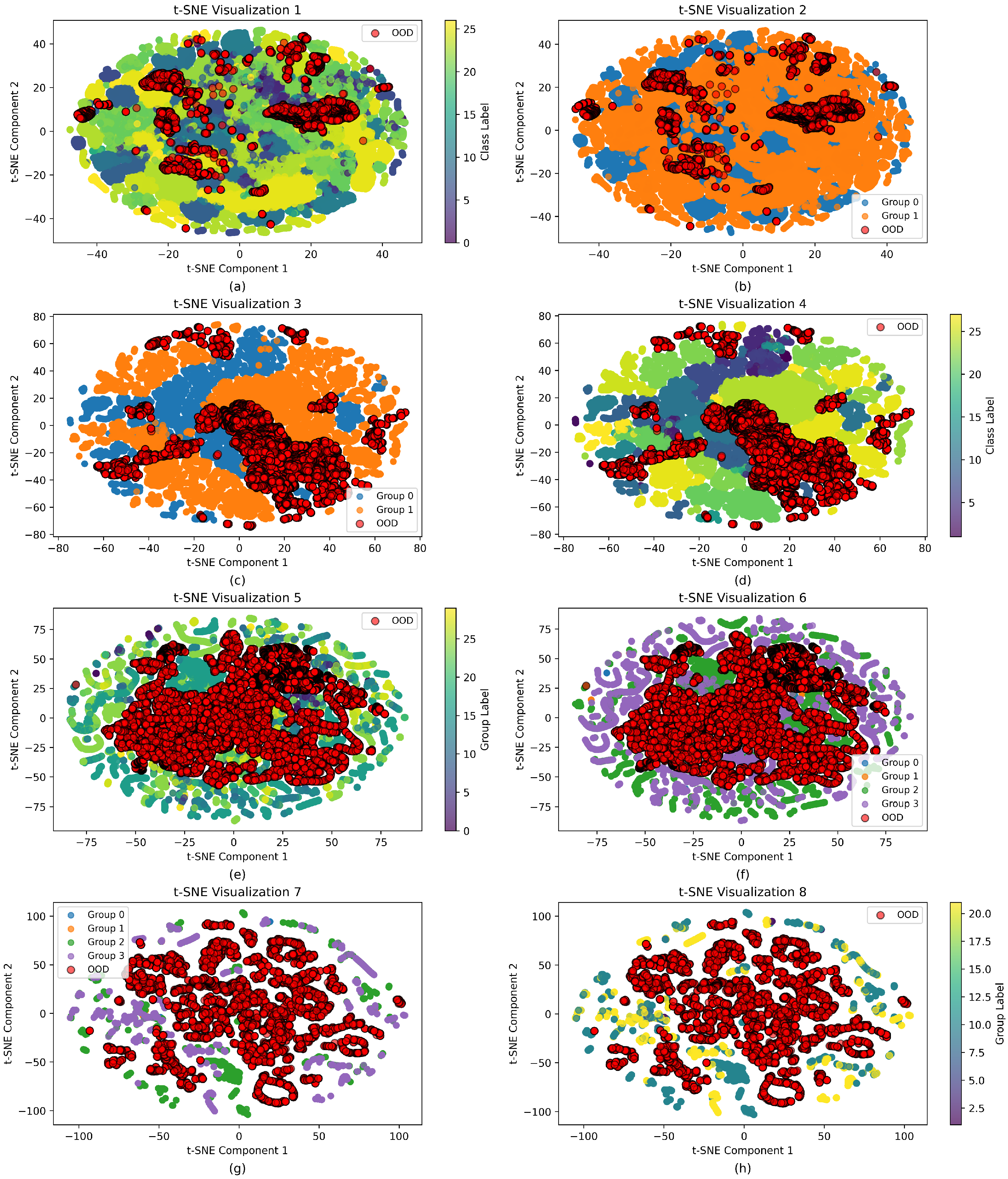
Figure 5.
t-SNE visualization of feature distributions for two OOD detection scenarios. (a–d) CIC IoT 2022 dataset with the Amcrest device as OOD. (a) Raw class features. (b) Group features after class mean-based clustering. (c) Group features after distance loss optimization. (d) Class features after distance loss optimization. (e–h) IoT Sentinel dataset with the grid TTU device as OOD, corresponding to feature representations in (a–d).
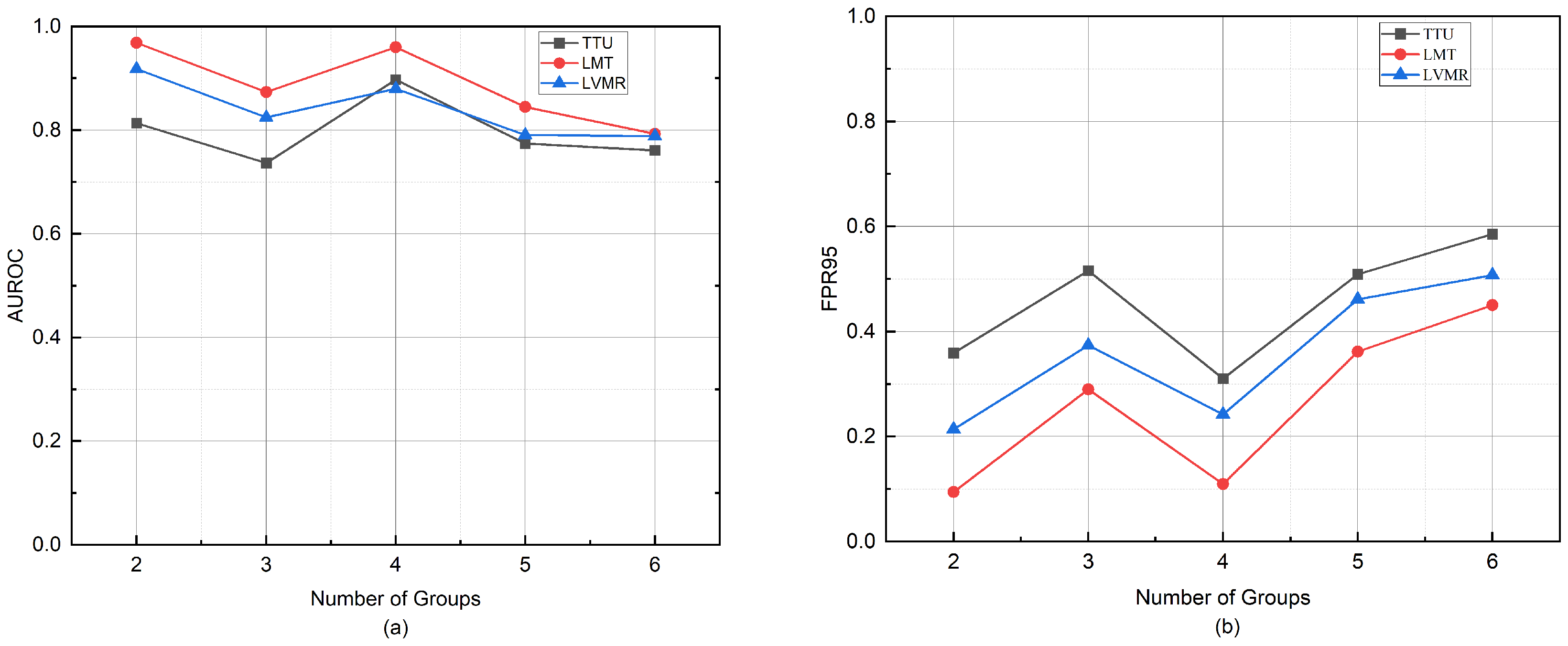
Figure 6.
Impact of different group numbers on OOD detection performance measured by AUROC and FPR95, using IoT Sentinel as the in-distribution dataset and Shenzhen power grid traffic as the OOD dataset. (a) shows the AUROC variation with increasing group numbers. (b) shows the corresponding FPR95 changes.
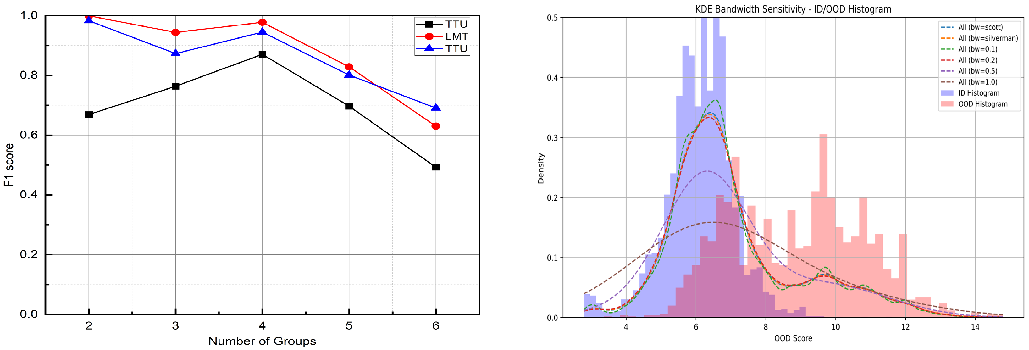
Figure 7.
Sensitivity analysis of key hyperparameters in the proposed OOD detection framework. Left: The effect of varying the number of groups on the F1 score under the KDE-based thresholding strategy. Results are obtained from the IoT dataset. Right histogram of OOD detection scores for in-distribution (ID, in blue) and out-of-distribution (OOD, in red) test samples. Overlaid Kernel density estimation (KDE) curves illustrate the effect of different bandwidth values (h) on score distribution smoothness. Larger bandwidths (e.g., or ) lead to over-smoothing and reduced separability between ID and OOD samples.
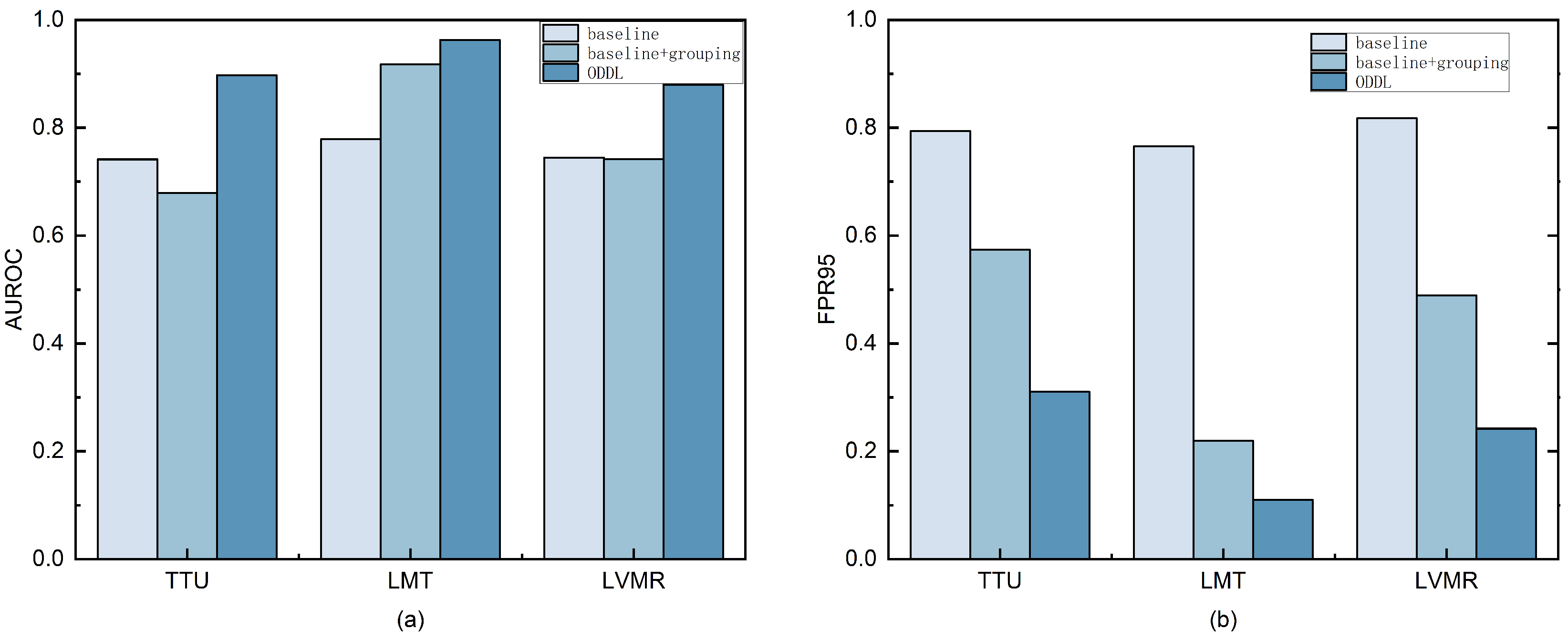
Figure 8.
Ablation study results on different OOD test sets. Each bar group represents the performance of three configurations: (1) Baseline (only cross-entropy loss), (2) Baseline + Grouping, and (3) Baseline + Grouping + Distance Loss (ODDL). (a) shows the AUROC results, and (b) shows the FPR95 results across the different OOD test sets. The figure illustrates the incremental effect of the grouping and distance loss modules in improving OOD detection performance.
Figure 9.
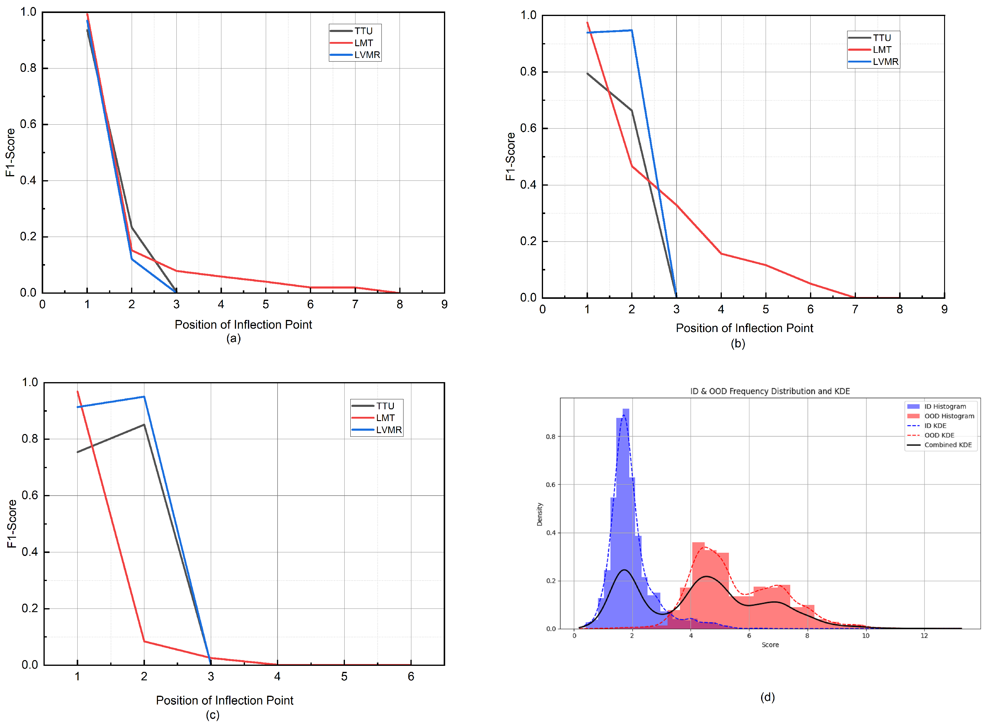
Comparison of F1 scores at different inflection points for the KDE-based adaptive threshold selection method. (a–c) show the F1 scores on different OOD test sets at various inflection points. (d) presents the KDE smoothing estimate of the OOD scores on the test set, with histograms of the ID (blue) and OOD (red) sample scores.
Figure 9.
Comparison of F1 scores at different inflection points for the KDE-based adaptive threshold selection method. (a–c) show the F1 scores on different OOD test sets at various inflection points. (d) presents the KDE smoothing estimate of the OOD scores on the test set, with histograms of the ID (blue) and OOD (red) sample scores.
Table 1.
Sample distribution of the CIC IoT Dataset 2022, collected from 28 different IoT devices. The table shows the number of samples per device, highlighting the dataset’s diversity in terms of traffic patterns and device types.
Table 1.
Sample distribution of the CIC IoT Dataset 2022, collected from 28 different IoT devices. The table shows the number of samples per device, highlighting the dataset’s diversity in terms of traffic patterns and device types.
| Device Type | Device Name | Number of Samples |
|---|
| Audio | echodot | 2786 |
| echospot | 3218 |
| echostudio | 2932 |
| nestmini | 3269 |
| sonos | 6569 |
| Camera | amcrest | 18,362 |
| arlobasecam | 20,520 |
| arloqcam | 21,948 |
| boruncam | 2432 |
| dlinkcam | 14,099 |
| heimvisioncam | 13,787 |
| homeyecam | 27,619 |
| luohecam | 20,076 |
| nestcam | 7490 |
| netatmcam | 10,625 |
| simcam | 34,217 |
| Home Automation | amazonplug | 584 |
| atomiccoffeemaker | 413 |
| eufyhomebase | 11,007 |
| globelamp | 908 |
| heimvisionlamp | 3813 |
| philips hue | 919 |
| roomba | 1106 |
| smartboard | 116 |
| teckin1 | 220 |
| teckin2 | 249 |
| yutron1 | 239 |
| yutron2 | 234 |
Table 2.
Distribution of samples in power grid traffic.
Table 2.
Distribution of samples in power grid traffic.
| Terminal Category | Function Description | Number of Samples |
|---|
| TTU | Monitor and record the operating conditions of distribution transformers | 226 |
| LMT | Terminal used for on-site service and management with functions such as remote metering reading and energy monitoring | 3056 |
| LVMR | Receive and forward commands from the master station to collect and control data from electric energy meters | 833 |
Table 3.
Comparison of OOD detection performance between our method and baseline methods on the CIC IoT Dataset 2022. All values represent the average performance when each class is individually considered as an OOD sample, as detailed in
Section 4.1. For our method, we additionally report the standard deviation across multiple runs to assess performance stability. ↑ indicates that higher values are better, while ↓ indicates that lower values are preferred. The best-performing method is highlighted in bold.
| Method | CIC IoT Dataset 2022 |
|---|
| AUROC↑ | AUPR↑ | FPR95↓ | Inference Time (s) |
|---|
| MSP | 0.4918 | 0.8460 | 0.9798 | 3.3157 |
| AE | 0.3626 | 0.8536 | 0.9899 | 0.9031 |
| ODIN | 0.2889 | 0.8442 | 0.9603 | 2.0252 |
| Energy | 0.3317 | 0.8187 | 0.9477 | 0.7935 |
| Mahalanobis | 0.6027 | 0.8895 | 0.8005 | 2.9780 |
| Ours | 0.9905 ± 0.0151 | 0.9997 ± 0.0002 | 0.03047 ± 0.0482 | 0.04324 |
Table 4.
Comparison of OOD detection performance between our method and baseline methods using the open-source IoT Sentinel dataset as ID samples and the real power grid traffic dataset as OOD samples. All results represent the average over 10 independent runs under identical conditions. For our method, we additionally report the standard deviation to assess performance stability. ↑ indicates that higher values are better, and ↓ indicates that lower values are better. The best-performing method is highlighted in bold.
| Method | TTU | LMT | LVMR |
|---|
| AUROC↑ | FPR95↓ | AUROC↑ | FPR95↓ | AUROC↑ | FPR95↓ |
|---|
| MSP | 0.7415 | 0.7942 | 0.7790 | 0.7654 | 0.7447 | 0.8177 |
| AE | 0.5173 | 0.8991 | 0.5657 | 0.9705 | 0.4250 | 0.9577 |
| ODIN | 0.7922 | 0.6418 | 0.8187 | 0.6111 | 0.7876 | 0.6460 |
| Energy | 0.7650 | 0.6784 | 0.7348 | 0.6755 | 0.7280 | 0.7222 |
| mahalanobis | 0.1733 | 0.9726 | 0.1290 | 0.9896 | 0.1775 | 0.9628 |
| Ours | 0.8976 ± 0.0730 | 0.3104 ± 0.0828 | 0.9629 ± 0.0126 | 0.1097 ± 0.0702 | 0.8800 ± 0.0120 | 0.2421 ± 0.0599 |
Table 5.
F1 scores of OOD detection using different threshold selection strategies with IoT Sentinel as in-distribution samples and Shenzhen power grid traffic as OOD samples. For our method, we report the average and standard deviation of F1 scores over 10 independent runs to evaluate robustness.
Table 5.
F1 scores of OOD detection using different threshold selection strategies with IoT Sentinel as in-distribution samples and Shenzhen power grid traffic as OOD samples. For our method, we report the average and standard deviation of F1 scores over 10 independent runs to evaluate robustness.
| Method | TTU | LMT | LVMR |
|---|
| Prec | 0.873178 | 0.9689 | 0.932345 |
| IQR | 0.850899 | 0.941543 | 0.864865 |
| Ksigma | 0.636895 | 0.871205 | 0.649914 |
| OTSU | 0.881939 | 0.44696 | 0.9344 |
| ECDF | 0.705876 | 0.381533 | 0.47022 |
| Inflection_Std | 0.714447 | 0.961106 | 0.867697 |
| POT | 0.828682 | 0.576437 | 0.705651 |
| Ours | 0.870305 ± 0.0156 | 0.977578 ± 0.0220 | 0.944754 ± 0.0331 |
Table 6.
F1 scores for OOD detection using different threshold selection strategies, with Amcrest as the OOD sample and the remaining devices as ID samples on the CIC IoT Dataset 2022. For our method, the result is reported as the average ± standard deviation over five independent runs to assess robustness.
| Method | Amcrest |
|---|
| Prec | 0.895544 |
| IQR | 0.9808 |
| Ksigma | 0.987398 |
| OTSU | 0.91543 |
| ECDF | 0.79554 |
| Inflection_Std | 0.594377 |
| POT | 0.753772 |
| Ours | 0.989546 ± 0.0043 |
Table 7.
Comparison of inference times (in seconds) for various OOD detection methods on the CIC IoT 2022 and IoT Sentinel datasets. Lower values represent better runtime performance.
Table 7.
Comparison of inference times (in seconds) for various OOD detection methods on the CIC IoT 2022 and IoT Sentinel datasets. Lower values represent better runtime performance.
| Method | CIC IoT 2022 | IoT Sentinel |
|---|
| MSP | 3.3157 | 0.7098 |
| AE | 2.0252 | 0.6448 |
| ODIN | 0.7935 | 0.2821 |
| Energy | 0.9031 | 0.1961 |
| Mahalanobis | 2.9780 | 1.3786 |
| Ours | 0.04324 | 0.0111 |
Table 8.
Robustness evaluation under Gaussian noise () on the CIC-IoT2022 dataset. Metric: AUROC.
Table 8.
Robustness evaluation under Gaussian noise () on the CIC-IoT2022 dataset. Metric: AUROC.
| Method | No Noise (Clean) | Gaussian Noise |
|---|
| MSP | 0.4918 | 0.5650 |
| AE | 0.3626 | 0.5243 |
| ODIN | 0.2889 | 0.3196 |
| energy | 0.3317 | 0.3142 |
| Mahalanobis | 0.6027 | 0.4570 |
| Ours (ODDL) | 0.9905 ± 0.0151 | 0.9312 ± 0.0466 |
Table 9.
AUROC and FPR95 performance on the IoT-23 dataset. In each trial, one class is selected as the OOD class. Despite the large scale and class imbalance, our method consistently outperforms the baselines.
Table 9.
AUROC and FPR95 performance on the IoT-23 dataset. In each trial, one class is selected as the OOD class. Despite the large scale and class imbalance, our method consistently outperforms the baselines.
| Method | AUROC | FPR95 |
|---|
| MSP | 0.5352 | 0.9874 |
| ODIN | 0.4514 | 0.9986 |
| Energy | 0.5001 | 0.9987 |
| Ours | 0.8176 | 0.3365 |


 ,
, 
