Physics-Informed Neural Networks for Enhanced State Estimation in Unbalanced Distribution Power Systems

Abstract

State estimation in distribution power systems is increasingly challenged by the proliferation of distributed energy resources (DERs), bidirectional power flows, and the growing complexity of unbalanced network topologies. Physics-Informed Neural Networks (PINNs) offer a compelling solution by integrating machine learning with the physical laws that govern power system behavior. This paper introduces a PINN-based framework for state estimation in unbalanced distribution systems, leveraging available data and embedded physical knowledge to improve accuracy, computational efficiency, and robustness across diverse operating scenarios. The proposed method is evaluated on four IEEE test feeders—IEEE 13, 34, 37, and 123—using synthetic datasets generated via OpenDSS to emulate realistic operating scenarios, and demonstrates significant improvements over baseline models. Notably, the PINN achieves up to a 97% reduction in current estimation errors while maintaining high voltage prediction accuracy. Extensive simulations further assess model performance under noisy inputs and partial observability, where the PINN consistently outperforms conventional data-driven approaches. These results highlight the method’s ability to generalize under uncertainty, accelerate convergence, and preserve physical consistency in simulated real-world conditions without requiring large volumes of labeled training data.

1. Introduction

State estimation (SE) is a foundational function in power system monitoring and control, enabling operators to infer the complete state of the grid—typically bus voltage magnitudes and angles—from limited and potentially noisy measurements [1]. In distribution power systems, accurate state estimation has become increasingly critical with the proliferation of distributed energy resources (DERs), electric vehicles, and other smart grid technologies that introduce bidirectional power flows, stochastic behaviors, and operational uncertainties [2].

Traditionally, state estimation (SE) in power systems has been performed using the weighted least squares (WLS) method, a widely adopted approach due to its simplicity and robustness for transmission networks [3]. However, applying WLS to distribution systems—known as distribution system state estimation (DSSE)—faces significant challenges. These arise from characteristics unique to distribution networks, such as radial or weakly meshed topologies, lack of real-time measurements, low resistance-to-reactance (R/X) ratios, and sparse measurement infrastructure [4,5]. Additionally, distribution systems are typically unbalanced and require full three-phase modeling to capture their operating conditions accurately. Conventional SE approaches, which often assume balanced conditions, can produce inaccurate results when applied to these networks. The increasing integration of distributed energy resources (DERs) further complicates observability and introduces higher variability into the system [6,7]. These challenges have led to the development of specialized DSSE methods, including branch current-based state estimation, node voltage-based approaches, and methods leveraging pseudo-measurements derived from historical load data or load forecasts [8]. Despite these efforts, conventional DSSE methods frequently suffer from reduced accuracy and increased computational burden as network complexity scales.

In response, researchers have turned to machine learning (ML) approaches that can directly learn the mapping from measurements to system states. Enabled by advances in smart meters and phasor measurement units (PMUs), ML models offer faster inference and adaptability [9]. In response, researchers have turned to machine learning (ML) approaches that can directly learn the mapping from measurements to system states. Enabled by advances in smart meters and phasor measurement units (PMUs), ML models offer faster inference and adaptability [10]. However, purely data-driven methods often fail to incorporate the underlying physical principles of power systems, potentially leading to physically implausible results, especially when confronted with scenarios outside their training distributions [11]. Moreover, they require large volumes of labeled training data, which may not be available across diverse distribution network configurations.

Physics-Informed Neural Networks (PINNs) present a promising alternative that bridges the gap between purely data-driven and physics-based methods [12]. PINNs incorporate the governing equations of physical systems—such as the power flow equations—directly into the training objective of a neural network. This is achieved by augmenting the loss function with residuals of these equations, penalizing deviations from physical laws during training. By enforcing physical consistency, PINNs can generalize better in data-scarce settings, yielding solutions that conform to known operational constraints even in the absence of extensive labeled datasets [13].

Originally developed for solving partial differential equations in fluid mechanics and continuum physics, PINNs have been successfully adapted for several power system tasks. In the domain of power system dynamics and stability, PINNs have been applied to transient stability analysis, offering computational advantages over traditional numerical integration methods [13,14]. In the realm of power flow analysis, PINNs have shown promise for accelerating AC power flow calculations. A study by Eeckhout et al. [11] proposed an improved PINN-based AC power flow model for distribution networks that incorporates physical line losses, resulting in higher accuracy and increased learning potential. The authors demonstrated that their physics-informed approach outperformed conventional methods and exhibited strong prediction capabilities for scenarios outside the training set, addressing a substantial deficiency of purely model-free techniques.

The recent literature has increasingly focused on integrating physical modeling with machine learning to enhance SE in power systems [15]. PINNs have been explored for power systems by researchers like Misyris et al. [16], who demonstrated that embedding the AC power flow equations into neural networks enables better generalization under sparse measurement conditions. Falas et al. [2] proposed a PINN framework for accelerating state estimation tasks in distribution systems, reducing convergence time while maintaining physical consistency. The study demonstrated impressive results, achieving up to an 11% increase in accuracy, 75% reduction in the standard deviation of results, and 30% faster convergence, as validated through comprehensive experiments on the IEEE 14-bus system. Similarly, in [17], Zamzam and Sidiropoulos introduced physics-aware models that maintain observability even with limited data, addressing challenges typical in real-world networks. Tran et al. [18] further advanced this line of work by proposing a decentralized pruned physics-aware neural network (D-P2N2), which combines physical topology information and decentralized learning to improve scalability, computational efficiency, and accuracy in large-scale distribution grids. Other approaches, such as those by Ostrometzky et al. [19], highlight the ability of PINNs to maintain robustness under partial observability and measurement noise. These methods represent a shift from black-box learning to hybrid modeling, leveraging prior knowledge to mitigate overfitting and improve extrapolation in unseen operational regimes [20].

Graph-based architectures have also emerged as powerful tools for modeling electrical networks [21]. Donon et al. [22] and Lin et al. [8] developed message-passing neural networks tailored for power flow problems, capturing network topology and improving accuracy in both state estimation and power flow prediction. Building on this, Pagnier and Chertkov [23] introduced Physics-Informed Graphical Neural Networks (PIGNNs) that incorporate Kirchhoff’s laws directly into graph-based architectures, improving reliability in low-measurement regimes. More recently, Ngo et al. [24] proposed a hybrid GNN-PINN framework for three-phase unbalanced systems, offering improved scalability and accuracy in complex distribution networks. These advances collectively demonstrate that combining physical laws with deep learning not only addresses the limitations of purely data-driven models—such as lack of physical interpretability and poor generalization—but also provides a promising foundation for state estimation in increasingly complex and unbalanced distribution systems.

Despite the promising progress in recent studies, several critical research gaps remain in the application of PINNs to distribution system state estimation. Most existing works are either limited to transmission-level systems or assume simplified balanced conditions [2,10,22], overlooking the unique challenges posed by unbalanced, three-phase distribution networks. Furthermore, comprehensive benchmarking across multiple test feeders is often lacking [11,17,19], and performance under realistic conditions—such as measurement noise and partial observability—is not often explored in depth [11,24]. This paper addresses these gaps by developing a PINN-based framework specifically tailored for unbalanced distribution systems and systematically evaluating it on four IEEE benchmark feeders: IEEE13, IEEE34, IEEE37, and IEEE123. In contrast to previous studies that focus on balanced or transmission-level systems, the proposed approach explicitly handles multi-phase unbalanced networks and is validated across diverse grid topologies and operating conditions. The model’s performance is assessed not only in noise-free conditions but also under corrupted inputs and incomplete measurement scenarios—two realistic challenges often overlooked in prior PINN applications. Comparative analysis against baseline machine learning models highlights the superior accuracy, robustness, and generalization capabilities of the proposed PINN approach, providing valuable insights into its practical applicability for real-world distribution network monitoring.

2. Materials and Methods

The overall methodology consists of four main stages: (1) dataset generation via OpenDSS simulations with randomized load conditions; (2) robust preprocessing and normalization of complex quantities; (3) training of the PINN model using a combined voltage- and physics-based loss; and (4) evaluation across multiple test feeders under varying conditions including noise and partial observability.

2.1. State Estimation in Distribution Power Systems

This section provides the mathematical formulation of the state estimation problem in unbalanced distribution systems, laying the foundation for the PINN approach developed in this work. By formalizing the relationship between nodal power injections and bus voltages, we clarify the physical model that underpins the data generation process and informs the physics-based loss function used during PINN training.

In conventional DSSE, the system state comprises the complex voltage phasors at each bus. These are inferred from available measurements—such as power flows, voltage magnitudes, current values, or pseudo-measurements derived from historical data—using power flow equations and statistical estimation methods. These measurements are typically gathered from SCADA systems, smart meters, or forecasting models. In this work, however, we assume full knowledge of power injections per phase derived from simulated load profiles, which serve as direct inputs to the PINN.

In unbalanced three-phase distribution networks, the physical relationships between voltages and power injections must be modeled per phase. The complex power injection at bus $i$, phase $\varphi \in \{a, b, c\}$, is given by:

$$S_i^{\phi }=V_i^{\phi }·{\left(\sum _i\sum _{\psi }{Y}_{ij}^{\phi \psi }·V_j^{\psi }\right)}^{*}$$

(1)

where $S_i^{\phi }$ is the complex power injection, $V_i^{\phi }$ is the complex voltage at bus $i$—phase $\phi$, and $Y_{ij}^{\phi \psi }$ is the element of the three-phase nodal admittance matrix coupling phase $\phi$ of bus $i$ with phase $\psi$ of bus $j$. The active and reactive power components are obtained from the real and imaginary parts:

$$P_i^{\phi }=Re\left\{S_i^{\phi }\right\},\hspace{1em}\hspace{1em}{Q}_i^{\phi }=Im\left\{S_i^{\phi }\right\}$$

(2)

These equations are nonlinear in $V$ and must be solved iteratively in traditional SE methods. Instead, the proposed PINN model learns an approximation of the inverse mapping $S\to V$ directly from simulated data.

2.2. PINN Architecture

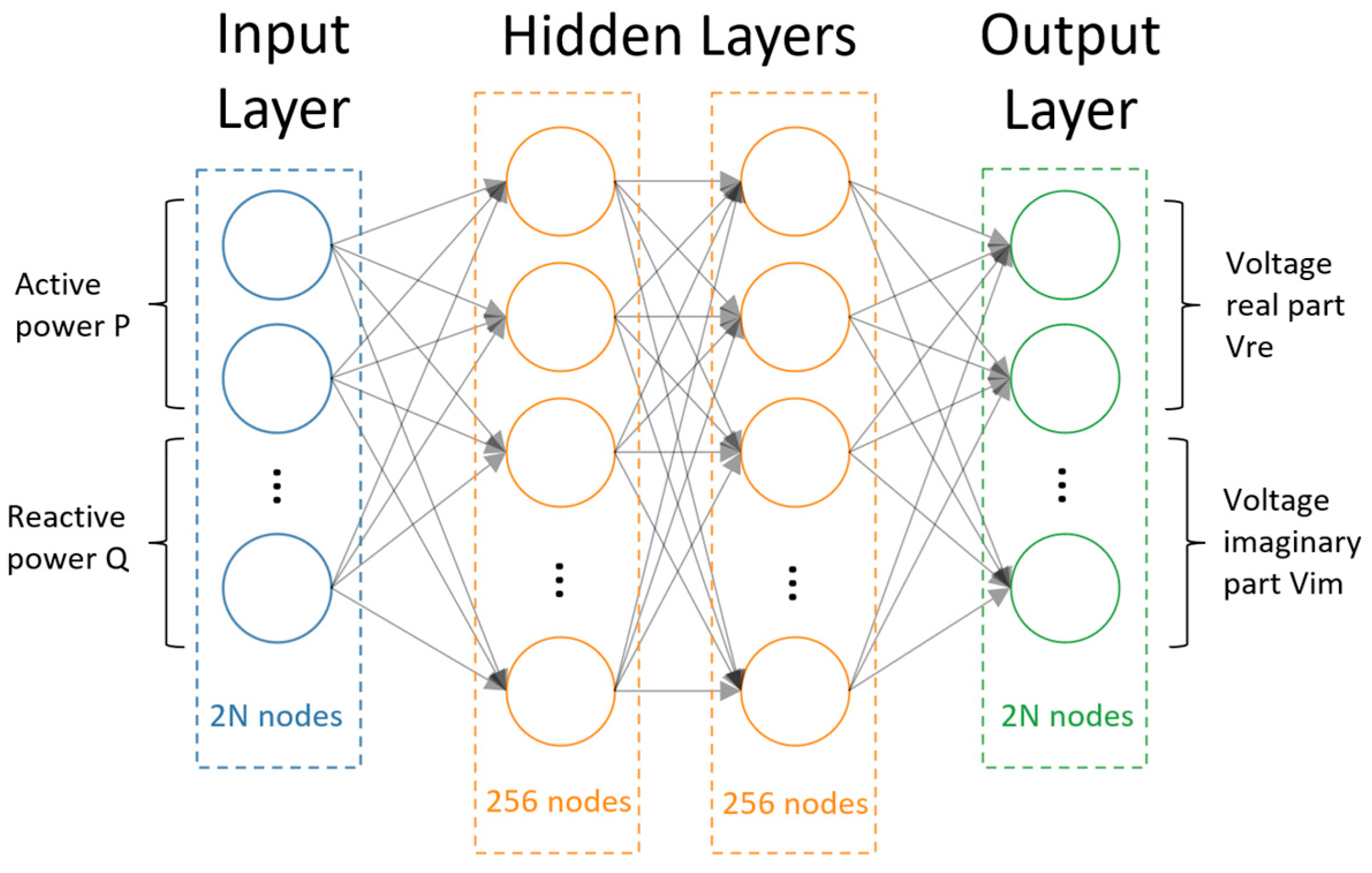
The proposed Physics-Informed Neural Network (PINN) architecture for distribution system state estimation is designed to predict the complex bus voltages—comprising both magnitudes and angles—based on complex power injections at each bus. Although the physical quantities involved are complex-valued, the network operates entirely on real-valued tensors by decomposing all complex inputs and outputs into their real and imaginary parts. The architecture comprises the following key components, schematically presented in Figure 1:

• Input Layer: The input to the network consists of the complex power injections $S = P + jQ$ at each bus. These are decomposed into their real and imaginary parts and concatenated to form a real-valued input vector of size $2N$, where $N$ is the number of buses in the network.
• Hidden Layers: The core of the model consists of two fully connected hidden layers, each with 256 neurons and hyperbolic tangent (Tanh) activation functions. This configuration was selected based on preliminary hyperparameter tuning, which showed that 256 neurons per layer provided a favorable trade-off between model capacity and computational efficiency. The use of Tanh activations further supports the network’s ability to capture complex nonlinear mappings while ensuring smooth gradients for optimization.
• Output Layer: The network outputs a real-valued vector of size $2N$, which is interpreted as the real and imaginary parts of the estimated complex bus voltages. Specifically, the first $N$ entries correspond to $Re\left(V\right)$ and the next $N$ entries to $Im\left(V\right)$.

By representing complex variables as concatenated real-valued vectors, this architecture enables efficient training using standard real-valued deep learning frameworks while preserving the underlying structure of complex-valued power system quantities.

The key innovation in the PINN approach is the physics-informed loss function that combines data-fitting terms with physics-based constraints. The total loss is formulated as:

$$L_{total}=L_{voltage}+\lambda L_{current}$$

(3)

where $L_{voltage}$ measures how well the estimated voltages match the available measurements, $L_{current}$ encodes the physics constraints by evaluating consistency with current injections, and $\lambda$ is a regularization parameter (or weighting coefficient) that controls the trade-off between data fidelity and physics consistency. This approach falls under the broader category of physics-based regularization [19,25], where physical knowledge is integrated as a soft constraint into the learning process. It enables the neural network to generalize better by leveraging both measurements and domain knowledge, making it particularly effective in power system applications.

The voltage loss $L_{voltage}$ quantifies the discrepancy between estimated and measured voltage states using the Mean Squared Error (MSE):

$$L_{voltage}={\displaystyle \frac{1}{m}}\sum _{i = 1}^m{⌈V_i-\widehat{V_i}⌉}^2$$

(4)

where m is the number of measurements, $V_i$ is the measured voltage, and $\widehat{V_i}$ is the predicted voltage phasor at node $i$.

The physics-based current loss $L_{current}$ enforces adherence to power flow equations by ensuring that the predicted voltages lead to consistent current injections. More specifically, the predicted voltages based on the power injections are utilized to calculate the currents that emerge using the equation:

$$\widehat{\mathbf{I}}=\mathbf{Y}·\widehat{\mathbf{V}}$$

(5)

where $\widehat{\mathbf{I}}$ is the estimated current injection vector and $\mathbf{Y}$ is the network admittance matrix encapsulating the specific topology and impedance of each node. These estimated currents are then compared against the true current injections obtained from the simulation dataset using Mean Absolute Error (MAE):

$$L_{current}={\displaystyle \frac{1}{m}}\sum _{i = 1}^m⌈I_i-\widehat{I_i}⌉$$

(6)

All computations are performed in the complex domain, and vectorized operations are used to ensure computational efficiency. Due to the numerical sensitivity of power system calculations and the wide dynamic range of involved quantities, double-precision arithmetic is often required to ensure stability and accuracy, especially when working in the complex domain.

In this work, the weighting coefficient $\lambda$ that balances the data-driven voltage loss and the physics-based current loss is treated as a constant, manually tuned through trial-and-error to achieve stable training and optimal performance across test cases. While this fixed weighting strategy is simple and effective, future extensions could adopt dynamic or adaptive weighting schemes that adjust $\lambda$ during training. Such approaches, including curriculum learning, uncertainty-aware weighting, or bilevel optimization, have been shown in other domains to improve convergence and robustness by gradually emphasizing the physics term as the model becomes more accurate. This flexibility could enhance the PINN’s adaptability to different network sizes, observability conditions, and noise levels.

2.3. Training

Training the PINN for distribution system state estimation involves a structured pipeline consisting of data preprocessing, optimization, and evaluation. The full dataset is first randomly partitioned into training and test subsets, typically using an 80/20 split. Preprocessing steps, including normalization, are applied only to the training set to avoid data leakage and ensure fair evaluation of generalization.

All complex-valued inputs and targets are normalized to stabilize training and prevent numerical instabilities. This is especially important to mitigate exploding values, which can occur during the initial epochs due to inaccurate current estimates derived from poorly initialized voltage states. A robust normalization technique is applied separately to the real and imaginary parts of the data. For a given complex tensor $x=x_{re }+ j{x}_{im}$, the normalized components are computed as:

$$x_{re,norm}={\displaystyle \frac{x_{re}-{\mu }_{re}}{{\sigma }_{re}}},\hspace{1em}\hspace{1em}{x}_{im,norm}={\displaystyle \frac{x_{im}-{\mu }_{im}}{{\sigma }_{im}}}$$

(7)

where ${\mu }_{re}, {\mu }_{im}$ are the means, and ${\sigma }_{re}, {\sigma }_{im}$ are the standard deviations of the real and imaginary parts, respectively, computed across the batch.

Although this normalization is based on the standard z-score approach, it incorporates several important modifications to enhance robustness for complex-valued power system data:

• The standard deviations are clamped from below using a small multiple of the corresponding mean absolute value to avoid division by near-zero values that could lead to numerical instability.
• The resulting normalized values are clipped to a predefined range (e.g., [−10, 10]) to limit the influence of outliers and prevent gradient explosions.
• The process is applied independently to each component of the complex values, which is not typical in standard real-valued z-score normalization.

These enhancements make the method more reliable for use in physics-informed training where both scale sensitivity and complex-valued operations are involved.

The network parameters are optimized using the Adam algorithm [26], a first-order gradient-based optimizer. The learning rate is adjusted dynamically using a “reduce on plateau” scheduler, which reduces the learning rate when the validation loss ceases to improve. Specifically, if the loss does not decrease for a defined number of epochs (patience), the learning rate $\eta$ is updated according to:

$${\eta }_{new} = {\eta }_{old} \times factor$$

(8)

where $factor$ is a multiplicative constant (e.g., 0.5). This adaptive strategy allows the model to make large updates when learning is active and finer updates as it approaches convergence. To further enhance stability, gradient norms are clipped to a maximum value of 1.0 during backpropagation.

Key hyperparameters—including the learning rate, batch size, number of training epochs, and the regularization factor $\lambda$ between data and physics losses—are manually tuned to achieve a good balance between data fitting and physical consistency. During training, the model state with the lowest total validation loss is checkpointed and used for final evaluation.

2.4. Case Studies and Simulations

To evaluate the performance of the proposed PINN-based state estimation approach, a series of simulation studies were conducted on standard IEEE test feeders [27], spanning a wide range of network sizes and levels of complexity. The selected systems include the IEEE 13-bus, 34-bus, 37-bus, and 123-bus feeders. These networks represent increasingly large and unbalanced low-voltage and medium-voltage distribution systems, offering a robust benchmark for assessing the accuracy, scalability, and robustness of the proposed method.

For each test system, synthetic datasets were generated using OpenDSS simulations accessed through its Python interface (OpenDSSDirect 0.9.1). A custom simulation script was developed to introduce realistic variability by randomly perturbing the real and reactive power demands of all loads. Specifically, uniformly distributed scaling factors in the range [0.8, 1.2] were applied independently to $P$ and $Q$ values, emulating diverse operating conditions. For each scenario, the resulting complex nodal voltages $\mathbf{V}$, current injections $\mathbf{I}$, and apparent power injections $\mathbf{S}$ were extracted and stored. This process was repeated for 10,000 randomized load configurations per network, yielding rich datasets suitable for supervised training and evaluation of the PINN. The complex nodal admittance matrix $\mathbf{Y}$ was also extracted once at the beginning of the simulation process and reused for all scenarios.

To thoroughly assess the robustness and generalization ability of the model, the case studies cover the following scenarios:

• Normal Operation: Base-case operation with nominal loading and full measurement availability, used to benchmark accuracy under ideal conditions.
• Limited Observability: Scenarios with sparse sensor deployment, where voltage and power measurements are only available at a subset of buses, testing the model’s extrapolation capability.

These comprehensive simulations provide insight into the behavior of the PINN across practical operating conditions and potential real-world challenges encountered in distribution system monitoring.

2.5. Performance Metrics

To assess the performance of the selected models, we employ widely used evaluation metrics that capture different aspects of accuracy and reliability. These metrics evaluate both absolute and relative deviations between the estimated and true values:

$$MAE={\displaystyle \frac{1}{n}}\sum _{i = 1}^n\left|y_i-\widehat{y_i}\right|$$

(9)

$$RMSE=\sqrt{{\displaystyle \frac{1}{n}}\sum _{i = 1}^n{\left(y_i-\widehat{y_i}\right)}^2}$$

(10)

where $y_i$ and $\widehat{y_i}$ denote the true and predicted values, respectively, and $n$ is the number of test samples. MAE corresponds to the ${\mathcal{l}}_1$-norm of the error vector, providing a linear penalty for deviations. RMSE corresponds to the ${\mathcal{l}}_2$-norm, emphasizing larger errors due to the squaring operation [28]. Together, these metrics enable robust quantitative comparison of model performance across scenarios and test systems.

3. Results and Discussion

To evaluate the performance of the proposed PINN-based state estimation algorithm, two scenarios are considered:

• Baseline—a model trained without incorporating physical constraints (no current loss);
• PINN—a model trained with the current loss term to enforce physical consistency.

To ensure consistency across experiments, the same set of hyperparameters was used for training all models.

Table 1. Summary of training hyperparameters used for all models.

Hyperparameter		Value
Optimizer		Adam
Activation Function		Tanh
Hidden Layers		2
Hidden Units Per Layer		256
Timestamps		10,000
Scheduler	Learning Rate (Initial)	0.01
	Patience	50 epochs
	Factor	0.5
Epochs		2000
Train–Test Split		0.8–0.2
λ Loss Weights		~0.001

summarizes the key training configurations applied in this work. The models were trained using the Adam optimizer, which offers adaptive learning rate adjustment and typically ensures faster convergence for deep networks. A modest architecture was employed, consisting of two hidden layers with 256 units each and tanh activation functions, balancing model expressiveness and overfitting risk. The total dataset comprised 10,000 time-indexed samples, split into training and testing subsets using an 80–20 ratio. The learning rate was initially set to 0.01 and adjusted dynamically during training through a scheduler with a patience of 50 epochs and a reduction factor of 0.5 when no improvement was observed. Training lasted up to 2000 epochs, although early stopping was effectively managed through the scheduler. Finally, the weights of the composite loss terms—associated with voltage and current equations—were set empirically, with λ values on the order of 0.001 to balance physical consistency and prediction accuracy.

Initially, both models are evaluated under noise-free conditions. They are trained using identical hyperparameters, and the resulting performance on the test set is presented in

Table 2. Test set results.

	Baseline		PINN		Improvement (%)
	MAE		MAE		MAE
	Voltage	Current	Voltage	Current	Voltage	Current
ΙΕΕΕ13	0.28	24.04	0.18	0.62	37.28	97.43
ΙΕΕΕ34	2.03	17.45	1.73	3.1	14.82	82.27
ΙΕΕΕ37	0.85	7.34	0.29	0.43	66.2	94.07
ΙΕΕΕ123	0.28	5.46	0.21	0.45	22.92	91.72
	RMSE		RMSE		RMSE
	Voltage	Current	Voltage	Current	Voltage	Current
ΙΕΕΕ13	0.44	52.6	0.28	1.12	37.13	97.87
ΙΕΕΕ34	2.87	52.92	2.47	7.7	13.77	85.45
ΙΕΕΕ37	1.06	26.45	0.39	0.56	63.67	97.88
ΙΕΕΕ123	0.37	21.8	0.28	0.64	22.44	97.07

. As shown, the PINN significantly outperforms the baseline by leveraging the physics-based constraint, leading to substantially lower current estimation errors while maintaining or improving voltage accuracy. This demonstrates that, under the same training conditions, the PINN is capable of learning the underlying physical behavior of the network and generating voltage estimates that yield highly accurate current predictions.

In addition to the test set performance, the training behavior of the models provides further insights. Figure 2 illustrates the training metrics over the first 100 epochs for each network. It is evident that the PINN exhibits significantly faster convergence compared to the baseline model. In all cases, the PINN rapidly reduces both voltage and current errors within the first few epochs, indicating more efficient learning of the system’s underlying physics. In contrast, the baseline model demonstrates a slower, more gradual reduction in error, requiring many more epochs to approach comparable levels of accuracy. This accelerated convergence of the PINN underlines the benefit of embedding domain knowledge directly into the learning process. By enforcing physical constraints during training, the model not only learns faster but also generalizes more robustly. Moreover, this advantage becomes increasingly pronounced as the network size scales up. Observing the progression from IEEE13 to IEEE123, the gap between the baseline and PINN performance—particularly in terms of current loss (red curves)—widens substantially. The expanding area between the solid and dashed red lines signifies the growing benefit of physics integration in larger, more complex systems, where conventional data-driven approaches struggle to efficiently capture the nonlinear interactions inherent in distribution networks.

To qualitatively assess the model’s performance, we examine a randomly selected timestamp from the test set corresponding to the IEEE 13-bus system—the smallest test case considered.

Table 3. Results from IEEE13 for a random timestamp. Cells with poor ANN predictions are highlighted for clarity.

Bus	Voltage Magnitude		Voltage Angle (°)		Current Magnitude		Current Angle (°)
	Actual	Pred.	Actual	Pred.	Actual	Pred.	Actual	Pred.
SOURCEBUS.1	66,395	66,395	29.99	29.99	16.01	13.77	2.91	5.36
SOURCEBUS.2	66,396	66,396	−90.01	−90.01	18.23	18.07	−105.82	−106.19
SOURCEBUS.3	66,393	66,393	149.99	149.99	20.03	18.26	123.36	118.33
650.1	2402	2402	−0.01	−0.01	0.00	10.42	0.00	−7.95
650.2	2402	2402	−120.01	−120.01	0.00	16.40	−123.69	169.79
650.3	2402	2402	119.99	119.99	0.00	27.15	−122.01	−161.62
RG60.1	2551	2551	−0.01	−0.01	0.00	64.43	−78.12	179.55
RG60.2	2522	2522	−120.01	−120.01	0.00	4.62	−29.39	−47.97
RG60.3	2566	2567	119.98	119.98	0.00	16.11	135.27	61.51
633.1	2466	2466	−2.34	−2.34	0.00	0.83	−87.61	178.95
633.2	2501	2501	−121.57	−121.57	0.00	0.47	0.00	95.57
633.3	2449	2449	117.80	117.80	0.00	0.28	0.00	−90.84
634.1	278	279	−2.85	−2.84	618.29	613.84	138.59	138.72
634.2	284	284	−121.97	−121.97	511.60	512.50	18.87	18.85
634.3	278	278	117.28	117.28	516.61	515.37	−95.81	−95.51
675.1	2400	2400	−5.21	−5.20	197.29	197.28	154.11	153.39
675.2	2543	2543	−122.15	−122.14	34.56	34.40	15.33	14.10
675.3	2363	2364	116.15	116.16	173.16	173.51	−101.59	−101.83
611.3	2364	2365	115.90	115.90	62.92	62.19	−85.62	−85.59
632.1	2472	2472	−2.31	−2.30	0.00	1.22	90.00	20.20
632.2	2506	2506	−121.53	−121.53	0.00	2.08	−153.43	−98.98
632.3	2455	2455	117.82	117.82	0.00	1.13	−101.31	82.33
670.1	2453	2453	−3.16	−3.16	8.91	8.93	144.83	148.14
670.2	2513	2514	−121.69	−121.69	36.60	37.72	24.81	26.42
670.3	2424	2424	117.19	117.19	52.56	52.94	−93.79	−93.99
671.1	2414	2414	−4.95	−4.94	150.08	160.71	151.18	143.44
671.2	2537	2537	−121.99	−121.98	150.08	126.94	31.21	39.13
671.3	2370	2371	116.13	116.13	150.14	203.73	−88.81	−87.49
680.1	2414	2415	−4.95	−4.94	0.00	0.50	104.04	−80.56
680.2	2537	2537	−121.99	−121.98	0.00	0.08	−36.87	−67.06
680.3	2370	2371	116.13	116.14	0.00	0.67	0.00	89.30
645.3	2450	2450	117.86	117.86	0.00	0.91	0.00	−130.72
645.2	2485	2485	−121.70	−121.70	75.67	76.26	22.66	23.06
646.3	2445	2445	117.90	117.90	64.04	63.29	−122.26	−122.20
646.2	2481	2481	−121.78	−121.77	64.04	63.31	57.74	57.81
692.1	2413	2414	−4.95	−4.95	46.16	59.28	105.75	160.54
692.2	2537	2537	−121.99	−121.99	0.00	28.87	90.00	−3.53
692.3	2370	2370	116.13	116.14	46.16	11.77	−74.25	44.47
684.1	2408	2409	−4.97	−4.96	0.00	0.37	−135.00	−16.60
684.3	2367	2368	116.04	116.04	0.00	0.70	180.00	149.88
652.1	2394	2395	−4.91	−4.90	66.88	67.02	143.55	143.79

reports the actual and predicted values of voltage magnitude, voltage angle, current magnitude, and current angle for each bus. As observed, the model demonstrates excellent accuracy in estimating voltage magnitudes and angles across all buses. In terms of current estimation, the performance remains satisfactory, though some deviations are observed—primarily in buses where the actual current injections are zero. This is expected, as minor numerical deviations can yield large relative or angular errors when current magnitudes are near zero, due to the amplification of small differences in both magnitude and phase when dividing or taking angles of near-zero complex numbers. However, these errors are of limited practical significance, as the corresponding current injections are negligible in absolute terms and have minimal impact on the overall system behavior. This issue can be mitigated by explicitly incorporating prior knowledge about load and zero-injection buses, e.g., via masking or regularization.

To evaluate the robustness of the models under noisy input conditions, a new dataset was generated consisting of 1000 simulation points for each test network. Gaussian noise was then added to the input power injections at each node to simulate measurement uncertainty. The results, summarized in

Table 4. Performance metrics under noisy data input.

Noise Level (%)	Network	Baseline		PINN		Improvement (%)
		MAE		MAE		MAE
		V	I	V	I	V	I
0	IEEE13	0.26	23.44	0.17	0.60	35.13	97.43
	ΙΕΕΕ34	1.30	16.78	1.18	2.93	9.83	82.56
	ΙΕΕΕ37	0.78	7.27	0.22	0.42	72.27	94.22
	ΙΕΕΕ123	0.14	5.32	0.13	0.44	7.05	91.82
1	IEEE13	1.06	38.27	1.23	2.03	−16.04	94.70
	ΙΕΕΕ34	9.44	20.36	9.95	3.84	−5.40	81.14
	ΙΕΕΕ37	1.32	7.96	1.22	0.70	7.58	91.21
	ΙΕΕΕ123	0.74	5.45	0.79	0.48	−6.76	91.19
5	IEEE13	4.93	144.92	5.88	9.43	−19.27	93.49
	ΙΕΕΕ34	43.24	58.34	46.07	12.48	−6.54	78.61
	ΙΕΕΕ37	5.10	17.14	5.80	2.72	−13.73	84.13
	ΙΕΕΕ123	3.49	7.72	3.74	0.98	−7.16	87.31
		RMSE		RMSE		RMSE
		V	I	V	I	V	I
0	IEEE13	0.39	50.94	0.25	1.08	35.63	97.89
	ΙΕΕΕ34	1.90	50.94	1.70	7.32	10.14	85.64
	ΙΕΕΕ37	0.97	26.26	0.28	0.54	70.87	97.95
	ΙΕΕΕ123	0.20	21.09	0.17	0.62	14.52	97.08
1	IEEE13	1.47	80.58	1.73	3.32	−17.69	95.88
	ΙΕΕΕ34	12.44	60.80	13.19	8.86	−6.03	85.43
	ΙΕΕΕ37	1.58	28.36	1.44	0.86	8.86	96.97
	ΙΕΕΕ123	0.92	21.57	0.98	0.69	−6.52	96.80
5	IEEE13	6.87	306.76	8.20	15.48	−19.36	94.95
	ΙΕΕΕ34	57.09	173.26	61.25	26.98	−7.29	84.43
	ΙΕΕΕ37	6.08	59.65	6.87	3.35	−12.99	94.38
	ΙΕΕΕ123	4.33	29.98	4.67	1.60	−7.85	94.66

, demonstrate that the PINN consistently outperforms the baseline model across all networks and noise levels, particularly in terms of current estimation accuracy. Even as noise increases, the PINN maintains relatively low error metrics and high improvement percentages, highlighting its ability to learn physically consistent representations that generalize well under data perturbations. For instance, in the IEEE37 network under 5% input noise, the PINN reduces the current RMSE by over 94% (from 59.65 to 3.35) compared to the baseline, while the voltage RMSE shows a minor increase of about 13% (from 6.08 to 6.87). In contrast, the baseline model exhibits a steep degradation in performance, especially for larger networks and higher noise levels. These findings underline the inherent advantage of physics-informed training in ensuring model reliability under realistic, imperfect conditions.

A similar benchmarking procedure was conducted to evaluate the performance of the models under conditions of partial observability, simulating scenarios with missing measurements. To achieve this, a random subset of the input data (i.e., power injections) was masked, corresponding to 10% and 20% dropout rates, respectively. This emulates the practical challenge of incomplete or faulty metering in distribution networks. The results, presented in

Table 5. Performance metrics under masked out input.

Drop Out (%)	Network	Baseline		PINN		Improvement (%)
		MAE		MAE		MAE
		V	I	V	I	V	I
0	IEEE13	0.26	23.44	0.17	0.60	35.13	97.43
	ΙΕΕΕ34	1.30	16.78	1.18	2.93	9.83	82.56
	ΙΕΕΕ37	0.78	7.27	0.22	0.42	72.27	94.22
	ΙΕΕΕ123	0.14	5.32	0.13	0.44	7.05	91.82
10	IEEE13	17.14	370.93	20.25	29.11	−18.13	92.15
	ΙΕΕΕ34	113.53	185.43	112.42	52.19	0.98	71.85
	ΙΕΕΕ37	20.84	45.31	22.17	8.38	−6.34	81.50
	ΙΕΕΕ123	9.65	20.70	9.53	2.79	1.26	86.50
20	IEEE13	22.49	467.47	28.03	42.08	−24.67	91.00
	ΙΕΕΕ34	143.65	228.49	139.73	65.94	2.73	71.14
	ΙΕΕΕ37	30.65	52.01	33.07	9.69	−7.87	81.36
	ΙΕΕΕ123	12.27	28.25	12.38	3.85	−0.92	86.36
		RMSE		RMSE		RMSE
		V	I	V	I	V	I
0	IEEE13	0.39	50.94	0.25	1.08	35.63	97.89
	ΙΕΕΕ34	1.90	50.94	1.70	7.32	10.14	85.64
	ΙΕΕΕ37	0.97	26.26	0.28	0.54	70.87	97.95
	ΙΕΕΕ123	0.20	21.09	0.17	0.62	14.52	97.08
10	IEEE13	26.52	858.17	31.53	60.24	−18.88	92.98
	ΙΕΕΕ34	160.84	562.22	157.61	141.12	2.01	74.90
	ΙΕΕΕ37	25.63	154.60	27.25	10.33	−6.33	93.32
	ΙΕΕΕ123	12.35	81.65	12.47	4.97	−1.01	93.92
20	IEEE13	32.06	984.24	40.42	76.33	−26.08	92.24
	ΙΕΕΕ34	196.07	668.34	189.65	164.34	3.27	75.41
	ΙΕΕΕ37	34.88	179.37	37.98	11.84	−8.89	93.40
	ΙΕΕΕ123	15.25	111.74	15.55	6.65	−1.99	94.05

, confirm that the PINN retains a significant advantage over the baseline model, particularly in current estimation. Even as the proportion of missing inputs increases, the PINN maintains relatively low MAE and RMSE values, suggesting that its ability to incorporate physical constraints enables more reliable extrapolation under sparse data conditions. For instance, in the IEEE123 network with 20% input dropout, the PINN achieves a 94.05% reduction in current RMSE compared to the baseline. In contrast, the baseline model exhibits sharp increases in both voltage and current errors, especially in larger networks. Although some performance deterioration is observed in certain cases, the PINN consistently yields better overall state estimates than the baseline. These results demonstrate the superior robustness and generalization capability of the PINN under reduced observability—a critical feature for real-world deployment where sensor coverage is often limited.

The presented results confirm the effectiveness of the PINN approach across a range of distribution network configurations and operational scenarios. Compared to the baseline model, the PINN achieves consistently significantly lower voltage and current estimation errors across all test feeders. In noise-free conditions, the proposed model reduces current MAE by up to 97.4% and voltage RMSE by up to 63.7%, demonstrating strong fidelity to the underlying power system behavior. Under noisy conditions (e.g., 5% perturbation), the PINN maintains robust performance, achieving over 95% improvement in current RMSE for the IEEE 37-bus system. Similarly, in scenarios with partial observability—where up to 20% of the input power injections are masked—the model still yields over 93% improvement in current RMSE for large-scale feeders such as IEEE123. In some cases, the PINN exhibits slightly higher voltage errors compared to the baseline, resulting in negative improvement percentages. This is expected, as the addition of the physics-based loss prioritizes current consistency, which may occasionally compromise voltage accuracy. Nevertheless, the observed trade-off remains small and is outweighed by the substantial improvements in current estimation, which is a critical aspect of physically meaningful state estimation.

In addition to its predictive accuracy, the PINN shows faster convergence compared to the baseline model, rapidly minimizing both voltage and current loss within the first few training epochs. This accelerated learning suggests that the inclusion of physics-based constraints not only improves generalization but also guides the model more efficiently through the solution space. Moreover, the qualitative assessment on the IEEE13 system confirms the model’s ability to replicate the complex voltage and current profiles with high precision, even at buses with near-zero injections, where angle and relative errors are prone to instability.

These results collectively highlight the practical utility of the PINN framework for real-world distribution system state estimation. Its ability to generalize under uncertainty, and maintain physical consistency and scale across different network sizes suggests strong potential for deployment in modern grid monitoring and control systems—particularly in settings where measurement infrastructure is sparse or noisy.

4. Conclusions

The present study presented a comprehensive framework for applying PINNs to state estimation in unbalanced distribution power systems. By embedding physical constraints—specifically current consistency derived from power flow equations—directly into the training process, the proposed method effectively integrates the strengths of data-driven learning and physical modeling. Evaluation across four IEEE benchmark feeders (13, 34, 37, and 123 buses) demonstrates that the PINN consistently outperforms baseline neural networks trained without physical supervision. Specifically, the model achieves up to a 97.9% reduction in current RMSE and up to a 66.2% reduction in voltage MAE, while also exhibiting up to a 95% improvement under 5% noise and over a 93% improvement in current estimation under 20% input dropout, showcasing its robustness under realistic, imperfect conditions.

In addition to its accuracy, the PINN demonstrates rapid convergence—reducing both voltage and current errors significantly within the first 20 epochs—and provides fast inference during deployment through a single forward pass. These attributes make it highly suitable for real-time applications in distribution system monitoring.

Future research directions include incorporating prior knowledge about load and zero-injection buses, either through masking mechanisms or structured supervision, to further improve prediction quality in poorly observable areas. Additional enhancements may come from dynamic or adaptive loss weighting schemes, which allow the network to balance data fidelity and physics consistency during training. Another promising direction involves extending the framework to jointly estimate network topology and line impedances by treating the admittance matrix as a learnable parameter, provided that appropriate sparsity constraints and structural priors are introduced. Furthermore, future work may explore architectures that directly predict both voltages and currents, rather than reconstructing currents from voltages via physical constraints. Such formulations could leverage richer supervision signals and potentially yield further improvements in performance.

The proposed PINN approach offers a scalable, interpretable, and high-performing solution for distribution system state estimation, paving the way toward more intelligent, resilient, and data-efficient energy networks. However, it is important to note that the current study is based entirely on synthetic datasets generated through OpenDSS simulations. Although these datasets were designed to reflect realistic operational variability, the introduced noise and observability constraints do not fully capture the complexities of actual measurement noise and field conditions. As such, the conclusions regarding real-world applicability should be interpreted in the context of simulated environments. Future work will aim to validate the framework using real measurement data to further assess its practical deployment potential.