Experimental and Numerical Flow Assessment of the Main and Additional Tract of Prototype Differential Brake Valve

Abstract

The throughput of the pneumatic brake valve is a key parameter in ensuring fast and safe vehicle braking. The instantaneous value of this parameter determines the short response time of the system to an operator’s force. The scientific objective of this paper was to determine the throughput of brake valve tracts using numerical and experimental methods. These tracts are supposed to provide the tracking and acceleration function of the valve depending on the setting of the correction system. The first numerical method was based on polyhedral meshes using computational fluid dynamics (CFD) and Ansys Fluent software. The second research method—experimental tests on the author’s bench using the reservoir method—consisted of identifying throughputs based on pressure waveforms in the measurement tanks. The determined throughputs were averaged over the range of pressure differences tested and allowed the final calculation of the mass flow rate. The analysis of the obtained results showed an average discrepancy between the two research methods for both tracts, in which the flow in both directions was considered to be 9.43%, taking into account the use of a polyhedral numerical mesh ensuring high-quality results with an optimal simulation duration. The analysis of the pressure distribution inside the working chambers showed local areas of increased pressure and negative pressure resulting from the acceleration of the flow in narrow flow channels and the occurrence of the Venturi effect.

1. Introduction

Pneumatic brake systems, despite being partially replaced by hydraulic systems or combined systems, are still widely used in various branches of transport—tractors, trailers, agricultural tractors, railways, etc. [1,2,3,4]. Unlike hydraulic systems, pneumatic brake systems use an ecological working medium, which does not lead to environmental pollution in the event of a failure [5,6]. Limitations resulting from the long response time of the system to the operator’s input, related to the growing dimensions of the vehicle set, and legal and homologation requirements [7] in recent years have resulted in the end of production of new trailers equipped with a single-line brake system. Currently, only the production of dual-line systems using two independent circuits, namely supply and control [8,9], which provide noticeably better operational and functional properties and enable the proportional control of the system’s operation depending on the force applied to the brake pedal by the driver or operator, is permitted.

In the construction of pneumatic trailer braking systems, valves that activate the brakes after a pneumatic control signal appears at the connection connected to the main brake valve of the vehicle are used. The traditional relay valve, after supplying the control connection with a pneumatic signal, is switched to supply the output chamber from an additional tank located near the valve in proportion to the value of the control signal. In the event of emergency braking, such an approach can lead to the loss of vehicle stability and the creation of a hazard in land traffic. In the works of the authors of [10], the possibility of introducing a design modification was noted by using an additional control channel in a commercial pneumatic relay brake valve. Changing the direction of compressed air flow inside the valve body and connecting the chambers above and below the piston controlling the channel with an appropriately selected [11] or regulated pneumatic capacity as a function of load will enable the tracking function of the brake system to be maintained or an accelerating action to be obtained when the capacity of the control channel is too insufficient to quickly equalize the pressures in the chambers controlling the operation of the differential tract. After the accelerating action has ceased, the valve, in accordance with the assumptions, should return to proportional action depending on the force applied to the brake lever by the operator.

Each component of the pneumatic system is characterized by the occurrence of resistance to the flow of the working medium resulting from the friction of the working medium on the walls of the surfaces limiting the flow, changes in the flow direction resulting from the geometry of the element, the degree of opening and the initial and instantaneous value of the pressure difference before and after the resistance. In practice, this state causes losses and pressure drops in relation to the input values. The determination of the static flow characteristic [12,13,14,15] of the pneumatic resistance, in the case of a pneumatic brake valve, is possible using experimental methods; these are divided into the direct method, which involves measuring the mass flow rate using flow meters, as well as the indirect (tank) method, based on recording the pressure course before and after the resistance in pneumatic capacities of known-volume tanks. Using the mathematical description based on the lumped method (lumped volume method) [16,17] of the tested system with the use of numerical identification based on the developed flow model, it is possible to determine the pneumatic resistance capacity in Matlab-Simulink and finally determine the mass flow rate (MFR).

An alternative approach to determining the static flow characteristics involves the use of computational fluid dynamics (CFD) tools based on the RANS (Reynolds Average Navier-Stokes) model [18], describing the flow processes in each cell of the compressed air volume of the considered volume based on the declared numerical grid. A key aspect of using CFD tools is the declaration of the boundary conditions of the model consistent with the conditions of the actual operation of the tested pneumatic assembly and the selection of a finite element mesh discretizing the spatial model of the fluid, liquid or gas volume, ensuring high-quality results at the optimal duration of the numerical simulation. In the problem under consideration, the Ansys Fluent environment was used, which provides wide possibilities for declaring lumped volume meshes and polyhedral domains [19,20,21] based on polyhedral spatial cells after transforming the basic tetrahedral mesh. According to the literature studies and the authors’ earlier work [22], such an approach ensures the attainment of real results while maintaining the optimal duration of the simulation.

Despite the fact that a number of experimental studies have been conducted on the effectiveness of pneumatic brake systems, a lack of detailed studies on the flow characteristics of the component paths of brake valves [23,24,25] was found. This was the basis for formulating a research gap, which indicated the need for the flow characteristics of individual paths of pneumatic brake valves to be determined. Very often, in modelling using empirical models [26], the flow characteristics of brake valves are described by a rectangular characteristic, based on the minimum and maximum value. This results in discrepancies in the times required to reach the reference pressures during the validation of such models. Additionally, despite the significant development of computer techniques, their common use in the flow assessment of flow paths of brake valves was not found.

The scientific objective of this study was to determine the capacity of the main and additional supply path of a modified pneumatic brake relay valve. The achievement of this goal was realized in experimental and model conditions. The experimental determination of the capacity of both paths depending on the degree of opening will allow the determination of the static characteristics of both paths using empirical relationships. The CFD computer simulation method based on the 3D model of the considered brake valve using the Ansys Fluent environment allows for verification, an assessment of the validity and the validation of the numerical approach to solving static problems related to pneumatic brake valves. The conclusions of the above analyses constitute an introduction to dynamic tests and valve configuration in order to obtain the dual-range operation assumed by the authors.

The rest of the article is as follows. Section 2 presents the object of analysis with a detailed description of both supply tracts. The basics of the adopted experimental and numerical research methodology in the CFD Ansys Fluent environment are described. Section 3 presents the results obtained in the experimental and numerical research, taking into account both directions of compressed air flow during braking and debraking. Section 4 contains an analysis and discussion of the obtained results. Section 5 contains conclusions, and Section 6 presents further directions for research.

2. Materials and Methods

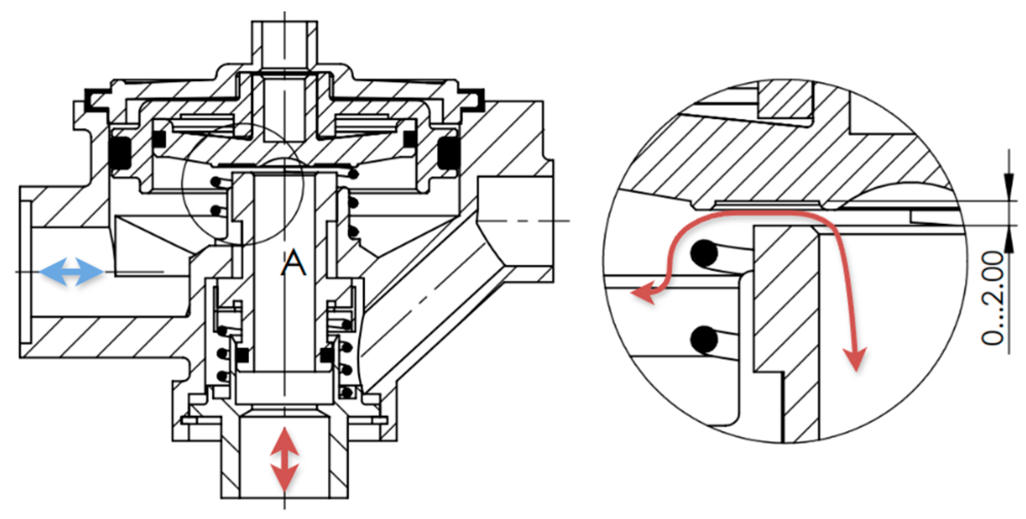
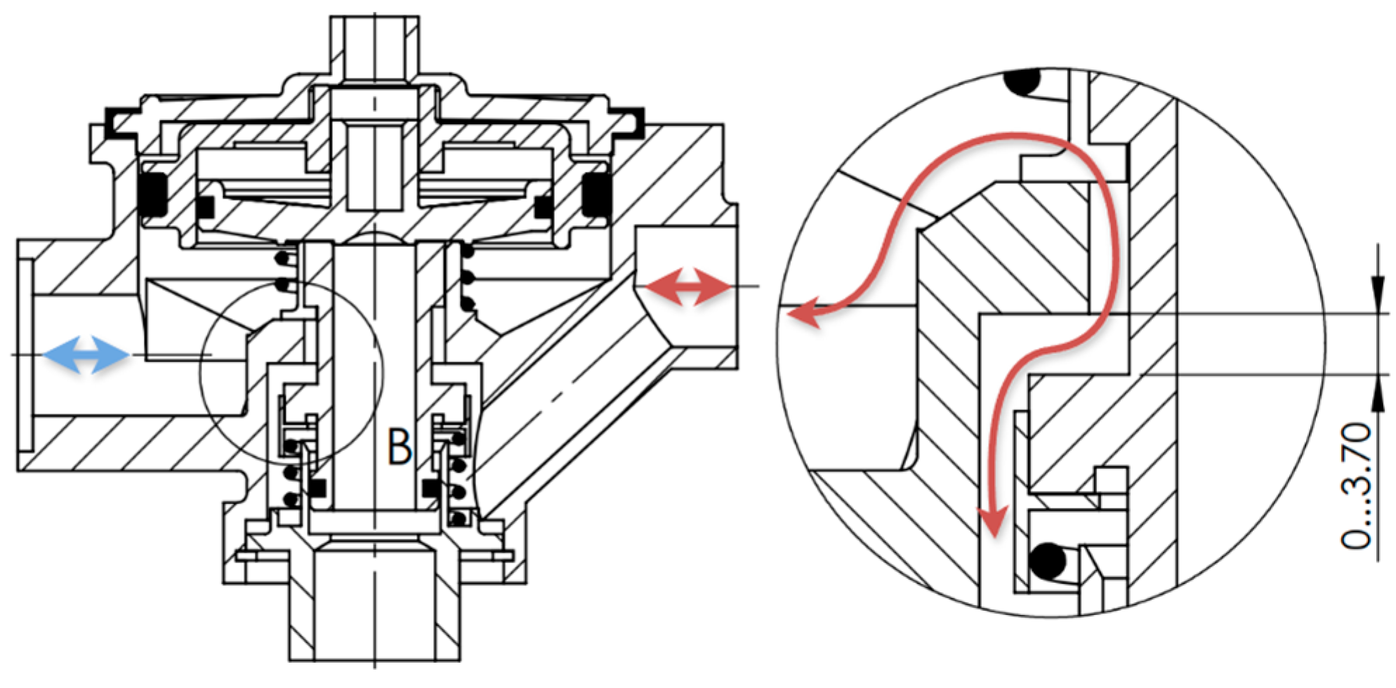
2.1. Object of Analysis

The determination of the nozzle capacity of the differential tract using the experimental and numerical methods was undertaken in the authors’ earlier work. The operation of the differential tract determines the operation of the supply section under consideration by controlling its opening degree. Conducting static tests leading to the determination of the capacity of both supply sections of the prototype pneumatic differential valve required the use of only a part of the valve and is the last stage of preparatory work for further dynamic tests. In the case of the numerical approach, it was necessary to introduce minor modifications to the 3D model, while the experimental tests required the use of additional assembly elements enabling the precise control of the degree of opening of both valve sections, which is by default achieved by moving the piston assembly and the differential section guide [27].

In order to prepare the valve for experimental tests, it was necessary to introduce a few modifications in accordance with Figure 1. A rivet nut 14 and an adjustment screw 15 were placed in the guiding element 12, the degree of which, together with the additional spring 17 supporting the control piston 8, enabled the precise positioning of the piston inside the valve body 7 to be determined. A digital dial gauge placed in the axis of the adjustment screw using a mounting element made on a 3D printer was used to assess the degree of adjustment of the control piston (Figure 2).

The main supply tract regulated by opening the gap between the bushing 3 and the control piston 8 enabled the valve to maintain its tracking function in accordance with the diagram and flow direction shown in Figure 3.

In the event of a differential action, the displacement of the control unit (replaced by a screw for the purposes of the experimental tests) is large enough to close the main supply tract and open the flow between the additional compressed air tank connection and the valve output connection after overcoming the friction and the force contained in the spring 5 supporting the control bushing 3 via the spring base 4 in accordance with Figure 4.

The equalization of the forces acting on the surfaces of the control piston of the differential tract and the force generated by the spring 5 supporting the adjustment bushing causes the entire control unit to move upwards, closing the supply from the additional connector and returning to the proportional supply conditioned by the force exerted on the brake lever by the operator.

The lack of studies related to determining the static characteristics of a differential valve with a two-range operation by the experimental method forced the development of a system for regulating the valve opening degree. Therefore, during the tests, only the part of the valve responsible for controlling the supply was used, and the actuating piston assembly with the guide was replaced with a threaded drive. The opening degree of individual supply sections was regulated with a screw by setting the zero position and observing the displacement using a digital dial gauge. The opening degree of the supply buses was regulated every 0.25 mm in the range of (0.25–2.00) mm for the main supply tract and in the range of (0.25–3.70) mm for the additional tract (the accuracy of the dial gauge was—0.01 mm). Analogous boundary conditions were adopted in the 3D model developed in SolidWorks 2024, where the opening degree was regulated by editing the constraints between the cooperating planes of the model, which were then exported to the STEP file format. The models prepared in this way were loaded into the Ansys Fluent 2024 software, and the details are described in Section 2.3.

2.2. Experimental Research

Experimental tests of both supply tracts were carried out on the developed test stand (Figure 5) operating in accordance with the design assumptions of the tank method, which allows for determining, among others, the static flow characteristics of the tested pneumatic resistance. The possibility of using this approach was confirmed in previous publications by the authors mentioned in previous sections, as well as in other literature [28,29], drawing attention to its high effectiveness in determining the flow parameters of compressed air, as well as other gases. The measurement principle involves recording the pressure courses in two tanks of known volume, between which a solenoid valve is mounted to start the measurement, and directly behind it is the tested brake valve 8 (Figure 5).

The recording of pressure courses in the measuring tanks, the algorithm controlling the sequence of solenoid valves and the acquisition of results with a sampling time of 3 ms were implemented using the Python 3.11 language and the additional PyQT5 graphic library using the Raspberry Pi 3 microcomputer Raspberry Pi Foundation (Cambridge, UK). The current readings can be viewed and the station can be operated using a dedicated touch screen. The practical implementation of the station is shown in Figure 6. During the tests, a counter was declared, which automatically enabled the measurement to be repeated five times.

The measurement sequence of one measurement is as follows:

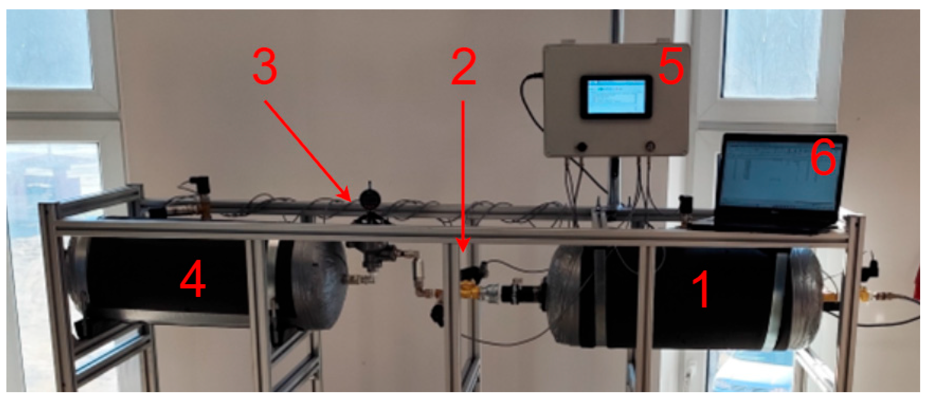
• Open the solenoid valve 3 supplying the measuring system from the compressed air preparation station and fill the supply tank 6 to the working pressure;
• Close the supply solenoid valve 3, stabilize the pressure in the supply tank 6 and start pressure recording to a *.csv file with the declared sampling time;
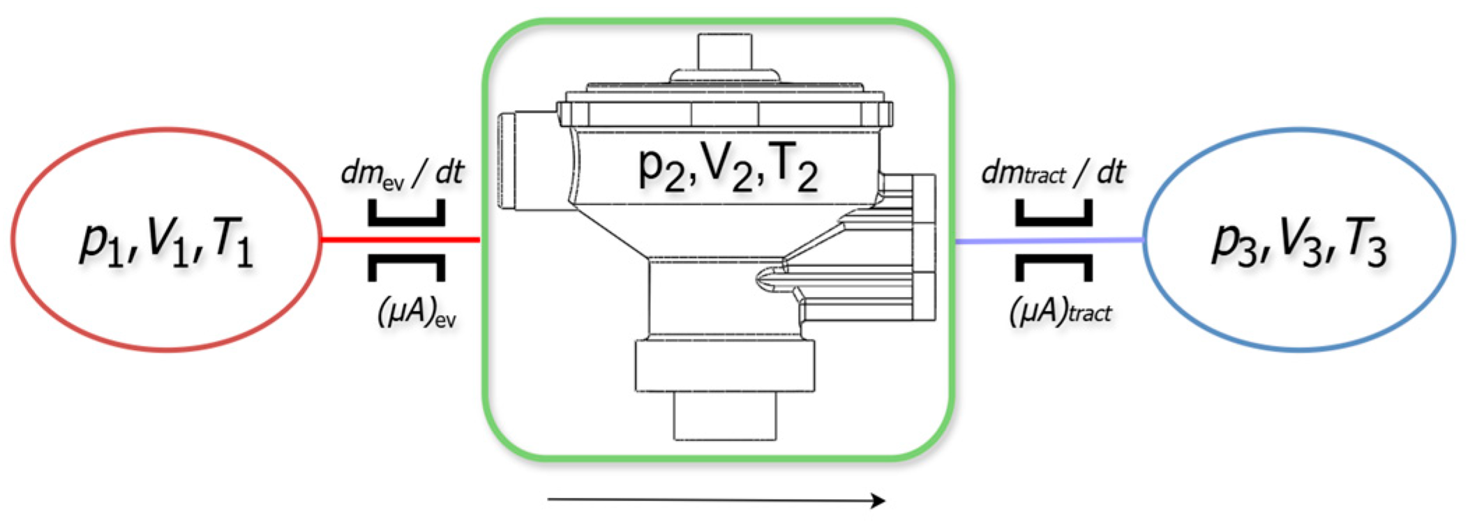
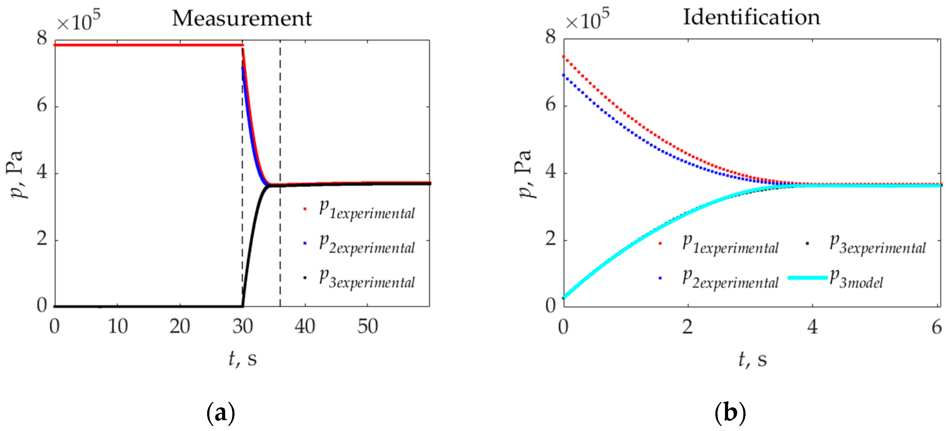
• Open the measuring solenoid valve 7 and flow of compressed air from the supply tank 6 to the measuring tank 9 through the brake valve. The flow is caused by the pressure gradient in both tanks;
• After equalizing the pressure in both tanks, end the recording, close the measuring solenoid valve 7, save the *.csv file, open the release solenoid valves 5 and 10, enabling the pressure in both tanks to equalize to the atmospheric pressure, and close it to ensure the re-sealing of the measuring system;
• Ending a measurement sequence after reaching the specified repetition counter causes the program to terminate or loop if the required number of repetitions has not been reached.

The measurement file in *.csv format, in accordance with Figure 5 and the adopted methodology, contains input data for the MATLAB environment, which, after implementing the mathematical description of the station based on the lumped method [30], enables the identification of flow parameters, in particular the effective flow field (μA)_tract, the value of which is mainly dependent on the geometry of the compressed air flow channels. Determining the (μA)_tract value from the pressure curves in both tanks allows the determination of the mass flow rate MFR for each valve opening degree and the plotting of the static characteristics.

Based on the schematic description of the research stand (Figure 7) and the lumped method, for each concentrated volume in the considered system, a description of the mass flow of the inflowing or outflowing gas can be presented according to the basic relationship in Equation (1).

$$Q={\displaystyle \frac{dm}{dt}}={\left(\mu A\right)}_i{v}_{max}\rho {\phi \left(\sigma \right)}_{max}f(\sigma )$$

(1)

where (μA)_i—throughput of pneumatic resistance; v_max—maximum air speed; ρ—gas density (air); ${\phi \left(\sigma \right)}_{max}$–Saint-Venant–Wantzel function maximum value; f(σ)—dimensionless Myetluk–Avtushko flow function.

By adopting idealized flow conditions and a simplification excluding heat exchange with the environment during the flow (adiabatic process), it is possible to simplify Equation (1) to Equation (2) by describing the value of the adiabatic mass flow rate through the nozzle.

$$Q={\displaystyle \frac{dm}{dt}}={\displaystyle \frac{V}{\kappa RT}}{\displaystyle \frac{dp}{dt}}$$

(2)

where: $V$—volume of the node.

Figure 7 shows the assumed instantaneous values of pressure and temperature in the lumped volumes; in accordance with the lumped method, the mass balance of the component streams in each of the three lumped volumes was described using differential equations by taking into account the flow direction (in accordance with the direction of the arrow in Figure 7), as shown in Equations (3)–(5).

$${\displaystyle \frac{d{p}_1}{dt}}=-{\displaystyle \frac{\kappa RT}{V_1}}\left({\left(\mu A\right)}_{evalve}\sqrt{\kappa RT}{\displaystyle \frac{p_1}{RT}}{\phi }_{max}a{\displaystyle \frac{p_1-p_2}{a{p}_1-p_2}}\right)$$

(3)

$${\displaystyle \frac{d{p}_2}{dt}}={\displaystyle \frac{\kappa RT}{V_2}}\left({\left(\mu A\right)}_{evalve}\sqrt{\kappa RT}{\displaystyle \frac{p_1}{RT}}{\phi }_{max}a{\displaystyle \frac{p_1-p_2}{a{p}_1-p_2}}{-\left(\mu A\right)}_{tract}\sqrt{\kappa RT}{\displaystyle \frac{p_2}{RT}}{\phi }_{max}a{\displaystyle \frac{p_2-p_3}{a{p}_2-p_3}}\right)$$

(4)

$${\displaystyle \frac{d{p}_3}{dt}}={\displaystyle \frac{\kappa RT}{V_3}}\left({\left(\mu A\right)}_{tract}\sqrt{\kappa RT}{\displaystyle \frac{p_2}{RT}}{\phi }_{max}a{\displaystyle \frac{p_2-p_3}{a{p}_2-p_3}}\right)$$

(5)

where κ—adiabatic exponent; (μA)_evalve—electrovalve throughput; (μA)_tract—throughput of brake valve tract; R—gas constant (air); φ_max—Saint-Venant–Wantzel theoretical function maximum value; a = 1.13—Myetluk–Avtushko coefficient value.

The use of the solenoid valve controlling the start and end of the measurement (7 in Figure 5) with the capacity (μA)_evalve (Figure 7), which is not the subject of the research, resulted in us only taking into account the pressure courses recorded using the transducer placed behind the start solenoid valve p₂ and the measuring tank p₃ to identify the capacity of the valve (μA)_tract. In connection with the above, the search for the capacity of the tested valve tract (depending on the supply and outlet connections, and consequently the flow direction) was limited to determining the capacity (μA)_tract based on Equation (5), using the implicit trapezoidal integration method used in the numerical solution of ordinary differential equations. The implicit trapezoidal method [31] can be considered in the context of the Runge–Kutta method and the multistage linear method. The tract capacity (μA)_tract was determined using the least squares regression method in Equation (6), while the minimization of squared deviations was performed using the downhill simplex method [32,33] to find the minimum value in the multidimensional space.

$$S_{\left(residuals\right)}=\sum _{i=1}^n{(y_i-\overline{y_i})}^2=\sum _{i=1}^n{\left(p_{3experimental}-p_{3model}\right)}^2\Rightarrow minimum$$

(6)

The methodology of searching for the capacity value (μA)_tract according to Equation (6) consisted in comparing the experimental pressure curve in the measuring tank p_{3experimental} with the model curve p_3model obtained from the solution of Equation (5) in the lumped volume V₃. The assessment of the fit of both curves was made using the MAPE index.

The identification of the valve capacity required the recorded pressure time course to be limited to the stabilized flow area, where the influence of transient processes was excluded. In the course thus determined, the measurement points were normalized and the valve capacity (μA)_tract was searched for in accordance with the methodology presented above. An example of the pressure time course recorded for 0.5 mm of the main supply tract opening during the experimental tests is shown in Figure 8a, and its stabilized flow fragment subjected to capacity identification is shown in Figure 8b.

The identification of the capacity of the two supply tracts of the modified brake valve was repeated five times for each degree of opening set by the adjustment screw. The tests were repeated for the opposite direction of compressed air flow in order to determine the hysteresis of the static characteristic of the tested valve, which is an important criterion during the operation of the valve in the conditions of actual operation in the pneumatic brake system. The determined capacity values for each measurement were substituted into Equation (1), which allowed us to determine the experimental value of MFR for different degrees of opening in both supply paths, which were evaluated and compared with the results of the numerical analyses in Section 3.

2.3. Numerical Studies in ANSYS Fluent

CFD numerical calculations enabling the evaluation of flow parameters were developed based on the FVM method [34,35]. Model discretization, i.e., the extraction of the flow volume from the 3D model and its division into smaller cells of various shapes, the size of which is defined during the preparation of the numerical model mesh, makes it possible to search for the values of the working medium parameters, such as the flow velocity, pressure or temperature, in any defined cross-section of the model without the need to search for a general solution. Due to the extensive mesh generation capabilities of the Ansys Fluent environment, a tetrahedral mesh with polyhedral domains was used to search for a solution to the described problem, which in effect enabled the creation of a finite volume mesh with a polyhedral shape, highly reflecting the volume of compressed air inside the valve chambers, as well as optimizing the computation time. Polyhedral meshes are widely used in numerical simulations, constituting an optimal solution in terms of the quality of the obtained results, with a significantly shorter time necessary to obtain a solution to a given problem. The flow parameters of the stream in numerical methods are determined by numerically solving partial differential equations describing the behaviour of the velocity and pressure fields of a gas or liquid based on the principles of the conservation of momentum and mass, called the Navier–Stokes equations [36].

$${\displaystyle \frac{\partial p}{\partial t}}+\nabla \left(pv\right)=0$$

(7)

$$p{\displaystyle \frac{\partial v}{\partial t}}=-\nabla p+\rho g+\mu {\nabla }^{2}v$$

(8)

In fluid mechanics, two basic types of flow can be distinguished, namely laminar and turbulent, whereby in the considered case, the focus was on turbulent flow and the k-ε model was used with an additionally defined value of turbulence intensification I = 2% and a length L = 7 × 10⁻⁵ m. Such selected parameters in the case of a pneumatic brake valve and solving the problem using the RANS model in the authors’ earlier works enabled the attainment of highly accurate turbulent flow simulation in near-wall areas and local flow constrictions resulting from the valve geometry. The RANS model allows one to take into account the influence of local vortices caused by turbulent flow on the flow parameters, considering the turbulent viscosity coefficient μ_t (Equation (9)) describing the actual dynamic viscosity and considering the turbulent mixing of gas particles during movement depending on the turbulence kinetic energy k and dispersion energy ε.

$${\mu }_t=\rho C_{\mu }{\displaystyle \frac{k^2}{\epsilon }}$$

(9)

$$C_{\mu }={\left({\displaystyle \frac{3C_k}{2}}\right)}^{-3}\cong 0.1$$

(10)

where: ${\mu }_t$—eddy viscosity, ρ—gas density, $v_t$—turbulent viscosity coefficient, $\epsilon$—rate of dispersion, k—kinetic energy of vortices, $C_{\mu }$—constant ~0.1, $C_k$ = 1.4–1.5—Kolmogorov constant.

Finally, after taking into account the turbulent viscosity coefficient, the equations of the turbulence kinetic energy k and dispersion energy $\epsilon$ take the form presented in Equations (11) and (12).

$${\displaystyle \frac{\partial \rho k}{\partial t}}+{\displaystyle \frac{\partial \rho k{v}_i}{\partial x_i}}={\displaystyle \frac{\partial }{\partial x_i}}\left(\left(\mu +{\displaystyle \frac{{\mu }_i}{{\sigma }_k}}\right){\displaystyle \frac{\partial k}{\partial x_i}}\right)+{\tau }_{ij}^R{\displaystyle \frac{\partial v_i}{\partial x_j}}-\rho \epsilon +{\mu }_t{P}_B$$

(11)

$${\displaystyle \frac{\partial pk}{\partial t}}+{\displaystyle \frac{\partial \rho \epsilon v_i}{\partial x_i}}={\displaystyle \frac{\partial }{\partial x_i}}\left(\left(\mu +{\displaystyle \frac{{\mu }_i}{{\sigma }_k}}\right){\displaystyle \frac{\partial k}{\partial x_i}}\right)+C_{\epsilon 1}{\displaystyle \frac{\epsilon }{k}}\left(f_1{\tau }_{ij}^R{\displaystyle \frac{\partial v_i}{\partial x_j}}+C_B{\mu }_t{P}_B\right)-f_2{C}_{\epsilon 2}{\displaystyle \frac{\rho {\epsilon }^2}{k}}$$

(12)

Preparing the model for numerical simulation first required the fluid volume to be extracted from the 3D valve model, as shown in Figure 9.

The next step was to discretize the model according to the adopted finite volume mesh, i.e., a tetrahedral mesh was defined and polyhedral domains were added, which changed the quadrilateral shape of the liquid volume cells into a polygonal shape by creating polygons around each mesh node; examples are presented in Figure 10.

The boundary conditions adopted during the implementation of the model in accordance with the assumption of adiabatic flow, the actual conditions during experimental tests and simplifications of the initial values of the supply and outlet pressure were as follows:

• assuming a constant initial supply pressure value p_in = 901,325 Pa (absolute pressure),
• assuming a constant initial pressure value at the valve outlet p_out = 101,325 Pa (absolute pressure),
• assuming a constant initial temperature value in the supply and output connections equal to T = T_in = T_out = 293.15 K.

The adoption of initial constant absolute pressure values was dictated by the fact that the numerical environment operates on absolute pressuresl; meanwhile, during the experimental tests, the waveforms were recorded using relative pressure transducers referring to the atmospheric pressure.

3. Results

The identification of the throughput (μA)_tract based on experimental tests enabled the determination of the mass flow rate Q dependent on the degree of opening h in the supply tracts of the valve. The averaged results from five repetitions of each measurement were the basis for assessing the possibility of using numerical methods to search for solutions to more complex geometries in the static approach. In both methods used, it was noted that in the case of an additional supply tract, the shaping of its geometry, regardless of the use of an additional spring tensioning the piston and controlling the valve opening degree above 2 mm, causes a decrease in the value of the flowing mass flow rate, which is consistent with Tanaka’s research [37] related to the occurrence of the following limiting ratio: the valve opening degree to its diameter; above this, the capacity of the pneumatic system decreases.

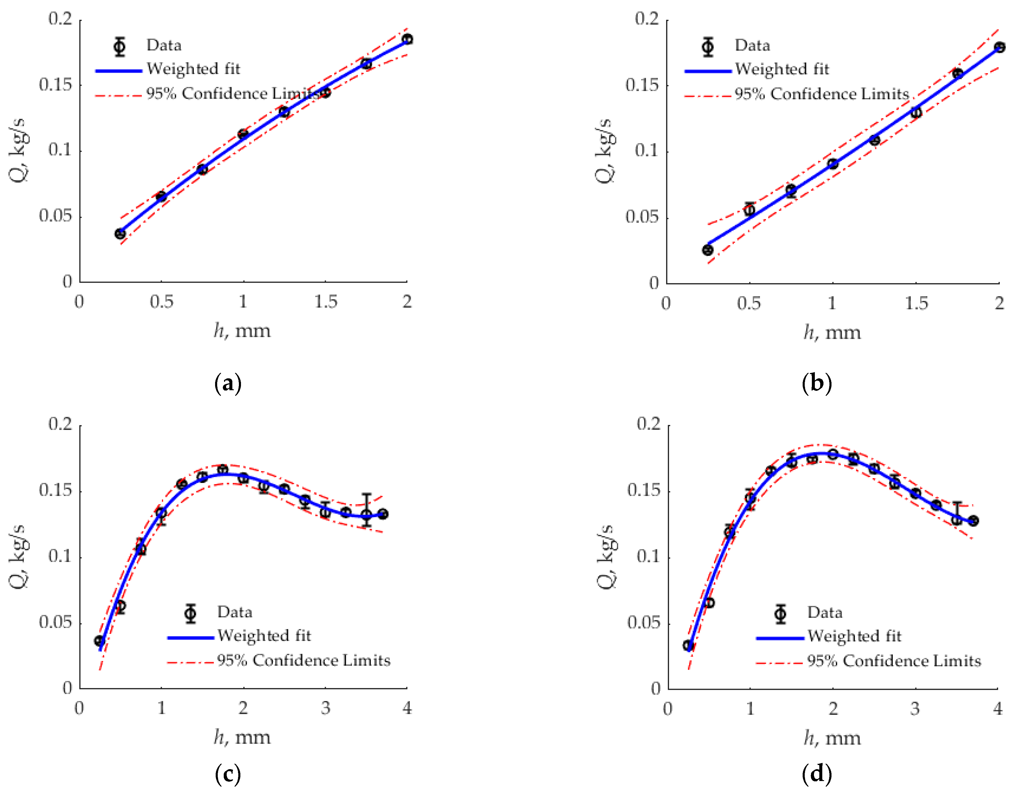
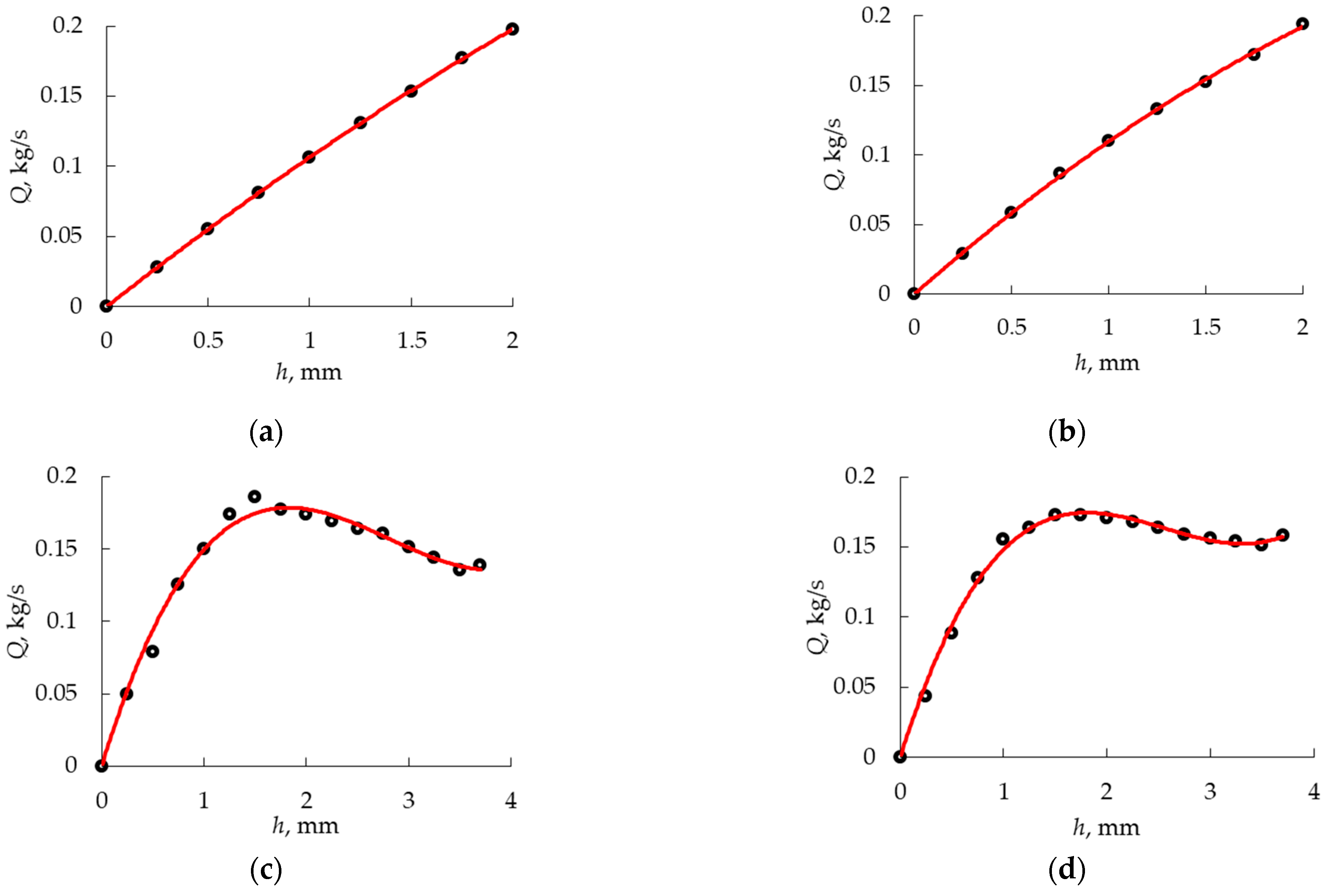
3.1. Experimental Static Flow Characteristics of the Main and Additional Supply Tracts

The static characteristics of the main and additional tracts were determined using the measurement methodology presented in Section 2.2. The opening of both supply tracts was considered in the entire adjustment range, while the direction of supply to the connections related to braking and debraking the output connection connected directly to the executive body (the pneumatic brake system actuator activating the trailer brakes) was also taken into account. To determine the static characteristics of all cases, scatter plots containing the upper and lower measurement deviation of the determined MFR value from five repetitions were used and a regression line was fitted, constituting a static characteristic enabling the search for MFR for the remaining degrees of opening in the main and additional sections, with a 95% confidence level shown by the red line in Figure 11.

Due to the fact that the same stand was used in the tests, a weighted fitting was possible using the Levenberg–Marquardt method [38,39]. The squares of deviations were iteratively minimized, starting from the starting values of the model. The regression line was fitted using a second-degree polynomial function for the main tract and a third-degree polynomial function for the additional tract (blue line in Figure 11).

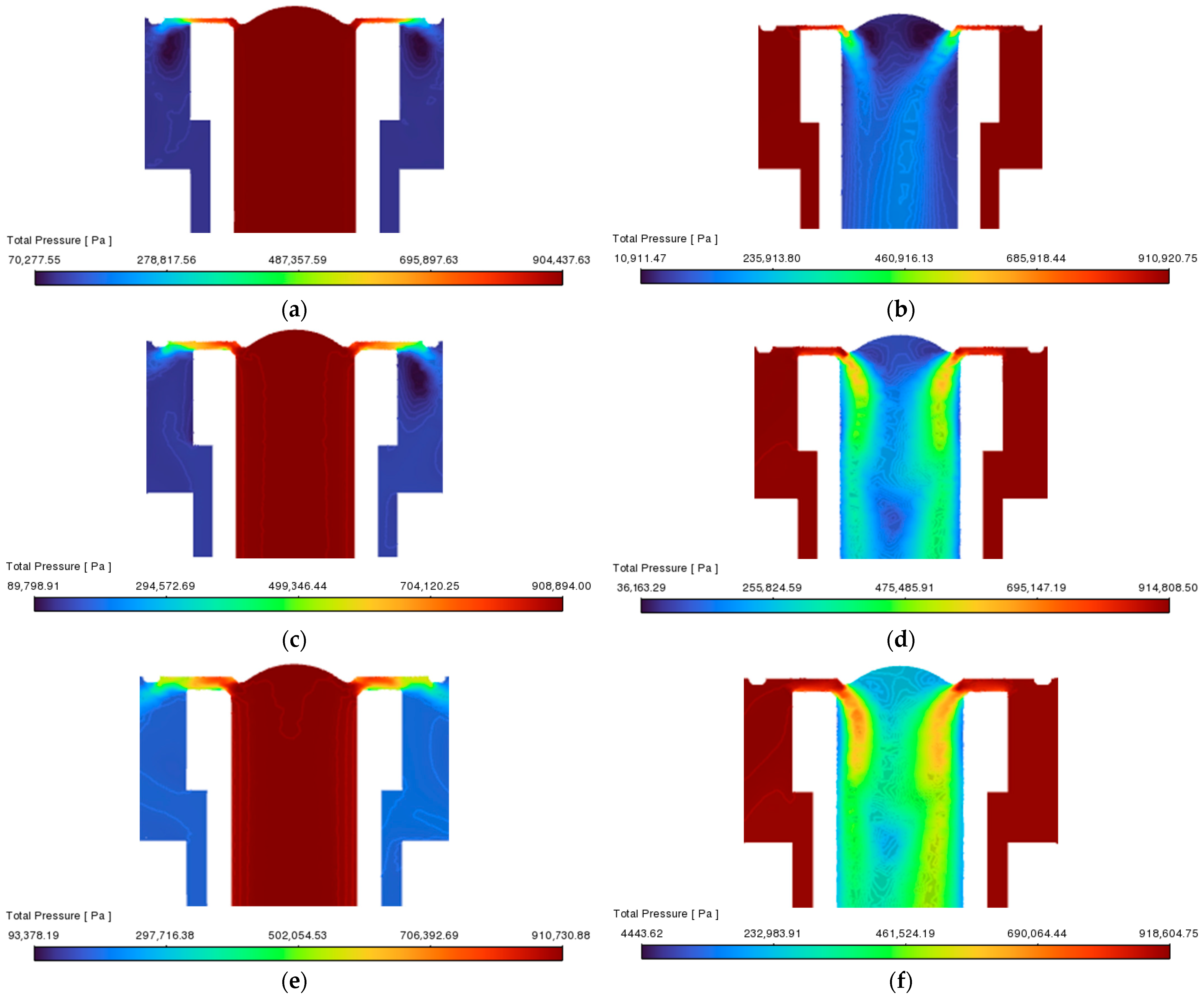
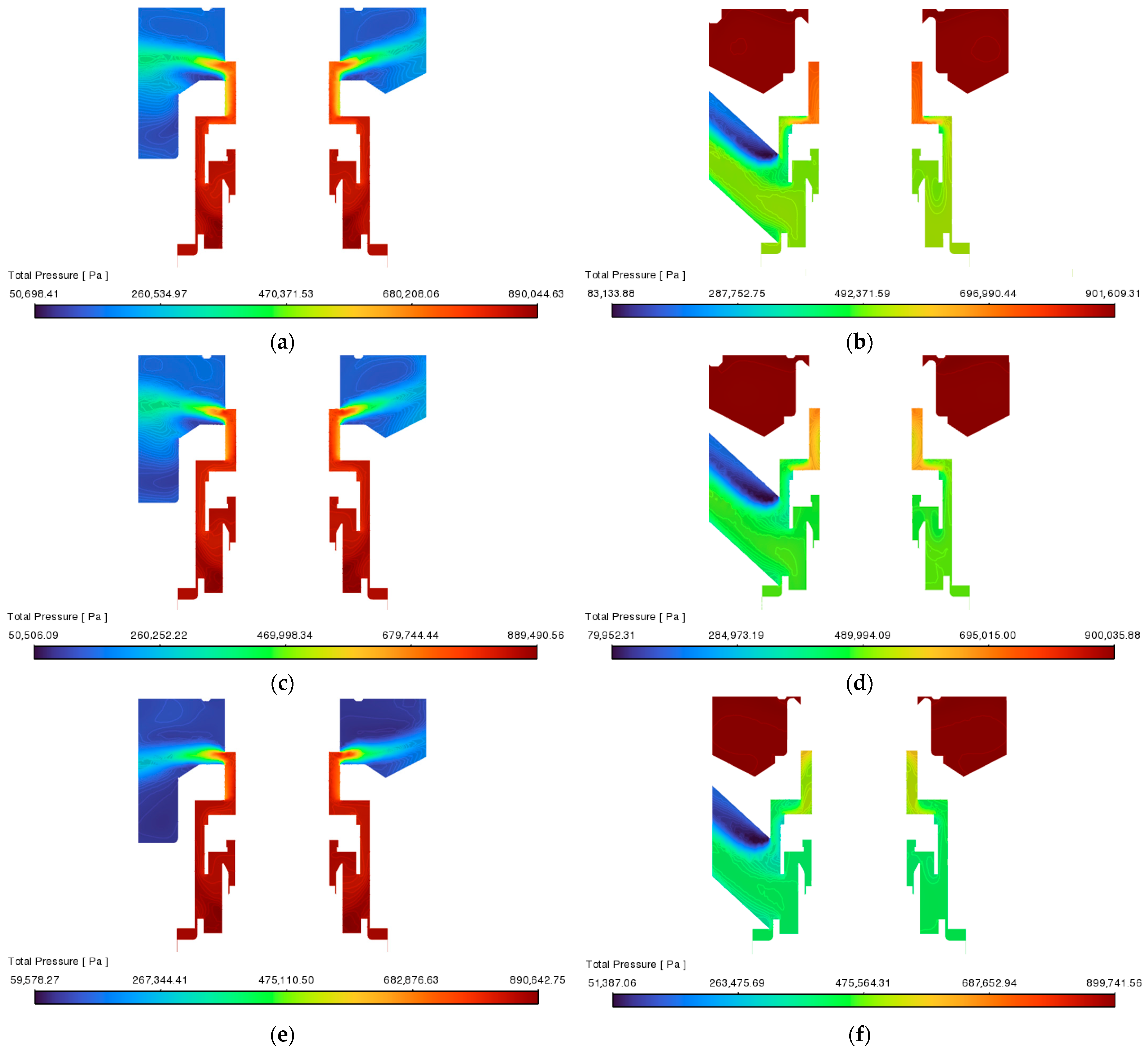
3.2. Numerical Static Flow Characteristics of the Main and Additional Supply Tracts

The determination of the static flow characteristic in the numerical approach was based on the search for a solution to the flow through the internal volume of both supply tracts of the valve based on the developed 3D model. Based on previous analyses [22], it was decided that a polyhedral mesh would be used to discretize the model in accordance with Section 2.3, which, after observing the results, ensured that the numerical method complied with the experimental method adopted as the standard to a certain degree; however, in certain areas, resulting mainly from the small degree of opening in both supply tracts, differences between the two methods are noticeable.

The determination of the static flow characteristics based on the results obtained from Ansys Fluent, similarly to the experimental studies, was possible thanks to the fitting of the regression line based on the obtained values with a polynomial function of the 2nd and 3rd degree, respectively (Figure 12). The use of a polyhedral mesh ensured the optimal simulation time for each considered degree of opening in both tracts.

Examples of the pressure distributions in key flow areas for different degrees of opening in both tracts are shown in Figure 13 and Figure 14. In order to correctly present the pressure distribution in the additional tract, it was necessary to use flow sections in two perpendicular planes, in which the supply and outlet connections were located. The colour map in each section was limited by the minimum and maximum value of total pressure.

The pressure distribution inside the valve chambers shown in Figure 13 and Figure 14 shows the occurrence of local flow accelerations caused by the flow through the narrow channel, which contributes to the formation of local overpressure exceeding the given boundary conditions. The flow through the narrow channel and the Venturi effect also favour the formation of local low pressure areas (negative pressure).

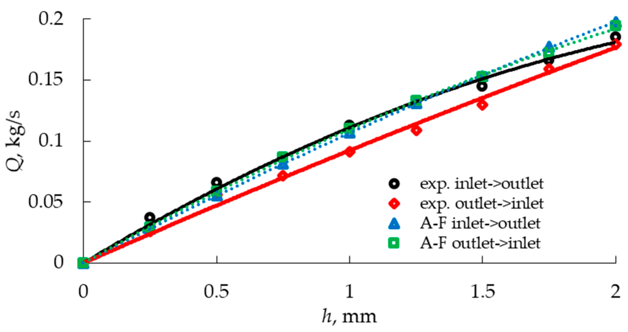
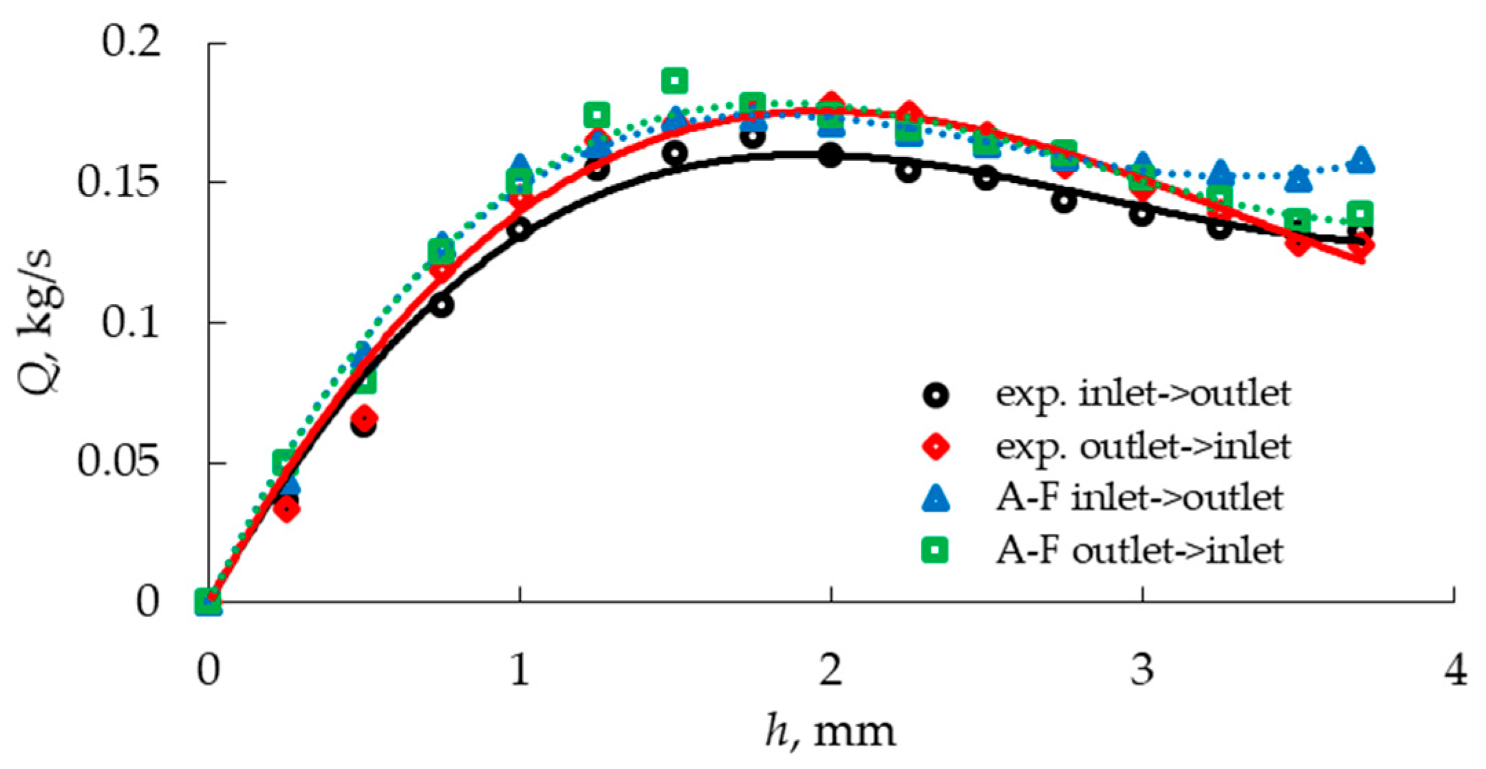
3.3. Comparison of the Static Flow Characteristics Determined Experimentally and Numerically

The determined static characteristics of both tracts providing the tracking and accelerating action of the prototype pneumatic brake valve are presented in Figure 15 for the main path and in Figure 16 for the additional path.

Table 1. MAPE and MAE metrics for main tract—supply from inlet to outlet.

Tract Opening [mm]	0	0.25	0.5	0.75	1	1.25	1.5	1.75	2
Weighted fit	0	0.03158	0.06060	0.08708	0.11100	0.13238	0.15120	0.16748	0.18120
MAPE [%]	0	11%	8%	7%	4%	1%	1%	6%	9%
MAE	0	0.00352	0.00510	0.00596	0.00445	0.00152	0.00190	0.00989	0.01640

,

Table 2. MAPE and MAE metrics for main tract—supply from outlet to inlet.

Tract Opening [mm]	0	0.25	0.5	0.75	1	1.25	1.5	1.75	2
Weighted fit	0	0.02383	0.04715	0.06998	0.09230	0.11413	0.13545	0.15628	0.17660
MAPE [%]	0	22%	25%	23%	19%	16%	13%	10%	10%
MAE	0	0.00524	0.01167	0.01642	0.01776	0.01880	0.01699	0.01568	0.01763

,

Table 3. MAPE and MAE metrics for additional tract—supply from inlet to outlet.

Tract Opening [mm]	0	0.25	0.50	0.75	1.00	1.25	1.50	1.75
Weighted fit	0	0.04526	0.08161	0.10991	0.13100	0.14574	0.15499	0.15959
MAPE [%]	0	10%	4%	14%	15%	19%	20%	11%
MAE	0	0.00167	0.00674	0.01814	0.02451	0.01811	0.01783	0.01346
	2.00	2.25	2.50	2.75	3.00	3.25	3.50	3.70
	0.16040	0.15827	0.15406	0.14862	0.14280	0.13745	0.13344	0.13175
	8%	7%	7%	8%	6%	5%	2%	5%
	0.01065	0.00989	0.00992	0.01056	0.01363	0.01634	0.01800	0.02645

and

Table 4. MAPE and MAE metrics for additional tract—supply from outlet to inlet.

Tract Opening [mm]	0	0.25	0.50	0.75	1.00	1.25	1.50	1.75
Weighted fit	0	0.04710	0.08564	0.11631	0.13980	0.15679	0.16796	0.17400
MAPE [%]	0	6%	8%	8%	7%	11%	11%	2%
MAE	0	0.00269	0.00688	0.00911	0.01031	0.01733	0.01791	0.00316
	2.00	2.25	2.50	2.75	3.00	3.25	3.50	3.70
	0.17560	0.17343	0.16819	0.16055	0.15120	0.14083	0.13011	0.12176
	1%	2%	2%	0%	0%	2%	4%	14%
	0.00171	0.00419	0.00382	0.00004	0.00011	0.00327	0.00560	0.01678

present details of the MAPE and MAE indices for individual valve opening degrees, maintaining both flow directions and referring to the reference characteristic obtained by the experimental method.

4. Discussion

During the experimental tests, a threaded drive was used to determine the position of the control piston h, while the target position was determined by moving the differential tract in conjunction with the pusher (guide). The manual control of the control piston position in the experimental tests presented in the above article required an additional tension spring 17 (Figure 1), which enabled the precise control of the opening of both supply paths. Without a tension spring, the control piston was incorrectly positioned inside the valve working chamber due to friction between the seal and the valve body walls. During the experimental tests, the zero position of the valve was adjusted by observing the pressure in the measuring tank after opening the control solenoid valve. The control piston position was adjusted independently for both paths before each measurement. The adopted method of regulating the degree of opening was the least invasive, with no direct effect on the internal volume of the valve.

A comparison of the static flow characteristics determined by regression lines fitted with a second- and third-degree polynomial function (Figure 15 and Figure 16) shows small differences between the two methods used, while the determined values of MAE and MAPE provide more accurate data. Analyzing the values of these indicators for the main supply tract during braking based on Table 1 shows that the value of the relative error ranged from 1 to 11%. In the entire measurement range, this translates into a discrepancy of 5.88% between the two measurement methods. Considering the same supply tract during release of braking, these discrepancies amounted to 10–25%, which, across the entire measurement range, equated to an average discrepancy of 17.25%. For the additional tract, the relative error values during braking were in the range of 2–20%, giving an average of 9.4%, while during debraking they were in the range of 0–14%, giving an average relative error value of 5.2%. It should be noted that the geometry of the additional tract does not allow for static characteristics close to linear. This is because, with an opening greater than 2 mm, the output flux is reduced, which limits the acceleration effect. This effect was observed in both the experimental and numerical approaches. The small sample size, resulting from the limited number of repetitions of experimental tests and the large capacities of the supplying and measuring tanks, contributed to the use of MAPE and MAE indicators, which, despite their limitations, made it possible to determine the discrepancies between the experimental and numerical approaches.

The adopted simplifications in numerical modelling and the lack of simplifications related to the shape of seals (radius of fillets) in the 3D model had little influence on the quality of the numerical model in Figure 10, determined by the evaluation indices in Ansys Fluent. Compared to the previous numerical studies conducted in a different environment, there are small differences between the numerical methods, while greater possibilities for model discretization; in addition, the possibility of dynamic modelling resulted in focusing on the further use of the Ansys Fluent software only.

The analytical and numerical flow models used required certain simplifications, including adiabatic flow (constant value of inlet and outlet temperature), which excludes the influence of temperature on the results obtained. This is due to the static approach, in which the valve design made it impossible to record changes in the compressed air temperature and the inner wall body without significantly interfering with the structure. Further dynamic studies of the numerical model will take into account the differential (correction) effect of temperature on the valve body and the compressed air near the walls and moving elements.

Further research on the presented conceptual solution of the brake valve with a correction system will focus on dynamic experimental studies. These studies will exclude errors in the regulation of the degree of opening in the supply and additional sections. Previous work by the authors on the influence of selecting the diameter of the channel connecting the working chambers of the correction system will inform the selection of an appropriate configuration for achieving the desired two-range operation. The numerical approach will require the use of dynamic meshes that take into account gas compressibility and the effect of temperature on the mass flow rate. Additionally, other forces in the system must be considered, such as spring tension, inertia, and the friction of the seals against the valve body walls. This approach will enable the evaluation of the operation of the proposed design solution and the use of experimental and numerical methods to determine the reaction time of a pneumatic brake system equipped with a classic relay valve or the valve with a corrective (differential) system proposed by the authors.

5. Conclusions

The use of experimental methods based on the lumped method and numerical CFD in the assessment of the throughput and mass flow rate provides similar results, which was the basis for undertaking this research, with the adoption of certain simplifications enabling the analytical determination of throughput from recorded pressure curves and differential equations based on the lumped method, which has been used repeatedly in the literature to determine pneumatic throughput. No attempts to determine the static characteristics of a pneumatic brake valve using numerical and experimental approaches or to compare both methods were found in the literature.

• It was confirmed that simplifying the flow characteristics of the tracts to a rectangular shape does not reflect the properties of the valves. The applicability of the numerical approach to assessing the flow of brake valve tracts was verified by comparing the values obtained using computer simulation with those obtained using the analytical approach, which has been repeatedly verified in the literature. In earlier studies by the authors, where the nozzle throughput was subjected to experimental and numerical assessment, the differences between the two methods were smaller, mainly due to the geometry of the system, the presence of seals, and the need to introduce a control system to simulate control operations.
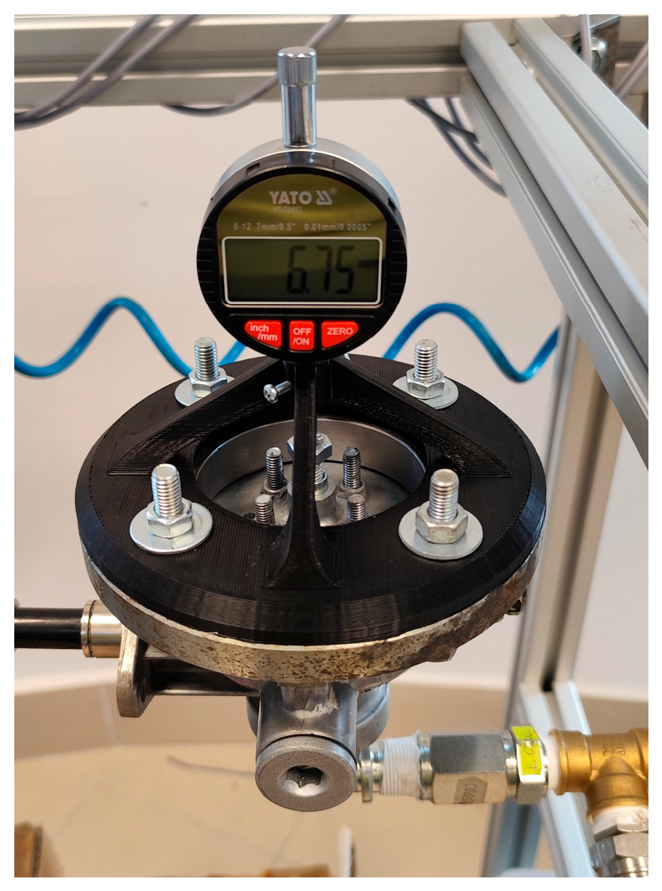
• The movement of the control piston, caused by a sudden increase in pressure at the valve supply port and the piston surface (depending on the flow direction), was observed during the tests. This was the result of the clearance of the threaded connection. Nevertheless, this was the least invasive solution, enabling manual control. It could therefore have had a small impact on the value of the results obtained by the experimental method of this study.
• Preparing the valve’s supply section for experimental tests required the use of additional components to ensure regulation in line with the assumed test conditions. For this purpose, a spring supporting the control piston was used inside the valve body, which ensured the precise adjustment of the piston position and, consequently, the degree of opening of the main or additional supply path.
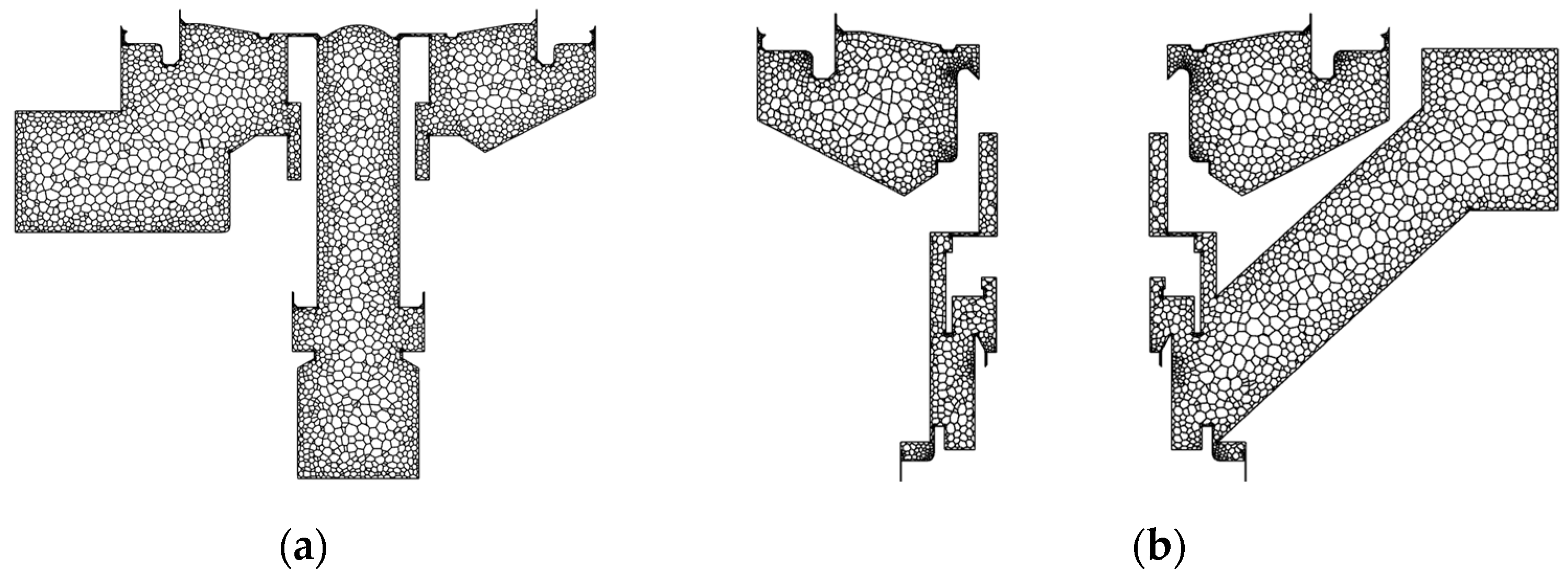
• Numerical tests using a polyhedral mesh with 500 declared iterations and dimensionless residual indicators at 10⁻⁶, representing imbalance in the solver’s differential equations, produced a stable solution, which formed the basis for comparing the results obtained in the numerical and experimental approaches. In numerical modelling, adiabatic flow was assumed, which in real conditions, occurring during experimental tests and the normal operation of the brake valve during service, is a certain simplification. A broader discussion of the impact of temperature on valve operation will form the basis of a dynamic simulation based on multiphysics.
• The discrepancies between both methods assessed using the mean absolute percentage error MAPE were within the range of 0–24%, while the mean value in the entire measurement range was 9.43%, which was mainly influenced by the high MAPE value (17.25%) of the main supply tract during the flow direction resulting from the release of the brake. In the case of a larger sample size, statistical analysis would be necessary, but the aim of the numerical and experimental studies was to assess the possibility of using numerical simulation to determine the pneumatic output of the brake valve, which was achieved by comparing five repetitions of each experimental measurement.
• For the other flow directions of both tracts, the values of the average MAPE index were equal to 5.88%, 9.40% and 5.20%, which proves that, after taking all simplifications into account, the use of simulation methods to evaluate the operation of pneumatic brake valves in a static approach provides satisfactory results.

In future work on the prototype differential valve, the entire valve structure controlled by the operation of the differential section will be subjected to dynamic tests via an experimental and numerical approach.

6. Future Work

The scope of further work on the experimental and numerical analysis of the prototype pneumatic brake valve includes the dynamic evaluation of the operation of both supply tracts caused by the operation of the differential control system. Based on these results, the possibility of its application in a set of vehicles and the verification of dual-range operation, particularly accelerating, will be discussed.

References

1. Cantone, L.; Ottati, A. A Simplified Pneumatic Model for Air Brake of Passenger Trains. Railw. Eng. Sci. 2023, 31, 145–152. [Google Scholar] [CrossRef]
2. Huang, Y.; Yu, L. Research on the Characteristics of a Pneumatic Proportional Valve. J. Phys. Conf. Ser. 2024, 2853, 12043. [Google Scholar] [CrossRef]
3. Dindorf, R.; Takosoglu, J.; Wos, P. Review of Compressed Air Receiver Tanks for Improved Energy Efficiency of Various Pneumatic Systems. Energies 2023, 16, 4153. [Google Scholar] [CrossRef]
4. Li, G.; Wei, X.; Wang, Z.; Bao, H. Study on the Pressure Regulation Method of New Automatic Pressure Regulating Valve in the Electronically Controlled Pneumatic Brake Systems in Commercial Vehicles. Sensors 2022, 22, 4599. [Google Scholar] [CrossRef]
5. Kushaliyev, D.K.; Torebekova, S.O.; Kalshora, E.T.; Korabay, R.B. Analysis of the Main Malfunctions of Hydraulic Cylinders. Bull. L.N. Gumilyov Eurasian Natl. Univ. Tech. Sci. Technol. Ser. 2025, 150, 265–277. [Google Scholar] [CrossRef]
6. Romanoski, V.; Oliveira, L.; Figueiredo, G.; Mayer, M.; Maria, K.; Cavalieri Polizeli, K. Dynamic Soil Hydraulic Properties in Regenerative Agriculture: Effects of Crop and Forest Integration in Livestock Systems. Soil. Tillage Res. 2025, 253, 106680. [Google Scholar] [CrossRef]
7. European Union. Regulation No 13 of the Economic Commission for Europe of the United Nations (UN/ECE)—Uniform Provisions Concerning the Approval of Vehicles of Categories M, N and O with Regard to Breaking [2016/194]; European Union: Brussels, Belgium, 2015. [Google Scholar]
8. Kisiel, M.; Szpica, D.; Czaban, J.; Köten, H. Pneumatic Brake Valves Used in Vehicle Trailers—A Review. Eng. Fail. Anal. 2024, 158, 107942. [Google Scholar] [CrossRef]
9. Kamiński, Z.; Kulikowski, K. Measurement and Evaluation of the Quality of Static Characteristics of Brake Valves for Agricultural Trailers. Measurement 2017, 106, 173–178. [Google Scholar] [CrossRef]
10. Kisiel, M.; Szpica, D. Suboptimal Analysis of the Differential System of the Conceptual Trailer Air Brake Valve. Appl. Sci. 2024, 14, 6792. [Google Scholar] [CrossRef]
11. Kisiel, M.; Szpica, D. Computational Evaluation of the Influence of the Control Piston Bore Throughput on the Differential Action of a Pneumatic Brake Valve. In Proceedings of the 28th International Scientific Conference Transport Means 2024, Kaunas, Lithuania, 2 October 2024. [Google Scholar]
12. Dindorf, R. Measurement of Pneumatic Valve Flow Parameters on the Test Bench with Interchangeable Venturi Tubes and Their Practical Use. Sensors 2023, 23, 6042. [Google Scholar] [CrossRef]
13. Scheaua, F. Theoretical Characteristics of Fluid Flow within a Pneumatic System. Hidraulica 2019, 1, 64–70. [Google Scholar]
14. Kamiński, Z.; Kulikowski, K. Impact of a modified braking valve for static and dynamic characteristics of pneumatic braking systems of agricultural trailers. Int. J. Heavy Veh. Syst. 2021, 28, 291–307. [Google Scholar] [CrossRef]
15. Miatluk, M.; Kamiński, Z.; Czaban, J. Characteristic Features of the Airflow of Pneumatic Elements of Agricultural Vehicles. Commision Mot. Power Ind. Agric. 2003, 3, 174–181. [Google Scholar]
16. Miatluk, M.; Avtuszko, F. Dinamika Pnievmaticeskich i Gidravliceskich Privodov Avtomobilej; Maszinostrojenije: Moscow, Russia, 1980. [Google Scholar]
17. Kaminski, Z. A Simplified Lumped Parameter Model for Pneumatic Tubes. Math. Comput. Model. Dyn. Syst. 2017, 23, 523–535. [Google Scholar] [CrossRef]
18. Bautista, M.; Dufresne, L.; Masson, C. Hybrid Turbulence Models for Atmospheric Flow: A Proper Comparison with RANS Models. E3S Web Conf. 2015, 5, 3001. [Google Scholar] [CrossRef]
19. Sosnowski, M.; Krzywanski, J.; Grabowska, K.; Gnatowska, R. Polyhedral Meshing in Numerical Analysis of Conjugate Heat Transfer. EPJ Web Conf. 2018, 180, 02096. [Google Scholar] [CrossRef]
20. Spiegel, M.; Redel, T.; Zhang, Y.; Struffert, T.; Hornegger, J.; Grossman, R.; Doerfler, A.; Karmonik, C. Tetrahedral vs. Polyhedral Mesh Size Evaluation on Flow Velocity and Wall Shear Stress for Cerebral Hemodynamic Simulation. Comput. Methods Biomech. Biomed. Engin. 2011, 14, 9–22. [Google Scholar] [CrossRef]
21. Yamakawa, M.; Konishi, E.; Matsuno, K.; Asao, S. Adaptive Polyhedral Mesh Generation Method for Compressible Flows. J. Comput. Sci. Technol. 2013, 7, 278–285. [Google Scholar] [CrossRef]
22. Kisiel, M.; Szpica, D.; Czaban, J. Numerical and Experimental Determination of the Bore Throughput Controlling the Operation of the Differential Section of a Pneumatic Brake Valve. Appl. Sci. 2024, 14, 11690. [Google Scholar] [CrossRef]
23. Patil, J.; Palanivelu, S.; Aswar, V.; Sharma, V. Mathematical Model to Evaluate and Optimize the Dynamic Performance of Pneumatic Brake System; SAE Technical Papers 2015; SAE International: Warrendale, PA, USA, 2015. [Google Scholar] [CrossRef]
24. Ren, X.; Lu, Y.; Wang, F. Research on Pneumatic Test System for the Dynamic Characteristic of Hydraulic Solenoid Valve in Brake-by-Wire System. J. Phys. Conf. Ser. 2023, 2674, 12029. [Google Scholar] [CrossRef]
25. Kaminski, Z. Mathematical Modelling of the Trailer Brake Control Valve for Simulation of the Air Brake System of Farm Tractors Equipped with Hydraulically Actuated Brakes. Maint. Reliab. 2014, 16, 637–643. [Google Scholar]
26. Kisiel, M.; Szpica, D.; Czaban, J. Concept of a Test Rig for the Determination of Flow Characteristics of Air Brake Valves in Automatic Cycle. In Proceedings of the 27th International Scientific Conference, Palanga, Lithuania, 4 October 2023; pp. 74–79. [Google Scholar]
27. Szpica, D.; Kisiel, M.; Czaban, J. Simulation Evaluation of the Influence of Selected Geometric Parameters on the Operation of the Pneumatic Braking System of a Trailer with a Differential Valve. Acta Mech. Autom. 2022, 16, 233–241. [Google Scholar] [CrossRef]
28. Miatluk, M.; Czaban, J. Metoda Określania Przewodności Pneumatycznego Regulatora Sił Hamowania Pojazdów. Motrol. Motoryz. Energetyka Rol. 2004, 06, 154–161. [Google Scholar]
29. Kulesza, Z.; Miatluk, M. Analiza Procesów Przejciowych w Pneumatycznym Układzie Hamulcowym z Zaworem Przekanikowym. Arch. Mot. 2008, 1, 33–43. [Google Scholar]
30. Korbut, M.; Szpica, D.; Panão, M. Modelling of Piston Pneumatic Engine Operation Using the Lumped Method. Energy Convers. Manag. 2024, 306, 118310. [Google Scholar] [CrossRef]
31. Chawla, M.; Al-zanaidi, M.A.; Evans, D.J. Linearly Implicit Generalized Trapezoidal Formulas for Nonlinear Differential Equations. Int. J. Comput. Math. 2000, 74, 345–359. [Google Scholar] [CrossRef]
32. Selvam, M.; Manickam, R.; Saravanan, V. Nelder—Mead Simplex Search Method—A Study. In Data Analytics and Artificial Intelligence; REST Publisher: Kaveripattinam, India, 2022; Volume 2, p. 2022. ISBN 978-81-948459-4-2. [Google Scholar]
33. Wang, P.; Shoup, T. Parameter Sensitivity Study of the Nelder–Mead Simplex Method. Adv. Eng. Softw. 2011, 42, 529–533. [Google Scholar] [CrossRef]
34. Marzok, A. Extended Finite Volume Method for Problems with Arbitrary Discontinuities. Comput. Mech. 2025, 1–22. [Google Scholar] [CrossRef]
35. Saeed, A.; Alfawaz, T. Finite Volume Method and Its Applications in Computational Fluid Dynamics. Axioms 2025, 14, 359. [Google Scholar] [CrossRef]
36. Łebek, M.; Panfil, M. Navier-Stokes Equations for Nearly Integrable Quantum Gases. Phys. Rev. Lett. 2025, 134, 010405. [Google Scholar] [CrossRef]
37. Tanaka, K. Air Flow through Suction Valve of Conical Seat: Experimental Research. Part I; Daigaku, T., Kenkyūjo, K., Eds.; Aeronautical Research Institute; Tokyo Imperial University: Bunkyo, Tokyo, 1929. [Google Scholar]
38. Yang, W.; Wang, Y.; Yan, L.; Han, Z.; Gerling, D. Online Detection of Inverter Voltage Error Based on the Voltage Oversampling Measurement and Sigmoidal Function Model. IEEE Trans. Power Electron. 2021, 37, 303–312. [Google Scholar] [CrossRef]
39. Chen, L.; Zeng, R.; Jiang, Z. Nonlinear Dynamical Model of an Automotive Dual Mass Flywheel. Adv. Mech. Eng. 2015, 7, 1687814015589533. [Google Scholar] [CrossRef]
Figure 1. Construction of the supply section of the prototype brake valve: 1—inlet connection, 2—circlip, 3—bushing, 4—spring base, 5, 17—spring, 6, 9, 11, 13—seal, 7—valve body, 8—control piston, 10—middle piston, 12—piston axis guide element, 14—rivet nut, 15—screw, 16—hydraulic plug.
Applsci 15 07483 g001
Figure 2. Method of mounting the valve on the test stand with digital dial gauge.
Applsci 15 07483 g002
Figure 3. Main supply tract.
Applsci 15 07483 g003
Figure 4. Additional supply tract.
Applsci 15 07483 g004
Figure 5. Construction diagram of the test bench: 1—air compressor, 2—pressure regulator, 3, 5, 7, 10—12 VDC electrovalve, 4—choke valve, 6, 9—40.23 × 10⁻³ [m3] tank, 8—tested brake valve regulated with screw, 11–13—voltage pressure transmitter, 14—Raspberry Pi measuring unit, 15—MATLAB 2023 software.
Applsci 15 07483 g005
Figure 6. Test rig view: 1, 4—40.23 × 10⁻³ [m3] tank, 2—24VDC electrovalve, 3—tested brake valve with installed digital dial gauge, 5—Raspberry Pi measuring unit, 6—laptop with MATLAB preinstalled.
Applsci 15 07483 g006
Figure 7. Mathematical diagram of the test rig using the lumped method: p1, p2, p3—instantaneous pressure value, V1, V2, V3—concentrated volume, T = T1 = T2 = T3—temperature (constant).
Applsci 15 07483 g007
Figure 8. Pressure waveforms: (a)—experimental for 0.5 mm opening of main tract; (b)—experimental and model pressure waveforms limited to stable flow.
Applsci 15 07483 g008
Figure 9. Model preparation stages: (a)—view of imported 3D model, (b,d)—extraction of internal flow volume for main (b) and additional (d) tract, (c,e)—view of compressed air volume after suppress all other bodies of 3D model.
Applsci 15 07483 g009
Figure 10. Polyhedral mesh for 0.5 mm opening of (a) main supply tract and (b) additional supply tract.
Applsci 15 07483 g010
Figure 11. Experimental static flow characteristics: (a)—main supply tract from inlet to outlet, (b)—main supply tract from outlet to inlet, (c)—additional supply tract from inlet to outlet, (d)—additional supply tract from outlet to inlet.
Applsci 15 07483 g011
Figure 12. Numerical static flow characteristics: (a)—main supply tract from inlet to outlet, (b)—main supply tract from outlet to inlet, (c)—additional supply tract from inlet to outlet, (d)—additional supply tract from outlet to inlet.
Applsci 15 07483 g012
Figure 13. Pressure distribution of main tract opening: (a,b)—0.5 mm; (c,d)—1.0 mm; (e,f)—1.5 mm.
Applsci 15 07483 g013
Figure 14. Pressure distribution of additional tract opening: (a,b)—1.75 mm; (c,d)—2.50 mm; (e,f)—3.25 mm.
Applsci 15 07483 g014
Figure 15. Experimental and numerical static flow characteristic of main tract.
Applsci 15 07483 g015
Figure 16. Experimental and numerical static flow characteristic of additional tract.
Applsci 15 07483 g016