A Similarity-Based Approach for Diagnosing the Aging of Lithium-Ion Batteries in Second Life Combining Time Series and Machine Learning

Abstract

Modelling aging in the second life of lithium-ion batteries (LiBs) is challenging due to the complexity of degradation mechanisms that lead to capacity loss and internal resistance increase, as well as uncertainty and variability in the operational and environmental conditions to which the batteries are exposed. In this work, we propose a similarity-based approach for diagnosing the aging of LiBs in their second life, which combines time series analysis and machine learning to help identify trends and patterns in the aging process. This approach overcomes the intrinsic nonlinearity nature of the LiB aging trajectory in the second life while adapting to varying operational and environmental conditions. Knees or inflection points defining the first, second, and non-usable lives of the batteries are also identified, offering insights into degradation mechanisms and thus supporting thermal management and optimal user-pattern tasks to extend the LiBs’ lifetime.

1. Introduction

Lithium-ion battery packs used in electric vehicles (EVs) have a lifetime of 4–10 years [1]. The end of life (EoL) in EVs is reached when 20% of the pack’s nominal capacity is lost [2]. The second life of lithium-ion batteries (LiBs) refers to their continued use after retirement from EVs, where ~80% of their capacity remains available but performance is insufficient for automotive use.

The state of health (SOH) of the battery is commonly monitored as the capacity drop over time. This quasi-linear reduction is mostly caused by side reactions in the anode, such as the solid electrolyte interface (SEI) growth and lithium plating (LiP) [3]. These side reactions are known to reduce the ability of lithium ions to intercalate effectively. SEI growth is the dominant side reaction during the first life of the battery, and it is primarily responsible for the quasi-linear reduction in capacity over time, but as it approaches and surpasses the EoL, a nonlinear capacity drop is observed over time due to LiP [4]. In combination, SEI growth and LiP cause further capacity reduction during the second life (after EoL), increasing cell-to-cell variation or capacity spreading among cells [5,6]. Different combinations of stress factors such as temperature, state-of-charge (SOC), depth-of-discharge (DOD), and charge/discharge rate (C-rate) during calendar (at rest) and/or cycling (when charging/discharging the battery) lead to less or more aggressive conditions favouring these side reactions, and consequently, leading to the degradation processes or battery aging, causing the reduced performance [4,7,8]. While it is possible to harvest cell or pack materials right after EoL, extending the operational lifetime of used batteries by giving them a second life provides a secondary revenue stream while reducing the environmental impact of the battery waste [1,9].

In their first life (before EoL), LiBs typically work under a controlled environment, such as in EVs, where management systems regulate charging and discharging and thermal conditions. Modelling aging in first life relies on uniform and consistent data from new cells with known characterizations at the beginning of life. The primary degradation mechanisms in first life are well understood, including SEI growth, lithium plating, and electrode particle cracking, as stress factor values are known and/or recorded, such as C-rates, temperature ranges, and SOC windows, or studied through accelerated aging tests offline. In contrast, in the second life, the battery has already experienced significant degradation and has an aging history. When assembled in secondary applications, such as battery backup systems, heterogeneous aging is introduced, as the repurposed battery has been previously been exposed to varying user behaviors, environmental exposure, and variable aggressive conditions during calendar aging mode (storage). This heterogeneity introduces uncertain degradation history and, hence, variability in initial conditions across cells, modules, and battery packs, which complicates the prediction and diagnosis of future performance, including their remaining useful life. In second life, degradation modes interact, for instance, in nonlinear ways, including complex coupled degradation effects, which are exacerbated by capacity spread among cells. Therefore, the modelling of second life must also contend with data scarcity, high variability, and cell spreading, which cause cell imbalance. These challenges require diagnostic approaches that are interpretable, flexible, scalable, and robust to noise. Thus, the diagnostic focus shifts from predictive SOH to understanding the current battery condition, forecasting its remaining usability, and inferring the causes of past degradation.

It is expected that modelling aging in the second life will follows similar approaches to those used in the first life, including data-based, machine learning, and electrochemically based models [4,10]. Nevertheless, as the contribution of side reactions and other potential mechanisms varies compared to those in the first life, diagnosing aging during the second life can be more challenging. When exploring, developing, and implementing diagnosis approaches in LiBs, researchers focus on quantifying aging mechanisms, predicting the state of health (SOH) as capacity fades, and accounting for cell spreading evolution [5]. Unique and complex challenges arise in second life applications due to the battery’s history, where the pack has been subjected to different user patterns and operating temperatures during its first life, as well as the coupling of several degradation mechanisms with added interaction effects, and cell spreading, which introduces uncertainty when forecasting aging at the module and pack levels. Moreover, while by definition, the window of the second life lies between the first and second knee points of the capacity curve over time, estimating these points remains a challenge [11,12]. Thus, pathways and aging trajectories associated with knee points have different implications for modelling and prediction, and they are impacted by interactions and heterogeneity [12]. Knees-onsets have been predicted using different techniques, including electrochemical, simple data-based (regression), and machine learning techniques [12].

Several approaches have been proposed to predict aging in second life. Thus, Electrochemical Impedance Spectroscopy (EIS) has been used in combination with statistical and machine learning methods, such as Support Vector Machine and K-Nearest Neighbour Regression, to predict the SOH of batteries [13,14], thereby accurately predicting their SOH in the first and second lives. EIS has proven to be effective in clustering aging mechanisms due to side reactions, though it is mostly limited to offline applications [14,15]. Standalone or combined machine learning methods, on the other hand, have been extensively been applied to predict aging in second life as well as remaining useful life, including feature generation and filtering, bagging, deep neural networks, recurrent neural networks, and Long Short-Term Memory (LSTMN) models using online and accelerated test data for different cell chemistries and combinations of stress factors [13,16,17,18]. The limitations of these works are attributed to relying on extensive amounts of data, reduction in accuracy as complexity increases, and computationally expensive models [16,17,18].

The complexity of existing aging prediction models, the inherent limitations of data-driven models, and the need for an understanding of the contribution of different aging mechanisms have led to the conceptualization of an aging diagnosis approach that could offer a trade-off to close these gaps while maintaining accuracy, interpretability, scalability (from cell to pack level), adaptability to different user patterns and stress conditions, and feasibility for real-time or online implementation. An attempt to tackle these challenges included a hybrid aging diagnosis framework in first life, combining kinetically based correlations, time series similarity analysis with side reaction modelling, and remaining useful life (RUL) estimation features [19]. This approach proved reliable in predicting aging contributions and stress factor values, accurate in estimating the contributions of SEI growth and LiP to capacity fade over time, and effective in forecasting RUL [19]. The limitations of the cited work primarily included data dependency, noise sensitivity, and scalability. Nevertheless, the trade-off of this hybrid conceptual approach can be successfully adapted to second life as the principles of aging are retained. At the same time, scalability, or integration into a battery management system, may not be feasible in second life applications. Data dependency will remain a constraint that must be addressed as we gather more aging data.

In this work, we present a similarity-based approach for predicting aging in lithium-ion batteries during their second life, which can capture nonlinear degradation trends and adapting to diverse operational and environmental conditions. Unlike previous works that rely on large, labeled datasets, electrochemical characterization, or computationally intensive machine learning methods, our approach leverages interpretable similarity metrics to map observed aging behavior against known degradation trajectories, providing a practical diagnostic approach that is adaptable to different chemistries, scalable, and straightforward. While this work utilizes synthetic trajectories, these trajectories are derived from kinetic degradation principles and experimentally-observed trends, thereby preserving their real-world applicability. Moreover, our approach is interpretable, as it provides information about aging contributions at a very low computational cost, making it suitable for online applications.

To assess the effectiveness of this approach, we compare five different similarity metrics: two time series-based methods (Dynamic Time Warping and Time Alignment Metric) and three tree-based approaches, including Random Forest similarity, a hybrid Random Forest–DTW method, and an enhanced proximity-tree model. While time series methods are well-suited for capturing temporal distortions and aligning capacity trends, tree-based similarity models offer a powerful alternative, particularly in managing noise and learning complex interactions between degradation features and aging behaviour. Furthermore, tree-based methods inherently provide interpretable proximity measures without relying on temporal alignment as a premise for tracking aging trajectories.

By integrating both types of approaches, our study highlights the complementary strengths of time series and tree-based methods in modelling complex aging behaviour and diagnosing second-life battery health under real-world variability.

2. Materials and Methods

The workflow of our similarity-based approach for predicting the aging of lithium-ion batteries in second life is described as follows:

• Aging datasets must be previously generated from accelerated tests to illustrate aging trajectories (capacity fade over cycle number) defined by several combinations of stress factors. A comprehensive set of cycling and calendar test matrices capturing the operational envelope of LiBs was proposed by [4]. Alternatively, electrochemical-based performance models with embedded aging capabilities (side reactions) can be used to generate aging data artificially [20].
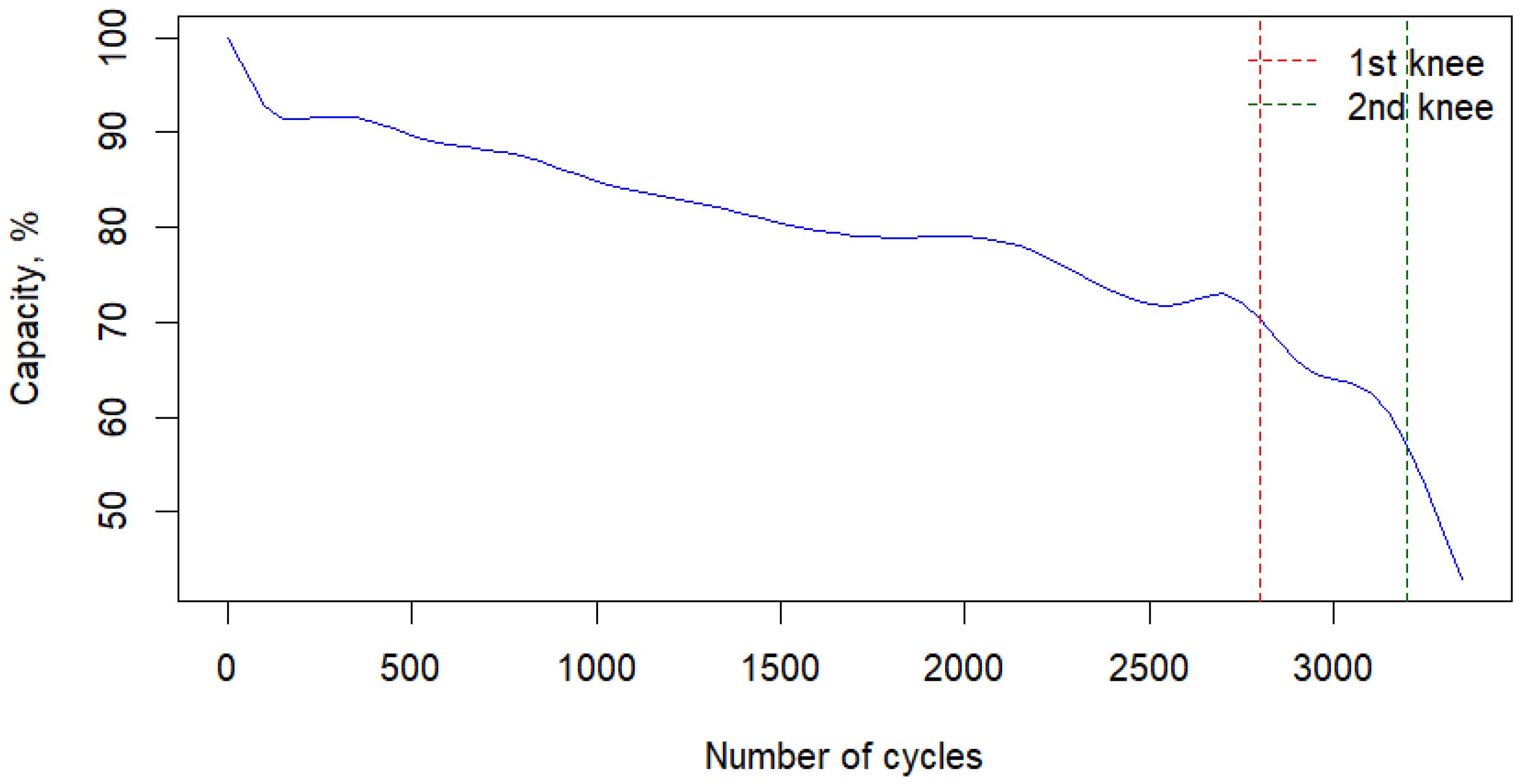
• Knees in each capacity fade curve must be detected to frame the second life window for each trajectory. Therefore, the first knee point of the curve indicates EoL, while the second knee point indicates the battery’s non-useful cycle or time. Second life is then framed between these two knee points, and subsets of the original datasets must be created by extracting the corresponding data within this window.
• Cycling aging curves from real-world second life applications are then compared to each aging trajectory by computing their similarities, and they are later normalized to estimate the contribution percentage of each aging trajectory (associated with a given combination of stress factors) to the cycling aging curve. In this work, we use two approaches to estimate similarity: (i) time series similarity or distance-based similarity approaches and (ii) tree-based similarity approaches. Time series similarity approaches are widely used in different tasks, including clustering, classification, anomaly detection, and forecasting, while tree-based similarity approaches are interpretable, scalable, and can effectively handle complex patterns.

2.1. Dataset, Aging Trajectories, and Synthetic Cycle Generation

This work utilizes a synthetic data generation framework to validate our similarity-based diagnostic approach. The primary objective of using synthetic data is to create testable truth scenarios that define known aging trajectories, where the contribution of stress factors to aging is understood. This allows similarity metrics to decompose a capacity fade curve into several degradation sources.

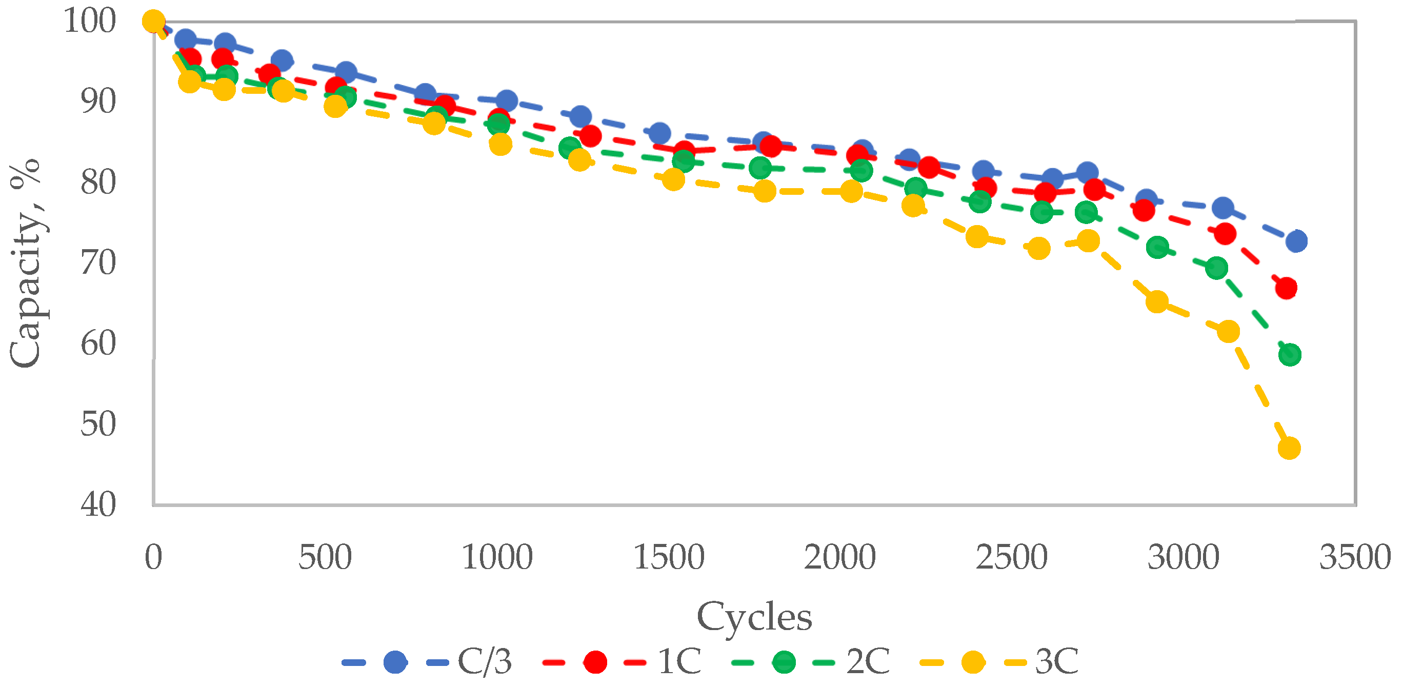
To build our library of aging trajectories, we have selected capacity fade datasets from the literature. Thus, to illustrate how our approach works, we have selected datasets that include modified capacity fade values for NMC622 12.4 Ah pouch cells cycled at 25 °C and four different discharge C-rates (C/3, 1C, 2C, and 3C) [3]. This modification includes interpolated values to maintain the same time scale and added noise. Figure 1 shows the corresponding data points, and the effect of C-rate on capacity fade.

The aging trajectories allow us to verify that the capacity fade increases over the number of cycles as the C-rate increases. Thus, EoL is reached at approximately at 2600 (C/3), 2300 (1C), 2220 (2C), and 1520 (3C) cycles. While we recognize that several other combinations of stress factors shall be available to capture the battery aging phenomenon within a reasonable operational envelope, this work demonstrates our diagnosis approach as a proof-of-concept building on our work presented in [20].

Given the noisy nature of the datasets used in this work, the capacity —as a function of the number of cycles—was fitted using a kinetically based approach employing a modified version of the Dakin equation [4]:

$$C\left(n\right)=C_0\left(1-k{n}^{\alpha }\right)$$

(1)

where $C\left(n\right)$ is the capacity over the number of cycles, $C_0$ is the initial capacity of the cell (assumed as 100 to be associated with the capacity fade percentage), $k$ is the kinetic constant, $\alpha$ is a cycle-dependent factor, and $n$ is the cycle number.

The fitting of the four aging trajectories leads to four estimated values of $k$ and $\alpha$. The noise-free aging trajectories are then generated in the range of approximately 2700 and 4100 cycles (an approximate second life window for the given cells) and are used for comparison against a “real” cycle, which considers these trajectories as capacity time series. In R (version 4.1.1), a well-known data analysis/machine learning software, the nonlinear least squares function, represented as nls (from the stats package, version 4.1.1), was used to fit all these trajectories, leading to relative standard errors ranging from 0.51 and 1.28.

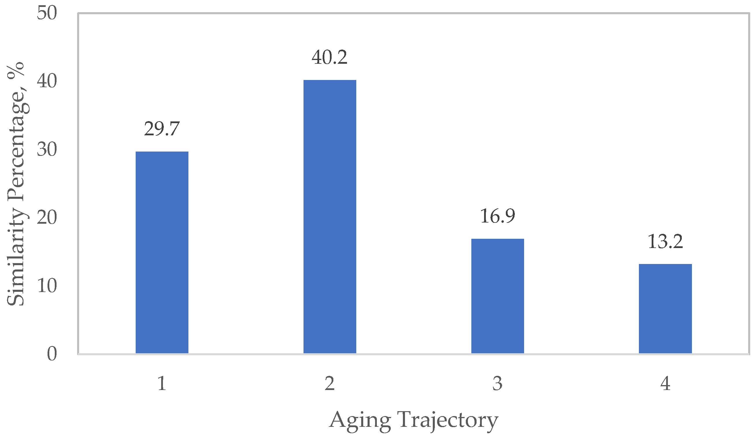
To simulate a realistic second life battery, our computational experiment involved the generating an artificial test cycle, referred to as cycle 1 (

Table A1. Cycle 1 and trajectories 1 to 4 - only second life.

		Trajectory
	Cycle1	1	2	3	4
# cycle	Capacity, %
2700	80.11	80.11	77.81	73.63	69.96
2800	79.29	79.29	76.77	72.37	68.10
2900	78.47	78.47	75.72	71.10	66.21
3000	77.64	77.64	74.65	69.82	64.27
3100	76.52	76.81	73.58	68.53	62.29
3200	75.40	75.98	72.50	67.22	60.26
3300	74.27	75.14	71.41	65.91	58.20
3400	73.12	74.31	70.31	64.58	56.09
3500	71.97	73.47	69.20	63.24	53.95
3600	70.44	72.62	68.09	61.89	51.76
3700	68.89	71.78	66.96	60.53	49.53
3800	67.33	70.93	65.83	59.16	47.27
3900	65.76	70.08	64.69	57.78	44.97
4000	62.33	69.23	63.54	56.39	42.62
4100	58.85	68.37	62.39	54.99	40.24

). This synthetic curve is built as a weighted linear combination of the four noise-free prototype trajectories. These contributions are: 33% from trajectory 1 (C/3), 40% from trajectory 2 (1C), 13% from trajectory 3 (2C), and 13% from trajectory 4 (3C). These weights were selected to reflect a mixed-use second life profile, where the battery experiences from moderate to high stress cycling patterns in both first and second lives. By encoding the contributions of each trajectory, we can evaluate the accuracy of our similarity-based approach in extracting these contributions from the synthetic cycle.

The scope of this study is intentionally limited to the previous trajectories to ensure a controlled evaluation of the similarity-based approach. Our goal here is to first establish the validity of the approach under a well-characterized combination of stress factors before extending to more complex scenarios.

To assess the robustness of our approach under more realistic conditions, we generated noisy versions of cycle 1 by adding Gaussian white noise with increasing standard deviations, ranging from 0.1% to 0.5% of the signal amplitude. This allows us to simulate the data acquisition noise that would eventually occur in real-world applications. Similarity metrics estimated under these conditions allowed us to evaluate the noise tolerance of the proposed approach.

Our computational experimental setup mimics features of real-world second life battery behaviour, including a combination of stress factors, nonlinear degradation, and noise. This controlled validation framework provides proof of concept for our proposed approach and is illustrated in Figure 2.

In aging data generation, we can use experimental or synthetic data in various combinations of stress factors, as well as electrochemical models that incorporate aging. The knee point detection stage allows the identification of the end of life (EoL) and the battery discarding threshold or end of second life. This stage frames the second life window between the knees. Trajectories are then fitted using a kinetics-based approach. In the generation of the synthetic cycle stage, we build a cycle from known trajectory weights; this is the cycle from which the similarity method will recover the true weights. The similarity computation is executed by comparing the generated cycle against the reference trajectories. Normalized contributions are estimated by time series and tree-based similarity methods. In the noise robustness test, we add Gaussian noise to the cycle to evaluate the performance of the methods under realistic noise conditions. The output and diagnosis stage displays the contribution percentage of each aging trajectory, thereby validating our approach in a controlled setting.

2.2. Knees Estimation

The premise of this work is to diagnose the real aging cycle or capacity fade curve of the battery in second life by comparing it against known aging trajectories or predefined cycles, where the combinations of the stress factors leading to the trajectories are known, to estimate the contribution of each combination to the real aging cycle. Known aging trajectories are obtained from accelerated test data, including first and second life, for which an accurate window for second life must be previously estimated. In this work, we employ Bayesian Change Point (BCP) detection, a statistical method used to identify points in a sequence (rate of change), allowing for the detection of knee or elbow points in the capacity fade curve [21]. BCP, unlike clustering, accounts for order and temporal continuity. It has a probabilistic interpretation that supports uncertainty quantification and efficiently detects subtle changes or shifts.

In BCP, the time series is divided into segments, each with its own statistical properties, such as mean and variance. The change point is the unknown time at which these properties change. The Bayesian approach provides a probability distribution for possible change points or knees, considering the uncertainty in the estimate. The likelihood of the observed data is calculated given that there is a knee at some point, and it is assumed that the change is uniform prior. The posterior distribution is obtained using Bayes’ Theorem, which combines the likelihood with the prior. The simplified sequence calculation for BCP is shown as follows [21,22]:

• Given a time series $y_1, y_2,\dots ,y_T$, the goal is to find one or more change points ${\tau }_1, {\tau }_2,\dots$, where the statistical properties of the data change.
• Bayesian methods aim to compute their posterior distribution given the observed data:

$$P\left(\left.\tau \right|y_1:T\right)={\displaystyle \frac{P\left(\left.y_1:T\right|\tau \right)P\left(\tau \right)}{P\left(y_1:T\right)}}$$

(2)

where

$P\left(\left.\tau \right|y_1:T\right)$: Posterior probability of change points;

$P\left(\left.y_1:T\right|\tau \right)$: Likelihood of data given change points;

$P\left(\tau \right)$: Prior distribution over change points;

$P\left(y_1:T\right)$: Marginal likelihood.

• Data is modelled as a piecewise independent segments (likelihood):

$$P\left(\left.y_1:T\right|\tau \right)={\prod }_{i=0}^{k}P\left(\left.y_{{\tau }_i+1:{\tau }_i+1}\right|{\theta }_i\right)$$

(3)

where

${\theta }_i$: Parameters for segment i;

Each segment is assumed to follow a known distribution.

In our R code, the time series is loaded, and the BCP analysis proceeds to detect change points or knees between a threshold onward (set to 0.85) and a change point threshold (set to 0.5) to frame second life. The first knee detection is identified by finding the index where the posterior probability exceeds the threshold of 0.5. After detecting the first knee point, a new subset of data is prepared, and BCP is applied again to this subset. The second-life time series is then obtained by extracting the data between these two knees.

2.3. Time Series Similarity

This section presents the time series methods used for time series similary.

2.3.1. Dynamic Time Warping

Dynamic Time Warping (DTW) is an algorithm used to measure the similarity between two time series by finding the optimal alignment between them by warping the time axis. DTW is based on Euclidean distance, in which a cost matrix between two sequences is built, and a path through the matrix that minimizes the cost path [23]:

• Given two time series or sequences $A=\left(a_1,a_2,\dots ,a_n\right)$ and $B=\left(b_1,b_2,\dots ,b_n\right)$, DTW finds the warping path between these series that minimizes the total distance.
• A cost matrix $D\in {\mathbb{R}}^{n x m}$, where each element is the distance between points (typically Euclidean):

$$D\left(i,j\right)=dist\left(a_i,b_j\right)$$

(4)

• A warping path W is a sequence of matrix indices:

$$W=\left({\omega }_1,{\omega }_2, \dots ,{\omega }_L\right), {\omega }_k=\left(i_k,j_k\right)$$

(5)

Subject to boundary condition ${\omega }_1=\left(1,1\right)$ and ${\omega }_L=\left(n,m\right)$, monotonicity $i_{k+1}\ge i_k,j_{k+1}\ge j_k$, and continuity $i_{k+1}-i_k\le 1,j_{k+1}-j_k\le 1$.

• The optimal is found using dynamic programming:

$$DTW\left(i,j\right)=D\left(i,j\right)+min\left\{\begin{array}{c}DTW\left(i-1,j\right)\\ DTW\left(i, j-1\right)\\ DTW\left(i-1, j-1\right)\end{array}\right.$$

(6)

With initializations $DTW\left(\mathrm{0,0}\right)=0$ and $DTW\left(i,0\right)=DTW\left(0,j\right)=\infty$ for $i,j>0$.

• The final DTW distance is $DTW\left(n,m\right)$.

In our R code, we used the corresponding functions of the library dtw to estimate the DTW distances between time series [24].

2.3.2. Temporal Aggregation of Measures

Temporal Aggregation of Measures (TAM) is a method in which time series are divided into segments, and the similarity of each segment is computed. Then, the scores are aggregated to obtain an overall similarity between two time series [25].

• The time series data is summarized over fixed intervals using aggregation functions such as the mean.
• Similarity measures are then applied to the aggregated series (e.g., DTW or Euclidean distance).
• A similarity score is then calculated based on the chosen metric, reflecting the degree of matching to it. In our case, we chose cross-correlation (maximum absolute value from the cross-correlation function), since this metric is computationally efficient and effective when comparing trends or patterns rather than exact values between time series [26].

In our R code, we followed the previous steps to estimate the similarity score using the correlation between time series.

2.4. Tree-Based Methods for Similarity

This section presents the tree-based methods used for time series similary.

2.4.1. Random Forest

Random forest (RF) builds several trees; for each pair of input time series (A, B), similarity is defined as the number of trees where A and B end up in the same leaf node. We first extract features from time series, train an RF classifier, and estimate the proximity matrix where the similarity is searched. We build a forest of decision trees trained on a bootstrap sample of the data; consequently, some observations will end up in the same terminal node, co-occurrences will be counted (how many trees end up in the same leaf), and a normalized symmetric matrix will finally be formed with values range from 0 (never together) to 1 (always together) [27].

In our R code, we use the package randomForest and its corresponding functions to create a feature matrix (with DTW distances to handle nonlinear temporal relationships effectively), train the random forest model, and extract the proximity matrix (where values range from 0 to 1, with 1 being the more similar) [27].

2.4.2. Proximity in Random Forest Terminal Nodes

This approach, named PRFTN, is a modification of the RF code whose similarity basis is the proximity in RF terminal nodes. It uses full capacity curves as predictors, with each time step defined as a feature. RF learns from raw capacity curves to classify series and finally computes the proximity matrix from terminal node co-occurrence in RF. This RF modification offers faster performance, focusing on understanding terminal node groupings and interpreting the forest structure. In contrast, the RF-DTW utilizes time warping to obtain better shape matching. The simplified math supporting this approach is summarized as follows:

• The cycling aging data and aging trajectories’ capacities are stacked into a matrix, where each row is labeled by its class.
• An RF classifier is trained to distinguish the capacity values (features) among all time series. The RF is composed of a given number of trees $T$, and each tree outputs terminal node assignments.
• A proximity matrix $P\in {\mathbb{R}}^{nxn}$ is defined as:

$$P_{i,j}={\displaystyle \frac{1}{T}}{\sum }_{t=1}^{T}1\left({Node}_{i,t}={Node}_{j,t}\right)$$

(7)

Denoting the proportion of trees where samples i and j land in the same terminal node. A similarity score is estimated between every pair of samples.

• The raw similarities of the cycling data to each aging trajectory are extracted and normalized to sum to 100% [27].

3. Results

This section presents the results of our similarity-based diagnosis using a synthetic second life cycle.

3.1. Knees Estimation

Figure 3 illustrates the knee points for the aging trajectory 4 (2C).

The first knee point (EoL) was estimated at 2800 cycles with a posterior probability of 0.64 (or 64% confidence based on the Bayesian analysis), and the second knee point (non-useful point) at 3200 cycles with a posterior probability of 0.45 (or 45% confidence based on the Bayesian analysis). Results require further validation, as the second knee point has low confidence. Hence, this estimate should be treated cautiously. As a rule of thumb, making sound decisions aims for ≥80% confidence, while modelling aims at 60–80% confidence to be acceptable. Similar behaviour is observed in all aging trajectories, for which we hypothesize that the aging curve is noisy near the second knee point or that there are fewer observations in this region.

3.2. Time Series Similarity

This section includes the similarity results from the time series similarity methods.

3.2.1. Dynamic Time Warping

Figure 4 shows the similarity percentages using DTW between cycle 1 and aging trajectories 1 to 4, illustrating the contribution percentage of each aging trajectory (associated with a given combination of stress factors) to the cycling aging curve.

3.2.2. Temporal Aggregation of Measures

Figure 5 shows the similarity percentages using Temporal Aggregation of Measures (TAM) between cycle 1 and aging trajectories 1 to 4, illustrating the contribution percentage of each aging trajectory (associated with a given combination of stress factors) to the cycling aging curve.

3.3. Tree-Based Methods for Similarity

This section includes the similarity results from the tree-based similarity methods.

3.3.1. Random Forest

Figure 6 shows the similarity percentages using RF between cycle 1 and aging trajectories 1 to 4, illustrating the contribution percentage of each aging trajectory (associated with a given combination of stress factors) to the cycling aging curve.

The similarity percentages are nearly uniform across all four trajectories, indicating the consistency of this method across various aging patterns.

3.3.2. Random Forest with Dynamic Time Warping

Figure 7 shows the similarity percentages using RF with DTW between cycle 1 and aging trajectories 1 to 4, illustrating the contribution percentage of each aging trajectory (associated with a given combination of stress factors) to the cycling aging curve.

In this combined approach, pairwise DTW distances between all trajectory pairs are first computed and then converted to similarity scores in the range [0, 1], with a higher similarity score indicating a closer alignment within the curves. An RF is built using the similarity matrix as features and labels as the target. Finally, the RF proximities are extracted. The main advantage of this approach lies in leveraging the alignment and classification synergy between these two methods, as well as preprocessing similarity through DTW, to enable the RF to learn from pairwise similarities.

3.3.3. Proximity in Random Forest Terminal Nodes

Figure 8 shows the similarity percentages using Proximity in Random Forest terminal nodes (PRFTN) between cycle 1 and aging trajectories 1 to 4, illustrating the contribution percentage of each aging trajectory (associated with a given combination of stress factors) to the cycling aging curve.

3.4. Comparison Between Similarity Methods

Table 1. Comparison between similarity methods.

Aging Trajectory	Time Series				Tree-Based
	DTW	% Error	TAM	% Error	RF	% Error	RF-DTW	% Error	PRFTN	% Error
1	29.7	−3.6	25.8	−7.5	26.3	−7.0	29.1	−4.3	41.6	8.3
2	40.2	0.2	25.8	−14.2	25.9	−14.1	36.1	−3.9	37.4	−−2.6
3	16.9	−23.1	25.8	−14.2	24.4	−15.6	19.5	−20.5	18.3	−27.6
4	13.2	−26.8	22.6	−17.4	23.4	−16.6	15.3	−24.7	2.7	−37.3
Weighted average error, %		−7.8		−12.4		−12.3		−9.0		−6.2

presents a comparison of each similarity method when comparing cycle 1 against aging trajectories 1 to 4 in terms of the absolute error and weighted average error.

Figure 9 allows comparing the similarity percentages among all tested methods.

Figure 9a compares DTW and TAM methods against the real trajectory. DTW shows a similarity with trajectory 2 (~40%), while TAM shows better performance compared to trajectories 3 and 4. Figure 9b compares the tree-based methods (RF, RF-DTW, and PRFTN). PRFTN shows high similarity for Trajectory 1 (~40%), while RF and RF-DTWN align closely with trajectories 1 and 2 but underperform on trajectories 3 and 4.

4. Discussion and Final Remarks

This section presents the discussion of our similarity-based diagnosis using a synthetic second life cycle.

4.1. General Discussion

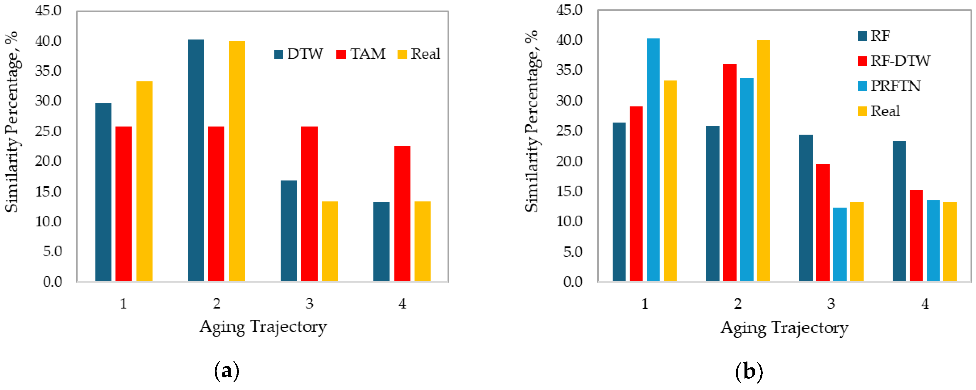
Among the time series methods, DTW shows the closest approximation to the actual similarity percentages (in cycle 1) across three out of four trajectories. Thus, DTW performs well when estimating the contribution percentage of aging trajectory 2 (error of 0.2%) but drops to −23.1% and −26.8% for aging trajectories 3 and 4, respectively. In contrast, TAM shows consistent but larger deviations from the actual similarity percentages. The weighted average error for DTW is −7.8%, substantially lower than TAM’s −12.8%, indicating a better overall alignment with the actual data. DTW is believed to perform well in certain cases when trajectories follow similar shapes but are shifted or stretched in time/cycles while dynamically aligning sequences, making it suitable for misaligned phases. However, this method is quite sensitive to local fluctuations, which could explain the errors estimated when comparing cycle 1 to aging trajectories 3 and 4. On the other hand, TAM underperforms as it utilizes linear segment alignments that may not capture nonlinear aging behaviours or, due to providing more conservative alignments, leads to lower accuracy.

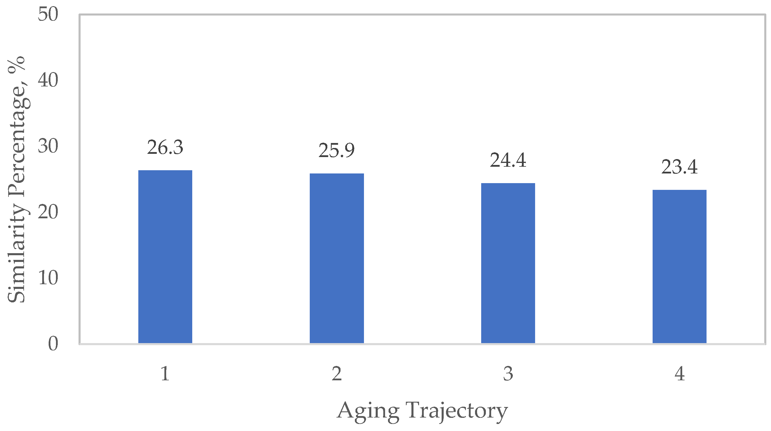
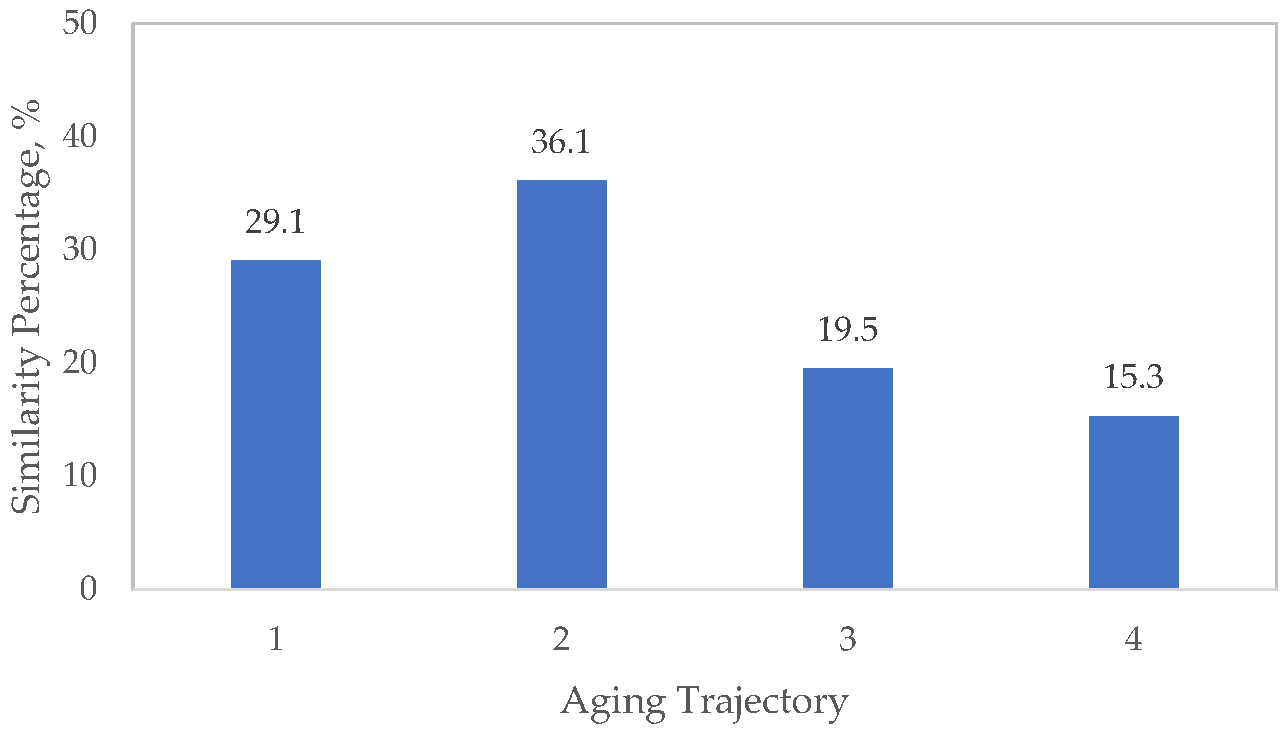
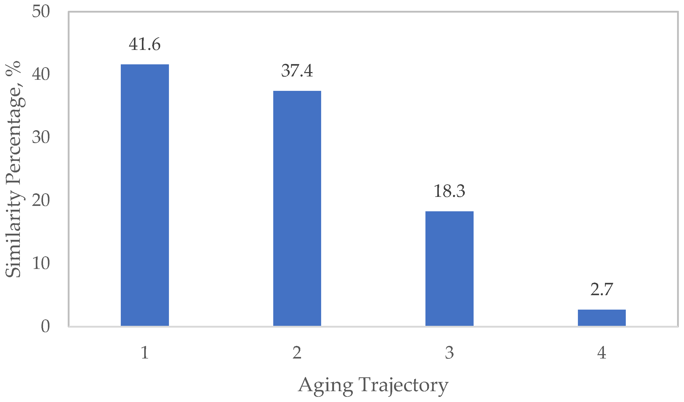
Regarding the tree-based methods, PRFTN performs the best, with a weighted average error of −6.2%, outperforming RF (−12.3%) and RF-DTW (−9.0%). Nevertheless, PRFTN also reported the highest absolute error among all trajectories and methods for trajectory 4 (−37.3%). A unique feature of this comparison is the highest similarity percentage error of 41.6%, estimated by PRFTN for trajectory 1, which suggests a higher sensitivity to certain trajectory features. While the following lowest absolute error is for DTW, a model robustness analysis to noise for DTW and RF-DWT reveals that adding Gaussian noise to the capacity included in the cycle (from the standard deviation of 0 to 0.5) increases the weighted average error to 1.9% for DTW and 0.7% for RF-DTW. RF-DTW tends to be more robust to noise than pure DTW, as merging RF into DTW helps ensemble smoothing, due to bootstrapping and aggregation decisions from many trees, a better generalization since trees are trained on subsets of samples.

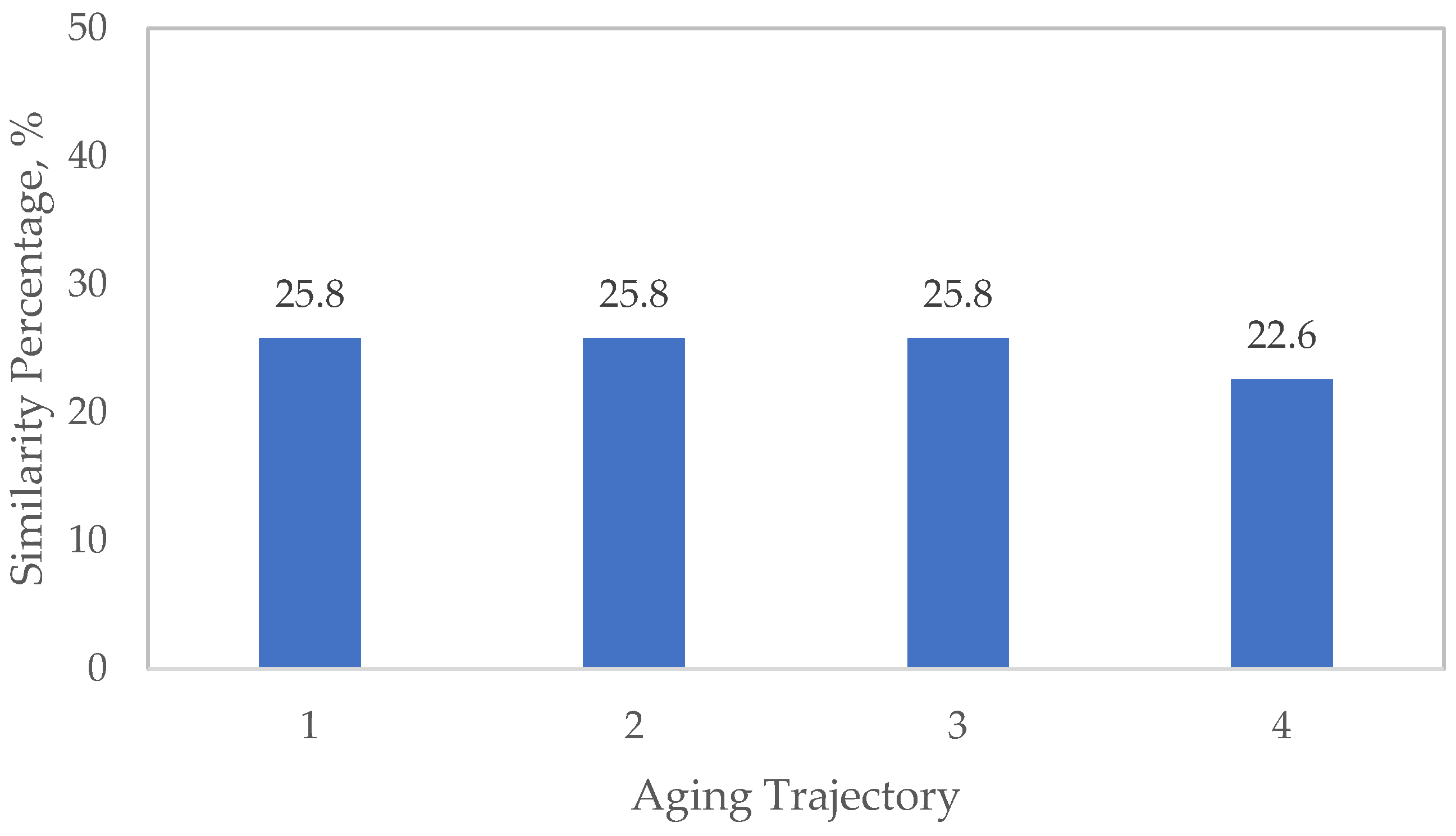
Equal distributions of contributions are observed for RF and TAM. RF can be affected by shallow trees and uniform terminal nodes, while TAM is influenced by over-aggregation and poor/wide aggregation windows, potentially leading to flat similarities.

Across all methods, aging trajectory 2 is the most accurately estimated, while aging trajectory 4 is consistently the most challenging for all methods, exhibiting considerably large negative errors. Tree-based methods generally show less variability across trajectories than time series methods, indicating better generalization.

While the previous discussion pertains to cycle 1, similar findings and trends were observed across several artificially generated cycles, with absolute errors ranging from −40 to 10%.

Our discussion led us to select RF-DTW as the most reliable similarity-based method for diagnosing the aging of lithium-ion batteries in second life, based on the aging trajectories evaluated in this work.

Another alternative to standalone similarity-based methods is the use of hybrid approaches, which combine two or more of the previous methods. Thus, a stacking ensemble is proposed, utilizing linear regression to combine the predictions of multiple similarity-based methods for trajectory analysis. The true similarity score is obtained by combining multiple similarity metrics as follows: (i) calculation of the prediction performance for all pairs of methods using the root mean square error (RMSE), (ii) selection of the best-performing pair (lowest RMSE), (iii) training a linear model on that pair to stack their predictions, and (iv) normalization of the results as percentages.

Table 2. RMSE of pairwise model combinations for similarity prediction.

Model 1	Model 2	RMSE
TAM	RF-DTW	0.6
DTW	TAM	0.9
DTW	RF-DTW	1.7
DTW	PRFTN	2.4
DTW	RF	2.5
RF-DTW	PRFTN	2.8
RF	RF-DTW	3.1
TAM	PRFTN	5.0
TAM	RF	5.3
RF	PRFTN	6.1

summarizes the RMSE for each pair of methods for cycle 1.

The best pair for cycle 1 corresponds to TAM and RF-DTW, likely because they provide diverse yet interpretable signals about the true similarity, combining strengths such as stability (TAM) and capturing variations (RF-DTW). The estimated stacked percentages are 29.1, 40.5, 13.4, 17.0%, compared to 33% from trajectory 1 (C/3), 40% from trajectory 2 (1C), 13% from trajectory 3 (2C), and 13% from trajectory 4 (3C).

Additionally, overall user patterns can be inferred from our diagnosis approach. Thus, at the end of the second life, for instance, RF-DTW estimated that cycle 1 operated at an average C-rate of 1.3C compared to an actual value of 1.2C, based on the contribution of the four aging trajectories. A diverse definition of aging trajectories, based on the combination of stress factors such as temperature, state-of-charge, depth-of-discharge, and C-rate, can potentially provide users with insights into aging that contribute to a better understanding of the battery’s state-of-health (SOH) [20].

Although our current validation relies on synthetic data, there are strong reasons to support the generalization of our similarity-based diagnostic approach to real-world second life battery data. Our approach does not depend on where or how the data has been generated but, instead, on the trends and shape of degradation, which are patterns that can be analyzed across different chemistries when appropriately normalized. Unlike existing ML approaches that require training on specific datasets, our approach does not require retraining on real-world data, as it compares cycles against existing trajectories using interpretable similarity metrics, such as DTW and RF-based proximity. These methods are unsupervised; hence, they are robust to domain shifts since our approach is a diagnostic lookup rather than a black-box predictor. Moreover, aging contributions are mapped to stressors, which is relevant when applied to real-world data. As more trajectories become available, our approach becomes more extensible and specific without requiring structural redesign. Finally, the low complexity and interpretability of our approach make it a suitable candidate for real-time diagnostics, which is a key requirement in second life applications where data availability may be limited.

4.2. Limitations and Future Work

As demonstrated in a previous study [21], aging trajectories should fall within a suitable operational envelope, leading to the main [16] aging mechanisms, for which an extensive number of aging trajectories is required. Therefore, our diagnosis approach depends on reliable and extensive accelerated test data. These trajectories can be generated using electrochemically based models to predict aging and performance. Another consideration when applying our approach is the treatment of noise and outliers in the aging trajectory [20], which may mislead the trajectories. Finally, uneven exposure to aging stress factors might lead to cell spreading, which, specifically in the second life, must be accounted for to ensure scalability from the cell to the pack level. Although this is a proof-of-concept, we plan to obtain additional battery aging data to expand the aging trajectories in future work. We recommend conducting post-mortem analyses to confirm the knee points based on measurable side reaction contributions to aging and cell spreading trends.

The strength of our approach proposed in this work lies in leveraging both interpretable and performance-oriented machine learning tools through aging trajectory contributions to decompose a real cycle. Nevertheless, we plan for future work considering (i) simulating aging trajectories, including combinations of temperature, SOC ranges, DOD, and calendar aging effects, (ii) validating our approach with publicly available data, and (iii) evaluating the effect of spreading (aggregating trajectories) at the module level to simulate pack behaviour [5]. Thus, we will focus on extending the validation of our approach using extensive datasets obtained from real-world applications. This validation is crucial to assess the approach’s effectiveness under different combinations of stress factors, including SOC windows, DODs, and calendar effects. As we consider the feasibility of generalizing our approach, we plan to apply it to different chemistries. Moreover, the similarity-based architecture is inherently adaptable to other energy storage technologies, such as supercapacitors; for this, a tailored library of degradation trajectories must be obtained for specific failure modes and aging signatures.

Potential misclassification due to high diversity is a special consideration when obtaining aging trajectories. For instance, two completely different combinations of stress factors may result in nearly identical aging trajectories, a phenomenon known as trajectory degeneracy. Since our approach aims to classify based on stress factors using only aging curves, the capacity versus cycle is no longer uniquely informative, affecting RF accuracy and proximity-based methods that rely on decision boundaries in a feature space or class separability. To minimize the impact of trajectory degeneracy, we recommend including information about the data as a feature in the aging trajectory datasets to distinguish similar trajectories.

Our diagnosis approach and considerations for future work provide a basis for its scalability, as each aging trajectory represents an independent aging stress path. It is easily modularizable with new data and effective for online implementation. Once trained, trajectory-based diagnosis can be easily matched to incoming cycles online, enabling real-time inference and reliable aging diagnosis while maintaining a low computational cost.

5. Conclusions

In this study, we developed a similarity-based diagnostic approach for assessing aging in lithium-ion batteries during second life. Unlike conventional machine learning (ML) methods that rely on large, labeled datasets, intensive computational resources, or electrochemical characterization, our approach leverages interpretable similarity metrics to map observed aging behavior against known degradation trajectories, offering a pragmatic and generalizable diagnostic approach that can be extended to different chemistries and potentially other energy storage technologies. Five similarity methods were evaluated, including two time series-based and three tree-based approaches, demonstrating that Random Forest combined with Dynamic Time Warping offers the best trade-off between accuracy and robustness.

We also employed a hybrid stacking approach, combining multiple similarity-based methods with linear regression to enhance our similarity analysis. Thus, the best-performing method pair is selected based on the root mean squared error (RMSE) and then used to train the combined model. For cycle 1, the Temporal Aggregation of Measures and Random Forest combined with Dynamic Time Warping yielded the best results, producing similarity percentages that closely matched the ground truth values of contributions.

Based on our results, the proposed approach can effectively estimate the contribution of degradation trajectories. Although the current validation is based on synthetic data, our approach is generalizable to real-world settings, as it relies on interpretable similarity rather than black-box prediction (as in ML methods), making it well-suited for applications in battery second life, which are often challenged by limited historical data as well as uncertain and varying degradation paths.

Future work will focus on expanding the trajectory library to include combinations of additional stress factors (e.g., depth-of-dischagre, state-of-charge, and calendar aging), and consequently validating the performance of our approach using real-world datasets, as well as exploring its applicability to other energy storage technologies, such as supercapacitors.