Dynamic Coal Flow-Based Energy Consumption Optimization of Scraper Conveyor

Abstract

Fully mechanized mining involves high energy consumption, particularly during cutting and transportation. Scraper conveyors, crucial for coal transport, face energy efficiency challenges due to the lack of accurate dynamic coal flow models, which restricts precise energy estimation and optimization. This study constructs dynamic coal flow and scraper conveyor energy efficiency models to analyze the impact of multiple variables on energy consumption and lump coal rate. A dynamic coal flow model is developed through theoretical derivation and EDEM simulations, validated for parameter settings, boundary conditions, and numerical methods. The multi-objective optimization model for energy consumption is solved using the NSGA-II-ARSBX algorithm, yielding a 33.7% reduction in energy consumption, while the lump coal area is reduced by 27.7%, indicating a trade-off between energy efficiency and coal fragmentation. The analysis shows that increasing traction speed while decreasing scraper chain and drum speeds effectively lowers energy consumption. Conversely, simultaneously increasing both chain and drum speeds helps to maintain lump coal size. The final optimization scheme demonstrates this balance—achieving improved energy efficiency at the cost of increased coal fragmentation. Additional results reveal that decreasing traction speed while increasing chain and drum speeds results in higher energy consumption, while increasing traction speed and reducing chain/drum speeds minimizes energy use but may negatively affect lump coal integrity.

1. Introduction

Coal remains a vital energy source and industrial raw material, playing a fundamental role in ensuring energy security and fostering economic growth [1]. In fully mechanized coal mining, energy consumption is notably high, with cutting and transportation identified as the most energy-intensive stages [2]. Among the various subsystems, mining operations alone account for approximately 25% of the total energy consumption in coal production—the highest proportion among all stages. Additionally, underground material transportation can consume up to 60% of the total mining energy use [3,4]. As the primary equipment for coal transport, the scraper conveyor significantly impacts system efficiency and overall energy consumption [5].

Meanwhile, as coal transport systems undergo intelligent upgrades, operational safety has become an increasingly complex challenge. Ensuring safe operation remains paramount, but beyond safety, sustainability has emerged as a core objective aligned with the principles of Industry 5.0 [6,7]. However, the lack of an accurate dynamic coal flow model limits precise estimation of energy consumption, thereby hindering further optimization and restricting the industry’s potential for substantial energy savings and efficiency improvements. Therefore, achieving a balance among efficient energy use, safety, and sustainability is critical for the future development of coal mining transport systems.

In recent years, researchers have developed various coal flow modeling methods for scraper conveyors to improve energy efficiency and system performance. Yin et al. [8] designed a scraper conveyor load model and a coal volume calculation algorithm based on array modeling, enabling real-time simulation of unit coal volume through multi-parameter mathematical modeling. Hu et al. [9] proposed a laser-scanning-based system for coal release monitoring in fully mechanized caving faces, introducing a regression model for real-time coal volume estimation using the triangular micro-element method. By measuring coal flow on the upper section of the rear scraper conveyor near the discharge opening, this model effectively captured dynamic coal distribution in the working face. Expanding on laser-based modeling approaches, Wang et al. [10] developed a coal-discharge-monitoring system that utilized laser scanning to capture point cloud data of coal flow contours near the discharge opening. Based on these features, a high-precision 3D model of coal accumulation on the scraper conveyor was constructed in real time. Additionally, Chen et al. [11] and Guo et al. [12] introduced a coal flow volume measurement method based on linear model segmentation, improving the accuracy of coal volume estimation. These studies have contributed to refining coal flow models by integrating real-time data acquisition with mathematical modeling techniques.

Although current studies using laser scanning, ultrasonic sensing, and array modeling have improved coal flow modeling, existing models still have limitations. Most rely on simplified assumptions about coal distribution and do not fully account for complex flow behaviors such as accumulation, dissipation, and interactions with the conveyor. Moreover, factors like sensor accuracy, external disturbances, and the model’s adaptability to different operating conditions affect the precision of coal flow modeling.

Significant progress has been made in studying the dynamic characteristics and energy consumption of scraper conveyors. Liu et al. [13] proposed a resistance calculation method based on material distribution characteristics and experimentally verified its effectiveness. Lohning et al. [14] conducted an in-depth study on the operating resistance of scraper conveyors, providing valuable insights for conveyor design and optimization. Dolipski et al. [15] focused on chain tension issues, identifying the smoothness of the drive system startup as a key factor influencing chain tension. They further proposed an algorithm to evaluate the dynamic load of scraper conveyors. Zhang et al. [16] developed an electromechanical coupling model to analyze the dynamic characteristics of scraper conveyors under various conditions, including no-load startup, steady operation, sudden load increase, and chain jamming. The model’s accuracy was validated through experiments. Zhang et al. [17] used simulations to study the dynamic characteristics of scraper conveyors during startup and braking, revealing performance variations in critical operating phases. Chen et al. [18] introduced a “flexible beam + belt element” modeling approach and constructed a rigid–flexible coupling model using RecurDyn(V9R3) software. They conducted dynamic analyses based on coefficient matrices, laying a theoretical foundation for studying conveyor dynamic characteristics. However, existing studies mainly focus on static conditions or isolated performance indicators, lacking a systematic investigation into the relationship between load distribution and energy consumption under dynamic conditions. Additionally, most analyses rely on experiments and simulations, with limited mathematical modeling support. This gap makes it difficult to fully understand the dynamic behavior and energy consumption characteristics of scraper conveyors under complex operating conditions.

Compared to shearers, research on the energy consumption optimization of scraper conveyors remains relatively underdeveloped. Some studies have explored the relationship between coal flow load and energy consumption at different operational stages, proposing strategies to optimize conveyor operation by adjusting the shearer’s speed. However, the theoretical framework for scraper conveyor energy optimization is still lacking, especially when compared to advancements in shearer energy modeling and parameter optimization. In existing research, Chen et al. [19] analyzed coal mass line density, real-time coal volume, and operational resistance at various process stages, preliminarily establishing an energy consumption model to support scraper conveyor optimization. Liu et al. [20] proposed optimizing conveyor speed by adjusting the shearer’s cutting speed based on real-time load variations. In contrast, significant progress has been made in shearer energy optimization. Zheng et al. [21] developed a shearer energy consumption model and proposed an optimization strategy to minimize energy usage in unidirectional mining, reducing overall system energy consumption. Wang et al. [22] analyzed the effects of cutting parameters on specific energy consumption, identifying the optimal ratio of cutting thickness to cutting line spacing, and providing theoretical guidance for performance optimization. Fu et al. [23] further enhanced cutting efficiency by optimizing double-drum motion parameters using a genetic algorithm (GA).

In summary, despite recent advancements in coal flow detection, dynamic analysis, and energy consumption optimization of scraper conveyors, existing studies remain fragmented and lack a systematic mathematical foundation. In particular, the interactions among load distribution, dynamic behavior, and energy consumption under dynamic conditions have not been fully explored. To address these gaps, this study focuses on the following three aspects:

1.

Establishing and validating a dynamic coal flow mathematical model based on scraper conveyor coal flow characteristics.

2.

Analyzing the mechanical properties of the scraper conveyor and developing a corresponding energy consumption model.

3.

Proposing a multi-objective optimization strategy based on the established energy model, evaluating the impact of parameters on energy consumption and lump coal ratio.

The remainder of this paper is organized as follows: Section 2 develops and validates the dynamic coal flow mathematical model. Section 3 analyzes the mechanical characteristics of the scraper conveyor and constructs its energy consumption model. Section 4 presents the optimization algorithm used to solve the multi-objective optimization model. Section 5 discusses the optimization results and examines the influencing factors. Finally, Section 6 concludes this study and outlines directions for future research.

The overall framework of this paper is illustrated in Figure 1.

2. Development of the Dynamic Coal Flow Model and EDEM Simulation

2.1. Construction of Dynamic Coal Flow Model

Coal Mass Distribution Equation and Dynamic Coal Flow Mathematical Model

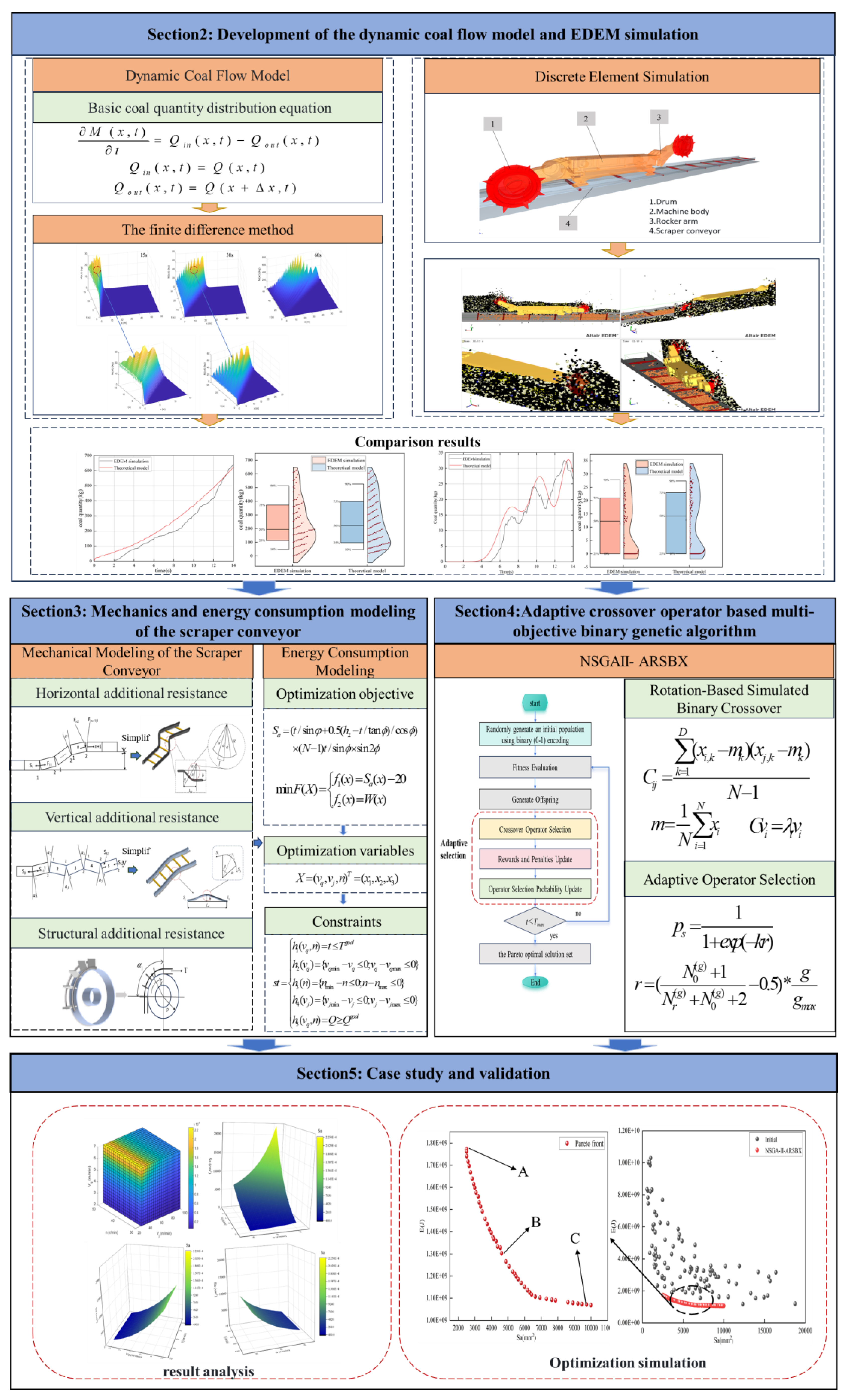
The construction of the coal mass distribution equation and the dynamic coal flow mathematical model is a key foundation for accurately describing the coal transportation process in scraper conveyors. Based on the law of conservation of mass, this model comprehensively considers important characteristics such as accumulation, dispersion, and continuity of coal flow, realistically reflecting the spatiotemporal dynamics of coal flow during mining and transportation. This provides a solid theoretical basis for subsequent energy consumption analysis and optimization. Similar modeling approaches have been widely applied in bulk material transport to characterize mass transfer and transient flow behaviors [24]. The following sections will detail the formulation, derivation, and mathematical representation of the dynamic coal flow model.

1.

Derivation of the coal flow distribution equation

According to the law of mass conservation, the change in coal volume within a given region over time equals the difference between the inflow and outflow coal flow rates, as expressed in Equation (1):

$${\displaystyle \frac{\partial M(x,t)}{\partial t}}=Q_{in}(x,t)-Q_{out}(x,t)$$

(1)

where M(x,t) represents the coal volume distribution at position x and time t, and Q_in(x,t) and Q_out(x,t) represent the inflow and outflow coal flow rates, respectively.

Q(x,t) is defined as the coal flow rate at position x, as shown in Equation (2):

$$Q_{in}(x,t)=Q(x,t) , Q_{out}(x,t)=Q(x+\Delta x,t)$$

(2)

Thus, the equation can be rewritten as given in Equation (3):

$${\displaystyle \frac{\partial M(x,t)}{\partial t}}=Q(x,t)-Q(x+\Delta x,t)$$

(3)

As Δx approaches an infinitesimally small value, Taylor expansion is applied to approximate Q(x + Δx,t) linearly, as given in Equation (4):

$$Q(x+\Delta x,t)\approx Q(x,t)+{\displaystyle \frac{\partial Q(x,t)}{\partial x}}\Delta x$$

(4)

which simplifies to:

$${\displaystyle \frac{\partial M(x,t)}{\partial t}}+{\displaystyle \frac{\partial Q(x,t)}{\partial x}}=0$$

(5)

During coal transportation, the distribution of coal volume varies with both space and time. To develop a mathematical model, coal is treated as a continuous medium on a macroscopic scale, mass conservation is assumed with no external coal input or loss, and the flow is considered one-dimensional along the conveyor, neglecting variations in other directions.

2.

Steady-state coal load equation

According to the coal mass conservation equation, assuming the conveying velocity v(x,t) and the coal flow rate Q(x,t) are locally steady and can be treated as constants, the mass conservation equation can be simplified as follows:

$${\displaystyle \frac{\partial M(x,t)}{\partial t}}+v{\displaystyle \frac{\partial M(x,t)}{\partial x}}=Q(x,t)$$

(6)

Under steady-state conditions, the coal load M(x,t) reaches equilibrium over time; thus:

$${\displaystyle \frac{\partial M(x)}{\partial x}}=0$$

(7)

The equation can be further simplified to:

$$v{\displaystyle \frac{\partial M(x)}{\partial x}}=Q(x)$$

(8)

By integrating this equation, the coal load at any position on the scraper conveyor can be expressed as follows:

$$M(x)=M_0+{\displaystyle \frac{1}{v}}{\displaystyle \underset{0}{\overset{x}{\int }}Q(x^{’})}d{x}^{’}$$

(9)

where M₀ represents the initial coal load.

To better describe the coal accumulation effect, an accumulation factor α is introduced. It is defined as the rate of change in coal load with respect to spatial position x, and is given by:

$$\alpha ={\displaystyle \frac{1}{v}}$$

(10)

A dispersion factor β is used to describe material losses during coal transportation due to friction, collisions, and other factors. It represents the attenuation of coal flow per unit distance and ranges from 0 to 1, reflecting the loss ratio of coal flow during transport. Assuming that coal flow follows an exponential decay pattern during conveying, and that the dissipation rate per unit distance is k, the coal load M(d) after traveling a distance d can be expressed as follows:

$$M(d)=M_0{e}^{-kd}$$

(11)

where k is the dissipation coefficient related to friction, collisions, and other losses, indicating the coal loss rate per unit distance.

Based on the above, the dispersion factor β is defined as the proportion of coal loss per unit distance:

$$\beta =e^{-kd}$$

(12)

Under steady-state conditions, the coal load on the scraper conveyor depends not only on the coal flow rate Q(x), but also on the conveying speed v, the accumulation factor α, and the dispersion factor β. The final expression for calculating the coal load at any point along the conveyor is:

$$M(x)=M_0+{\displaystyle \frac{1}{v}}{\displaystyle \underset{0}{\overset{x}{\int }}(Q(x^{’})-e^{-kd}M(x^{’})})d{x}^{’}$$

(13)

3.

Modification of the dynamic coal flow model

Building upon the coal distribution equation and coal load equation, the relationship between coal flow rate Q(x,t) and coal mass M(x,t) is further explored. It is assumed that the coal flow rate is proportional to the inlet coal mass, given by:

$$M(x,t)={\displaystyle \frac{Q(x,t)}{v(x,t)}}$$

(14)

where v(x,t) is the coal flow velocity at position x and time t, in meters per second (m/s).

Substituting this expression into the coal distribution equation yields the fundamental equation of dynamic coal flow, as shown in Equation (15):

$${\displaystyle \frac{\partial M(x,t)}{\partial t}}+v(x,t){\displaystyle \frac{\partial M(x,t)}{\partial x}}=0$$

(15)

This equation serves as the basic mathematical model for dynamic coal flow, accurately describing the spatial–temporal distribution of coal. However, in addition to mass conservation, the dynamic model must also incorporate the effects of accumulation and dissipation.

The accumulation effect reflects the localized build-up of coal in certain regions, often occurring when the conveyor speed is low or the coal inflow rate is high. To represent this, an accumulation factor α(x,t) is introduced, indicating the accumulation rate of coal flow. The modified coal distribution equation becomes:

$${\displaystyle \frac{\partial M(x,t)}{\partial t}}+{\displaystyle \frac{\partial }{\partial x}}\left(v(x,t)\cdot M(x,t)\right)=\alpha (x,t)\cdot M(x,t)$$

(16)

The dissipation effect describes the gradual reduction in coal flow due to friction, gravity, and other factors during transportation. This is modeled by introducing a dissipation factor β(x,t), representing the coal loss rate:

$${\displaystyle \frac{\partial M(x,t)}{\partial t}}+{\displaystyle \frac{\partial }{\partial x}}\left(v(x,t)\cdot M(x,t)\right)=-\beta (x,t)\cdot M(x,t)$$

(17)

where β(x,t) is influenced by factors such as coal particle size, conveying speed, and friction coefficient.

By incorporating the accumulation factor α(x,t) and dissipation factor β(x,t), the dynamic coal flow equation is further revised as follows:

$${\displaystyle \frac{\partial M(x,t)}{\partial t}}+{\displaystyle \frac{\partial }{\partial x}}\left(v(x,t)\cdot M(x,t)\right)=(\alpha (x,t)-\beta (x,t))\cdot M(x,t)$$

(18)

This equation indicates that the inlet coal flow rate is a key parameter in the dynamic coal flow model, directly determining the evolution and distribution of coal over time and space. The inlet rate is mainly affected by the cutting process of the shearer drum, which governs the volume of coal entering the scraper conveyor per unit time.

As shown in Figure 2, to clearly describe the coal flow formation during drum cutting, a differential surface element is defined in polar coordinates. Let the radius from the drum center to the coal flow be R_i, with small angular increment dθ and radial increment dR_i. Then, a small surface element dA on the drum can be expressed as follows:

$$dA=R_i\times d\theta \times d{R}_i$$

(19)

Thus, the instantaneous volume flow rate V_i at a given time is:

$$V_i={\displaystyle \iint v_i^{\prime }}\cdot dA={\displaystyle {\int }_0^{{\theta }_i}{\displaystyle {\int }_{R_g}^{R_y}\frac{2\pi R_i\times n\times \sin {\alpha }_i\times \cos ({\alpha }_i+\varphi )}{60\cos \varphi }}}{R}_i\times d\theta \times d{R}_i$$

(20)

The instantaneous coal flow rate Q_i generated by the drum can therefore be expressed as follows:

$$Q_i=V_i\times \rho$$

(21)

To ensure that the partial differential equation of the dynamic coal flow model has practical physical significance and can be numerically solved, appropriate boundary and initial conditions are provided.

Inlet boundary condition: the coal flow rate at the inlet of the scraper conveyor, defined as follows:

$$Q(0,t)=Q_{in}(x,t)$$

(22)

Outlet boundary condition: the coal discharge rate at the conveyor’s tail end. This condition ensures accuracy of coal mass at the outlet and maintains continuity with the inlet flow rate:

$$Q(L,t)=Q_{out}(t)$$

(23)

Initial condition: At time t = 0, the initial coal mass distribution within the system is specified. This defines the coal load along the conveyor at the beginning of transport and serves as the initial condition for simulation:

$$M(x,0)=M_0(t)$$

(24)

4.

Numerical solution of the dynamic coal flow model

Numerical methods provide an efficient and reliable means for solving partial differential equations (PDEs) in dynamic coal flow control, particularly when modeling the complex evolution of coal mass over time and space in scraper conveyors. Although PDEs originated in fields such as physics and fluid mechanics, their mathematical foundations were not specifically developed for the coal industry. Nonetheless, numerous studies have successfully applied PDEs in bulk material transport, granular flow, and pneumatic conveying to simulate unsteady flows and mass transfer, thereby validating their modeling capabilities and applicability in multiphysics systems [24,25]. Inspired by these studies, this paper introduces partial differential equations into coal flow modeling and establishes a mathematical model for the spatiotemporal distribution of coal mass based on the principles of mass conservation and flow continuity. Due to the difficulty of obtaining analytical solutions for such models, the Finite Difference Method (FDM) is employed for numerical computation. FDM, as a classic domain discretization technique, transforms PDEs into algebraic difference equations and is frequently used alongside the Finite Element Method (FEM) [26] and the Finite Volume Method (FVM) [27] in scientific and engineering simulations. Among these, FDM is widely adopted for its conceptual clarity and computational efficiency [28,29].

FDM discretizes the physical space into uniform grids and divides the time domain into discrete steps, effectively capturing the spatiotemporal evolution of coal flow during transportation. As noted by Tian et al. (2023) [30], the Finite Difference Method performs well in solving complex boundary and nonlinear problems, and has been extensively applied in key fields such as oil and gas extraction, material transport, and energy delivery. Therefore, the application of FDM to coal flow modeling is not only theoretically sound but also highly feasible in practical engineering contexts.

(1)

Overview of the Finite Difference Method

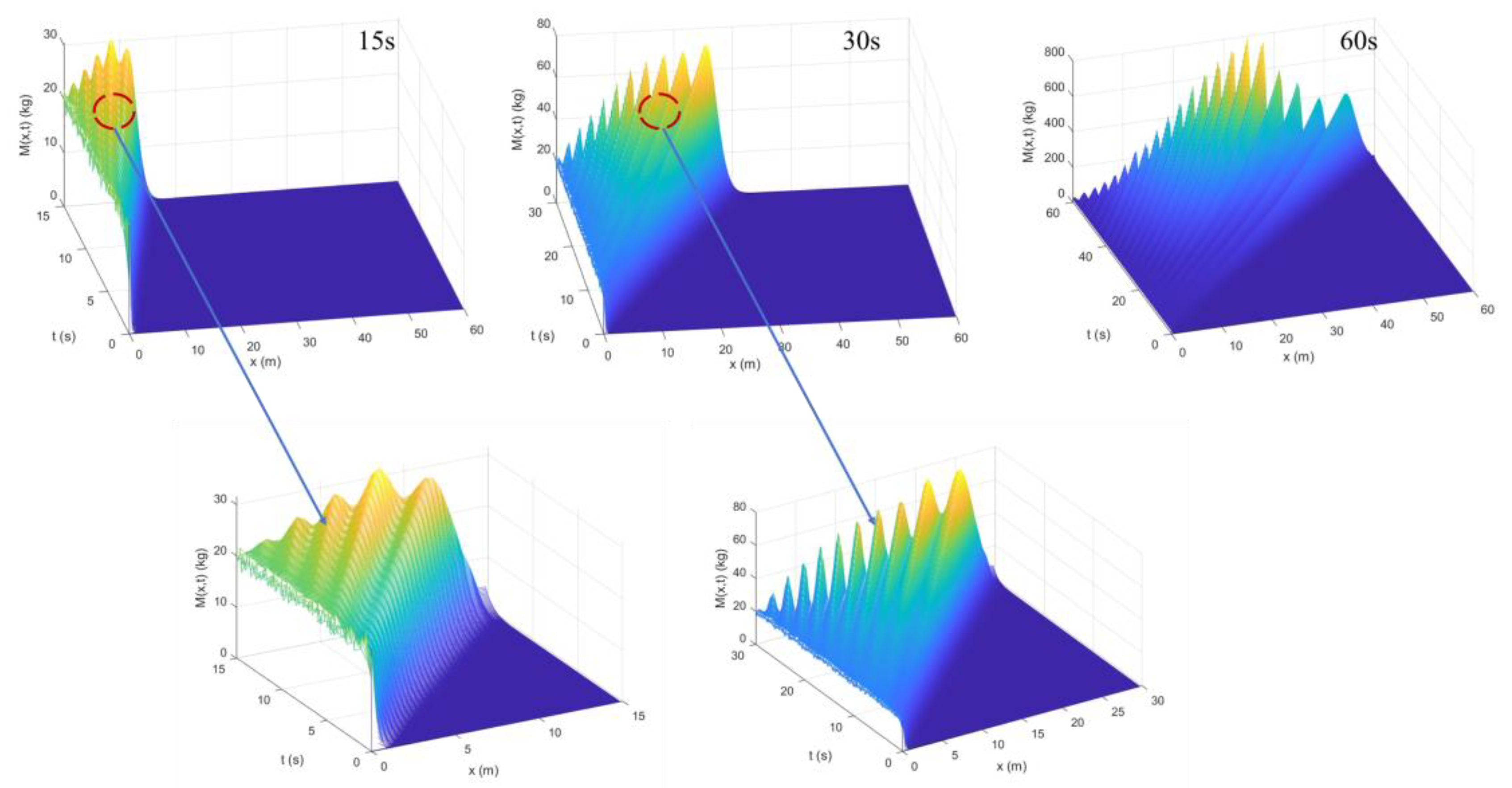
The Finite Difference Method (FDM) transforms partial differential equations into algebraic equations, enabling approximate solutions through iterative computation. By discretizing both time and space domains, FDM effectively addresses the computational challenges posed by coal flow variations. The overall solution process is illustrated in Figure 3.

Spatial discretization: The physical space is divided into evenly spaced nodes, with a spatial step size Δx. The coal mass at each node is calculated to simulate its spatial distribution. Time discretization: the time domain is divided into discrete time steps Δt, updating coal mass at each step.

By discretizing space and time, continuous PDEs are transformed into discrete difference equations, making them more suitable for numerical computation.

(2)

Solving the coal flow model using the finite difference method

From the previous analysis, the dynamic coal flow equation can be expressed as follows:

$${\displaystyle \frac{\partial M(x,t)}{\partial t}}+{\displaystyle \frac{\partial }{\partial x}}\left(v(x,t)\cdot M(x,t)\right)=(\alpha (x,t)-\beta (x,t))\cdot M(x,t)$$

(25)

The discretization process follows these steps:

(a) Spatial discretization:

The spatial domain is divided into multiple discrete points along the x-axis. The distance between two adjacent points is represented by the step size Δx. Each spatial position x_i is indexed as x_i = iΔx, M(x_i,t) is represented as M_iⁿ, where n is the time step index, indicating the coal mass at position x_i and time t_n = nΔ. The spatial derivative is approximated using either the central difference method or the forward difference method:

$${\displaystyle \frac{\partial }{\partial x}}\left(v(x,t)\cdot M(x,t)\right)\approx {\displaystyle \frac{(v_{i+1}^n{M}_{i+1}^n)-(v_i^n{M}_i^n)}{\Delta x}}$$

(26)

(b) Time Discretization:

The time axis is also divided into discrete steps with a step size of Δt. The time derivative is approximated using the finite difference method as follows:

$${\displaystyle \frac{\partial M(x_i,t_n)}{\partial t}}\approx {\displaystyle \frac{M_i^{n+1}-M_i^n}{\Delta t}}$$

(27)

By discretizing the revised equation and substituting the finite difference expressions, the difference equation is:

$${\displaystyle \frac{M_i^{n+1}-M_i^n}{\Delta t}}+{\displaystyle \frac{(v_{i+1}^n{M}_{i+1}^n)-(v_i^n{M}_i^n)}{\Delta x}}={\alpha }_i^n{M}_i^n-{\beta }_i^n{M}_i^n$$

(28)

Rearranging the difference equation to express M_iⁿ⁺¹ explicitly leads to the following:

$$M_i^{n+1}=M_i^n+\Delta t[-{\displaystyle \frac{(v_{i+1}^n{M}_{i+1}^n)-(v_i^n{M}_i^n)}{\Delta x}}+{\alpha }_i^n{M}_i^n-{\beta }_i^n{M}_i^n]$$

(29)

2.2. Dynamic Coal Flow Simulation Model Based on Discrete Element Method

2.2.1. Discrete Element Contact Model for Coal Particles

(1) Contact model theory

This study employs EDEM(2022) software for simulation modeling. EDEM is a widely used discrete element simulation platform for modeling the behavior of particulate and bulk materials. Due to its accuracy and flexibility in modeling particle contact behavior, it has been extensively applied in studies of coal mining and transportation processes, such as coal cutting, conveying, and unloading (Wang et al., 2024; Liu et al, 2018) [31,32]. Previous research has demonstrated that EDEM offers good applicability and reliability for simulating the dynamic behavior of coal flow in equipment such as scraper conveyors.

In EDEM, particle interactions are governed by multiple contact models, including the contact stiffness model, slip model, and bonding model. The contact stiffness model defines the relationship between force and displacement during particle collisions; the slip model describes tangential relative motion between particles; and the bonding model simulates particle adhesion or cohesion. These models together form the simulation foundation for accurately reproducing the behavior of coal particles in dynamic conveying processes, enabling realistic representation of coal flow within the scraper conveyor system.

Given that coal contains moisture, adhesion between particles is influenced by liquid bridge and van der Waals forces. The “Hertz-Mindlin with bonding” model is employed to simulate these interactions during the coal-cutting process. Coal and gangue particles interact via bonding forces that break under stress, after which the particles revert to elastic contact. For two colliding particles with velocities v_i,v_j and angular velocities x_i,x_j, the contact mechanics model is shown in Figure 4.

According to Hertz contact theory, the force and displacement of coal particles are:

$$F={\displaystyle \frac{4}{3}}{E}^{*}{(R^{*})}^{1/2}{\epsilon }^{3/2}$$

(30)

$$U={\left({\displaystyle \frac{3F{R}^{*}}{4E^{*}}}\right)}^{1/3}$$

(31)

$${\displaystyle \frac{1}{E^{*}}}={\displaystyle \frac{1-{\nu }_1^2}{E_1}}+{\displaystyle \frac{1-{\nu }_2^2}{E_2}}$$

(32)

where F represents the force between two coal particles, U is the relative displacement, E* is the equivalent elastic modulus, R* is the equivalent contact radius, and ε is the overlap between the particles.

The normal stiffness k_n, tangential stiffness k_s, normal force F_n, and tangential force F_s during the particle collision and breakage process are given by:

$$k_n={\displaystyle \frac{2E}{3(1-{\mu }^2)}}{(R^{*})}^{1/2}$$

(33)

$$k_s={\left({\displaystyle \frac{E}{1+\mu }}\right)}^{2/3}{\displaystyle \frac{(12(1-\mu )R^{*}{F}_n)1/3}{2-\mu }}$$

(34)

$$F_n=k_n{U}_n^{3/2}$$

(35)

$$F_s=k_s{U}_s^{3/2}$$

(36)

where E represents the elastic modulus of the coal particle, l is the Poisson’s ratio, U_n is the normal displacement, and U_s is the tangential displacement of the coal particle.

(2) Particle model and parameter settings

The selection of material parameters is crucial for contact force calculations and model solutions. The bonding strength of coal particles is based on their physical and mechanical properties. Studies by Abousleiman [33] and Xu et al. [34] provide the theoretical basis for the coal wall model. Experimental analysis of coal properties supports the calculation of normal and tangential stiffness for coal particles. Li et al. [35] also studied the effect of coal particle micro-parameters on bulk flow behavior and calibrated the parameters for both dry and wet coal. The accuracy of these parameters was verified through slide plate tests, and contact parameters such as the friction coefficient between coal and steel were determined. In the simulation, particle bonding parameters are set based on coal hardness and compressive strength, ensuring a compressive strength of 18 MPa with a Poisson’s ratio of 3. The material parameters are listed in

Table 1. Material parameters for coal and rock.

Parameter	Coal	Rock	Steel
Density (kg/m3)	1430	2600	7850
Shear Modulus (GPa)	0.38	3.3	70
Elastic Modulus (GPa)	0.99	8.14	190
Poisson’s Ratio	0.3	0.2	0.36
Particle Radius (10−2 m)	14	13	/
Bonding Radius (10−2 m)	15	14	/

and

Table 2. Particle bonding contact parameters.

Parameter	Coal-Coal	Coal-Rock	Coal-Steel
Static Friction Coefficient	0.329	0.35	0.46
Kinetic Friction Coefficient	0.036	0.034	0.032
Restitution Coefficient	0.53	0.56	0.65
Normal Stiffness (N/m3)	9.48 × 109	9.48 × 109	/
Tangential Stiffness (N/m3)	5.50 × 109	5.50 × 109	/
Normal Stress (Pa)	9.55 × 105	9.55 × 105	/
Tangential Stress (Pa)	3.21 × 106	3.21 × 106	/

.

The coal particle model in this study is built using spherical particles. While real coal particles are often hammer-shaped or blocky, spherical particles are used to simplify calculations and improve simulation efficiency. In EDEM software, a model of typical coal particle shapes is created, as shown in Figure 5.

2.2.2. Three-Dimensional Construction Model of Mining Equipment

In discrete element simulations, the geometric model is essential for accurately representing the equipment and the environment. For coal flow simulations, the modeling of the mining machine and scraper conveyor is critical. To reduce the computational load, the equipment geometry is simplified in this study. The scraper conveyor model includes key parts such as the scraper chain, frame, guide rails, and trough to accurately represent its effect on coal flow. The mining machine focuses on the cutting and traction sections to reflect its operation and interaction with the coal flow.

In EDEM, simple geometric shapes are created directly, while more complex ones are imported from AutoCAD 2020 models (e.g., Autodesk Inventor or SolidWorks 2022, saved as STL files) for better accuracy. Based on the parameters in

Table 3. Structural parameters of mining machine and scraper conveyor.

Type	Data	Type	Data
Mining machine model	MG500/1180-WD	Blade diameter	1400 mm
Scraper conveyor model	SGZ800	Blade helical angle	20°
Drum diameter	1800 mm	Blade rotation direction	Sequential
Drum hub diameter	1000 mm	Number of blade cutters	21
Drum width	1000 mm	Cutter layout	18
Cutting depth	800 mm	Number of blade heads	3
Middle trough dimensions	1500 × 800 × 303 mm	Chain specifications	34 × 126 mm

, the mining machine and scraper conveyor models are built in SolidWorks and imported into EDEM. The 3D models are shown in Figure 6.

2.2.3. Discrete Element Method Coal Flow Simulation Model Construction

After constructing the particle and geometric models, the mining machine, coal wall, and scraper conveyor models are integrated, forming the simulation model shown in Figure 7. In this model, coal particles that fall into the scraper conveyor’s middle trough are considered transported coal. As a result, all areas in the model, except the middle trough, are set as walls, with an additional wall at the top to block upward-moving coal particles, ensuring accurate simulation results.

Additionally, to validate the dynamic coal flow model, a virtual mass sensor is installed on the scraper conveyor to track and record coal mass changes in real time. The data from this sensor assist in theoretical analysis and model validation. The final simulation model is shown in Figure 8.

2.3. Dynamic Coal Flow Model Calculation and EDEM Simulation Analysis

2.3.1. Dynamic Coal Flow Theory Model

Based on the dynamic coal flow mathematical model and its numerical computation method, the following operating parameters were set: the shearer’s traction speed was 5 m/min, the drum rotation speed was 50 rpm, the cutting depth was 0.8 m, and the scraper conveyor chain speed was 60 m/min. The cutting duration was set to 60 s. Under these conditions, the dynamic coal flow model was used to calculate the spatiotemporal distribution of coal quantity on the scraper conveyor. To clearly observe this distribution, Figure 9 illustrates the coal distribution at 15 s, 30 s, and 60 s.

As shown in Figure 9, with the increase in cutting time, the coal quantity on the scraper conveyor changes continuously. This variation is mainly influenced by the operation mode of the shearer, the cutting rate, the traction speed, and the coal seam characteristics. Due to the continuous forward movement of the shearer, the coal flow accumulation and transportation processes are not uniform or steady. Instead, they exhibit dynamic fluctuation characteristics—coal quantity at different conveyor positions changes over time, resulting in a non-uniform spatiotemporal distribution.

To further analyze coal flow characteristics and quantitatively evaluate coal quantity changes at different locations, the coal flow distribution at 15 s was selected for detailed analysis. The spatial coal distribution data along the scraper conveyor at this time were extracted, and the total coal quantity over the 15 s period was also calculated. As shown in Figure 10, the red frame shows spatial variation, the black frame shows temporal variation, and the yellow frame shows total coal quantity changes.

2.3.2. Discrete Element Simulation Based on EDEM

After constructing the dynamic coal flow simulation model for the dual-machine system, the simulation parameters were set consistent with those of the mathematical model: shearer traction speed of 5.5 m/min, drum speed of 50 rpm, cutting depth of 0.8 m, and scraper chain speed of 60 m/min. The cutting time was set to 60 s. The EDEM software was used to carry out discrete element simulations, aiming to reproduce the dynamic coal transportation process.

As shown in Figure 11, the simulation results visually illustrate the evolution of coal blocks after being cut by the shearer and loaded onto the conveyor. The coal flow is not uniformly distributed, being influenced by the cutting rhythm, chain movement, and coal accumulation. This results in noticeable spatial fluctuations in coal distribution.

To analyze the coal distribution more precisely, data from virtual mass sensors in EDEM were extracted, as shown in Figure 12. The analysis focused on the coal distribution at the 7 m position of the conveyor, the instantaneous coal distribution at 7 s, and the cumulative coal quantity during the entire cutting process. These data reveal the spatiotemporal characteristics of the coal flow and provide theoretical support for coal transport optimization.

2.4. Model Validation and Comparative Analysis

To verify the consistency between the mathematical model and the simulation results, both line charts and boxplots were used to compare data trends and statistical characteristics. As shown in Figure 13, the line charts show that the temporal and spatial variation trends of the simulation data closely match those of the mathematical model. Peaks and valleys align well, indicating that the model accurately describes coal flow behavior. The boxplots show that both data sets have similar medians and interquartile ranges, suggesting that the model effectively captures coal flow fluctuation patterns. Together, these results confirm the model’s validity and reliability.

To further quantify the agreement, statistical evaluations including the Kolmogorov–Smirnov (K-S) test, Spearman’s correlation, Median Absolute Deviation (MAD), and Quantile Absolute Errors were conducted. The K-S test assesses whether the two data sets come from the same distribution, with a p-value above 0.05 indicating no significant difference. The Spearman correlation reflects consistency in trend, where a value near 1 indicates strong correlation. MAD measures overall deviation, while quantile errors assess accuracy at the 25%, 50%, and 75% percentiles. The detailed results of these statistical evaluations are presented in

Table 4. Statistical comparison between model and simulation results.

	K-S Test (p-Value)	Spearman (R)	MAD	Q25%	Q50%	Q75%
Total Coal Quantity	0.2176	0.9899	48.7993	27.229	42.601	45.229
Spatial Distribution	0.8253	0.9620	0.2652	0.007	0.192	0.321
Temporal Variation	0.4503	0.9662	2.5104	0.326	3.161	0.445

.

3. Mechanics and Energy Consumption Modeling of the Scraper Conveyor

3.1. Force Analysis and Mechanical Model of the Scraper Conveyor

The operating resistance of a scraper conveyor consists of two main components: resistance in straight sections and curved sections. In the straight sections, resistance mainly comes from friction on the load-bearing and non-load-bearing sides. The load-bearing side experiences resistance due to the material weight and friction between the material and scraper chain, while the non-load-bearing side is primarily affected by friction between the scraper chain and the base plate.

In curved sections, resistance is influenced by the bending of the scraper chain and system layout. Additional structural bending resistance occurs when the scraper chain passes around the drive sprocket, while operational bending resistance arises from uneven base plates and the movement of the conveyor structure. The classification of these loads is illustrated in Figure 14.

3.1.1. Resistance in Straight Sections

In the straight sections, the primary resistance comes from the frictional forces acting on both the load-bearing and non-load-bearing sides, generated by the interaction between the scraper chain and the base plate. Regardless of the load condition, frictional resistance opposes the chain’s movement.

(1) Resistance on the load-bearing and non-load-bearing chains

The scraper chain experiences resistance mainly due to friction with the base plate, which differs between the load-bearing and non-load-bearing sides [36]. As shown in Figure 15, during operation in straight sections, the scraper chain must overcome two key forces: the gravitational component along the inclined direction and frictional resistance. Both forces act against the chain’s movement, except when the chain moves downward, where gravity assists motion while frictional resistance remains opposing. The total resistance in straight sections can be expressed as follows:

$$T_{12}=q_{1}Lg\left(f\cos a\pm \sin a\right)$$

(37)

where q₁ represents the mass per unit length of the scraper chain (kg/m), L is the length of the straight section (m), α is the conveyor angle (positive when moving upward, negative otherwise), and f is the friction coefficient between the scraper chain and the chute bottom.

(2) Resistance from bulk material on the load-carrying side

On the load-carrying side, material exerts both vertical and lateral pressure on the chute. The lateral pressure increases resistance by enhancing friction with the sidewalls. The lateral pressure N is given by:

$$N=r{h}^2\lambda g$$

(38)

The scraper conveyor must overcome gravitational and frictional resistance from normal and lateral pressures, as expressed in:

$$T_3=L[g{q}_2(f_{1}cosa+sina)+f_{1}r{h}^2\lambda ](\alpha <{25}^{\circ })$$

(39)

where r is the weight per unit volume of the material, h is the height of the coal-retaining plate, λ is the material’s pressure coefficient on the sidewalls, and f₁ is the friction coefficient between the material and the chute.

In the empty section, the scraper chain moves along the bottom plate, with the main resistance coming from the friction between the chain and the plate. Therefore, the resistance in the empty section can be expressed as the total frictional resistance of the chain.

$$T_1=q_{1}Lg\left(f\cos a-\sin a\right)$$

(40)

In the loaded section, the scraper chain must overcome both its own frictional resistance and the additional resistance from moving the material. Thus, the total resistance is the sum of the chain’s friction and the material’s resistance:

$$T_4=q_{1}Lg\left(fcosa+sina\right)+L[g{q}_2(f_{1}cosa+sina)+f_{1}r{h}^2\lambda ](a<25°)$$

(41)

(3) Bending Resistance

(1) Operating Condition Bending Resistance

① Horizontal bending resistance

The scraper conveyor chute can bend both vertically and horizontally in its structure. However, in practical use, except for cases where the machine body moves, measures are typically taken to avoid horizontal curves. Figure 16 shows a schematic of the horizontal bending in the moving section of the machine body.

In a flexible scraper conveyor, the scraper chain follows a zigzag path in the bending section. When the friction coefficient between the chain and bottom plate is much higher than the equivalent friction, the resistance follows Euler’s formula. Thus, the frictional resistance in the bending section can be calculated using Euler’s formula for flexible bodies [37]:

$$S_1=S_y{\mathrm{e}}^{\mu {\alpha }^1}$$

(42)

where μ is the friction coefficient between the scraper chain and chute, a¹ is the angle between adjacent chutes, S₁ is the chain tension at the end of the previous chute, and n is the number of chutes in the bending section.

To simplify the analysis, the vertical bending resistance is typically neglected when calculating the tension in the horizontal bending section. Thus, the chain tension at the beginning of the first chute is given by Equation (43), and the tension at the end of the first chute is given by Equation (44). When the chain moves from position n to position n + 1, the required tension is given by Equation (45).

$$F_{11}=S_1.e^{\mu {\alpha }^{\prime }}$$

(43)

$$F_{12}=F_{11}+T_R=S_1{e}^{u{\alpha }^{\prime }}+T_C$$

(44)

$$\begin{array}{l}{F}_{(n+1)1}=F_{n2}{e}^{\mu {\alpha }^{\prime }}\\ =S_1{e}^{{(n+1)}^{\mu {\alpha }^{\prime }}}+T_C(e^{n\mu {\alpha }^{\prime }}+e^{{(n-1)}^{\mu {\alpha }^{\prime }}}+\dots e^{\mu {\alpha }^{\prime }})\\ =S_1{e}^{{(n+1)}^{\mu {\alpha }^{\prime }}}+T_C{\displaystyle \frac{e^{\mu \alpha \prime }(e^{n\mu \alpha \prime }-1)}{e^{\mu \alpha \prime }-1}}\end{array}$$

(45)

The variation in chain tension within the bending section is illustrated in Figure 17. Therefore, through reasoning, the additional resistance in the horizontal bending section is expressed by Equation (46).

$$\begin{array}{l}{F}_5=F_{(n+1)1}-S_1-n{T}_C\\ =S_1(e^{(n+1)\mu {\alpha }^{\prime }}-1)+T_C[{\displaystyle \frac{e^{\mu {\alpha }^{\prime }}(e^{n\mu {\alpha }^{\prime }}-1)}{e^{\mu {\alpha }^{\prime }}-1}}-n]\end{array}$$

(46)

② Vertical additional resistance

Vertical bending occurs when adjacent chutes rotate relative to each other due to an uneven conveyor bottom. The bending angle depends on the scraper conveyor structure and the bottom plate’s unevenness, as shown in Figure 18.

As shown in Figure 18, let S₀ be the chain tension at the end of the straight section. Upon entering the bending section, the tension gradually increases due to the deflection of the chute. The chain tension at the start of the first section of the bending section can be expressed as in Equation (47):

$$S_{11}=S_0\cdot {\mathrm{e}}^{{\mu }_{a_1}}$$

(47)

At the end of the first section of the bending section, the chain tension S₁₂ is increased by the resistance T_c of the straight section.

$$S_{12}=S_{11}+T_C=S_0.e^{\mu {\alpha }_1}+T_C$$

(48)

Based on the above recursive relationship, the general expression for the chain tension S_n2 at the end of the n-th section of the bending section is expressed as follows:

$$S_{n2}=S_0\cdot e^{\mu {\displaystyle \sum _{i=1}^n{\alpha }_i}}+T_C\cdot {\displaystyle \sum _{k=1}^n{e}^{\mu {\displaystyle \sum _{j=k}^n{\alpha }_j}}}j=2,3,\dots \dots ,n$$

(49)

For simplicity, the average deflection angle of the chute is used in place of the actual deflection angle. Therefore, S_n2 is given by Equation (47):

$$S_6=S_0\cdot {\mathrm{e}}^{\mu n\alpha }+T_C\cdot {\mathrm{e}}^{\mu \alpha }{\displaystyle \frac{{\mathrm{e}}^{n\mu \alpha }-1}{{\mathrm{e}}^{\mu \alpha }-1}}$$

(50)

Thus, the vertical bending additional resistance is given by Equation (51):

$$S_6=S_0({\mathrm{e}}^{\mu n\alpha }-1)+T_C({\mathrm{e}}^{\mu \alpha }{\displaystyle \frac{{\mathrm{e}}^{n\mu \alpha }-1}{{\mathrm{e}}^{\mu \alpha }-1}}-n)$$

(51)

where n is the number of chutes in the vertical bending section, and a is the average vertical deflection angle of each chute.

(2) Simplified horizontal and vertical additional resistance

① Empty return chain plate horizontal additional resistance

In flexible scraper conveyors, the chute deflection angle typically does not exceed 3°. For simplicity, small-angle bending resistance can be approximated as linear, allowing multiple small-angle bends to be treated as a single total bending angle α. The simplified horizontal bending of the moving section is shown in Figure 19.

The simplified horizontal additional resistance is given by Equation (52):

$$F_7=T({\mathrm{e}}^{f\alpha }-1)$$

(52)

$$T=S_1+q_{1}g{L}_1(f\cos a-\sin a)$$

(53)

$$\alpha =2\arcsin ({\displaystyle \frac{b\sin (\frac{{\alpha }^{\prime }}{2})}{\sqrt{2bl}}})$$

(54)

where l is the length of each chute section, α′ is the angle between adjacent chutes, b is the moving step size, and L₁ is the distance from the conveyor head to the horizontal bending point.

② Horizontal additional resistance of the load-bearing chain plate

When the chain runs in the same direction as the mining direction, horizontal resistance occurs at the contact between the load-bearing chain plate and the chute sidewalls in the bending section. If the direction is opposite, additional coal transportation tension from the tail to point A is included in the tension calculation. When the chain direction aligns with the mining direction, the following is observed:

$${\mathrm{F}}_8{ =(\mathrm{T}}_l+{\mathrm{S}}_3)\times ({\mathrm{e}}^{2\alpha f}-1)$$

(55)

$${\mathrm{S}}_3{ =\mathrm{K}}_2({\mathrm{S}}_1+F_7+T_2)$$

(56)

where L is the length of the scraper conveyor, L₃ is the vertical distance in the horizontal bending section, and K₂ is the resistance coefficient of the tail wheel axle.

③ Vertical bending additional resistance

For a simplified calculation, the vertical bending resistance is proportional to the total sum of the absolute bending angles. An equivalent bending angle can be used to simplify the calculation. The simplified diagram is shown in Figure 20.

The vertical bending resistance for both the loaded and unloaded branches is expressed as follows:

$${\mathrm{F}}_9={\mathrm{S}}_1({\mathrm{e}}^{f\beta }-1)$$

(57)

$${\mathrm{F}}_{10}={\mathrm{S}}_3({\mathrm{e}}^{f\beta }-1)$$

(58)

3.1.2. Structural Bending Additional Resistance

In addition to the aforementioned additional resistances, the bending of the scraper chain at the sprocket and the rotation of the sprocket bearings also generate additional resistance, as shown in Figure 21:

When the return pulley is positioned in the empty branch, the scraper chain passes over the return pulley without carrying material, and the resistance is given by Equation (59). In contrast, when the return pulley is positioned in the loaded branch, the resistance is given by Equation (60)

$${\mathrm{T}}_5=2S_2(\mu \sin {\displaystyle \frac{{\alpha }_1}{2}}\cdot {\displaystyle \frac{\mathrm{d}}{\mathrm{D}}})$$

(59)

$${\mathrm{T}}_6=2S_2(\mu \sin {\displaystyle \frac{{\alpha }_1}{2}}\times {\displaystyle \frac{\mathrm{d}}{\mathrm{D}}})+{\mathrm{R}}_1{\alpha }_1{\mathrm{x}[\mathrm{G}}_0(\sin {\displaystyle \frac{{\alpha }_1}{2}}+f_1{\displaystyle \frac{{\alpha }_1}{2}})+f_{1}r{h}^{2}t\lambda ]$$

(60)

where D is the return wheel diameter, a₁ is the wrap angle of the scraper chain on the return wheel in radians, d is the chain return diameter, and u is the friction coefficient of the scraper chain.

3.2. Energy Consumption Model for the Scraper Conveyor

In mining operations, the scraper conveyor operates in two conditions: when the scraper chain moves in the same direction as the mining machine and when they move in opposite directions. Figure 22 shows the case of reverse operation with dual machines. In the same-direction operation, compared to the reverse operation, only the coal transport tension from point A to the mining machine needs to be increased, while the forces on the scraper chain and the coal flow characteristics remain unchanged.

(1) Straight-line resistance

$$\begin{array}{l}{T}_h=\{q_{1}Lg\left(fcosa-sina\right)+q_{1}Lg\left(fcosa+sina\right)+\\ \hspace{1em}\hspace{1em}\hspace{1em}(L_1+L_2)[g{q}_2(f_{1}cosa+sina)+f_{1}r{h}^2\lambda ]\}\end{array}$$

(61)

(2) Horizontal bending resistance

$$\begin{array}{l}{F}_h=[(S_1+q_{1}g{L}_1(fcosa-sina))({\mathrm{e}}^{2f\alpha }-1)]+[(q_1(\mathrm{L}-{\mathrm{L}}_1-{\mathrm{L}}_3)g\left(fcosa+sina\right)+\\ { \mathrm{K}}_2({\mathrm{S}}_1+(S_1+q_{1}g{L}_1(fcosa-sina))({\mathrm{e}}^{2f\alpha }-1))+q_{1}Lg\left(fcosa-sina\right))\times ({\mathrm{e}}^{2\alpha f}-1)\end{array}$$

(62)

(3) Vertical bending resistance

$$\begin{array}{l}{\mathrm{F}}_v=(S_1+({\mathrm{K}}_2\times ({\mathrm{S}}_1+(S_1+q_{1}g{L}_1(fcosa-sina))\times ({\mathrm{e}}^{2f\alpha }-1)\\ \hspace{1em}\hspace{1em}\hspace{1em}\hspace{1em}\hspace{1em}\hspace{1em}\hspace{1em}+q_{1}Lg(fcosa-sina))))\times ({\mathrm{e}}^{f\rho }-1)\end{array}$$

(63)

(4) Resistance due to the scraper chain passing the return wheel

$${\mathrm{T}}_z=4S_2(\mu \sin {\displaystyle \frac{{\alpha }_1}{2}}\cdot {\displaystyle \frac{\mathrm{d}}{\mathrm{D}}}+{\mu }_1{\displaystyle \frac{{\mathrm{d}}_1}{\mathrm{D}}})+{\mathrm{R}}_1{\alpha }_1\mathrm{x}[{\mathrm{G}}_0(\sin {\displaystyle \frac{{\alpha }_1}{2}}+f_1{\displaystyle \frac{{\alpha }_1}{2}})+f_{1}r{h}^2\lambda ]$$

(64)

(5) Total resistance of the scraper conveyor

$$F_z=T_h+F_h+F_v+T_z$$

(65)

(6) Power consumption

$$P={\displaystyle \frac{V_j\times F_Z\times k_j}{{\eta }_j}}$$

(66)

where k is the motor spare power coefficient, and η is the overall efficiency of the transmission system. Thus, the energy consumption of the scraper conveyor is:

$$W={\displaystyle \underset{t0}{\overset{t1}{\int }}p(t)dt}$$

(67)

3.3. Speed Coordination Optimization Model

3.3.1. Optimization Variables

In the ideal case, once the characteristics of the mining face and the models of the mining machine and scraper conveyor are determined, the energy consumption of the dual-machine system depends mainly on the traction speed, drum speed, and scraper chain speed. Therefore, the optimization variables are the traction speed, drum speed, and scraper chain speed at each stage of operation.

$$X={(v_q,v_j,n)}^T=(x_1,x_2,x_3)$$

(68)

3.3.2. Optimization Objective

This study focuses on the impact of coal flow variation on the energy consumption of the scraper conveyor. The optimization objectives are the lump coal area and scraper conveyor energy consumption. Coal flow fluctuations are mainly influenced by coal lump size distribution. During transportation, large coal lumps should be avoided while ensuring that the lump size remains within a medium-to-small range to meet optimal specifications. Therefore, the optimization goal is to adjust the lump coal size distribution to improve transportation efficiency and reduce energy consumption.

The coal lump size range of 50 mm to 100 mm is chosen as the preferred range. This size range is between medium and large lumps, which can reduce the load on the scraper conveyor while maintaining a high lump coal rate. Compared to lumps larger than 100 mm, lumps in the 50 mm to 100 mm range can reduce equipment wear, clogging risks, and energy loss during transportation.

Based on the cutting mechanism of the cutter teeth, as shown in the cutting diagram in Figure 23, the larger the cutting area, the larger the lump size and the higher the lump coal rate. Thus, the lump coal area is an important parameter for evaluating lump size. In the optimization process, converting lump coal size into lump coal area helps better quantify and control coal flow characteristics. When the lump coal size is between 50 mm and 100 mm, the corresponding lump coal area should range from 2500 mm² to 10,000 mm². By considering economic benefits, equipment load, and energy consumption, a lump coal area of 2500 mm² is chosen. This solution balances transportation efficiency and energy consumption, providing an optimal approach that is both economical and practical.

$$\left\{\begin{array}{l}H={\displaystyle \frac{1000v}{n}}\\ h_{max}={\displaystyle \frac{H}{N-1}}\\ h_2={\displaystyle \frac{H}{\pi D_C}}({\displaystyle \frac{\pi D_c}{N}}-{\displaystyle \frac{t}{\tan \phi }})\\ t={\displaystyle \frac{h_{max}}{N\left[\frac{1}{\tan \phi }-\frac{(N-1)h_{max}}{\pi D_C\tan \phi }\right]}}\end{array}\right.$$

(69)

$$S_a=(t/\sin \phi +0.5(h_2-t/\tan \varphi )/\cos \varphi )\times (N-1)t/\sin \varphi \times \sin 2\varphi$$

(70)

where H₂ is the maximum feed rate per revolution between cutter 2 and cutter 3, N is the number of spiral blade heads, D is the diameter of the roller, p is the angle of the spiral pitch, t is the cutting line distance, and φ is the coal’s collapse angle.

Therefore, considering both the coal block area and energy consumption, the following multi-objective grinding function is established:

$$\min F(X)=\left\{\begin{array}{l}{f}_1(x)={(S_a(x)-2500)}^2\\ f_2(x)=W(x)\end{array}\right.$$

(71)

3.3.3. Constraints

During the coal mining and transportation process, the drum speed, traction speed, and scraper conveyor speed need to remain within a reasonable range. Meanwhile, the coal mining and transportation time and coal quantity should be within the specified range. The coal mining and transportation time should not exceed the transfer task running time required by the production department, and the coal quantity should meet the production plan requirements. In addition, the block coal area must also satisfy certain constraints to ensure that the coal block size is within the optimized range. Therefore, the constraints of the optimization model can be expressed as follows:

$$st=\left\{\begin{array}{l}{h}_1(v_q,n)=t\le T^{goal}\\ h_2(v_q)=\{v_{q\min }-v_q\le 0;v_q-v_{q\max }\le 0\}\\ h_3(n)=\{n_{\min }-n\le 0;n-n_{\max }\le 0\}\\ h_4(v_j)=\{v_{j\min }-v_j\le 0;v_j-v_{j\max }\le 0\}\\ h_5(v_q,n)=Q\ge Q^{goal}\\ h_6(v_j,v_q,n)=2500\le S_a\le 10000\end{array}\right.$$

(72)

4. Adaptive Crossover Operator-Based Multi-Objective Binary Genetic Algorithm

Pan et al. [38] introduced a multi-objective genetic optimization algorithm that combines adaptive real-number encoding with simulated binary crossover rotation. The key idea is to use a rotation matrix V, derived from the covariance matrix of the current population, to rotate the solutions in the decision space. This, along with an adaptive operator selection strategy, aims to improve performance across various multi-objective optimization tasks. The process of the proposed NSGA-II-ARSBX is as detailed below.

4.1. Rotation-Based Simulated Binary Crossover

In this method, all parent solutions are rotated into a space aligned with the decision variables. Then, simulated binary crossover (SBX) is used to generate offspring solutions. Afterward, an inverse rotation is applied to bring the offspring solutions closer to their original parent solutions. Specifically, during the reproduction phase, the average vector m and the covariance matrix C for the population are calculated. The average vector m is calculated as follows:

$$m={\displaystyle \frac{1}{N}}{\displaystyle \sum _{i=1}^N{x}_i}$$

(73)

$$C_{ij}={\displaystyle \frac{{\displaystyle \sum _{k=1}^D(x_{i,k}-m_k)(x_{j,k}-m_k)}}{N-1}}$$

(74)

where x_ik and m_k are the k-th components of the i-th individual and the average vector m, respectively. Eigenvalue decomposition is then performed to obtain the eigenvector corresponding to the largest eigenvalue. The time complexity for this step is O(D3), where D is the number of decision variables. Using the rotation matrix R, the population is rotated, and SBX is applied to generate offspring solutions. Finally, the offspring solutions are rotated back to their original direction using the inverse matrix.

$$x_{offspring}=R^{-1}{x}_{generated}$$

(75)

4.2. Adaptive Operator Selection

In this study, a probability parameter p_s is introduced to select the crossover operator for offspring generation. Specifically, SBX is used with probability p_s and RSBX with probability 1 − p_s, and p_s is updated at each generation. Initially set to 0.5, it assumes that SBX and RSBX have an equal ability to generate high-quality offspring solutions. The calculation of p_s is as follows:

$$p_s={\displaystyle \frac{1}{1+exp(-kr)}}$$

(76)

$$r=({\displaystyle \frac{N_0^{(g)}+1}{N_r^{(g)}+N_0^{(g)}+2}}-0.5)*{\displaystyle \frac{g}{g_{max}}}$$

(77)

where k is set to a specific value, and p_s is defined as an S-shaped function ranging from 0 to 1. Additionally, the number of offspring solutions generated by SBX/RSBX and surviving from generation g is denoted as rNog. This parameter helps introduce problem complexity to determine the likelihood of using SBX with p_s. The complexity of the problem is typically related to the number of objectives M and decision variables D, and thus both parameters are utilized. Since D is usually much larger than M, the square root of D and M is used to balance these factors.

The flow of the NSGA-II + ARSBX algorithm is shown in Figure 24, with the main steps as follows:

(1) Initialization of population

Randomly generate the initial population and calculate objective values as fitness. Initialize ARSBX parameters (rotation matrix, mean vector m, crossover probability, distribution index, etc.).

(2) Non-dominated sorting

Sort the population based on objective values using Pareto dominance, assigning Pareto ranks to solutions. Lower ranks indicate higher-quality solutions.

(3) Crowding distance calculation

For each Pareto level, compute the crowding distance to measure solution distribution in the objective space. Larger distances help maintain diversity.

(4) Selection operation

Select N parents based on Pareto rank and crowding distance, prioritizing low-rank and large-distance solutions for quality and diversity.

(5) Adaptive ARSBX crossover and mutation operations

ARSBX crossover: Generate offspring using ARSBX, dynamically adjusting parameters based on population distribution. Perform crossover in the rotated space and reverse transform to the original space. Adjust crossover probability and distribution index η based on the evolution stage.

Mutation: apply adaptive mutation to offspring to enhance diversity, with mutation probability adjusting during evolution.

(6) Population update

Merge the current population with offspring, then perform non-dominated sorting and crowding distance calculation. Select the top N solutions for the next generation.

(7) ARSBX parameter update

Update ARSBX parameters (rotation matrix V mean vector m, crossover probability p, and distribution index η) based on population distribution or fitness feedback.

(8) Repetition of iteration

Repeat steps 2–7 until the maximum generations g_max are reached or the termination criteria are met.

(9) Output results

Output the non-dominated solutions from the final population as the Pareto front and record ARSBX parameter changes for optimization analysis.

5. Case Study and Validation

5.1. Experimental Background

A case study and experimental validation were carried out based on a fully mechanized working face at Yuan Datang Coal Mine. The working face is equipped with a comprehensive data acquisition and integration system, which is used to validate the shearer energy consumption model and the scraper conveyor energy optimization strategy based on the dynamic coal flow proposed in this study. As shown in Figure 25, the system includes (a) the overall layout of supporting equipment at the mining face, such as the shearer, hydraulic supports, and scraper conveyor; (b) a coal-flow-monitoring system installed along the scraper conveyor, utilizing 3D cameras and sensors to capture real-time coal flow profiles; (c) a shearer data acquisition module that records traction speed, drum rotation speed, and motor parameters including voltage and torque; and (d) a scraper conveyor data acquisition system that monitors chain speed, motor current, and load status for energy consumption analysis. The working face is equipped with an MG2×250/1200-WD shearer manufactured by China Coal Technology & Engineering Group Shanghai Co., Ltd., located in Shanghai, China, and an SGZ1000/3×1000 scraper conveyor produced by SANY Heavy Industry, based in Zhangjiakou, China.Their layout and main parameters are listed in

Table 5. Main technical parameters of shearer and scraper conveyor.

Parameter	Value	Parameter	Value
Production capacity	2000 t/h	Conveyor length	300–350 m
Cutting height range	1.3–3 m	Trough specification	1750 × 1000 × 370 mm
Production capacity	680/320 kN	Round link chain specification	48 × 152
Cutting height range	0~30.4 m/min	Rated voltage (conveyor)	3300 V
Shearer traction force	43 t	Rated current (conveyor)	196.7 A
Shearer main body weight	0–53.6 r/min	Rated current (cutting motor)	53 A
Rated power (cutting motor)	90 kw	Rated current (traction motor)	169 A
Rated voltage (cutting motor)	3300 V	Rated voltage (traction motor)	380 V

and

Table 6. Working face parameters.

Parameter	Values	Parameter	Values
Longwall length (L/m)	340	Cutting depth (H/m)	0.8
Triangle coal length (L3/m)	50	Coal seam dip angle (a3)	6
Tecovery rate (c/°)	0.98	Mining height (B/m)	3.3

, respectively. Accordingly, this section focuses on the dual-machine system and conducts simulation analysis and validation based on the scraper conveyor energy consumption model developed in Section 3.2.

Specifically, key parameters from actual operating conditions—such as the shearer’s traction speed, drum rotation speed, and the scraper conveyor speed—are input into the coal flow mathematical models established in Section 2 and Section 3 to calculate the theoretical coal flow data. These results are then compared with actual coal flow data collected by the monitoring system of the working face (see Figure 25b), corresponding to the “Original value”.This comparative analysis provides empirical validation for the proposed integrated coal flow modeling and energy optimization framework, further demonstrating its engineering applicability and predictive accuracy.

5.2. Optimization Simulation and Results

5.2.1. Simulation Parameters

The simulation and computation were performed on the MATLAB 2022b platform. The NSGA-II-ARSBX algorithm was used to solve the scraper conveyor energy consumption optimization model, with the initial parameters provided in

Table 7. NSGAII-ARSBX parameters.

Parameter	Values
Population size	100
Number of generations	200
Crossover probability	0.9
Mutation probability	0.1
Probability parameter	0.5
Crossover distribution index	10
Mutation distribution index	20
Number of iterations	500

. In addition, all simulation experiments in this study were conducted on a Think series personal computer configured with Windows 11 Professional 64-bit operating system, Intel(R) Core(TM) i5-8250U processor, and 8.00 GB RAM.

5.2.2. Simulation Results and Analysis

The optimization of the scraper conveyor energy consumption model was performed, and the Pareto front solutions are shown in Figure 26. As seen in the figure, the optimization objectives typically exhibit conflict and incommensurability, meaning that there is no single feasible solution that satisfies all objectives simultaneously (such as minimizing energy consumption and minimizing the coal block area). However, in practical applications, decision-makers often need to choose the optimal operating conditions based on specific goals. Therefore, this study introduces the Ideal Point Method to evaluate the Pareto front. In each set of optimal solutions, there is typically a trade-off relationship between the two conflicting objective functions. The research suggests that the closer the design point is to the ideal point, the better its overall performance [39]. Since the objective values in the figure are unevenly distributed, direct numerical comparison is not appropriate. Sayyaadi and Nejatolahi [40] proposed that the actual values can be replaced by a normalized Pareto front for analysis, which makes the objectives comparable. Therefore, the optimization objectives were normalized to make energy consumption and coal block area comparable. The normalized expressions for the objective functions E and Sa are as follows:

$$E={\displaystyle \frac{E-E_{min}}{E_{max}-E_{min}}}$$

(78)

$$S_a={\displaystyle \frac{S_a-S_{amin}}{S_{amax}-S_{amin}}}$$

(79)

E_max and E_min denote the maximum and minimum values of the objective function along the horizontal axis of the Pareto front, respectively. Similarly, S_amax and S_amin represent the maximum and minimum values of the objective function along the vertical axis of the Pareto front. The goal of this study is to achieve a balance between energy consumption and lump coal area. Therefore, the ideal point aims to minimize both energy consumption and lump coal area simultaneously. However, it is important to note that this ideal point does not lie on the Pareto boundary.

As shown in Figure 27, the ideal point is marked as point P. Point B, which is closest to the ideal point on the Pareto front, is defined as the optimal compromise solution on the Pareto boundary. Point B represents a solution that strikes a reasonable balance among multiple optimization objectives. After normalizing the Pareto front, an ideal optimal point p(E_i,Sa_i) can be determined based on specific optimization targets. In this study, the coordinates of the ideal optimal point are (E_min,S_amin).

The Euclidean distance from a Pareto front point to the ideal optimal point is defined as follows:

$$d=\sqrt{{(E-E_i)}^2+{(S_a-S_{ai})}^2}$$

(80)

Figure 27 presents the Pareto front scatter plot, illustrating the relationship between coal block area and energy consumption. According to the Ideal Optimal Point Method, Point B is identified as the closest solution on the Pareto front to the ideal point. At this point, the coal block area is 4912 mm² and energy consumption is 1.2617 × 10⁹ KJ. The corresponding optimized decision variables are as follows: shearer traction speed v_q = 6.1 m/min, scraper conveyor chain speed v_j = 31 m/min, and drum rotation speed n = 50 r/min. The optimized objective values for energy consumption E and coal block area S_a are 1.2617 × 10⁹ KJ and 4912 mm², respectively.

Further experimental validation is provided in

Table 8. Comparison of variables and objectives before and after optimization.

Optimization Type	Optimization Variable			Optimization Objective
	Vq (m/min)	Vj (m/min)	n (r/min)	E (KJ)	Sa (mm2)
B/min (E,Sa)	6.1	31	50	1.2617 × 109	4912
C/min (E)	7	30	41.6	1.0169 × 109	9989
A/min (Sa)	4.5	32	49.8	1.8086 × 109	2500
Original value	6	40	35	1.9034 × 109	13,827

“Original value” refers to the data before optimization, and “min(E,S_a)” represents the data before optimization.

, which presents a comparative analysis of the pre- and post-optimization results.

To evaluate the effectiveness of the proposed optimization strategy, a comparison is first made between the original working condition and the selected compromise solution (Point B). Under the original parameters, the system exhibits an energy consumption of 1.9034 × 10⁹ KJ and a lump coal area of 13,827 mm². After applying multi-objective optimization, Point B achieves an energy consumption of 1.2617 × 10⁹ KJ and a lump coal area of 4912 mm², representing a 33.7% reduction in energy consumption and a 64.5% reduction in lump coal area.

It should be noted that although a reduction in lump coal area is often associated with increased fragmentation, in this context, the decrease is intentional and beneficial. The optimization aims to avoid excessive formation of large lump coal, which may hinder conveying and processing efficiency. Therefore, the reduced lump coal area reflects a controlled refinement of coal structure rather than a decline in coal quality.

Compared with the single-objective optimization results—Point C (minimum energy: 1.0169 × 10⁹ KJ, but higher lump coal area: 9989 mm²) and Point A (minimum lump coal area: 2500 mm², but high energy: 1.8086 × 10⁹ KJ)—Point B (*) provides a balanced trade-off between energy efficiency and coal fragmentation. It avoids the extremes of excessive fragmentation or oversized coal blocks, and thus represents a practical and effective compromise for real mining operations, aligning energy-saving goals with acceptable coal integrity.

5.3. Correlation Parameter Analysis

To analyze the impact of decision variables on the objective functions, we used Response Surface Methodology (RSM). Common design methods include Central Composite Design (CCD) and Box–Behnken Design (BBD). BBD is especially suitable for estimating second-order response surfaces in experimental studies. Unlike CCD, which uses extreme factor levels, BBD carefully selects points at the center and midpoints of the experimental space, avoiding extreme combinations. This design reduces the number of experiments and minimizes the risk of failure due to extreme factor settings while ensuring model accuracy. In comparison to CCD’s axial point design, BBD does not require additional axial points. This makes it more efficient, especially when there are many factors, as it significantly reduces the number of experiments needed. Therefore, BBD was chosen in this study to assess the impact of three variables on the objective functions. Based on the BBD principles, 13 experimental runs were carried out. The factor levels and experimental plan are shown in

Table 9. Factor level coding.

Level	Vq (m/min)	Vj (mm)	n (r/min)
−1	2	30	20
0	4.5	65	30
1	7	100	50

and

Table 10. BBD experimental matrix with objective function values.

Run	Vq	Vj	n	Sa	E (×109)
1	2	30	40	5700.43	4.17477
2	7	30	40	15,983.1	1.06096
3	2	100	40	5700.43	13.0266
4	7	100	40	15,983.1	3.21057
5	2	65	30	6282.62	8.09433
6	7	65	30	27,460.8	2.06738
7	2	65	50	5440.57	9.09712
8	7	65	50	11,518.1	2.19038
9	4.5	30	30	12,641.3	1.60108
10	4.5	100	30	12,641.3	5.00289
11	4.5	30	50	7440.23	1.76725
12	4.5	100	50	7440.23	5.3341
13	4.5	65	40	8981.45	3.42053

.

To evaluate the effect of each variable, regression models were analyzed using an analysis of variance (ANOVA). A p-value of less than 0.05 indicates that the variable significantly affects the objective function. The smaller the p-value, the greater the influence of the variable. If the p-value is large, the variable has a negligible effect on the objective.

To clearly illustrate the different impacts of chain speed, traction speed, and drum speed on the objectives, an ANOVA was performed on the regression models of each variable. In this analysis, a p-value (p) less than 0.05 indicates that the parameter has a statistically significant effect on the objective. The smaller the p-value, the greater the significance of the variable’s impact on the objective. Conversely, larger p-values suggest that the parameter has a negligible effect on the objective.

From

Table 11. Energy consumption analysis of variance.

Source	Sum of Squares	Degrees of Freedom	Mean Squared Error	F-Value	p-Value Prob > Value	Importance
Model	7.048 × 109	9	7.831 × 108	117.41	0.0012
A (Vq)	4.167 × 109	1	4.167 × 109	624.79	0.0001	1 *
B (Vj)	2.289 × 109	1	2.289 × 109	343.19	0.0003	2 *
C (n)	1.532 × 107	1	1.532 × 107	2.30	0.2268	3 *
AB	1.617 × 108	1	1.617 × 108	24.24	0.0161
AC	4.156 × 106	1	4.156 × 106	0.62	0.4875
BC	19,407.67	1	19,407.67	2.910 × 10−3	0.9604
A2	2.632 × 108	1	2.632 × 108	39.45	0.0081
B2	1.126 × 107	1	1.126 × 107	1.69	0.2846
C2	81,802.20	1	81,802.20	0.012	0.9188
Residual	2.001 × 107	3	6.670 × 106	/	/
Cor Total	7.068 × 109	12	/	/	/

“p < 0.05” indicates a significant effect, marked with *, and the larger the value, the more important the effect.

, it is evident that the traction speed of the mining machine and the scraper chain speed are key factors influencing the energy consumption of the scraper conveyor. These factors directly affect the coal flow rate, the dynamic load, and system efficiency. Firstly, the traction speed of the mining machine determines the rate and volume of coal entering the scraper conveyor. As the traction speed increases, more coal is transported per unit of time, causing the scraper conveyor to overcome greater resistance and resulting in higher energy consumption. Additionally, fluctuations in traction speed can lead to frequent starts, stops, and accelerations. During these phases, the motor must handle higher currents to overcome inertia and coal flow resistance, further increasing energy consumption. Secondly, the scraper chain speed plays a significant role in coal transport efficiency and friction losses. An increase in chain speed leads to greater friction between the coal and the conveyor trough, raising operating resistance and consequently increasing motor energy consumption and chain wear. Improper chain speeds may cause coal accumulation, idling, or overload conditions, further increasing energy consumption and reducing efficiency. Moreover, the mining machine’s drum speed indirectly affects the conveyor system by influencing the fragmentation and uniformity of the coal flow. In conclusion, the traction speed of the mining machine and the scraper chain speed are critical factors in the analysis and optimization of scraper conveyor energy consumption as they directly influence coal flow rate and transport efficiency.

From

Table 12. Lump coal area analysis of variance.

Source	Sum of Squares	Degrees of Freedom	Mean Squared Error	F-Value	p-Value Prob > Value	Importance
Model	8541.10	6	1423.52	38.30	0.0002
A(Vq)	6152.65	1	6152.65	165.54	<0.0001	1 *
B(Vj)	0.000	1	0.000	0.000	1.0000	3
C(n)	1689.16	1	1689.16	45.45	0.0005	2 *
AB	0.000	1	0.000	0.000	1.0000
AC	699.28	1	699.28	18.81	0.0049
BC	0.000	1	0.000	0.000	1.0000
Residual	223.00	6	37.17	/	/
Cor Total	8764.10	12	/	/	/

“p < 0.05” indicates a significant effect, marked with *, and the larger the value, the more important the effect.

, it is clear that the mining machine’s traction speed and drum speed significantly affect the lump coal rate. The traction speed determines how fast the drum moves through the coal seam. A higher traction speed increases the impact and shear forces during cutting, leading to more coal fragmentation and a lower lump coal rate. Conversely, lowering the traction speed reduces coal breakage and improves the lump coal rate. The drum speed also plays a key role by controlling the frequency of the picks’ cutting and the evenness of coal fragmentation. A higher drum speed causes more frequent forces on the coal, producing smaller coal pieces and lowering the lump coal rate. A slower drum speed allows for more even cutting, helping the coal break more cleanly and increasing the lump coal rate. In contrast, the scraper chain speed mainly affects the coal flow during transport and has less of an impact on coal fragmentation. Regardless of whether the chain speed is fast or slow, it does not significantly change the coal flow pattern during transport, and thus does not notably affect the lump coal rate.

In addition, three-dimensional surface plots (Figure 28) were generated to clearly show the specific impacts of each parameter on the optimization objectives. Each set of plots involves two key variables related to a single optimization objective. An in-depth analysis of Figure 28 leads to the following key findings:

On one hand, as the traction speed decreases, while the scraper chain speed and drum speed increase, the energy consumption of the scraper conveyor rises significantly. Conversely, if the traction speed increases while the scraper chain speed and drum speed decrease, the energy consumption of the scraper conveyor decreases significantly. On the other hand, if the traction speed continues to increase and the drum speed also increases accordingly, the lump coal rate will improve significantly. In contrast, if the traction speed decreases and the drum speed also decreases, the lump coal rate will decrease accordingly.

In conclusion, selecting the optimal combination of variables based on actual production conditions is crucial. This approach not only ensures the achievement of expected production outcomes but also maximizes the efficient use of energy and successfully reduces production costs.

5.4. Practical Implications and Research Advancements

This study proposes a systematic approach to coal flow modeling and energy efficiency optimization for scraper conveyors, with the following contributions:

(1) To address the limitations of traditional static coal flow models and their inadequate description of spatial and temporal variations in coal quantity, this study develops a dynamic coal flow mathematical model based on the law of mass conservation. Accumulation and dissipation factors are incorporated to more accurately capture the dynamic changes in coal flow. The model is numerically solved using the Finite Difference Method (FDM), which offers high computational efficiency and strong applicability. Additionally, a 3D dynamic simulation considering particle contact mechanics and equipment motion is established using the EDEM discrete element method, revealing the relationship between coal flow fluctuations and energy consumption. The accuracy and practical applicability of the model are validated by comparing the mathematical model results with simulation data.

(2) The energy consumption structure and transmission characteristics of the scraper conveyor are systematically analyzed, focusing on the main sources of resistance, including resistance in straight sections, curved sections, and additional resistance when passing over return wheels. Based on this analysis, a detailed energy consumption mathematical model is established. The effects of three key parameters—traction speed, drum rotational speed, and chain speed—on energy consumption are quantitatively evaluated, clearly identifying traction speed and chain speed as the primary factors influencing the conveyor’s energy efficiency. The results demonstrate that by properly coordinating the speeds of the shearer and scraper conveyor, coal transport efficiency can be maintained while significantly reducing energy consumption and effectively minimizing the formation of large coal lumps.

(3) Conventional research predominantly addresses single-equipment or singular optimization objectives, often overlooking the coupled impact on both energy consumption and lump coal size. This study implements a multi-objective optimization framework that simultaneously targets these two critical factors. Utilizing the NSGA-II algorithm augmented with adaptive simulated binary crossover (ARSBX), the approach enhances both solution diversity and convergence efficiency. The resulting compromise solutions effectively balance energy efficiency with lump coal size, demonstrating considerable practical applicability and providing valuable insights for engineering decision-making.

6. Conclusions

This study focuses on optimizing the energy efficiency of coal mining equipment, with a primary focus on developing dynamic coal flow and scraper conveyor energy efficiency models. The effects of key variables on energy consumption and the block coal rate were analyzed, leading to the following conclusions:

1. Through theoretical analysis and EDEM simulations, a reliable model for describing coal flow dynamics was developed. The comparison of simulation results with real-world data confirms the model’s reliability, with errors within an acceptable range. This provides a strong foundation for accurately describing coal flow distribution and trends.

2. A multi-objective optimization approach was applied to reduce scraper conveyor energy consumption while managing the size of lump coal. The selected compromise solution resulted in a 33.7% reduction in energy consumption (from 1.9034 × 10⁹ KJ to 1.2617 × 10⁹ KJ) and a 64.5% decrease in lump coal area (from 13,827 mm² to 4912 mm²). These results reflect a trade-off between energy efficiency and coal fragmentation, indicating that significant energy savings can be achieved while maintaining an acceptable lump coal size distribution.

3. This study found that the traction speed, scraper chain speed, and drum rotational speed are key factors affecting energy consumption and the block coal rate. Lowering the traction speed while increasing the chain speed and drum speed results in higher energy consumption, while optimizing these parameters can reduce energy use. Additionally, a proper balance between traction speed and drum speed is critical for improving block coal rate, with both parameters showing significant improvements when optimized together.

Although the proposed model effectively captures the dynamics of coal flow and energy consumption in fully mechanized mining systems, it still has limitations in terms of adaptability. Specifically, the current optimization framework has not been fully validated under extreme operating conditions such as high humidity, low temperatures, or complex geological environments. In real-world applications across different mines, variations in geological and environmental conditions may require customized parameter tuning to ensure model accuracy and applicability. Future research will focus on enhancing model robustness, expanding its adaptability to diverse mining scenarios, and integrating real-time monitoring and feedback mechanisms to further improve energy optimization performance.

References

1. Yang, H.; Ning, S.; Ding, L.; Liu, Z. Research on the current situation and countermeasures of China’s coal industry in the new era. China Coal. Geol. 2021, 33, 44–48. [Google Scholar]
2. Liu, F.; Cao, W.J.; Zhang, J.M.; Cao, G.M.; Guo, L.F. Progress in technological innovation of China’s coal industry and development direction during the 14th Five-Year Plan. J. China Coal Soc. 2021, 46, 1–15. [Google Scholar]
3. Xu, G.Z. Research on coal supply and demand under carbon constraints in China. China Coal 2016, 42, 6. [Google Scholar]
4. Leng, J.; Zhou, M.; Xiao, Y.; Zhang, H.; Liu, Q.; Shen, W.; Su, Q.; Li, L. Digital twins-based remote semi-physical commissioning of flow-type smart manufacturing systems. J. Clean. Prod. 2021, 306, 127278. [Google Scholar] [CrossRef]
5. Xie, H.; Ren, S.; Xie, Y.; Jiao, X. Development opportunities of the coal industry under the carbon neutrality goal. J. China Coal Soc. 2021, 46, 2197–2211. [Google Scholar]
6. He, L.; Pan, R.; Wang, Y.; Gao, J.; Xu, T.; Zhang, N.; Wu, Y.; Zhang, X.A. Case Study of Accident Analysis and Prevention for Coal Mining Transportation System Based on FTA-BN-PHA in the Context of Smart Mining Process. Mathematics 2024, 12, 1109. [Google Scholar] [CrossRef]
7. He, L.; Gao, J.; Leng, J.; Wu, Y.; Ding, K.; Ma, L.; Liu, J.; Pham, D.T. Disassembly sequence planning of equipment decommissioning for industry 5.0: Prospects and Retrospects. Adv. Eng. Inform. 2024, 62, 102939. [Google Scholar] [CrossRef]
8. Yin, R.; Zhang, D.X.; Ni, Q. Research on the scraper conveyor load model based on arrays and coal quantity calculation algorithm. Ind. Autom. 2024, 50, 84–90. [Google Scholar]
9. Hu, E.Y. Intelligent monitoring technology for coal flow based on laser scanning in fully mechanized mining faces. Coal Sci. Technol. 2022, 50, 244–251. [Google Scholar]
10. Wang, L.D. Three-dimensional reconstruction method of coal flow laser scanning monitoring. Coal Eng. 2022, 54, 125–130. [Google Scholar]
11. Chen, X.Y.; Xue, X.S. Coal flow volume measurement based on linear model partitioning. J. Mine Autom. 2023, 49, 35–40. [Google Scholar]
12. Guo, J.; Leng, J.; Zhao, J.L.; Zhou, X.; Yuan, Y.; Lu, Y. Industrial metaverse towards Industry 5.0: Connotation, architecture, enablers, and challenges. J. Manuf. Syst. 2024, 76, 25–42. [Google Scholar] [CrossRef]
13. Liu, Z.X.; Xie, C.X.; Mao, J.; Xie, M.; Lu, J. Research on the running resistance of scraper conveyors based on material distribution characteristics. J. China Coal Soc. 2018, 43, 1155–1161. [Google Scholar]
14. Lohning, D. Running resistance of the scraper conveyor. Bulk Solids Handl. 2002, 24, 15–19. [Google Scholar]
15. Dolipski, M. Scraper conveyor load distribution on double-stranded. Mech. Autom. Min. 1992, 1992, 17–24. [Google Scholar]
16. Zhang, Q.; Wang, H.; Mao, J.; Liu, Z. Electromechanical coupling model and simulation analysis of scraper conveyor system. China Mech. Eng. 2015, 26, 3134–3139. [Google Scholar]
17. Zhang, D.S.; Mao, J.; Liu, Z.S. Simulation and experimental study on the starting and braking dynamics of scraper conveyors. J. China Coal Soc. 2016, 41, 513–521. [Google Scholar]
18. Chen, H.Y.; Wang, X.; Mao, J.; Liu, L.; Bai, Y. Study on nonlinear static characteristics of coal mining machines. J. China Coal Soc. 2017, 42, 3051–3058. [Google Scholar]
19. Chen, D.; Zheng, Z.; Huang, T.; Zhang, G. Speed coordination optimization control based on the energy consumption models of shearers and scraper conveyors. J. China Coal Soc. 2022, 47, 2483–2498. [Google Scholar]
20. Liu, C. Study on coordinated speed control of shearer and scraper conveyor in fully mechanized mining faces. Mod. Coal Mine Technol. 2021, 30, 122–124. [Google Scholar]
21. Zheng, Z.; Chen, D.; Huang, T.; Zhang, G. Coordinated speed control strategy for minimizing energy consumption of a shearer in fully mechanized mining. Energies 2021, 14, 1224. [Google Scholar] [CrossRef]
22. Wang, X.; Wang, Q.F.; Liang, Y.P. Influence of cutting parameters on specific energy consumption of pick-type cutter. J. China Coal Soc. 2018, 43, 563–570. [Google Scholar]
23. Fu, L. Study on the Flowability of Bulk Materials and Pneumatic Conveying in Curved Pipes. Ph.D. Thesis, Dalian University of Technology, Dalian, China, 2000. [Google Scholar]
24. Zhao, P.; Li, Z. Solution method for dynamic partial differential equation model of gas pipeline network based on discretization and linearization. Eng. Sci. Technol. 2025, 57, 277–288. [Google Scholar]
25. Liu, C.; Shahidehpour, M.; Wang, J. Coordinated scheduling of electricity and natural gas infrastructures with a transient model for natural gas flow. Chaos Interdiscip. J. Nonlinear Sci. 2011, 21, 025102. [Google Scholar] [CrossRef]
26. Osiadacz, A.J.; Yedroudj, M. A comparison of a finite element method and a finite difference method for transient simulation of a gas pipeline. Appl. Math. Model. 1989, 13, 79–85. [Google Scholar] [CrossRef]
27. Malley, C.O.; Kourounis, D.; Hug, G.; Schenk, O. Finite volume methods for transient modeling of gas pipelines. In Proceedings of the 2018 IEEE International Energy Conference (ENERGYCON), Limassol, Cyprus, 3–7 June 2018; pp. 1–6. [Google Scholar]
28. Guandalini, G.; Colbertaldo, P.; Campanari, S. Dynamic modeling of natural gas quality within transport pipelines in presence of hydrogen injections. Appl. Energy 2017, 185, 1712–1723. [Google Scholar] [CrossRef]
29. Wang, F.; Dang, H.; Shang, Y.; Shang, Y.; Sun, J.; Li, Z.; Li, Y. From traditional numerical methods to neural networks: Evolution and prospects of numerical solutions for partial differential equations. Mod. Appl. Phys. 2025, 16, 41–66. [Google Scholar]
30. Tian, Z.; Jing, S.X.; Zhao, L.J.; Liu, W.; Gao, S. Numerical simulation on coal loading process of shearer drum based on discrete element method. J. Min. Technol. 2023, 43, 45–52. [Google Scholar] [CrossRef]
31. Wang, Y.W.; Zhang, H.H. Force analysis of shearer drum under different traction speeds based on EDEM. Mech. Manag. Dev. 2024, 39, 23–26. [Google Scholar]
32. Liu, Y.; Peng, J.; Qin, D.; Hu, M.; Hou, L. Motion parameter optimization of shearers based on a double drum optimization model. Eng. Sci. Technol. 2018, 50, 190–196. [Google Scholar]
33. Abousleiman, R.; Walton, G.; Sinha, S. Understanding roof deformation mechanics and parametric sensitivities of coal mine entries using the discrete element method. Int. J. Min. Sci. Technol. 2020, 30, 123–129. [Google Scholar] [CrossRef]
34. Xu, H.; Qin, Y.; Wang, G.; Fan, C.; Wu, M.; Wang, R. Discrete element study on mesomechanical behavior of crack propagation in coal samples with two prefabricated fissures under biaxial compression. Powder Technol. 2020, 375, 42–59. [Google Scholar] [CrossRef]
35. Li, T.J.; Wang, X.W.; Li, B.; Li, J.L.; Yang, Z.J. Parameter optimization of coal particle models based on discrete element method. China Powder Technol. 2018, 24, 6–12. [Google Scholar]
36. Mao, J.; Cao, H.; Xie, M. Load characteristics analysis and simulation of scraper conveyors under stable operating conditions. J. Liaoning Univ. Eng. Technol. 2017, 36, 1298–1302. [Google Scholar]
37. Yu, Y.D.; Zhao, T. Calculation of additional resistance from scraper conveyor chain bending. Coal Mine Mach. 1995, 2, 4–6. [Google Scholar]
38. Pan, L.; Xu, W.; Li, L.; He, C.; Cheng, R. Adaptive simulated binary crossover for rotated multi-objective optimization. Swarm Evol. Comput. 2020, 60, 100759. [Google Scholar] [CrossRef]
39. Men, Y.; Liang, C.; Li, Z.; Tong, X. Configuration optimization of a membrane-based total heat exchanger with cross-corrugated triangular ducts considering thermal economy and entropy generation. Case Stud. Therm. Eng. 2021, 28, 101446. [Google Scholar] [CrossRef]
40. Sayyaadi, H.; Nejatolahi, M. Multi-objective optimization of a cooling tower assisted vapor compression refrigeration system. Int. J. Refrig. 2011, 34, 243–256. [Google Scholar] [CrossRef]
Figure 1. Framework of the energy consumption optimization of scraper conveyor.
Applsci 15 07366 g001
Figure 2. Schematic of instantaneous volume flow rate during cutting.
Applsci 15 07366 g002
Figure 3. Coal flow model solution flowchart.
Applsci 15 07366 g003
Figure 4. Particle contact mechanic model.
Applsci 15 07366 g004
Figure 5. Coal particle model.
Applsci 15 07366 g005
Figure 6. Geometric models of mining machine and conveyor.
Applsci 15 07366 g006
Figure 7. EDEM simulation model.
Applsci 15 07366 g007
Figure 8. Final EDEM simulation model.
Applsci 15 07366 g008
Figure 9. Spatiotemporal distribution of coal on the scraper conveyor.
Applsci 15 07366 g009
Figure 10. Coal quantity variation on the scraper conveyor.
Applsci 15 07366 g010
Figure 11. Discrete element simulation of coal flow (EDEM).
Applsci 15 07366 g011
Figure 12. Coal quantity variations from EDEM simulation.
Applsci 15 07366 g012
Figure 13. Comparison of coal quantity results: model vs. simulation.
Applsci 15 07366 g013aApplsci 15 07366 g013b
Figure 14. Load classification of the scraper conveyor.
Applsci 15 07366 g014
Figure 15. Scraper conveyor layout diagram.
Applsci 15 07366 g015
Figure 16. Schematic of horizontal bending.
Applsci 15 07366 g016
Figure 17. Chain tension variation curve for the scraper conveyor.
Applsci 15 07366 g017
Figure 18. Vertical bending condition diagram.
Applsci 15 07366 g018
Figure 19. Simplified horizontal bending diagram.
Applsci 15 07366 g019
Figure 20. Simplified vertical bending diagram.
Applsci 15 07366 g020
Figure 21. Structural bending simplified diagram.
Applsci 15 07366 g021
Figure 22. Reverse operation condition of the mining machine.
Applsci 15 07366 g022
Figure 23. Cutting diagram.
Applsci 15 07366 g023
Figure 24. NSGA-II-ARSBX flowchart.
Applsci 15 07366 g024
Figure 25. System architecture of fully mechanized mining face equipment.
Applsci 15 07366 g025
Figure 26. Pareto front solutions.
Applsci 15 07366 g026
Figure 27. Definition of different ideal states in the Pareto front.
Applsci 15 07366 g027
Figure 28. Three-dimensional surface plot of variable impact on objectives.
Applsci 15 07366 g028aApplsci 15 07366 g028b