Abstract
Detecting alcohol intoxication is crucial for preventing accidents and enhancing public safety. Traditional intoxication detection methods rely on direct blood alcohol concentration (BAC) measurement via breathalyzers and wearable sensors. These methods require the user to purchase and carry external hardware such as breathalyzers, which is expensive and cumbersome. Convenient, unobtrusive intoxication detection methods using equipment already owned by users are desirable. Recent research has explored machine learning-based approaches using smartphone accelerometers to classify intoxicated gait patterns. While neural network approaches have emerged, due to the significant challenges with collecting intoxicated gait data, gait datasets are often too small to utilize such approaches. To avoid overfitting on such small datasets, traditional machine learning (ML) classification is preferred. A comprehensive set of ML features have been proposed. However, until now, no work has systematically evaluated the performance of various categories of gait features for alcohol intoxication detection task using traditional machine learning algorithms. This study evaluates 27 signal processing features handcrafted from accelerometer gait data across five domains: time, frequency, wavelet, statistical, and information-theoretic. The data were collected from 24 subjects who experienced alcohol stimulation using goggle busters. Correlation-based feature selection (CFS) was employed to rank the features most correlated with alcohol-induced gait changes, revealing that 22 features exhibited statistically significant correlations with BAC levels. These statistically significant features were utilized to train supervised classifiers and assess their impact on alcohol intoxication detection accuracy. Statistical features yielded the highest accuracy (83.89%), followed by time-domain (83.22%) and frequency-domain features (82.21%). Classifying all domain 22 significant features using a random forest model improved classification accuracy to 84.9%. These findings suggest that incorporating a broader set of signal processing features enhances the accuracy of smartphone-based alcohol intoxication detection.
1. Introduction
1.1. Background
Alcohol is widely consumed for pleasure and business, with a study reporting that in 2023, consumers in the United States averaged four drinks per week [1]. That same year, the National Survey on Drug Use and Health (NSDUH) reported that approximately 218.7 million adults in the United States—108.6 million men and 110.1 million women—aged 18 and older have consumed alcohol, with 32.9 million adults consuming alcohol in the last month [2,3]. Furthermore, while 60.4 million adults in this age group reported binge drinking during the same period, 16.3 million people reported heavy drinking [4,5,6,7]. Heavy drinking affects human behavior, significantly increasing risky behavior after drinking. In terms of health, alcohol primarily affects the liver and cardiovascular system. Within 10 min of consumption, it can elevate heart rate as part of the body’s physiological response, while the liver begins metabolizing the alcohol to eliminate toxins from the bloodstream. In addition, recent studies have demonstrated that alcohol consumption breaches the integrity of the blood–brain barrier, contributing to cognitive and neuromotor impairments [8,9]. Furthermore, alcohol misuse increases the risk of liver disease, heart disease, stroke, stomach bleeding, mouth cancers, esophageal cancers, pharynx cancers, larynx cancers, liver cancers, colon cancers, and breast cancers [10,11,12,13,14]. Among the 96,610 deaths from liver disease in people 12 years of age and older in 2023, 43,004 deaths were related to alcohol [15,16]. Beyond liver disease, alcohol is the third leading preventable cause of death in the United States with nearly 95,000 deaths directly or indirectly related to alcohol consumption every year [17]. Moreover, from an economic point of view, the burden of solving alcohol misuse problems in the United States cost USD 249 billion annually. These costs cover both direct and indirect expenses, including healthcare, law enforcement, and lost productivity [18].
Alcohol consumption is typically detected via blood alcohol content (BAC) or breath alcohol content (BrAC), which measure alcohol levels in blood or breath [19]. While accurate, these methods require external devices such as breathalyzers, necessitating active user participation. Their inconvenience and reliance on user compliance limit their effectiveness in preventing excessive drinking [20]. Wearable device sensors for alcohol consumption detection have been proposed, but they have to be purchased, and the user may forget to wear them sometimes [21]. Other approaches require individuals to manually track their alcohol intake, which can be cumbersome [22]. Thus, passive, non-invasive methods of detecting alcohol consumption are needed.
1.2. Gait Analysis
Gait is a complex motor skill that involves the nervous, musculoskeletal, and cardiorespiratory systems to produce mobility [23]. Gait is significantly affected by alcohol intoxication, making it a viable non-invasive biomeasure that can be utilized for intoxication detection. Alcohol impairs gait by disrupting muscle coordination, making it difficult to maintain balance and control movement [24]. Intoxicated gait exhibits increased trunk sway, altered kinetics, kinematics, and changes in velocity, balance, cadence, and stride attributes [25,26,27,28,29]. Alcohol can affect the cerebellum, giving rise to ataxic gait—a condition characterized by a staggering walk [30]. It also increases step width and angle of foot rotation, further indicative of an ataxic gait [31]. When taken excessively, alcohol can cause alcoholic neuropathy—a type of nerve damage—impairing sensation and motor control [32]. Researchers have investigated gait as a modality by which alcohol intoxication can be detected.
Gait analysis has previously been found to be useful in the detection of many diseases and types of impairment, leading to attempts to employ it in the field of alcohol consumption detection. Smartphone-based gait analysis has been used to assess gait [33,34] using powerful accelerometer and gyroscope sensors that collect gait data passively. The smartphone-based approach is appealing to use because smartphones’ are ubiquitous (owned by 98% of Americans [35]), affordable, and have powerful processors that can run machine learning programs, and their sensors are low cost. This work utilizes accelerometer smartphone sensor due to its reliability, measurement accuracy, and robustness over several days [36] as well as its ability to adapt to changes in walking speed and surface conditions [37,38].
1.3. Specific Problem
This study explores a machine learning approach to detect alcohol intoxication from gait data from smartphone sensors. This machine learning model could be the basis for a system that passively monitors users, detects intoxication, and triggers safety interventions such as notifications, vehicle disabling, or ride-hailing, preventing alcohol impairment-related mishaps such as alcohol DUI, injuries, and even death. While neural network approaches have emerged, due to the significant challenges with collecting intoxicated gait data, gait datasets are often too small to utilize such approaches. Challenges in collecting intoxicated gait data include difficulty obtaining IRB approval due to ethical concerns, difficulty in participant recruitment, high-level risks associated with such controlled experiments, and difficulty and expenses associated with acquiring necessary equipment such as breathalyzers. On such small datasets, traditional machine learning classification is preferred to avoid overfitting, and a comprehensive set of features have been proposed by prior works. Prior work by Arnold et al. [39] achieved 70% classification accuracy using traditional machine learning algorithms on 11 time- and frequency-domain features. However, until now, no work has systematically evaluated the performance of various categories of gait features for the task of alcohol intoxication detection using traditional machine learning algorithms.
1.4. Our Approach and Significance
This paper explored extracting and classifying 27 gait signal processing features that can indicate alcohol impairment using machine learning classifiers and comparing their significant impact on improving alcohol impairment classification accuracy from accelerometer sensor data. We also included features from other ailments that alter gait similarly to the way alcohol impairment would in order to improve generalizability. This work will contribute to the area of alcohol consumption detection from anomalies in human gait and will help future investigators select the best features for alcohol consumption detection.
1.5. Prior Work
Prior work falls into three related areas: alcohol detection devices, alcohol calculation apps, and other gait-based analysis studies. Several alcohol detection devices exist including the SCRAM ankle monitor [40], which measures BAC via perspiration every 30 min, and the Kisai Intoxicated LCD Watch [41], which includes a built-in breathalyzer. However, these require additional devices or complex operation. In contrast, our gait-based detection works passively using only a smartphone, minimizing user burden. Many alcohol calculation apps such as IntelliDrink [42] and AlcoDroid [43], estimate BAC based on user-inputted drink counts, which can be unreliable, as users may wrongly estimate or forget to log their drinks. While some sensor-based apps proposed by Kao et al. classify alcohol consumption, they only provide a “Yes/No” result. In contrast, our gait-based approach runs passively on a smartphone, requiring no user input and detecting BAC levels more accurately. While gait analysis has been used for the detection of diseases [44], such as Parkinson’s disease [33], few studies focus on alcohol detection from gait. Compared to prior work by Arnold et al. [39], this work extracts a more comprehensive set of 27 signal processing features (vs. 11) from accelerometer gait signals for improved alcohol detection. Deep learning methods [45,46,47] have recently become popular, performing well on diverse tasks and data types. However, these methods are not explainable, require large amounts of data to perform well, and tend to overfit on smaller datasets (overfitting typically occurs on datasets with fewer than 50 subjects and fewer than 10,000 gait samples). Additionally, it is challenging and expensive to collect intoxicated gait data samples due to issues with obtaining institutional review board (IRB) approvals, recruiting study participants, and risks associated with administering alcohol. These factors result in small datasets that are not suitable for training deep learning models. Hence, our work focuses on alcohol consumption detection on small datasets.
The rest of this paper is organized as follows: Signal processing features, our alcohol gait intoxication dataset, the preprocessing pipeline, and the machine learning architecture are introduced in Section 2. Our evaluation and experimental results are presented in Section 2.5 and Section 3, respectively. Our results are discussed in Section 4. Finally, Section 5 presents our conclusions and future work.
2. Materials and Methods
2.1. Signal Processing Features
This study compares 27 smartphone accelerometer features using correlation-based feature selection (CFS), computing each feature’s correlation with BAC levels and p-value. Features most strongly correlated with BAC (p-value < 0.05) are selected for classification. Correlation values are ranked and analyzed individually and in feature families.
Signal processing features were extracted from accelerometer data. Figure 1 shows a sample accelerometer signal showing its magnitude, often used as variable x for time-domain feature calculation. The magnitude computed from the triaxial accelerometer data using Equation (1) ensures that the sensor data captured is orientation and placement invariant. In this work, we investigated features in the time, frequency, time–frequency (wavelet transform), statistical, and information-theoretic domains. Features were extracted from these domains to capture the complex and multi-faceted effects of alcohol on gait. Given our small dataset and the subtle changes involved, using a broad feature set allowed our study to explore which attributes of gait were most predictive. This also provided insights on which domain contains the most information on alcohol’s impact on gait.
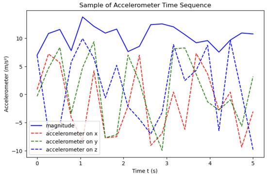
Figure 1.
Accelerometer time sequence: accelerations (dashed red, green, blue), with magnitude (solid).
Table 1 summarizes the gait features engineered from accelerometer data along with their application domains and units. Time-domain features capture temporal gait characteristics (for example, cadence, step time), while statistical measures (for example, skewness, kurtosis) reflect signal distribution. Frequency-domain features (for example, average power, harmonic ratio) characterize rhythmicity, and nonlinear metrics (for example, entropy, regression trends) capture signal complexity. Together, these features captures a holistic profile of gait relevant to alcohol, clinical, and behavioral contexts. We discovered that feature performance may be influenced by the methods used to generate them. Thus, we explored three approaches—Welch power spectral density, fast Fourier transform (FFT), and discrete cosine transform (DCT)—for computing the ratio of spectral peak feature, increasing the total number of features compared to 30.

Table 1.
Accelerometer gait features, their original use cases, and units or variable types.
To account for individual gait differences, all features are normalized by dividing each subject’s feature by its sober walk value. The impact of each type of feature on classification accuracy is evaluated individually and in feature families. The accuracy of random forest, support vector machine (SVM), and naive Bayes classifiers is compared across feature families. Classification results include accuracy, precision, recall, ROC curves, and confusion matrices.
2.1.1. Time-Domain Features
The time-domain features explored in this work are summarized in Table 2.
Table 2.
Time-domain features extracted from accelerometer data.
The time-domain features listed in Table 2 are extracted from accelerometer signals using statistical gait analysis methods. For instance, skewness and kurtosis characterize the distribution shape of the signal values, while step time and cadence capture temporal gait patterns. In these formulas, denotes the ith sample in the time series, is the mean, represents individual step intervals, and is the probability of occurrence of a given feature pattern used for entropy calculation. The harmonic ratio () is computed from the discrete Fourier transform (DFT) components to quantify gait symmetry. These features collectively quantify the variability, regularity, and rhythmicity of walking patterns under different conditions.
2.1.2. Frequency-Domain Features
The frequency-domain features explored in this work are summarized in Table 3. For the ratio of the spectral peak feature, different discrete wavelength transform (DFT) methods were trialed to generate this feature in order to find which of the DFT methods could most improve the performance of frequency-domain features. In this study, the effect of different time–frequency transform methods on a feature were also investigated. In total, 3 alternative methods (default Welch transform, FFT, and DCT) were implemented to calculate this feature. Of the 3 approaches, FFT performed best. Welch, which refers to the Welch’s overlapped segment averaging estimator, is usually a good approach under many conditions. However, due to segmentation in preprocessing and the limit of data length, FFT performed better. The performance of these three approaches are reported in Section 3. For our study, the following features were applied to the gyroscope data only: energy in band 0.5 to 3 Hz, windowed energy in band 0.5 to 3 Hz, regression line for windowed energy.
Table 3.
Frequency-domain features extracted from accelerometer data.
The frequency-domain features listed in Table 3 are derived using spectral analysis techniques such as the Fourier transform, Welch’s method, and DCT. These features capture the periodic and harmonic properties of walking patterns. For instance, average power measures the energy distribution over the frequency spectrum, while the ratio of spectral peaks (RSP) reflects dominant frequency components. SNR and THD quantify the strength and purity of the signal. Energy in specific bands (e.g., 0.5–3 Hz) and windowed band energy reflect the frequency content of gait cycles. The spectral centroid and bandwidth describe how power is spread across frequencies, and regression analysis on windowed energy reveals trends in signal power over time. In the formulas, denotes the spectral representation of the signal, indicates power at frequency f, and corresponds to the spectrum in the ith window.
2.1.3. Wavelet-Domain Features
The wavelet-domain features refer to the features in the time–frequency domain. They are generated from wavelet transform. The features of the wavelet domain explored in this work are summarized in Table 4.
Table 4.
Wavelet-domain features extracted from the signal.
2.1.4. Statistical Features
The statistical features investigated in this study are summarized in Table 5.
Table 5.
Statistical Features.
Although some features such as kurtosis and standard deviation appear in both the time and statistical domains, they are computed from distinct signal representations. Time-domain features are extracted from raw, segmented gait signals, whereas statistical features are derived from transformed or aggregated versions of the signal that capture global patterns across time or frequency.
2.1.5. Information-Theoretic Features
The information-theoretic features investigated in this study are summarized in Table 6.
Table 6.
Information-Theoretic Features.
In total, 27 out of 30 introduced features were investigated for this study.
2.2. Data
The steps described in this section include our procedures for data collection, noise reduction, feature extraction and normalization. This processing flow is illustrated in Figure 2. Our pipeline starts with data collection, then the data is preprocessed, and we perform feature extraction on the preprocessed data in the time, frequency, wavelet, statistical, and information-theoretic domains. Additionally, we added a normalization operation after the feature extraction step. The extracted features are classified using selected models.
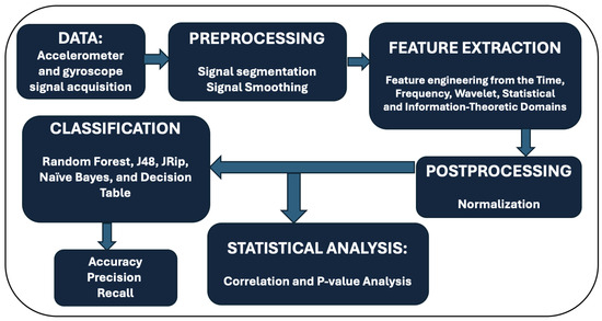
Figure 2.
Work flow of signal process and analysis.
Data Collection and Dataset Summary
Aiello et al. [65] conducted a 5-week study collecting gait data from 24 participants using the MATLAB version 9.0 (R2016a) mobile app to sample accelerometer and gyroscope data from smartphones during walking. Intoxication simulation was achieved by having participants wear special goggles designed to simulate different BAC levels. The resulting data, including timestamps, was saved in CSV files for further analysis. This work focuses on signal processing features extracted from accelerometer data, excluding gyroscope data, with measurements represented in the x, y, and z axes. Nine subjects were excluded due to unreliable or insufficient data. Each subject performed 60 walking trials, with 5 segments corresponding to BAC levels of 0, 0.05, 0.12, 0.2, and 0.3, and with each segment lasting a minimum of 5 s. It is instructive to note that the study was approved by the university’s IRB. All participants gave their informed consent, and no actual alcohol was consumed; intoxication was simulated using certified drunk goggles/busters. A synthetic version of our dataset can be found in Supplementary Materials.
2.3. Data Preprocessing
Our preprocessing steps consist of segmentation at the beginning and a smoothing method to remove noise. Since the data was collected in 5 s segments, there was no need to segment the data. To smooth the data, a moving-average method shown in Equation (2) was used to average out windows of accelerometer signals to reduce noise. The moving-average calculation replaces each value in the sequence with the average of several points around it. We chose to average windows of 5 values, which balances both accuracy and time cost. Figure 3a shows the moving-average smoothened signal vs. non-smoothened signal. Since signal-to-noise ratio (SNR) is one of our features, which relies on the noise, SNR was calculated before the moving average was applied.
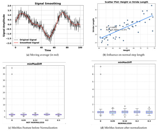
Figure 3.
(a) Moving average smoothing effect. (b) Step length influence on normal step length. (c) MinMax feature scaling before normalization. (d) MinMax feature scaling after normalization.
After calculating features using their definition equations, normalization, shown in Equation (3), was applied to the features to account for variations in the walking styles of various people. For example, people with different height may have different normal step length, as shown in Figure 3b. Normalization will reduce such influences from the feature to give a more accurate result. Figure 3c,d shows the minimum–maximum difference feature before and after normalization.
Correlation-Based Feature Selection
We used CFS to identify the best features for gait classification. CFS selects features highly correlated with BAC levels but uncorrelated with each other. For each feature class, we compute correlations with BAC levels and their p-values. Features with p-values < 0.05 are retained, regardless of correlation strength, for supervised learning. This process is applied to all feature classes. Equation (4) shows the correlation coefficient used for ranking the features based on p-values.
As shown in Table 7, 12 out of 13 time-domain features had a p-value < 0.05 and were useful for alcohol consumption detection. Normalization further increased the correlation of all 12 features by an average of 0.1061. As shown in Table 8, 8 out of 11 features were statistically significant (p-value < 0.05) and were useful for alcohol consumption detection. Seven of these eight frequency-domain features showed stronger correlation after normalization by an average of 0.0999.
Table 7.
Time-domain features ranked by correlation coefficient.
Table 8.
Frequency-domain features ranked by correlation coefficient.
As shown in Table 9, 1 of the 2 wavelet-domain features was useful for the detection of alcohol consumption. Normalization does not improve the performance of the wavelet-domain features. This probably results from the properties of the wavelet domain. The wavelet domain is a time–frequency domain that reflects not only time and frequency properties but also the relationship between time and frequency. However, the normalization process, which usually resizes the range of feature values, can reshape the relationship between time and frequency, causing a decrease in the feature correlation coefficient. Specifically, wavelet features preserve both temporal and spectral structures across multiple scales and inherently encode relative magnitudes. As such, they exhibit a degree of scale invariance, reducing the effect of normalization. As shown in Table 10, all 3 features had a p-value < 0.05 and were useful for alcohol consumption detection. Additionally, all 3 features showed stronger correlation after normalization. Table 11 shows that 1 feature had a p-value < 0.05 and was useful for alcohol consumption detection. Furthermore, this feature showed a stronger correlation with BAC levels after normalization.
Table 9.
Wavelet-domain features ranked by correlation coefficient.
Table 10.
Statistical-Domain features ranked by correlation coefficient.
Table 11.
Information-theoretic features ranked by correlation coefficient.
The features with p-values < 0.05 were classified using the WEKA machine learning library using 10-fold cross-validation at the subject level. Overall average metrics are reported. Since our dataset included data from 15 unique subjects, we partitioned the data into 10 mutually exclusive folds, each containing either 1 or 2 subjects. In each iteration, 9 folds (representing approximately 13–14 subjects) were used for training and validation, while the remaining fold (1–2 subjects) was held out for testing. This ensured that data from any individual subject appeared in only one fold per iteration, preventing data leakage and maintaining subject independence across train–test splits.
2.4. Machine Learning Classifiers
In this work, we compared five popular classifiers: random forest, J48, JRip, naive Bayes, and decision table. These classifiers perform well on small datasets, are robust to overfitting, and have been utilized by prior work on human gait recognition and alcohol intoxication detection [66,67,68,69,70,71]. We applied classification to features with a p-value of < 0.05 Random forest is an ensemble learning method that constructs multiple decision trees for classification, regression, and other tasks. It makes predictions by averaging outputs or selecting the most frequently predicted class, mitigating the tendency of individual decision trees to overfit [72,73]. J48 is a decision tree classifier that generates pruned or unpruned C4.5 decision trees. Developed by Ross Quinlan [74], C4.5 is a classification algorithm that constructs decision trees based on information entropy [75] as shown in Equation (5), in order to maximize the information gain at each step. It is widely regarded as a statistical classifier [76].
JRip, based on the repeated incremental pruning to produce error reduction algorithm by William W. Cohen [77], is an optimized version of incremental reduced error pruning. It splits training data into a growing set and a pruning set, first forming an initial rule set. The rule set is then iteratively pruned using operators that minimize error in the pruning set. The process stops when further pruning increases the error.
Naive Bayes classifiers are probabilistic models based on Bayes’ theorem, shown in Equation (6), with independence assumptions between features. In WEKA, the naive Bayes classifier applies the “maximum a posteriori” (MAP) rule shown in (7) to maximize the prior probability distribution, as shown in Equation (3). This approach makes naive Bayes highly scalable, with parameters scaling linearly with the number of features [75,78].
SVM, based on Vapnik’s statistical learning theory, solves binary classification problems by finding an optimal separating hyperplane (OSH) that maximizes the margin between classes. The points on the margin’s edge, called support vectors, define the OSH. In WEKA, SVM is implemented using the sequential minimal optimization (SMO) algorithm [79,80]. A decision table elegantly maps conditions to corresponding actions, similar to flowcharts and if-then-else statements. Each decision represents a variable or predicate with possible values, while actions define operations to perform based on condition alternatives.
2.5. Evaluation
Evaluation Metrics
A confusion matrix quantifies the performance of a classification model by detailing the distribution of correctly and incorrectly predicted samples across different classes. Table 12 shows a confusion matrix skeleton. The equations for true positive rate, false positive rate, precision, recall, and F1-score are given by Equations (8), (9) and (11)–(13).
Table 12.
Confusion matrix representation.
The ROC area represents the area under the ROC curve, which plots the true positive rate (TPR) against the false positive rate (FPR) across thresholds. It quantifies classifier performance, with a higher area indicating better discrimination. When normalized, it equals the probability that a randomly chosen positive instance ranks higher than a negative one.
3. Results
3.1. Time-Domain Features’ Classification Results
The 12 features of the time domain with p-values < 0.05 were classified using the WEKA machine learning library using 10-fold cross-validation, and the average accuracy across all folds is reported for each of the classifiers. Table 13 shows the results of classifying the time-domain features with p-values < 0.05. The random forest classifier had the best results, with an accuracy of 83.22%.
Table 13.
Classifiers ranked by accuracy for time-domain features with p-values < 0.05.
Other classification performance metrics are reported for different BAC classes in Table 14 for the random forest classifier.
Table 14.
Random forest classifier performance metrics for different BAC Classes.
Figure 4 summarizes the confusion matrix performance of the random forest classifier on time-domain features with p-values < 0.05. The classifier showed high classification ability, with leading values in the diagonal of the confusion matrix.
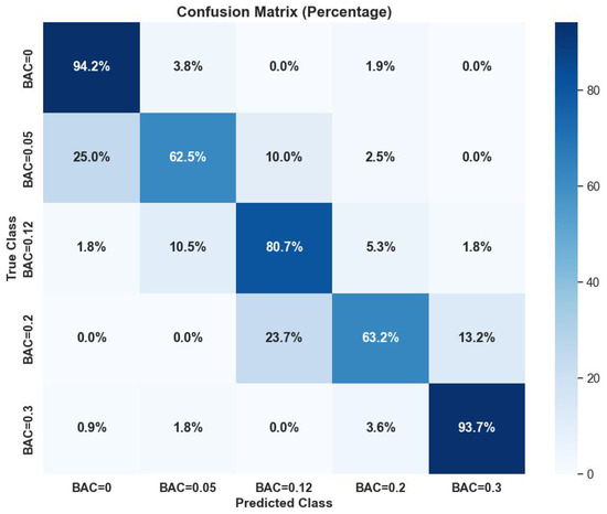
Figure 4.
Random forest classifier confusion matrix performance on time-domain features with p-values < 0.05.
Table 15 shows the WEKA configuration for this best-performing random forest classifier for the time domain.
Table 15.
Random forest configuration for time-domain features.
3.2. Frequency Domain Classification Results
The classification results of the frequency domain features with p-values < 0.05 are reported in Table 16. The J48 classifier had the best results, with an accuracy of 82.21%.
Table 16.
Classifier accuracy comparison on frequency-domain features with p-values < 0.05.
Extensive classification performance metrics are reported for different BAC classes in Table 17 for the best-performing J48 classifier.
Table 17.
J48 classifier performance metrics for different BAC classes.
Figure 5 visualizes the confusion matrix performance of the J48 classifier on frequency-domain features with p-values < 0.05. The classifier showed high classification ability, with leading values in the diagonal of the confusion matrix.
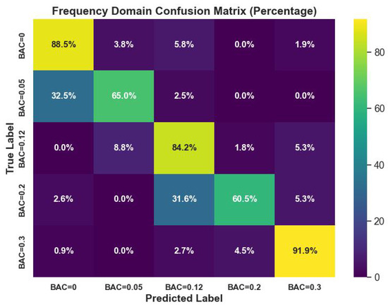
Figure 5.
J48 classifier confusion matrix performance on frequency-domain features with p-values < 0.05.
Table 18 shows the model configuration for this J48 classifier in WEKA.
Table 18.
J48 configuration for frequency-domain features.
3.3. Wavelet-Domain Classification Results
Table 19 shows the accuracy ranking of all classifiers on the wavelet-domain features with p-values < 0.05. The random forest classifier ranked the best, with an accuracy of 77.45%.
Table 19.
Classifiers ranked by accuracy for wavelet-domain features with p-values < 0.05.
Table 20 reports more classification metrics for different BAC classes for the best-performing random forest classifier on wavelet-domain features with p-values < 0.05.
Table 20.
Performance metrics for different BAC classes.
Figure 6 visualizes the confusion matrix performance of the random forest classifier on these wavelet-domain features. The classifier showed high classification ability, with leading values in the diagonal of the confusion matrix.
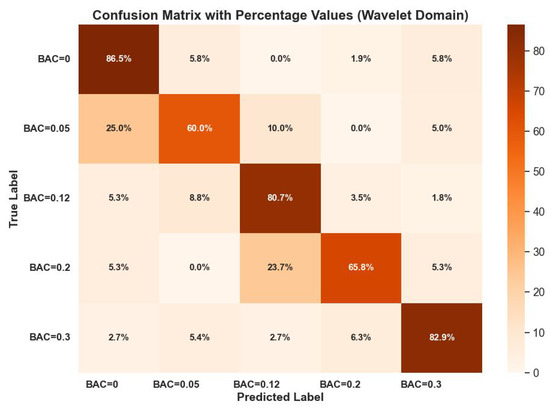
Figure 6.
Random forest classifier confusion matrix performance on wavelet-domain features with p-values < 0.05.
Table 21 shows the model configuration for the best-performing random forest model for the wavelet-domain features.
Table 21.
Random forest configuration for wavelet-domain features.
3.4. Statistical Domain Classification Results
Table 22 shows the classification accuracy ranking of all classifiers for the statistical domain features with p-values < 0.05. The J48 classifier outperformed other classifiers, with 83.89% accuracy.
Table 22.
Classifiers ranked by accuracy for statistical domain features with p-values < 0.05.
Table 23 reports more classification metrics for different BAC classes for the best-performing random forest classifier on statistical domain features with p-values < 0.05.
Table 23.
J48 performance metrics for statistical features with p-values < 0.05.
Figure 7 visualizes the confusion matrix performance of the random forest classifier on these statistical domain features. The classifier showed high classification ability, with leading values in the diagonal of the confusion matrix.
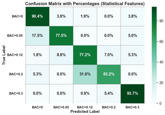
Figure 7.
J48 classifier confusion matrix performance on statistical domain features with p-values < 0.05.
Table 24 summarizes the model random forest model configuration for statistical domain features.
Table 24.
J48 configuration for statistical domain features.
3.5. Information-Theoretic Domain Classification Results
The classification results of the information-theoretic domain features with p-values < 0.05 are reported in Table 25. The random forest classifier reported the best accuracy of 58.05%.
Table 25.
Classifiers ranked by accuracy for information-theoretic features with p-values < 0.05.
Extensive classification performance metrics for different BAC classes are summarized in Table 26 for the random forest classifier.
Table 26.
Performance metrics for different BAC classes.
Figure 8 visualized the confusion matrix performance of the random forest classifier on information-theoretic domain features with p-values < 0.05. The classifier struggled to classify BAC classes 0.12, 0.2 due to low amounts of data in those classes.
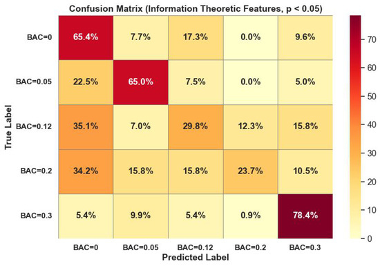
Figure 8.
Random forest classifier confusion matrix performance on information-theoretic domain features with p-values < 0.05.
Table 27 summarizes the model configuration for this random forest classifier for information-theoretic domain features.
Table 27.
Random forest configuration for information-theoretic domain features.
3.6. All Domain Classification Results
Twenty-two (22) features with p-values < 0.05 were used in the supervised classification of gait BAC levels in WEKA with 10-fold cross-validation, yielding an accuracy of 84.90% using the random forest classifier. Table 28 summarizes the classifier results for all features.
Table 28.
Accuracy of different classifiers for all domain features.
Table 29 summarizes the performance metrics for the best-performing classifier (random forest) on features with p-values < 0.05 across all domains.
Table 29.
Performance metrics for different BAC classes.
Figure 9 shows the confusion matrix for the random forest classifier on all domain features with p-values < 0.05. The leading values on the diagonal show the classification accuracy of the classifier in accurately classifying data samples in their respective classes.
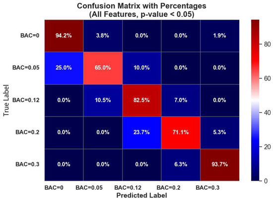
Figure 9.
Random forest classifier confusion matrix performance on all domain features with p-values < 0.05.
Table 30 shows the model configuration random forest for all-domain feature classification.
Table 30.
Random forest configuration for all domain features.
3.7. Comparison to Prior Work
We compared our study with prior similar works, and we summarize our findings in Table 31. Prior works were similar in several ways but differed in other ways from our work, limiting a fair comparison. Both Bremner et al. and McAfee et al. utilized data in which intoxication was simulated using drunk buster goggles, but they combined data collected from both a smartphone and a smartwatch. As we collect data only from a smartphone, we compare our results to the results they achieved on only their smartphone dataset. Our results from classifying all domain features outperformed prior work by Bremner et al. [81] with a 22.9% increase in accuracy. There were other notable differences. Bremner et al. utilized a deep learning model, while our work utilized traditional machine learning on handcrafted features. Additionally, while our dataset was balanced, Bremner et al. utilized a highly imbalanced dataset, but did not report their AUC or F1-score, a more useful metric for imbalanced datasets. Our study, on the other hand, did not overfit to our small dataset and reported an impressive AUC score of 0.928. While McAfee et al. achieved 89.45% accuracy using skew, kurtosis, gait velocity, residual step time, band power, XZ sway, XY sway, YZ sway, and sway volume features, primarily from gait and postural sway domains, our work explored a broader set of 27 features spanning time, frequency, statistical, wavelet, and information-theoretic domains, as shown in Table 1. Despite using a smaller dataset, our model achieved 84.90% accuracy, demonstrating that our more diverse feature set captures complex patterns that should generalize well to real-world variability. Also, with the expanded number of features across different domains and the utilization of 10-fold cross-validation, our work achieves a stronger subject-level generalization compared to previous works that utilize fewer predictive features.
Table 31.
Comparison of performance metrics with prior work.
4. Discussion
Based on the results presented in the previous section, several key findings are presented.
First, the analysis of the boxplot and predictability report indicates that normalization significantly enhances the performance of most features. Specifically, 20 out of 22 features with p-values < 0.05 showed improvement after normalization. This finding supports existing research that emphasizes the role of data normalization or standardization in improving machine learning performance on sensor data [83]. Particularly, preprocessing was found to significantly boost the performance of random forest classifiers on human activity recognition gait data, a finding consistent with our results.
Second, statistical-domain features exhibited the highest predictive accuracy of 83.89%. This was followed by time-domain features with an accuracy of 83.22%, and frequency-domain features, which achieved an accuracy of 82.21%. These results highlight the importance of statistical properties in distinguishing patterns within the data. Above all, our findings align with previous findings that statistical features such as kurtosis provide rich descriptors of motion patterns [84]. This work aligns with our findings that time and frequency domain features are top performers as well, after statistical features. It is worthy of note that some features can be categorized as both statistical and time-domain features. Our results strengthen the argument for prioritizing statistical features in intoxication detection.
Third, the frequency-domain features may benefit from the application of time–frequency transform techniques. Preliminary experiments suggest that p-values vary depending on the choice of spectral estimation method, such as Welch, FFT, and DCT, when computing the ratio of spectral peaks. This highlights the potential for further optimization using advanced spectral analysis techniques.
Fourth, most extracted features demonstrate strong predictive capabilities. Out of the 27 tested features, 22 features have shown strong predictive capabilities. The results suggest that refining and optimizing feature extraction methods could further enhance classification accuracy.
Limitations and Areas for Improvement
First, our study had a limited dataset with 15 unique subjects whose data were pre-processed and classified by our traditional machine learning models. Most models would struggle or overfit if trained on very small dataset like ours. Our results can be improved with large amounts of data, which will enable models to learn gait patterns associated with alcohol consumption and intoxication. Viable next steps include implementing data augmentation strategies and exploring deep learning approaches such as few-shot and meta-learning, which are suited to small datasets.
Second, exploration of more classifiers will improve our work. Even though our study achieved good results with the five selected classifiers, we can improve our study performance by testing a wider range of classifiers, including ensemble techniques.
Third, working with a real alcohol dataset is necessary to validate our work. Real alcohol intoxication causes widespread physiological and psychological changes, impairing cognition (judgment, decision-making, reaction time) and physical functions (coordination, balance, vision) [85]. In contrast, “Drunk Busters” goggles simulate only visual impairments—such as distortion of depth perception and reduced peripheral vision—without replicating alcohol’s broader cognitive and physiological changes [85]. Hence, drunk buster goggles may not capture all the effects and variabilities real alcoholic drinks will have on a subject [86]. These factors limit the validity and generalizability of our findings. However, the use of goggles provides a safe and controlled proxy for early investigation and model evaluation. Future work will focus on collecting real intoxication data to validate our findings.
Fourth, statistical significance testing is needed to validate our model’s performance. While our current study provided a comparative analysis of different classifier performances using established metrics, statistical significance testing using methods like ANOVA or the Wilcoxon signed-rank test was not performed. Our future research would include these tests to strengthen comparative claims and support performance differences with statistical rigor.
5. Conclusions
This study proposes a machine learning approach to detect alcohol intoxication using small gait data gathered from smartphone sensors. Specifically, this work comprehensively compares smartphone accelerometer gait features extracted from the time, frequency, wavelet, information-theoretic and statistical domains. Our data preprocessing pipeline included computing moving averages to smooth out spurious signals and remove noise, feature normalization, and feature selection using a correlation-based coefficient approach. Our study showed that 22 out of the 27 features had strong predictive capabilities with p-values < 0.05. Furthermore, results showed that statistical features had the highest predictive accuracy, with 83.89%, followed by time-domain features, with an accuracy of 83.22%, and frequency-domain features, which attained an accuracy of 82.21%. As part of our future research direction, we plan to rigorously evaluate the statistical significance and utility of additional features including the Lempel–Ziv complexity, regression line for local maxima and minima (which requires walked distance to be calculated), and regression lines for windowed energy (which require walked distance to be calculated). Additionally, we plan to collect additional data that would enable us to explore deep learning approaches, which have demonstrably outperformed traditional machine learning models if adequate data is available.
Supplementary Materials
The following supporting information can be downloaded at: https://www.mdpi.com/article/10.3390/app15137250/s1.
Author Contributions
Conceptualization, methodology, formal analysis, software, validation, and writing—original draft preparation, M.Q.; writing—review and editing, literature review, synthetic data generation, and data and results visualization, S.C.U.; supervision, resources, project administration, and funding acquisition, E.A. All authors have read and agreed to the published version of the manuscript.
Funding
This research received no external funding.
Institutional Review Board Statement
Not applicable.
Informed Consent Statement
Not applicable.
Data Availability Statement
Data is unavailable due to privacy concerns. However, a synthetic dataset, replicating the statistical properties of the original data, will be made available for reproducibility and benchmarking purposes.
Acknowledgments
The authors would like to thank Worcester Polytechnic Institute for their institutional support.
Conflicts of Interest
Author Muxi Qi was employed by Diamond Diagnostics Inc. The remaining authors declare that the research was conducted in the absence of any commercial or financial relationships that could be construed as a potential conflict of interest.
References
- Gallup. More Than Six in 10 Americans Drink Alcohol. Available online: https://news.gallup.com/poll/509501/six-americans-drink-alcohol.aspx (accessed on 24 March 2025).
- Substance Abuse and Mental Health Services Administration (SAMHSA), Center for Behavioral Health Statistics and Quality. 2023 National Survey on Drug Use and Health. Table 2.27A—Alcohol Use in Past Month: Among People Aged 12 or Older; By Age Group and Demographic Characteristics, Numbers in Thousands, 2022 and 2023. Available online: https://www.samhsa.gov/data/report/2023-nsduh-detailed-tables (accessed on 23 February 2025).
- Substance Abuse and Mental Health Services Administration (SAMHSA), Center for Behavioral Health Statistics and Quality. 2023 National Survey on Drug Use and Health. Table 2.27B—Alcohol Use in Past Month: Among People Aged 12 or Older; By Age Group and Demographic Characteristics, Percentages, 2022 and 2023. Available online: https://www.samhsa.gov/data/report/2023-nsduh-detailed-tables (accessed on 23 February 2025).
- Substance Abuse and Mental Health Services Administration (SAMHSA), Center for Behavioral Health Statistics and Quality. 2023 National Survey on Drug Use and Health. Table 2.28A—Binge Alcohol Use in Past Month: Among People Aged 12 or Older; By Age Group and Demographic Characteristics, Numbers in Thousands, 2022 and 2023. Available online: https://www.samhsa.gov/data/report/2023-nsduh-detailed-tables (accessed on 23 February 2025).
- Substance Abuse and Mental Health Services Administration (SAMHSA), Center for Behavioral Health Statistics and Quality. 2023 National Survey on Drug Use and Health. Table 2.28B—Binge Alcohol Use in Past Month: Among People Aged 12 or Older; By Age Group and Demographic Characteristics, Percentages, 2022 and 2023. Available online: https://www.samhsa.gov/data/report/2023-nsduh-detailed-tables (accessed on 23 February 2025).
- Substance Abuse and Mental Health Services Administration (SAMHSA), Center for Behavioral Health Statistics and Quality. 2023 National Survey on Drug Use and Health. Table 2.29A—Heavy Alcohol Use in Past Month: Among People Aged 12 or Older; by Age Group and Demographic Characteristics, Numbers in Thousands, 2022 and 2023. Available online: https://www.samhsa.gov/data/report/2023-nsduh-detailed-tables (accessed on 25 February 2025).
- Substance Abuse and Mental Health Services Administration (SAMHSA), Center for Behavioral Health Statistics and Quality. 2023 National Survey on Drug Use and Health. Table 2.29B—Heavy Alcohol Use in Past Month: Among People Aged 12 or Older; By Age Group and Demographic Characteristics, Percentages, 2022 and 2023. Available online: https://www.samhsa.gov/data/report/2023-nsduh-detailed-tables (accessed on 25 February 2025).
- Wilcockson, T.D.W.; Roy, S. Could Alcohol-Related Cognitive Decline Be the Result of Iron-Induced Neuroinflammation? Brain Sci. 2024, 14, 520. [Google Scholar] [CrossRef] [PubMed]
- Vore, A.S.; Deak, T. Alcohol, Inflammation, and Blood-Brain Barrier Function in Health and Disease Across Development. Int. Rev. Neurobiol. 2022, 161, 209–249. [Google Scholar] [CrossRef] [PubMed]
- National Cancer Institute. Alcohol Consumption. Cancer Trends Progress Report. 2024. Available online: https://progressreport.cancer.gov/prevention/diet_alcohol/alcohol (accessed on 20 May 2025).
- Rutgers Cancer Institute of New Jersey. Liver Cancer, Excessive Alcohol Use, and Other Risks. 2024. Available online: https://cinj.org/liver-cancer-excessive-alcohol-use-and-other-risks (accessed on 20 May 2025).
- World Health Organization. No Level of Alcohol Consumption Is Safe for Our Health. 2023. Available online: https://www.who.int/europe/news/item/04-01-2023-no-level-of-alcohol-consumption-is-safe-for-our-health (accessed on 20 May 2025).
- U.S. Department of Health and Human Services. Alcohol and Cancer Risk. Office of Disease Prevention and Health Promotion. 2023. Available online: https://www.hhs.gov/sites/default/files/oash-alcohol-cancer-risk.pdf (accessed on 20 May 2025).
- Bagnardi, V.; Rota, M.; Botteri, E.; Tramacere, I.; Islami, F.; Fedirko, V.; Scotti, L.; Jenab, M.; Turati, F.; Pasquali, E.; et al. Alcohol consumption and site-specific cancer risk: A comprehensive dose–response meta-analysis. Br. J. Cancer 2015, 112, 580–593. [Google Scholar] [CrossRef] [PubMed]
- Centers for Disease Control and Prevention. Estimated Liver Disease Deaths Include Deaths with Underlying Causes Coded as Alcoholic Liver Disease (K70); Liver Cirrhosis, Unspecified (K74.0–K74.2, K74.6, K76.0, K76.7, and K76.9); Chronic Hepatitis (K73); Portal Hypertension (K76.6); Liver Cancer (C22); or Other Liver Diseases (K71, K72, K74.3–K74.5, K75, K76.1–K76.5, and K76.8). Available online: https://ftp.cdc.gov/pub/Health_Statistics/NCHS/Datasets/DVS/mortality/mort2023us.zip (accessed on 19 February 2025).
- Number of Deaths from Multiple Cause of Death Public-Use Data File. 2023; lcohol-Attributable Fractions (AAFs) from CDC 51 Alcohol-Related Disease Impact; Prevalence of Alcohol Consumption from the National Survey on Drug Use and Health, 2023, 52 for Estimating Indirect AAFs for Chronic Hepatitis and Liver Cancer. Available online: https://nccd.cdc.gov/DPH_ARDI/Default/Default.aspx (accessed on 19 February 2025).
- Centers for Disease Control and Prevention. Alcohol Use and Health. Available online: http://www.cdc.gov/alcohol/fact-sheets/alcohol-use.htm (accessed on 19 February 2025).
- Legends Recovery. Economic Effects of Alcohol and Drugs. Available online: https://www.legendsrecovery.com/blog/economic-effects-of-alcohol-and-drugs (accessed on 6 February 2025).
- Intoxalock. BAC vs. BrAC: What’s the Difference? Available online: https://www.intoxalock.com/knowledge-center/bac-vs-brac-whats-the-difference (accessed on 19 May 2025).
- Walden, K.-R.; Saldich, E.B.; Wong, G.; Liu, H.; Wang, C.; Rosen, I.G.; Luczak, S.E. Chapter Seven—Momentary Assessment of Drinking: Past Methods, Current Approaches Incorporating Biosensors, and Future Directions. In Psychology of Learning and Motivation; Federmeier, K.D., Ed.; Academic Press: Cambridge, MA, USA, 2023; Volume 79, pp. 271–301. ISBN 9780443193866. [Google Scholar] [CrossRef]
- Wang, Y.; Fridberg, D.J.; Leeman, R.F.; Cook, R.L.; Porges, E.C. Wrist-Worn Alcohol Biosensors: Strengths, Limitations, and Future Directions. Alcohol 2019, 81, 83–92. [Google Scholar] [CrossRef]
- American Addiction Centers. Alcohol Moderation Management: Programs and Steps to Control Drinking. Available online: https://americanaddictioncenters.org/blog/alcohol-moderation-management (accessed on 19 May 2025).
- Dasgupta, P.; VanSwearingen, J.; Godfrey, A.; Redfern, M.; Montero-Odasso, M.; Sejdic, E. Acceleration Gait Measures as Proxies for Motor Skill of Walking: A Narrative Review. IEEE Trans. Neural Syst. Rehabil. Eng. 2021, 29, 249–261. [Google Scholar] [CrossRef]
- Gundersen Health. Under the Influence: The Effects of Alcohol on the Body. Gundersen Health System. 2023. Available online: https://www.gundersenhealth.org/health-wellness/staying-healthy/under-the-influence-the-effects-of-alcohol-on-the-body (accessed on 25 May 2025).
- Vassar, R.L.; Rose, J. Motor Systems and Postural Instability. In Handbook of Clinical Neurology; Sullivan, E.V., Pfefferbaum, A., Eds.; Elsevier: Amsterdam, The Netherlands, 2014; Volume 125, pp. 237–251. ISBN 9780444626196. ISSN 0072-9752. [Google Scholar] [CrossRef]
- Mistarz, N.; Canfield, L.; Nielsen, D.G.; Skøt, L.; Mellentin, A.I. Gait Ataxia in Alcohol Use Disorder: A Systematic Review. Psychol. Addict. Behav. 2024, 38, 507–517. [Google Scholar] [CrossRef]
- Oscar-Berman, M.; Valmas, M.M.; Sawyer, K.S.; Mosher Ruiz, S.; Luhar, R.B.; Gravitz, Z.R. Profiles of Impaired, Spared, and Recovered Neuropsychologic Processes in Alcoholism. In Handbook of Clinical Neurology; Sullivan, E.V., Pfefferbaum, A., Eds.; Elsevier: Amsterdam, The Netherlands, 2014; Volume 125, pp. 183–210. ISBN 9780444626196. ISSN 0072-9752. [Google Scholar] [CrossRef]
- Demura, S.; Uchiyama, M. Influence of Moderate Alcohol Ingestion on Gait. Sport Sci. Health 2008, 4, 21–26. [Google Scholar] [CrossRef]
- Calhoun, V.D.; Carvalho, K.; Astur, R.; Pearlson, G.D. Using Virtual Reality to Study Alcohol Intoxication Effects on the Neural Correlates of Simulated Driving. Appl. Psychophysiol. Biofeedback 2005, 30, 285–306. [Google Scholar] [CrossRef]
- Promises Behavioral Health. Alcoholism and Ataxia: What’s the Connection? Available online: https://www.promises.com/addiction-blog/alcoholism-and-ataxia/ (accessed on 25 May 2025).
- Gimunová, M.; Bozděch, M.; Novák, J.; Svoboda, Z.; Zvoníček, J.; Bizovská, L.; Janura, M. Gender Differences in the Effect of a 0.11% Breath Alcohol Concentration on Forward and Backward Gait. Sci. Rep. 2022, 12, 18773. [Google Scholar] [CrossRef]
- Mount Sinai Health Library. Alcoholic Neuropathy. Mount Sinai Health Library. 2023. Available online: https://www.mountsinai.org/health-library/diseases-conditions/alcoholic-neuropathy (accessed on 25 February 2025).
- Meigal, A.Y.; Gerasimova-Meigal, L.I.; Reginya, S.A.; Soloviev, A.V.; Moschevikin, A.P. Gait Characteristics Analyzed with Smartphone IMU Sensors in Subjects with Parkinsonism under the Conditions of “Dry” Immersion. Sensors 2022, 22, 7915. [Google Scholar] [CrossRef]
- Baek, J.-E.; Jung, J.-H.; Kim, H.-K.; Cho, H.-Y. Smartphone Accelerometer for Gait Assessment: Validity and Reliability in Healthy Adults. Appl. Sci. 2024, 14, 11321. [Google Scholar] [CrossRef]
- ConsumerAffairs. Cell Phone Statistics 2024. ConsumerAffairs.com. Available online: https://www.consumeraffairs.com/cell_phones/cell-phone-statistics.html (accessed on 19 February 2025).
- Henriksen, M.; Lund, H.; Moe-Nilssen, R.; Bliddal, H.; Danneskiod-Samsøe, B. Test–Retest Reliability of Trunk Accelerometric Gait Analysis. Gait Posture 2004, 19, 288–297. [Google Scholar] [CrossRef] [PubMed]
- Silsupadol, P.; Teja, K.; Lugade, V. Reliability and Validity of a Smartphone-Based Assessment of Gait Parameters across Walking Speed and Smartphone Locations: Body, Bag, Belt, Hand, and Pocket. Gait Posture 2017, 58, 516–522. [Google Scholar] [CrossRef]
- Tao, S.; Zhang, H.; Kong, L.; Sun, Y.; Zhao, J. Validation of Gait Analysis Using Smartphones: Reliability and Validity. Digit. Health 2024, 10, 1–10. [Google Scholar] [CrossRef]
- Arnold, Z.; Larose, D.; Agu, E. Smartphone Inference of Alcohol Consumption Levels from Gait. In Proceedings of the 2015 International Conference on Healthcare Informatics (ICHI), Dallas, TX, USA, 21–23 October 2015; pp. 417–426. [Google Scholar] [CrossRef]
- SCRAM Systems. SCRAM Continuous Alcohol Monitoring. Available online: http://www.scramsystems.com/index/scram/continuous-alcoholmonitoring (accessed on 22 February 2025).
- Tokyoflash Japan. Kisai Intoxicated LCD Watch. Available online: http://www.tokyoflash.com/en/watches/kisai/intoxicated/ (accessed on 22 February 2025).
- Myrecek. AlcoDroid Alcohol Tracker. Available online: https://play.google.com/store/apps/details?id=org.M.alcodroid&hl=en (accessed on 22 February 2025).
- Wichmann, R. IntelliDrink PRO—Blood Alcohol Content (BAC) Calculator. Available online: https://itunes.apple.com/us/app/intellidrink-pro-blood-alcohol/id440759306?mt=8 (accessed on 22 February 2025).
- Cicirelli, G.; Impedovo, D.; Dentamaro, V.; Marani, R.; Pirlo, G.; D’Orazio, T.R. Human Gait Analysis in Neurodegenerative Diseases: A Review. IEEE J. Biomed. Health Inform. 2022, 26, 229–242. [Google Scholar] [CrossRef]
- Kiranyaz, S.; Avci, O.; Abdeljaber, O.; Ince, T.; Gabbouj, M.; Inman, D.J. 1D Convolutional Neural Networks and Applications: A Survey. Mech. Syst. Signal Process. 2021, 151, 107398. [Google Scholar] [CrossRef]
- Ravi, S.; Radhakrishnan, A. A Hybrid 1D CNN-BiLSTM Model for Epileptic Seizure Detection Using Multichannel EEG Feature Fusion. Biomed. Phys. Eng. Express 2024, 10, 035005. [Google Scholar] [CrossRef]
- Pouromran, F.; Lin, Y.; Kamarthi, S. Personalized Deep Bi-LSTM RNN-Based Model for Pain Intensity Classification Using EDA Signal. Sensors 2022, 22, 8087. [Google Scholar] [CrossRef]
- Wallén, M.B.; Nero, H.; Franzén, E.; Hagströmer, M. Comparison of Two Accelerometer Filter Settings in Individuals with Parkinson’s Disease. Physiol. Meas. 2014, 35, 2287. [Google Scholar] [CrossRef]
- Salarian, A.; Russmann, H.; Vingerhoets, F.J.; Dehollain, C.; Blanc, Y.; Burkhard, P.R.; Aminian, K. Gait Assessment in Parkinson’s Disease: Toward an Ambulatory System for Long-Term Monitoring. IEEE Trans. Biomed. Eng. 2004, 51, 1434–1443. [Google Scholar] [CrossRef]
- Kao, H.-L.C.; Ho, B.-J.; Lin, A.C.; Chu, H.-H. Phone-Based Gait Analysis to Detect Alcohol Usage. In Proceedings of the 2012 ACM Conference on Ubiquitous Computing (UbiComp ’12), Pittsburgh, PA, USA, 5–8 September 2012; Association for Computing Machinery: New York, NY, USA, 2012; pp. 661–662. [Google Scholar] [CrossRef]
- Madeleine, P.; Tuker, K.; Arendt-Nielsen, L.; Farina, D. Heterogeneous Mechanomyographic Absolute Activation of Paraspinal Muscles Assessed by a Two-Dimensional Array during Short and Sustained Contractions. J. Biomech. 2007, 40, 2663–2671. [Google Scholar] [CrossRef] [PubMed]
- Montgomery, E.B.U.S., Jr. Neuron signal analysis system and method. U.S. Patent 7,136,696, 2006. [Google Scholar]
- Sejdić, E.; Lowry, K.A.; Bellanca, J.; Redfern, M.S.; Brach, J.S. A Comprehensive Assessment of Gait Accelerometry Signals in Time, Frequency and Time-Frequency Domains. IEEE Trans. Neural Syst. Rehabil. Eng. 2014, 22, 603–612. [Google Scholar] [CrossRef] [PubMed]
- Klucken, J.; Barth, J.; Kugler, P.; Schlachetzki, J.; Henze, T.; Marxreiter, F.; Kohl, Z.; Steidl, R.; Hornegger, J.; Eskofier, B.; et al. Unbiased and Mobile Gait Analysis Detects Motor Impairment in Parkinson’s Disease. PLoS ONE 2013, 8, e56956. [Google Scholar] [CrossRef]
- Porta, A.; Baselli, G.; Liberati, D.; Montano, N.; Cogliati, C.; Gnecchi-Ruscone, T.; Malliani, A.; Cerutti, S. Measuring Regularity by Means of a Corrected Conditional Entropy in Sympathetic Outflow. Biol. Cybern. 1998, 78, 71–78. [Google Scholar] [CrossRef]
- Porta, A.; Guzzetti, S.; Montano, N.; Furlan, R.; Pagani, M.; Malliani, A.; Cerutti, S. Entropy, Entropy Rate, and Pattern Classification as Tools to Typify Complexity in Short Heart Period Variability Series. IEEE Trans. Biomed. Eng. 2001, 48, 1282–1291. [Google Scholar] [CrossRef]
- Akay, M. Noninvasive Diagnosis of Coronary Artery Disease Using a Neural Network Algorithm. Biol. Cybern. 1992, 67, 361–367. [Google Scholar] [CrossRef]
- Lee, J.; Sejdić, E.; Steele, C.M.; Chau, T. Effects of Liquid Stimuli on Dual-Axis Swallowing Accelerometry Signals in a Healthy Population. Biomed. Eng. Online 2010, 9, 7. [Google Scholar] [CrossRef]
- Rosso, O.A.; Blanco, S.; Yordanova, J.; Kolev, V.; Figliola, A.; Schürmann, M.; Başar, E. Wavelet Entropy: A New Tool for Analysis of Short Duration Brain Electrical Signals. J. Neurosci. Methods 2001, 105, 65–75. [Google Scholar] [CrossRef]
- Ferenets, R.; Lipping, T.; Anier, A.; Jäntti, V.; Melto, S.; Hovilehto, S. Comparison of Entropy and Complexity Measures for the Assessment of Depth of Sedation. IEEE Trans. Biomed. Eng. 2006, 53, 1067–1077. [Google Scholar] [CrossRef]
- Lu, H.; Huang, J.; Saha, T.; Nachman, L. Unobtrusive Gait Verification for Mobile Phones. In Proceedings of the 2014 ACM International Symposium on Wearable Computers (ISWC’14), Seattle, WA, USA, 13–17 September 2014; Association for Computing Machinery: New York, NY, USA, 2014; pp. 91–98. [Google Scholar] [CrossRef]
- Brach, J.S.; McGurl, D.; Wert, D.; Vanswearingen, J.M.; Perera, S.; Cham, R.; Studenski, S. Validation of a Measure of Smoothness of Walking. J. Gerontol. A Biol. Sci. Med. Sci. 2011, 66, 136–141. [Google Scholar] [CrossRef]
- Aboy, M.; Hornero, R.; Abásolo, D.; Álvarez, D. Interpretation of the Lempel-Ziv Complexity Measure in the Context of Biomedical Signal Analysis. IEEE Trans. Biomed. Eng. 2006, 53, 2282–2288. [Google Scholar] [CrossRef]
- Lempel, A.; Ziv, J. On the Complexity of Finite Sequences. IEEE Trans. Inf. Theory 1976, 22, 75–81. [Google Scholar] [CrossRef]
- Aiello, C.; Agu, E. Investigating postural sway features, normalization and personalization in detecting blood alcohol levels of smartphone users. In Proceedings of the 2016 IEEE Wireless Health (WH), Bethesda, MD, USA, 25–27 October 2016; pp. 1–8. [Google Scholar] [CrossRef]
- Zhu, X.; Du, X.; Kerich, M.; Lohoff, F.W.; Momenan, R. Random Forest Based Classification of Alcohol Dependence Patients and Healthy Controls Using Resting State MRI. Neurosci. Lett. 2018, 676, 27–33. [Google Scholar] [CrossRef]
- Li, Z.; Wang, H.; Zhang, Y.; Zhao, X. Random Forest–Based Feature Selection and Detection Method for Drunk Driving Recognition. Int. J. Distrib. Sens. Netw. 2020, 16, 1–10. [Google Scholar] [CrossRef]
- Rana, J.; Arora, N.; Hiran, D. Gait Recognition Using J48-Based Identification with Knee Joint Movements. In Proceedings of the International Conference on Soft Computing and Signal Processing (ICSCSP 2018), Hyderabad, India, 22–23 June 2018; Wang, J., Reddy, G., Prasad, V., Reddy, V., Eds.; Advances in Intelligent Systems and Computing; Springer: Singapore, 2019; Volume 900, pp. 169–177. [Google Scholar] [CrossRef]
- Herrera-Alcántara, O.; Barrera-Animas, A.Y.; González-Mendoza, M.; Castro-Espinoza, F. Monitoring Student Activities with Smartwatches: On the Academic Performance Enhancement. Sensors 2019, 19, 1605. [Google Scholar] [CrossRef]
- Shen, J.; Fang, H. Human Activity Recognition Using Gaussian Naïve Bayes Algorithm in Smart Home. J. Phys. Conf. Ser. 2020, 1631, 012059. [Google Scholar] [CrossRef]
- Nurwulan, N.R.; Jiang, B.C. Window Selection Impact in Human Activity Recognition. Int. J. Innov. Technol. Interdiscip. Sci. 2020, 3, 381–394. [Google Scholar]
- Ho, T.K. Random Decision Forests. In Proceedings of the 3rd International Conference on Document Analysis and Recognition (ICDAR), Montreal, QC, Canada, 14–16 August 1995; Volume 1, pp. 278–282. [Google Scholar] [CrossRef]
- Friedman, J.; Hastie, T.; Tibshirani, R. The Elements of Statistical Learning, 2nd ed.; Springer: Berlin/Heidelberg, Germany, 2008. [Google Scholar]
- Salzberg, S.L. C4.5: Programs for Machine Learning by J. Ross Quinlan. Morgan Kaufmann Publishers, Inc., 1993. Mach. Learn. 1994, 16, 235–240. [Google Scholar] [CrossRef]
- Russell, S.; Norvig, P. Artificial Intelligence: A Modern Approach, 2nd ed.; Prentice-Hall: Englewood Cliffs, NJ, USA, 2003. [Google Scholar]
- Umd.edu. Top 10 Algorithms in Data Mining. Available online: http://www.cs.umd.edu/~samir/498/10Algorithms-08.pdf (accessed on 4 March 2025).
- Cohen, W.W. Fast Effective Rule Induction. In Machine Learning Proceedings 1995; Prieditis, A., Russell, S., Eds.; Morgan Kaufmann: San Francisco, CA, USA, 1995; pp. 115–123. ISBN 9781558603776. [Google Scholar] [CrossRef]
- Singh, A. Maximum A Posteriori (MAP) Estimation. Lecture Notes for 10-315: Introduction to Machine Learning, Carnegie Mellon University. 2022. Available online: https://www.cs.cmu.edu/~aarti/Class/10315_Spring22/lecs/MAP.pdf (accessed on 25 May 2025).
- Vapnik, V. The Nature of Statistical Learning Theory; Springer: New York, NY, USA, 2000. [Google Scholar] [CrossRef]
- Begg, R.K.; Palaniswami, M.; Owen, B. Support Vector Machines for Automated Gait Classification. IEEE Trans. Biomed. Eng. 2005, 52, 828–838. [Google Scholar] [CrossRef] [PubMed]
- Bremner, J.; Cheung, N.; Ho Lam, Q.; Huang, S. IntoxiGait: Investigating Deep Learning to Predict Intoxication Levels Using Smartphones and Smartwatches. Major Qualifying Project, Computer Science; Worcester Polytechnic Institute: Worcester, MA, USA, 2025; Available online: https://digital.wpi.edu/concern/parent/1544bq57j/file_sets/1v53jz50f (accessed on 15 June 2025).
- McAfee, A.; Watson, J.; Bianchi, B.; Aiello, C.; Agu, E. AlcoWear: Detecting Blood Alcohol Levels from Wearables. In Proceedings of the 2017 IEEE SmartWorld, Ubiquitous Intelligence & Computing, Advanced & Trusted Computing, Scalable Computing & Communications, Cloud & Big Data Computing, Internet of People and Smart City Innovation (SmartWorld/SCALCOM/UIC/ATC/CBDCom/IOP/SCI), San Francisco, CA, USA, 4–8 August 2017; pp. 1–8. [Google Scholar] [CrossRef]
- Atalaa, B.; Ziedan, I.; Alenany, A.; Helmi, A. Feature Engineering for Human Activity Recognition. Int. J. Adv. Comput. Sci. Appl. 2021, 12, 221. [Google Scholar] [CrossRef]
- Alruban, A.; Alobaidi, H.; Li, N.C.F. Physical Activity Recognition by Utilising Smartphone Sensor Signals. Appl. Sci. 2022, 12, 2201. [Google Scholar] [CrossRef]
- Irwin, C.; Desbrow, B.; McCartney, D. Effects of Alcohol Intoxication Goggles (Fatal Vision Goggles) with a Concurrent Cognitive Task on Simulated Driving Performance. Traffic Inj. Prev. 2019, 20, 777–782. [Google Scholar] [CrossRef] [PubMed]
- Drivers Ed Guru. How Alcohol Impacts Your Ability to Drive. Available online: https://drunkbusters.com/content/drivers-ed-guru.pdf (accessed on 25 May 2025).
Disclaimer/Publisher’s Note: The statements, opinions and data contained in all publications are solely those of the individual author(s) and contributor(s) and not of MDPI and/or the editor(s). MDPI and/or the editor(s) disclaim responsibility for any injury to people or property resulting from any ideas, methods, instructions or products referred to in the content. |
© 2025 by the authors. Licensee MDPI, Basel, Switzerland. This article is an open access article distributed under the terms and conditions of the Creative Commons Attribution (CC BY) license (https://creativecommons.org/licenses/by/4.0/).