Abstract
Transformers have been extensively utilized as encoders in medical image segmentation; however, the information that an encoder can capture is inherently limited. In this study, we propose MINTFormer, which introduces a Heterogeneous encoder that integratesCSWin and MaxViT to fully exploit the potential of encoders with different encoding methodologies. Additionally, we observed that the encoder output contains substantial redundant information. To address this, we designed a Demodulate Bridge (DB) to filter out redundant information from feature maps. Furthermore, we developed a multi-Scale Sampling Decoder (SSD) capable of preserving information about organs of varying sizes during upsampling and accurately restoring their shapes. This study demonstrates the superior performance of MINTFormer across several datasets, including Synapse, ACDC, Kvasir-SEG, and skin lesion segmentation datasets.
1. Introduction
Medical image segmentation models are designed to process pathological images and delineate the shape and structure of lesion areas within the images. These models facilitate the rapid localization of lesions, thereby providing invaluable assistance in medical treatment [1,2,3]. U-Net [4] comprises three primary modules: the encoder, decoder, and skip connections. The encoder–decoder structure of U-Net represents a significant advantage. The encoder progressively reduces the image resolution to extract high-level semantic features, while the decoder progressively increases the resolution to restore these high-level semantic features to a segmentation result that approximates the original image size. This symmetrical structure enables the model to comprehend images at different scales, capturing overall semantic information and recovering detailed information. Skip connections facilitate the transfer of feature information from the encoder to the decoder, preserving local image details. This allows the decoder to utilize the richer, detailed features present in the encoder’s early layers, thereby enhancing segmentation accuracy. The efficacy of the U-Net architecture in medical image segmentation is attributed to these advantages.
Traditional U-Net architecture utilizes a convolutional neural network [5] (CNN) as an encoder to filter irrelevant information and downsample the feature map, preparing it for the subsequent stages where deep semantic information is extracted. Despite its success in medical image segmentation, reliance on CNNs limits the receptive field to a fixed convolution kernel size, hindering U-Net’s ability to capture long-range pixel relationships within the feature map [6,7,8]. To address this limitation, Dai et al. introduced Deformable Convolution and region of interest (RoI) pooling [9], which enhance spatial sampling locations with additional offsets, thereby improving the CNN’s transformation modeling capabilities. Similarly, Woo et al. employed a convolutional attention module to derive an attention map from both channel and spatial dimensions [10], enhancing adaptive feature extraction by multiplying this map with the input feature map. Wang drew inspiration from the classical non-local means method in computer vision, integrating local operations within the CNN framework to establish a versatile module for capturing long-range dependencies [11]. Chen proposed Dilated Convolution [12], enabling a CNN to regulate the computational resolution of its feature responses. Although these approaches alleviate some limitations of CNNs in capturing long-range relationships, they do not fundamentally resolve the underlying issues. With the advent of Transformer [13], researchers have begun applying this technique to medical image segmentation tasks to overcome CNN constraints [14,15,16,17,18]. The core feature of Transformer is its self-attention mechanism, which processes embedding information across all positions within the input sequence simultaneously, enhancing efficiency. Vision Transformer [19] (ViT) employs Transformer as an encoder, integrating it with U-Net to address limitations in capturing long-range pixel relationships. ViT divides the feature map into equally sized sub-maps, each encoded into a vector. During encoding, self-attention establishes inter-block relationships and captures comprehensive contextual information, with the encoded vector processed by the decoder to produce the labeled feature map. Although the Transformer architecture excels at processing global and long-distance semantic information, its encoding method can diffuse attention [20], potentially affecting computational efficiency. Consequently, several ViT variants [21,22,23,24,25] have been developed to address this issue. For instance, Swin Transformer (Swin) uses a moving window attention mechanism to enhance inter-patch information flow, while CSWin Transformer (CSWin) utilizes cross-window attention to simultaneously capture both global and local details through an alternating combination of horizontal and vertical attention modules. Mobile-Former [26] introduces a novel parallel structure and a low cost two-way bridge, effectively integrating the strengths of MobileNet [27] and CNN while maintaining high-efficiency information capture capabilities. EdgeViT [28] presents a Local–Global–Local bottleneck combining three attention mechanisms, Local aggregation, Global sparse attention, and Local propagation, which reduce network parameters while preserving performance. MaxViT introduces a multi-axis attention mechanism that integrates Grid Attention and Block Attention, balancing the receptive field and computational resources. MINTFormer, proposed in this study, combines the CSWin and MaxViT architectures as its encoder. The cross-shaped window of CSWin captures global features within the feature map, while the multi-axis attention of MaxViT captures information among neighboring pixels.
The function of skip connections is to provide supplementary information to the feature map for the decoder, which often lacks sufficient depth in its features. In U-Net, feature maps at different stages are directly added via skip connections. While this approach provides the missing features at the same level in the decoder, it fails to allow a shallow decoder to access information present in a deep feature map. The U-Net++ [29] and U-Net3+ [30] models introduce nested skip connections into the U-Net architecture, enabling the shallow decoder to access information from the deep feature map. Building on this, Missformer [31] enhances sub-features within the feature map by strengthening the context bridge, allowing the encoder to supplement feature map details without compromising the original information. However, visualization of the encoder’s output reveals that the encoded feature map contains discernible redundant texture information. Directly injecting the encoder’s output into the decoder would impede the decoder’s upsampling operation due to this redundancy. Therefore, the feature map produced by the encoder must be filtered before being injected into the decoder This study proposes incorporating a Demodulate Bridge within MINTFormer, which consists of a series of convolutional operations of varying dimensions and scales for the feature maps of different stages and sizes. These operations demodulate the feature maps generated by MaxViT and CSWin, amalgamate them into a unified feature map, and filter out redundant texture information.
The decoder’s role is to utilize profound semantic data provided by the encoder to delineate the position of lesions on the feature map, while also supplementing contextual information during upsampling. U-Net and its variants employ an overlap-tile strategy in the decoder to supplement contextual information. This strategy divides the feature map into multiple patches and supplements the contextual information of the patch currently requiring scaling by using the surrounding patches’ data. Ultimately, all magnified patches are integrated to create the upsampled feature map. While this strategy effectively utilizes neighboring pixel data within a patch, dividing the feature map into multiple patches hinders complete information exchange between patches. Missformer incorporates a shift window mechanism into the decoder, facilitating information sharing between patches. However, the fixed size of the moving window only captures information about organs matching its size. If the organs exceed the dimensions of the moving window or are considerably smaller, the window fails to capture multi-scale organ information. Therefore, it is necessary to design a moving window of varying sizes for the decoder to capture multi-scale organ information. multi-Scale Sampling Decoder can set an adaptively sized convolutional group according to the current feature map dimensions. This group comprises convolutional kernels of varying sizes, capturing the organ information of different dimensions. The evaluation of MINTFormer demonstrates superior segmentation accuracy and robust generalization capabilities compared to existing models, with notable advantages in reducing the computational complexity of medical image segmentation tasks. The principal contributions of the study are as follows:
- This study presents a novel encoder structure, the Heterogeneous encoder, designed to leverage the strengths of both MaxViT and CSWin. The heterogeneous encoder integrates the capacity of CSWin to capture global information with the aptitude of MaxViT to discern local information, thereby optimizing the advantages of both models.
- We devised the Demodulate Bridge within a skip connection. The Demodulate Bridge is capable of filtering redundant textures in the feature maps output by CSWin and MaxViT while retaining the features extracted by the encoder. Then it combines feature maps with disparate focus to obtain feature maps that retain both local and global information.
- In the decoder component, MINTFormer is equipped with a multi-Scale Sampling Decoder. This decoder employs a series of convolution groups, each comprising a set of convolution kernels of varying sizes. This approach enables the decoder to fully preserve organ information of different sizes during upsampling.
This study is organized as follows: Section 2 introduces the related techniques incorporated in MINTFormer; Section 3 details the newly proposed MINTFormer; Section 4 presents the experimental results, demonstrating the superiority of MINTFormer; and Section 5 concludes this study. The source code will be available at https://github.com/fdiskdc/mintformer (accessed on 11 June 2025).
2. Related Work
2.1. Application of Self-Attention Mechanism in Semantic Segmentation
ViT represents the application of Transformer as an encoder in semantic segmentation tasks. Studies [32,33,34] indicate that models must adopt distinct attention strategies when applied to different datasets. This has prompted numerous researchers to explore novel attention models in semantic segmentation tasks, such as Swin-Unet [35] and CSWin-Unet. Swin-Unet employs the Swin encoder, which integrates a shift window mechanism into the self-attention process. By shifting the window, Swin captures detailed information between patches. CSWin-Unet uses CSWin as an encoder, representing an enhanced iteration of Swin. CSWin employs horizontal and vertical attention mechanisms to continuously capture local and global features through self-attention.Additionally, various models have been developed to enhance efficiency through alternative approaches. For example, nnU-Net [36] investigates the potential of enhancing sub-features within feature maps during preprocessing to improve the model’s capacity to capture intricate details. PVT [37] has devised a novel encoder architecture based on a Spatial Attention mechanism and constructed a pyramid vision transformer. PVTv2 [38] introduces three new elements to PVT: overlapping block embeddings, linear complexity attention layers, and convolutional feedforward networks. In a more recent development, Rahman proposed the Multi-scale Hierarchical Vision Transformer [39] (MERIT), which combines two versions of MaxViT to address the limitations in capturing multi-scale information. MERIT employs a combination of and to construct the encoder. accepts feature maps of size 224 × 224 as input, capturing fine-grained features, while accepts feature maps of size 256 × 256, capturing global features. These encoders are used in an alternating sequence, enabling MERIT to perform self-attention operations at multiple scales, thereby enhancing its generalization capacity. Despite its excellent performance, MERIT is constrained to combining different versions of the same attention mechanism and cannot fully leverage the potential of a dual backbone network encoder.
2.2. Skip Connection in Semantic Segmentation Applications
Skip connection was initially introduced by ResNet [40] to address the problem of gradient vanishing during the training of deep neural networks. The original residual block consists of two convolutional layers along with a skip connection. Building upon ResNet, the Fully Convolutional Network (FCN) proposes a mechanism for long skip connections that link feature maps in shallower layers of the network to those in deeper layers. The FCN utilizes these long skip connections to effectively integrate detailed information from the shallower layers with the semantic information derived from the deeper layers, thereby enabling the generation of more precise representative features for semantic segmentation. U-Net adopts this long skip connection mechanism between its encoder and decoder. Specifically, U-Net employs long skip connections to merge local information from the encoder with contextual information from the decoder, resulting in feature maps that possess a higher degree of information richness. This enhancement significantly improves the performance of object detection and pixel segmentation tasks. As a result, U-Net has emerged as a widely used architecture in the field of medical image segmentation.
Models such as SegNet [41], DiSegNet [42], Unet++, Unet3+, and RED-Net [43] integrate a short skip connection structure within the U-Net framework. For instance, Unet3+ introduces a short skip connection mechanism, termed the Dense Skip Connection, between each long skip connection in the decoder. Missformer incorporates a Feed-Forward Network (FFN) into the skip connection, which allows the model to extract precise features from the feature map at the skip connection, thereby preventing the introduction of invalid information into the decoder. However, due to the four stages of the encoder, the dimensions of the processed feature maps vary. Utilizing a convolutional kernel of uniform size to process feature maps of different dimensions can result in the skip connection filtering out information pertinent to small organs. This project addresses this issue by employing the Demodulate Bridge.
3. Method
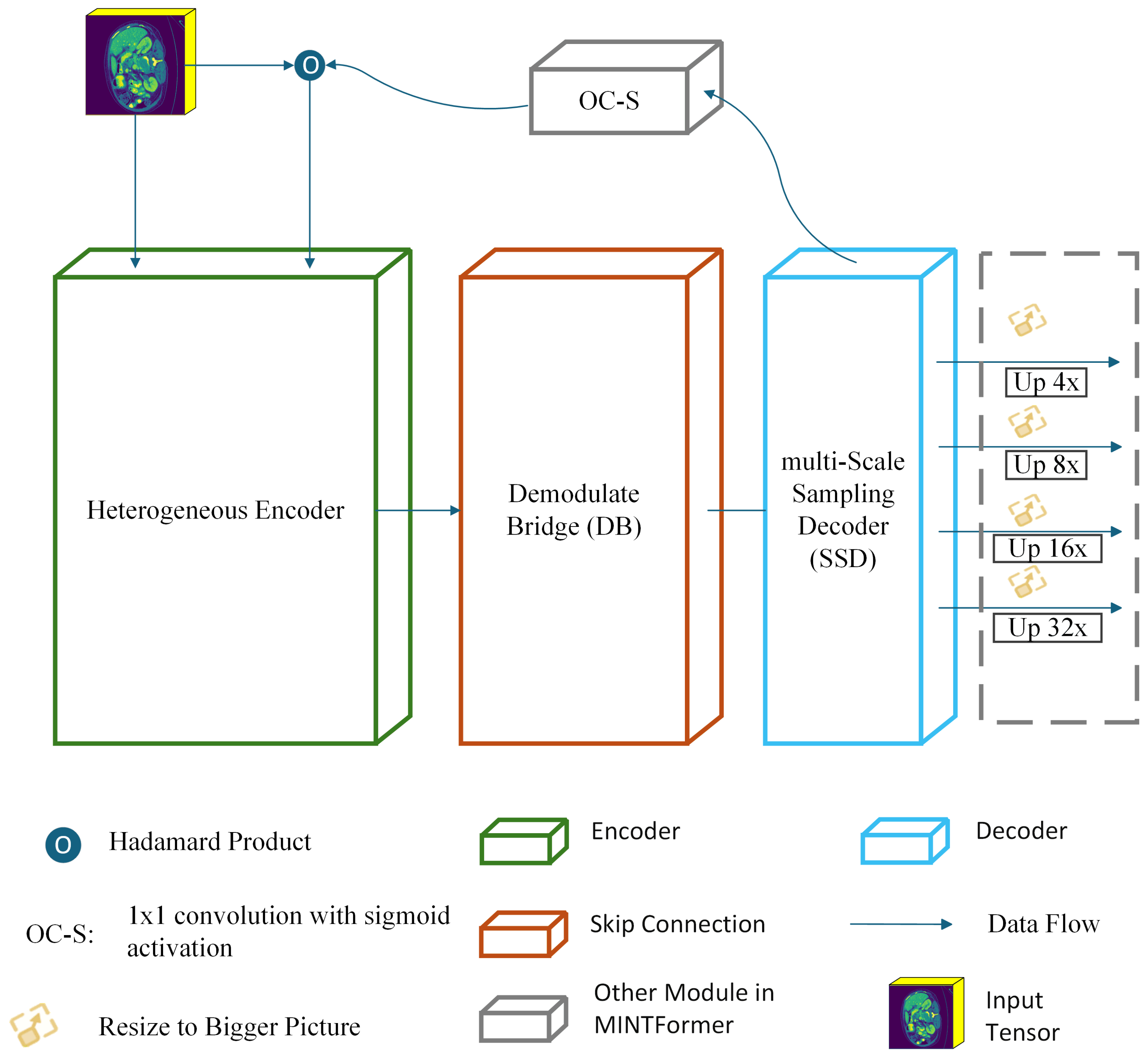
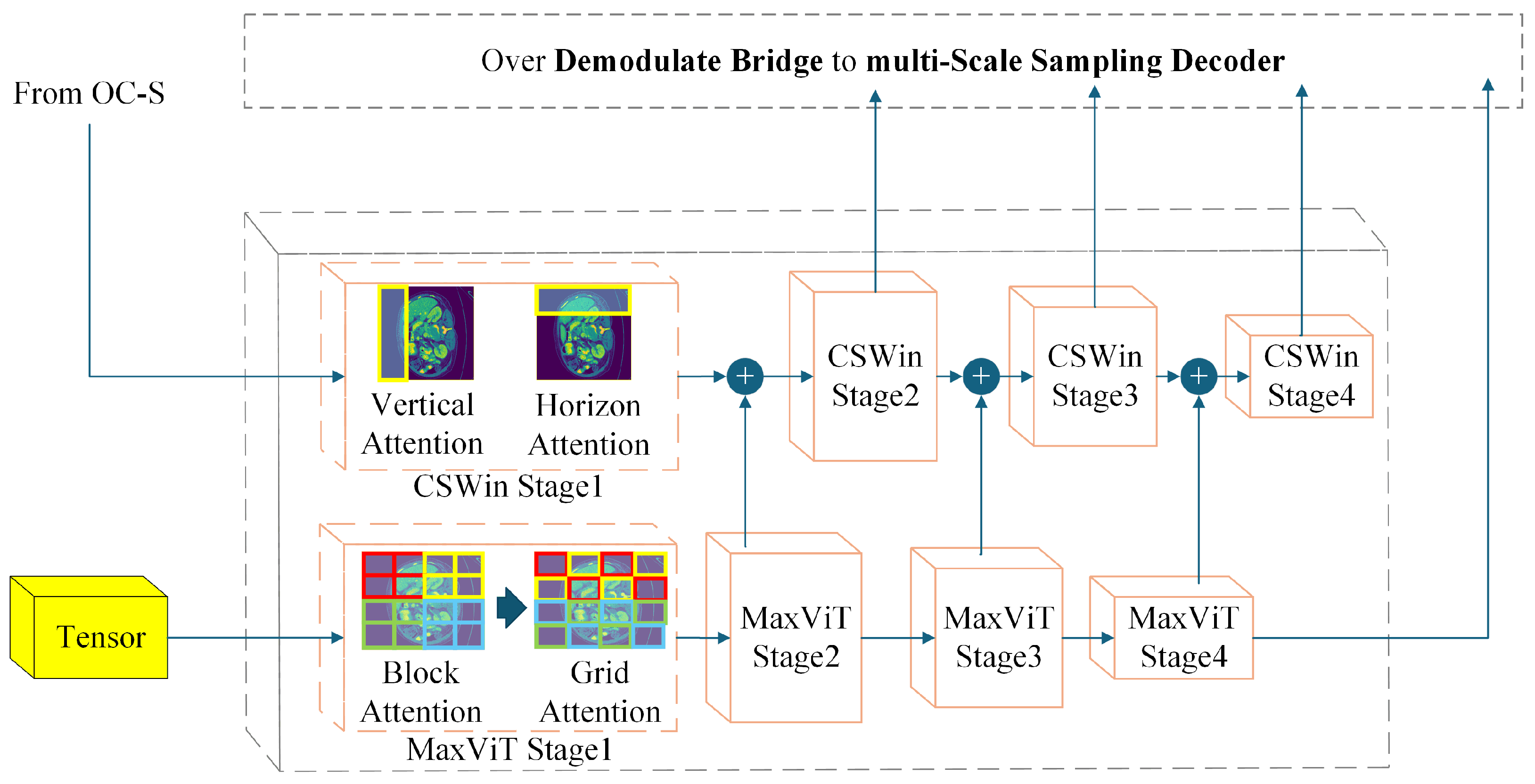
The overall architecture of MINTFormer is illustrated in Figure 1. MINTFormer comprises a Heterogeneous encoder, a Demodulate Bridge, a multi-Scale Sampling Decoder, and an aggregation output head. In MINTFormer, the MaxViT module initially performs the encoding operation. For any input feature map with a fixed dimension, the MaxViT stem stage encodes the feature map into patches using a convolution operation with a kernel size of and a stride of 4. The resulting patches then enter the MaxViT encoder for further encoding. The feature map produced by MaxViT is subsequently filtered by the Demodulate Bridge to eliminate redundant information. The filtered feature map is then fed into the multi-Scale Sampling Decoder for decoding. The resulting prediction map is scaled to the dimension of the feature map received by CSWin through the OC-S module and weighted with the feature map about to be input to the CSWin stem. Similarly, the feature map produced by CSWin is filtered by the Demodulate Bridge to eliminate redundant data. The feature maps produced by CSWin and MaxViT are then merged and decoded in the multi-Scale Sampling Decoder. Following the MERIT approach, the output of the multi-Scale Sampling Decoder is upsampled in the output head to generate the prediction map. The public announcement of MINTFormer is presented below.
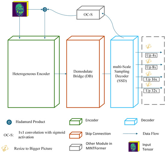
Figure 1.
MINTFormer framework diagram.
In Equation (1), denotes the output set of the feature map and , x represents the feature map, and y represents the final output of MINTFormer. and denote the MaxViT and CSWin components of the Heterogeneous encoder, respectively. represents the multi-Scale Sampling Decoder, denotes the Demodulate Bridge, and signifies upsampling the feature map to using bilinear interpolation.
3.1. Heterogeneous Encoder
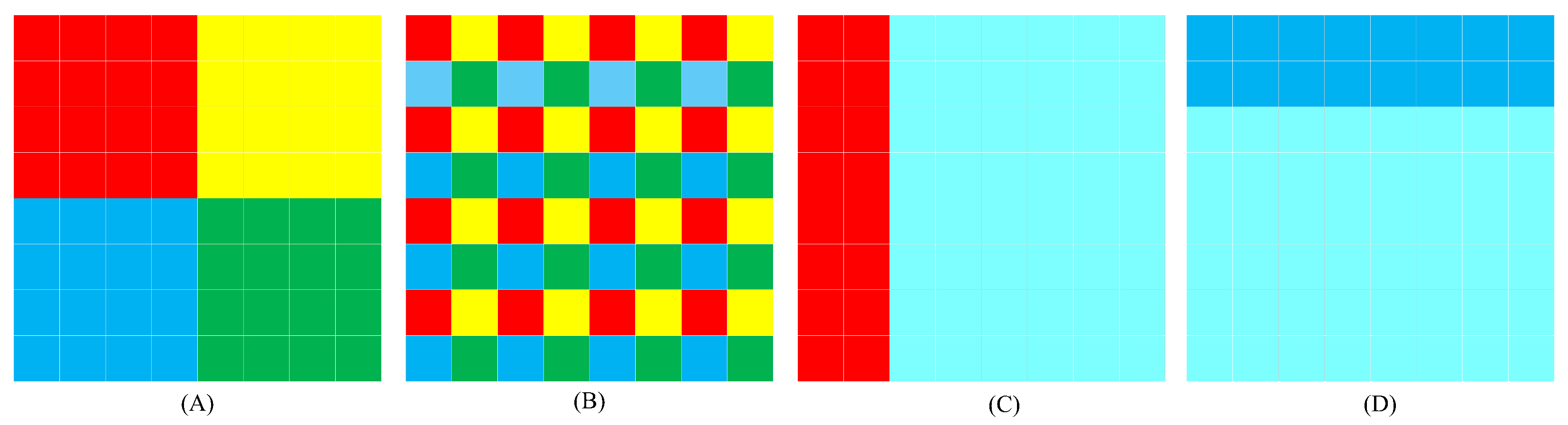
MaxViT employs a multi-axis attention mechanism to assign weights to feature maps, as illustrated in Figure 2A,B. Multi-axis attention can be divided into two distinct components: block attention and grid attention. Block attention involves partitioning the feature map into a series of non-overlapping windows, with self-attention calculations conducted within each distinct window. In contrast, grid attention does not employ a fixed window size for the division of the feature map. For a feature map of dimensions , the grid attention mechanism uses an attention window of size , thereby converting the feature map dimension to . The combination of block attention and grid attention allows MaxViT to balance local and global information processing. Although MaxViT effectively captures local information through block attention, it is important to note that organs in the human body are not isolated; there is connective tissue between organs. MaxViT’s operation of segmenting the feature map into multiple patches causes it to overlook the information of the connective tissue. Therefore, the Heterogeneous encoder incorporates CSWin alongside MaxViT. Cross Shape Window attention mechanism of CSWin is illustrated in Figure 2C,D: CSWin’s self-attention organizes the attention into horizontal and vertical stripes, enabling CSWin to effectively supplement the missing connective tissue information in MaxViT.
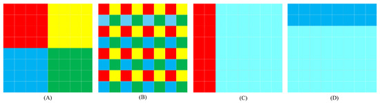
Figure 2.
(A) Block attention mechanism of MaxViT. (B) Grid attention mechanism of MaxViT. (C) Vertical attention mechanism of CSWin. (D) Horizontal attention mechanism of CSWin.
Figure 3 depicts the structure of the Heterogeneous encoder. Heterogeneous encoder is divided into two parts: the MaxViT encoder and the CSWin encoder. The feature map is first processed by MaxViT, after which the weighted feature map is processed by the decoder and weighted into the feature map about to be input to CSWin. Finally, CSWin weights the feature map, and the feature map output by CSWin also needs to enter the decoder. The workflow of the Heterogeneous encoder is shown in Equation (2).
x is feature map with a size of , represents the feature map output by , ⊙ the feature map with a size of represents the Huffman dot product, is feature map output by .
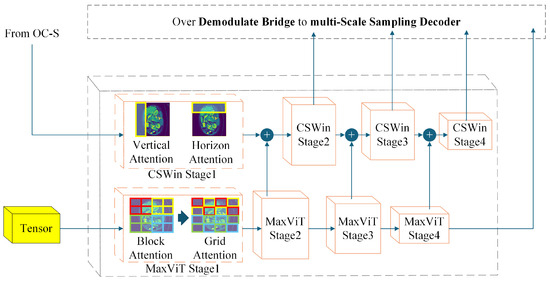
Figure 3.
Heterogeneous encoder structure diagram.
3.1.1. MaxViT Block
Figure 4 illustrates the internal structure of the MaxViT block. The MaxViT block comprises three fundamental components: MBConv, block attention, and grid attention. Initially, the feature map is processed by MBConv, which incorporates a squeeze-excitation (SE) module. Additionally, MBConv includes a depthwise convolution, which can be regarded as a form of conditional position encoding, thereby eliminating the necessity for explicit position encoding operations in . Following MBConv, the feature map undergoes block attention to extract local information. Finally, the feature map is subjected to grid attention to extract global information. The formula of the MaxViT block is provided in Equation (3).
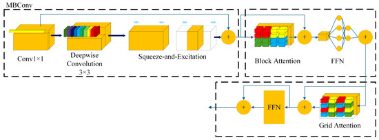
Figure 4.
Internal structure of a MaxViT block.
Let x represent the feature map, and denote the convolution operation with a kernel size of . and represent block attention and grid attention, respectively. denotes the feedforward network with residual connection. The feature maps , , and represent the feature map x after processing via MBConv, block attention, and grid attention, respectively. The symbol ⊕ represents matrix addition.
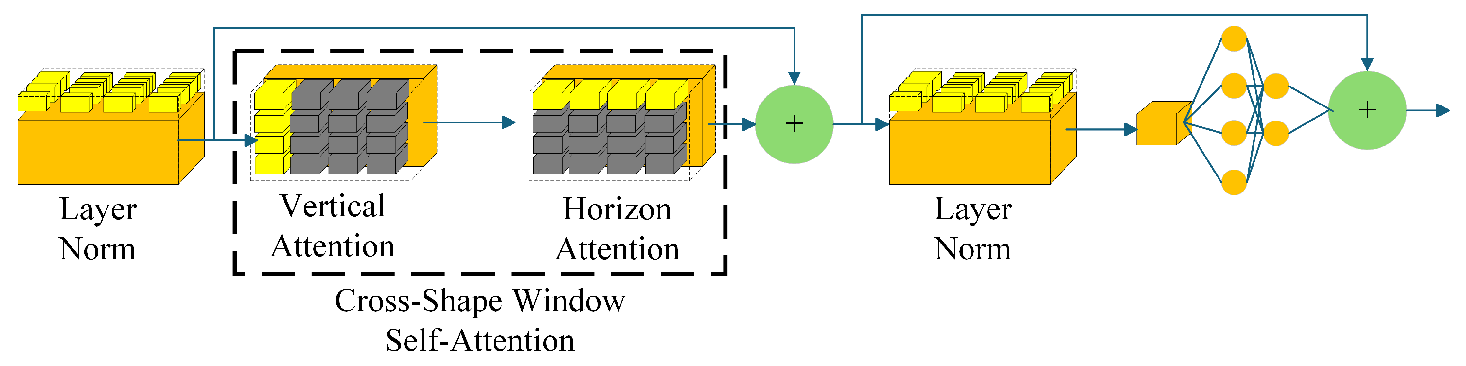
3.1.2. CSWin Block
The internal structure of the CSWin block is shown in Figure 5. CSWin block can supplement the connective tissue information between organs for the feature map. The feature map enters the CSWin block, where it is first normalized by , then weighted by cross-shape window self-attention (), and finally organized by the multi-layer perceptron (). The working process of the CSWin block is represented by Equation (4).
Figure 5.
Internal structure of a CSWin block.
3.2. Demodulate Bridge
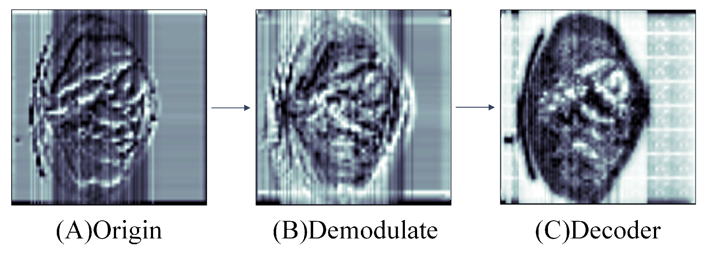
The process of the encoder processing the feature map can be regarded as a modulation process. The Demodulate Bridge serves to filter out any irrelevant information present in the feature map while simultaneously retaining the necessary feature information. Due to the constraints inherent in the encoder’s encoding methodology, the feature map generated by the encoder will encompass redundant texture data corresponding to the encoder’s encoding approach. It is thus necessary to filter the redundant texture information at this stage, a process analogous to demodulation. Figure 6 illustrates the effect of the Demodulate Bridge in filtering redundant information. Figure 6A depicts the original feature map, which exhibits numerous redundant black stripes. In contrast, Figure 6B shows that the Demodulate Bridge has significantly reduced the black numerical stripes, thereby enhancing the clarity and detail of the feature map. The reduction of redundant information facilitates the accurate restoration of the various details of the feature map by the decoder.

Figure 6.
Feature map demodulation effect diagram: (A) feature map output by the decoder; (B) feature map with redundant information filtered by Demodulate Bridge; (C) feature map upsampled at the same stage.
The output feature maps from all four stages in the encoder are provided to the Demodulate Bridge for the purpose of undergoing a demodulation operation. In the case of feature maps with a data dimension of , Demodulate Bridge will perform a convolution operation on the feature maps using a convolution kernel size of and a padding size of . Particular parameter settings of the Demodulate Bridge will be elucidated in the experimental section. Internal structure of Demodulate Bridge is illustrated in Figure 7, and the formula representation of the Demodulate Bridge is shown in Equation (5).
represents the feature map output from the heterogeneous decoder at stage i, represents the 2D convolution operation at stage i with convolution kernel size and padding size . The organized feature map is fed into the multiscale sampling encoder for the up-sampling operation.
Figure 7.
Internal structure diagram of Demodulate Bridge.
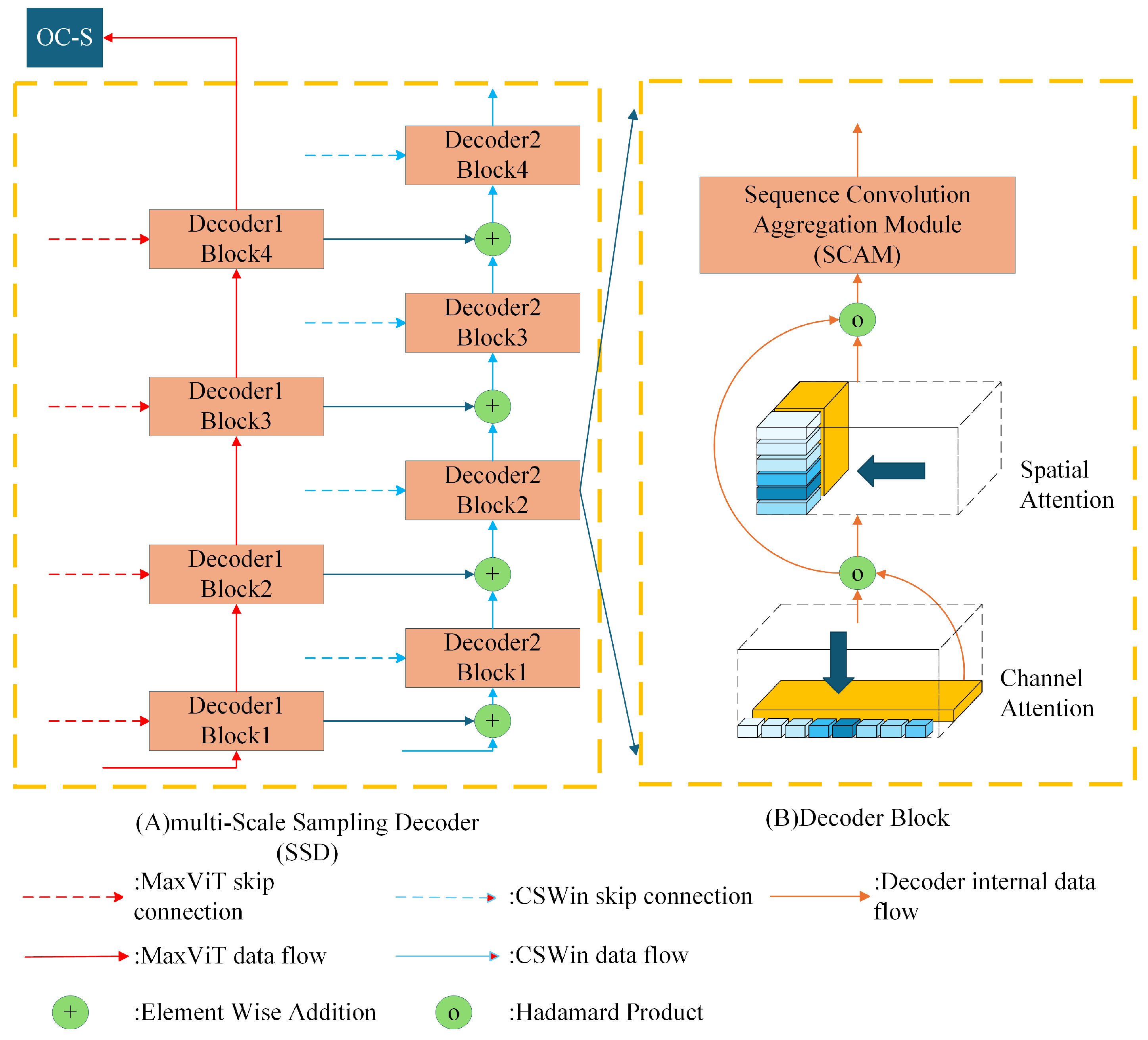
3.3. Multi-Scale Sampling Decoder
The multi-Scale Sampling Decoder (SSD) is analogous to the Heterogeneous encoder and comprises four stages, each employing bilinear interpolation for upsampling between stages. The structure of the multi-scale adoption decoder is illustrated in Figure 8A. SSD consists of two distinct components. In the initial stage, the output of MaxViT is input into Decoder 1 for decoding purposes. Subsequently, the feature map generated by Decoder 1 is fed into the OC-S module, which weights the feature map that is about to be input into CSWin. In the second part, the output of CSWin is input into Decoder 2. Decoder 2 accepts the outputs from CSWin, MaxViT, and Decoder 1, and fuses these three feature maps during the decoding stage. The fused feature map is then output to the classification header. The formula representation of SSD is shown in Equation (6).
Figure 8.
Multi-Scale Sampling Decoder structure diagram.
In this context, denotes a collection of feature maps, represents a feature map of the ith stage output by MaxViT, represents a feature map of the ith stage output by Decoder 1, represents a feature map of the ith stage output by CSWin, and represents a feature map of the ith stage output by Decoder 2.
Decoder1 accepts as input the feature map output by MaxViT, which is expressed as shown in Equation (7).
denotes the Decoder1 block of in i stage, denotes the feature map output by MaxViT of the current stage, denotes the feature map output by , represents the feature map of the current stage output by Decoder 1, and the feature map generated by the final stage of Decoder 1 enters the to generate the weighted map .
Decoder 2 accepts as input the feature map output by Decoder 1 with the feature map output by CSWin, which is expressed as shown in Equation (8).
where denotes the Decoder 2 block of the ith stage, denotes the feature map output by CSWin for the current stage, denotes the feature map output by , denotes the feature map output by Decoder 2 for the current stage, and denotes the feature map output by Decoder 1 for the ith stage.
is responsible for processing the MaxViT-generated feature map x into a weighted map to weight the coding work for CSWin. represented by the formula as shown in Equation (9).
where y represents the weighted map, x represents the feature map of the input , represents the maximum pooling operation, and represents the layer normalization.
Decoder 1 and Decoder 2 have the same internal structure for their decoder blocks; the internal structure of the decoder block is shown in Figure 8B. In this structure, the feature map is first weighted by channel attention [44], followed by spatial attention [45], and finally enters the sequence convolution aggregation module to extract multi-scale organ features. The formula representation of the decoder block is shown as follows:
where x is the feature map of the input decoder block, y is the output of the decoder block, represents the channel attention, represents the spatial attention, represents the sequence convolutional aggregation module, and ⊙ represents the Huffman dot product. Next in this manuscript, the three sub-modules , and are explained.
3.3.1. Channel Attention
The task of channel attention is to decide which of the feature maps are to be attended to and to enhance those feature maps. The formulaic representation of channel attention is shown in Equation (11).
where x represents the feature map of the input channel attention and y represents its output. represents a convolution operation having a convolution kernel that organizes the information of the feature map in the channel dimension. represents the Sigmoid activation function and ⊙ represents the Huffman dot product.
3.3.2. Spatial Attention
The task of spatial attention is to decide which part of the feature map needs to be enhanced in order to enrich the spatial context information within the feature map. The definition of spatial attention is shown in Equation (12).
where represents a convolution operation having a convolution kernel of size that organizes the information of the feature map in the spatial dimension.
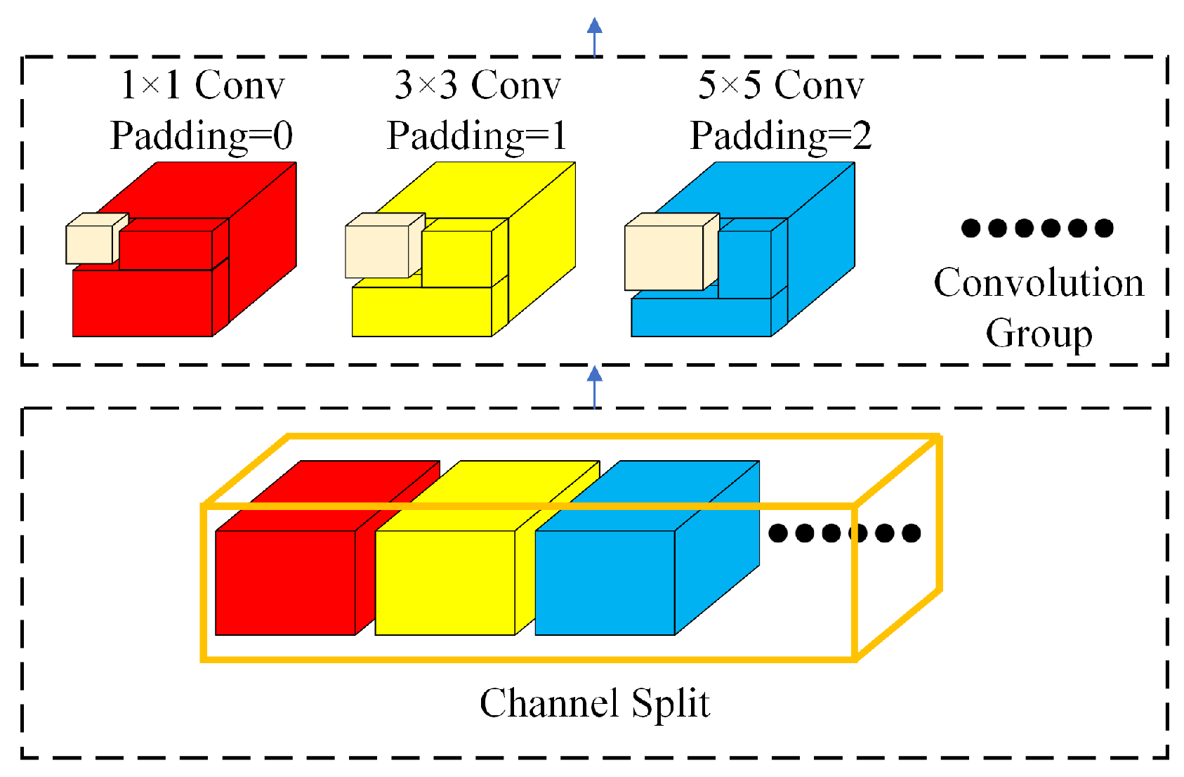
3.3.3. Sequence Convolution Aggregation Module
IDConv, as part of the TransXNet, divides the feature maps into smaller units along the channel dimension. For each of these sub-maps, a distinct convolution operation is applied, allowing the model to capture detailed local information while maintaining a sufficiently expansive perceptual field of view. However, given that the dimensionality of the feature maps at each stage differs, it is not appropriate for IDConv to set the same convolution combination for all feature maps at all stages. It is necessary to dynamically modify the convolution combination for feature maps of varying dimensions. The structure of the sequence convolutional aggregation module is illustrated in Figure 9. Upon entering the sequence convolutional aggregation module, the feature map is sliced into multiple sub-maps along the channel dimension, with each sub-map scanned by its corresponding convolutional kernel. The formula representation of the sequential convolutional aggregation module is shown in Equation (13).
where x represents the feature map of the input sequence convolutional aggregation module, represents the set of sub-maps sliced by x to N part, represents the operation of channel slicing, and represents the processing of the convolution group.
Figure 9.
Structure of the sequential convolutional aggregation module.
4. Experiments
MINTFormer is built using the PyTorch 2.7.1 framework for training and testing tasks on the Nvidia GeForce RTX 4080 GPU platform (Colorful, Beijing, China). To accelerate the convergence speed of MINTFormer during training, we introduce pre-training weights based on ImageNet-1k for MaxViT, which handles feature maps with dimensions of , and pre-training weights based on ImageNet-1k for CSWin, which accepts feature maps. The batch size is set to 14, the training duration was 300 epochs, and MINTFormer uses AdamW with a learning rate of and a weight decay of as the optimizer. This configuration enables MINTFormer to balance fast learning and stable convergence. This project is based on CASCADE for the design of the loss function, which is expressed in the following formula:
where represent the feature maps output from the four stages in MINTFormer, and represent the four hyperparameters. This training strategy can balance the weights between deep information and shallow features, so that MINTFormer can efficiently utilize the abstract semantic information in the deep features.
4.1. Dataset
This project classifies the datasets utilized in the experiments into two categories: multi-scale organ information datasets and single-scale organ information datasets. A multi-scale organ information dataset is defined as a collection of samples containing multiple labels, requiring the model to label multiple objects within a single feature map. For instance, in the ACDC dataset, the network must accurately label the left ventricle, the right ventricle, and the myocardium in a single feature map. The objective of the multi-scale organ information dataset is to assess the model’s capacity for generalization. This is because the network must learn the characteristics of multiple organs within the multi-scale organ information dataset and ensure that the labeled regions do not conflict with one another. In contrast, a single-scale organ information dataset comprises a single organ within a feature map, necessitating that the model discern the organ region from the background region. As the single-scale organ information dataset has a single label, it is possible to achieve higher test scores if the model can accurately delineate the organ’s boundaries. Therefore, the single-scale organ information dataset places significant demands on the model’s ability to capture details. In this project, the multi-scale organ information datasets employed for testing purposes are Synapse [7] and ACDC [46]. The single-scale organ information datasets utilized for testing are skin lesion segmentation datasets (ISIC2017 [47], ISIC2018 [48] with [49]) and Kvasir-SEG [50].
4.1.1. Synapse Dataset
Synapse is a multi-organ segmentation dataset. The Synapse dataset consists of 30 abdominal CT scans and 3779 axial abdominal clinical CT images, each CT volume consists of 85–98, -sized pixel slices with a voxel spatial resolution of mm3. Eight abdominal organs are present within the dataset (aorta, gallbladder, left kidney, right kidney, liver, pancreas, spleen, and stomach). The dataset was randomly divided into 18 scanned images for training and 12 scanned images for testing [51]. To facilitate the training, the Synapse dataset processed by TransUnet was used for this experiment.
4.1.2. ACDC Dataset
The ACDC dataset consists of 100 MRI scans collected from different patients, each labeling three organs: the left ventricle (LV), the right ventricle (RV), and the myocardium (MYO). The ACDC dataset includes cardiac findings from different patients acquired with an MRI scanner. MR images were acquired under breath-hold and a series of short-axis slices covering the heart from the base of the left ventricle to the apex, with slice thicknesses ranging from 5 to 8 mm. The spatial resolution in the short-axis plane was (0.83–1.75) mm2/pixel. Each patient scan was manually annotated with the true conditions of the left ventricle (LV), right ventricle (RV), and myocardium (MYO). The ACDC dataset was randomly segmented with 70 training cases (1930 axial slices), 10 cases for validation, and 20 cases for testing. Consistent with previous work [52], the Dice coefficient is used in this study to evaluate the performance of MINTFormer.
4.1.3. Kvasir-SEG Dataset
Kvasir-SEG is an endoscopic dataset for pixel-level segmentation of colorectal polyps. Kvasir-SEG includes 1000 gastrointestinal polyp images and their corresponding segmentation masks, all annotated and verified by experienced gastroenterologists. The dataset provides a training and validation split in a ratio of 880:120 to fairly compare various models. This dataset aims to promote research and innovation in the segmentation, detection, localization, and classification of colorectal polyps. Following previous practices [53], we use 70 cases for training, 10 cases for validation, and 20 cases for testing, and employ the Dice coefficient to evaluate the performance of MINTFormer.
4.1.4. Skin Lesion Segmentation Datasets
The datasets utilized for the segmentation of skin lesions encompass the ISIC2017, ISIC2018, and datasets. The ISIC dataset comprises a substantial number of dermatoscopic images, encompassing a diverse range of skin lesions. In accordance with the parameters established for HiFormer, the ISIC2017 dataset was divided into the following training, validation, and testing sets: 1400 images for training, 200 images for validation, and 400 images for testing. The training set consisted of 1815 images. In the ISIC2018 dataset, 259 images are designated for validation, while 520 images are designated for testing. In the dataset, 80 images are designated for training, 20 images are designated for validation, and 20 images are designated for testing. The dataset was divided into three subsets: training (80 images), validation (20 images), and testing (100 images). The performance of the skin lesion segmentation task was evaluated using four metrics: average Dice coefficient, sensitivity (SE), specificity (SP), and accuracy (ACC).
4.2. Evaluation Metrics
4.2.1. Dice
In the context of medical imaging competitions, the Dice coefficient is the most frequently utilized metric. It is an ensemble similarity metric, typically employed to quantify the similarity between two samples, with a value domain of . Its applications extend to image segmentation in medical imaging, where the optimal outcome is a segmentation value of 1, and the least favorable result is a segmentation value of 0. The Dice coefficient is calculated according to the following Equation (15): represents the set of points predicted by the network, and represents the set of true values.
4.2.2. HD95
This experiment employs the 95% Hausdorff distance(HD95) to quantify the extent of overlap between the boundaries. HD95 determines the distance between two sets, with smaller values indicating greater similarity between the two. The formula for HD95 is as follows:
In Equation (16), stands for two point sets, stands for the distance between two points sets of X and Y, stands for the distance between the point set Y and point set X.
4.3. Result
4.3.1. Experimental Results of Multi-Scale Organ Information Dataset
Synapse Dataset
As illustrated in Table 1, we employed the Dice with HD95 to evaluate the performance of each model within the Synapse dataset. Subsequently, the Dice and HD95 mean columns are followed by the Dice for different organs, where GB represents the gallbladder, KL and KR are the left and right kidneys, PC is the pancreas, SP is the spleen, and SM is the stomach. MINTFormer achieves an excellent result in Synapse, with the best Dice and lowest HD95. TransCascade and Missformer exhibited a 2.06% and 2.78% improvement in Dice, respectively, and a 3.31 and 4.17 improvement in HD95. Concurrently, MINTFormer also demonstrated the most optimal Dice for the gallbladder, left and right kidneys, pancreas, and stomach. This illustrates that MINTFormer is capable of effectively capturing the multi-scale information of both large and small organs.

Table 1.
Synapse experiment results, best result is highlight in red, and the second best result is highlight in blue, ↑ indicates higher values are better, ↓ indicates lower values are better.
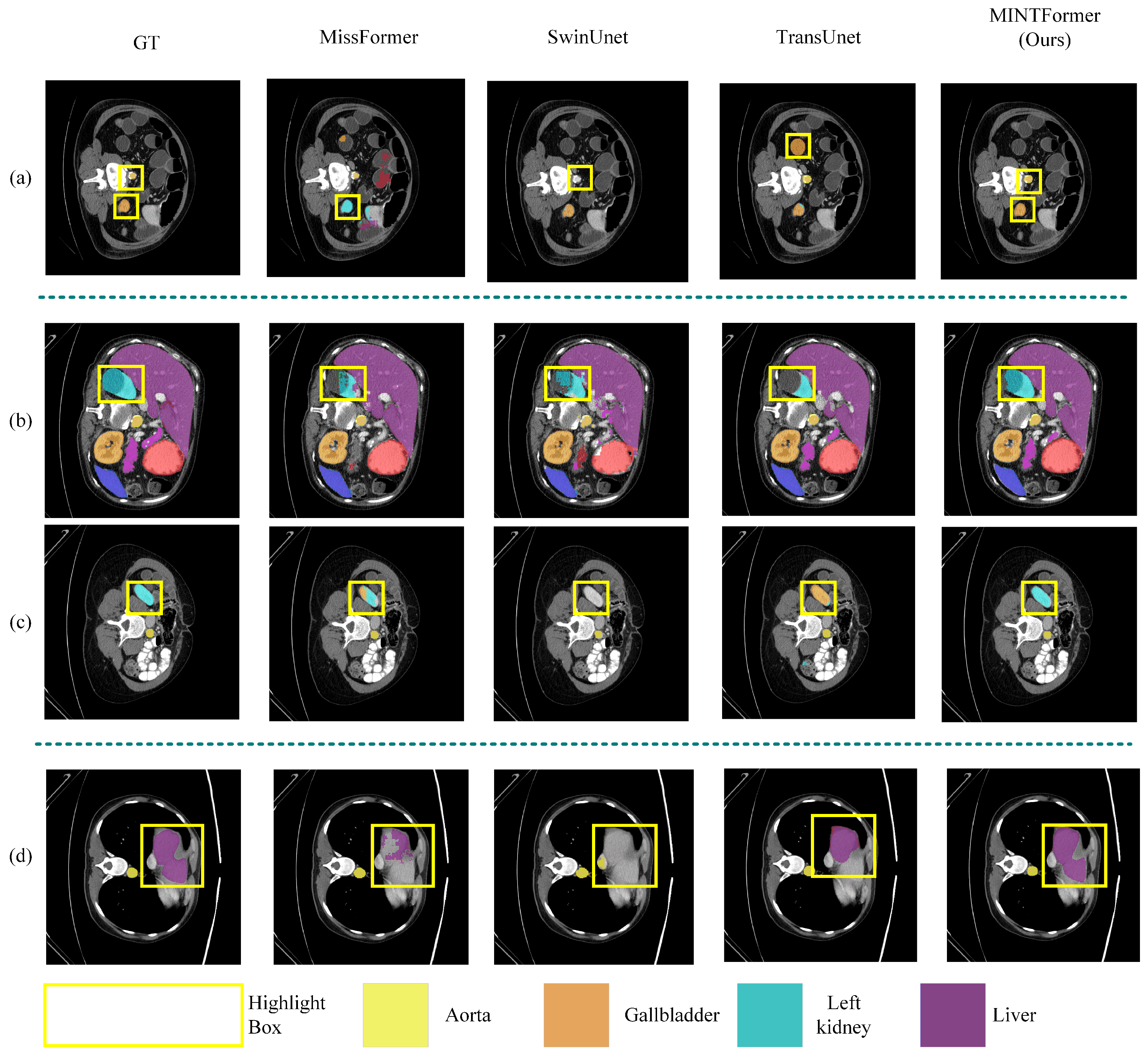
To facilitate a more intuitive evaluation of the segmentation performance of MINTFormer, we present the segmentation results of the Synapse dataset across different models. Figure 10 illustrates the segmentation outcomes of Synapse in MINTFormer, Missformer, SwinUnet, and TransUnet.

Figure 10.
Depicts the segmentation results of eight abdominal organs (aorta, gallbladder, left kidney, right kidney, liver, pancreas, spleen, and stomach) in the Synapse dataset, employing a variety of models. (a) The location of small organs in the marked feature map that are easily overlooked by the model. (b,c) The location of medium-sized organs in the marked feature map that are challenging for the model to process, resulting in incomplete organ information. (d) The location of large organs in the marked feature map that are difficult for the model to decode and retain all the information.
As illustrated in Figure 10a, certain models exhibit deficiencies in accurately identifying minute objects within the segmentation process conducted on the Synapse dataset. The two labeled organs in Figure 10a are the gallbladder and the aorta. These organs occupy a relatively limited area of the feature map and are of a relatively small size. Upon examination of the highlighted regions, it becomes evident that other models have made erroneous predictions. For instance, Missformer incorrectly identifies the gallbladder as other types of organs, while SwinUnet mislabels the aorta. Additionally, TransUnet mislocalizes the aorta. However, MINTFormer is the only model that accurately predicts both organs, substantiating its exceptional capacity to discern intricate details and distinguish between relevant and irrelevant structures.
In Figure 10b the area encircled in yellow represents the left kidney. It is evident that MINTFormer has performed the most comprehensive segmentation of the left kidney. Missformer, TransUnet, and SwinUnet are unable to segment the relatively complete left kidney due to their inability to maintain multi-scale information. In Figure 10c the area highlighted in yellow represents the same left kidney, but it has been relocated to a different channel dimension, and the ground truth (GT) value of the left kidney has decreased accordingly. Missformer preserves some of the features of the left kidney due to the fixed-size convolution operation. However, SwinUnet does not employ a convolution operation to maintain sub-features during upsampling, resulting in its inability to detect the left kidney. MINTFormer successfully captures the multi-scale spatial information of the left kidney due to the utilization of a multi-Scale Sampling Decoder. This enables MINTFormer to correctly identify the left kidney across different channel dimensions.
In Figure 10d the organ identified in the center of the line is the liver. Missformer is capable of partially restoring the segmentation map of the liver due to the fixed-size convolution operation. However, the convolution kernel of Missformer is insufficiently sized, resulting in its receptive field failing to encompass the entirety of the liver. Consequently, Missformer is unable to achieve a complete restoration of the liver. SwinUnet does not employ multi-scale convolutions, leading to a significant discrepancy between the restored liver and the original label. In contrast, MINTFormer utilizes convolution groups capable of capturing multi-scale information in the feature map through convolution kernels of varying sizes, enabling the complete restoration of the liver segmentation map.
Result of ACDC
Table 2 presents the experimental findings for MINTFormer on the ACDC dataset. RV represents Dice coefficient obtained by the model for the right ventricle, MYO represents Dice coefficient obtained by the model for the myocardium, and LV represents the left ventricle. It can be seen that MINTFormer achieved the best results in terms of the average Dice coefficient, in both LV and RV, and ranked second in MYO. This demonstrates that MINTFormer has good generalization and robustness.
Table 2.
Experimental results on ACDC dataset and Kvasir-SEG dataset, best result is highlight in red, and the second best result is highlight in blue.
4.4. Experimental Results of Single-Scale Organ Information Dataset
4.4.1. Experimental Results on the Kvasir-SEG Dataset
Table 2 presents the performance of different models on the Kvasir-SEG dataset. It can be observed that MINTFormer achieved the best results compared to other models. Specifically, MINTFormer improved the average Dice coefficient by 1.04% and 10.44% compared to KDAS3 and U-Net++, respectively. This indicates that MINTFormer can accurately capture the boundary details of feature maps even in single-scale organ information datasets, rather than causing confusion between the two backbone networks.
4.4.2. Experimental Results on Skin Lesion Segmentation Datasets
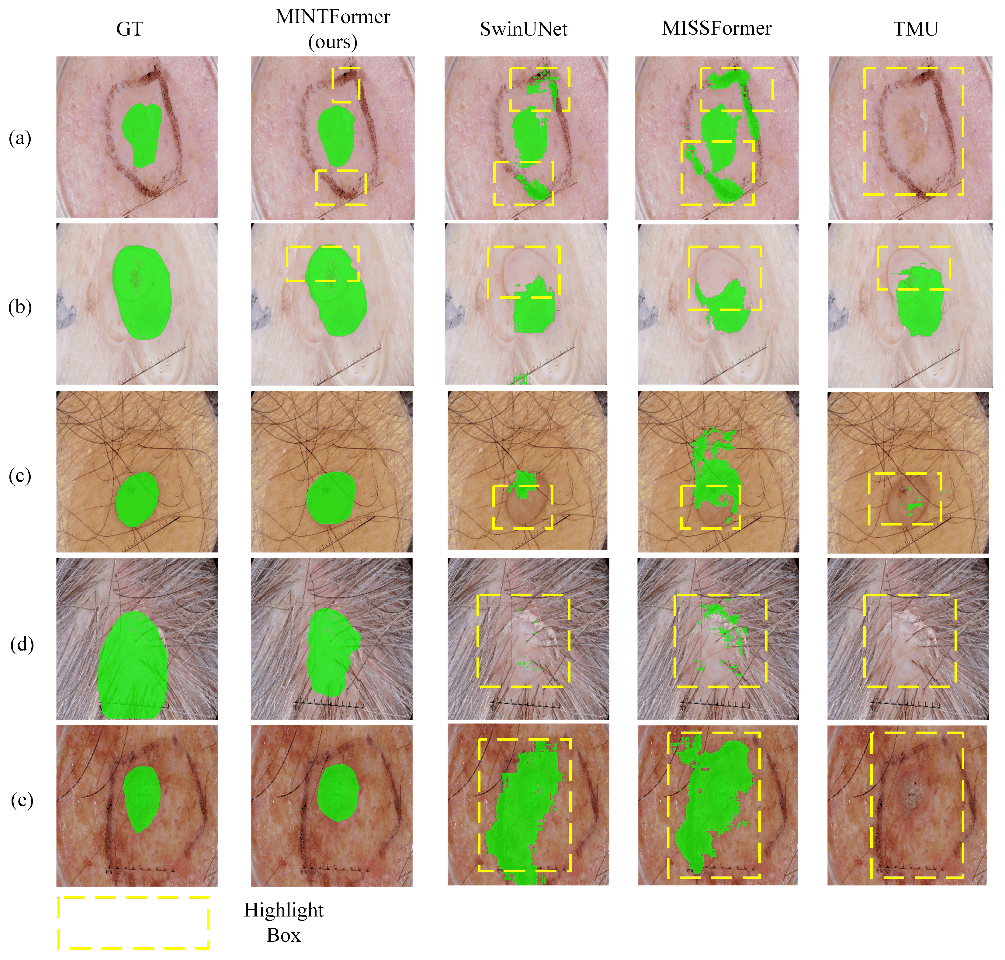
Table 3 presents the experimental results of MINTFormer and other advanced models on skin lesion segmentation datasets. MINTFormer achieved the best performance in terms of the Dice coefficient, reflecting its strong segmentation capability to accurately delineate skin lesion areas. Figure 11 shows the visual comparison of lesion segmentation results on the ISIC2017 dataset between MINTFormer and other advanced models. In Figure 11a,b, the background of the lesion areas is simple, making it easier for the models to capture the features of the lesion areas. Observing the highlighted regions, although most models can mark the approximate location of the lesion areas, not all models can capture the boundary details of the lesion areas. In Figure 11a, MINTFormer not only accurately marks the lesion areas but also avoids mislabeling the surrounding interference information as lesion areas. In contrast, SwinUnet and Missformer incorrectly label the interference information. In Figure 11b, all models can mark the approximate location of the lesion areas, but only MINTFormer can more accurately restore the shape of the lesion areas. In Figure 11c–e, the background of the lesion areas becomes more complex, which further tests the models’ ability to filter redundant information. It can be seen that in Figure 11c–e, except for MINTFormer, other models struggle to mark the location of the lesion areas accurately. The marked lesion areas by other models significantly deviate from the ground truth.
Table 3.
Experimental results of MINTFormer on skin lesion segmentation datasets, best result is highlight in red, and the second best result is highlight in blue, ↑ indicates higher values are better.
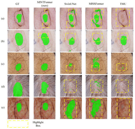
Figure 11.
Visualization of Segmentation Results of MINTFormer and Other Advanced Models on the ISIC2017 Dataset. (a,b) show the models’ ability to segment skin lesion areas in simple backgrounds. (c–e) show the models’ ability to segment lesion areas in complex backgrounds.
4.5. Ablation Study
In this section, we conduct ablation experiments on MINTFormer using the Synapse dataset. Specifically, we explore the selection of the maximum convolution kernel in the convolution group of the decoder, the choice of convolution parameters in the Demodulate Bridge, and the combination of hyperparameters in the loss function.
4.5.1. Selection of the Maximum Convolution Kernel in the Convolution Group of the Decoder
In SSD, the default maximum convolution kernel (MaxConvKernel) in the convolution group is set to half the side length of the feature map. We conducted comparative experiments using one-quarter, three-quarters, and the full side length of the feature map as the maximum convolution kernel in the convolution group to explore the optimal parameters for the maximum convolution kernel. As shown in Table 4, H represents the side length of the feature map. When using as the maximum convolution kernel size, smaller convolution kernels occupy a larger proportion in the convolution group, allowing SSD to capture more information about small organs. Consequently, with , MINTFormer achieves higher Dice scores for small organs such as the aorta, gallbladder, and pancreas. When using H as the maximum convolution kernel in the convolution group, larger convolution kernels occupy a larger proportion, resulting in MINTFormer achieving better Dice scores for large organs such as the liver. However, this also leads to a loss of information about small organs. Overall, is a more balanced choice.
Table 4.
Impact of the Maximum Convolution Kernel in the Convolution Group on MINTFormer’s experimental results on the Synapse dataset, best result is highlight in red, ↑ indicates higher values are better.
4.5.2. Selection of Convolution Parameters in the Demodulate Bridge
The data dimensions of feature maps at different stages vary. It is essential to select appropriate convolution kernels for feature maps of different sizes to adequately filter out redundant information within the feature maps. As shown in Table 5, it is necessary to use the Demodulate Bridge to filter out redundant information in the feature maps. Plan 4, which did not use any convolution operations to filter information in the feature maps, achieved the worst results. Plan 2 used overly large convolution kernels to filter redundant information. Plan 3 used convolution kernels of the same size for feature maps at all stages, resulting in the second-best performance. In summary, using convolution kernels of sizes 7, 5, 3, and 1 to filter feature maps at the four stages is a balanced choice.
Table 5.
Impact of convolution parameters in the Demodulate Bridge on MINTFormer’s experimental results on the Synapse dataset, ↑ indicates higher values are better. ↓ indicates lower values are better.
4.6. Efficiency Analysis
To comprehensively evaluate the advantages and disadvantages of MINTFormer, we conducted a performance analysis using the ISIC2017 dataset on the Nvidia A100 platform (Nvidia, Beijing, China). As shown in Table 6, the Large model of MINTFormer achieved the best results but also occupied the most parameters, with 122.12 M parameters that require an Nvidia 4080 (Colorful, Beijing, China) or higher level compute card to operate. The Middle model, which can be run on an Nvidia 4070 or equivalent mid-level compute card, achieved sub-optimal results. The Small model requires an Nvidia 4060 or equivalent compute card and has the lowest performance. In our clinical setting, the inference hardware used is the Nvidia 4080 compute card, which can fully support the inference tasks of MINTFormer’s Large model.
Table 6.
Result of efficiency analysis, best result is highlight in red, ↑ indicates higher values are better, M stands for million and G stands for billion.
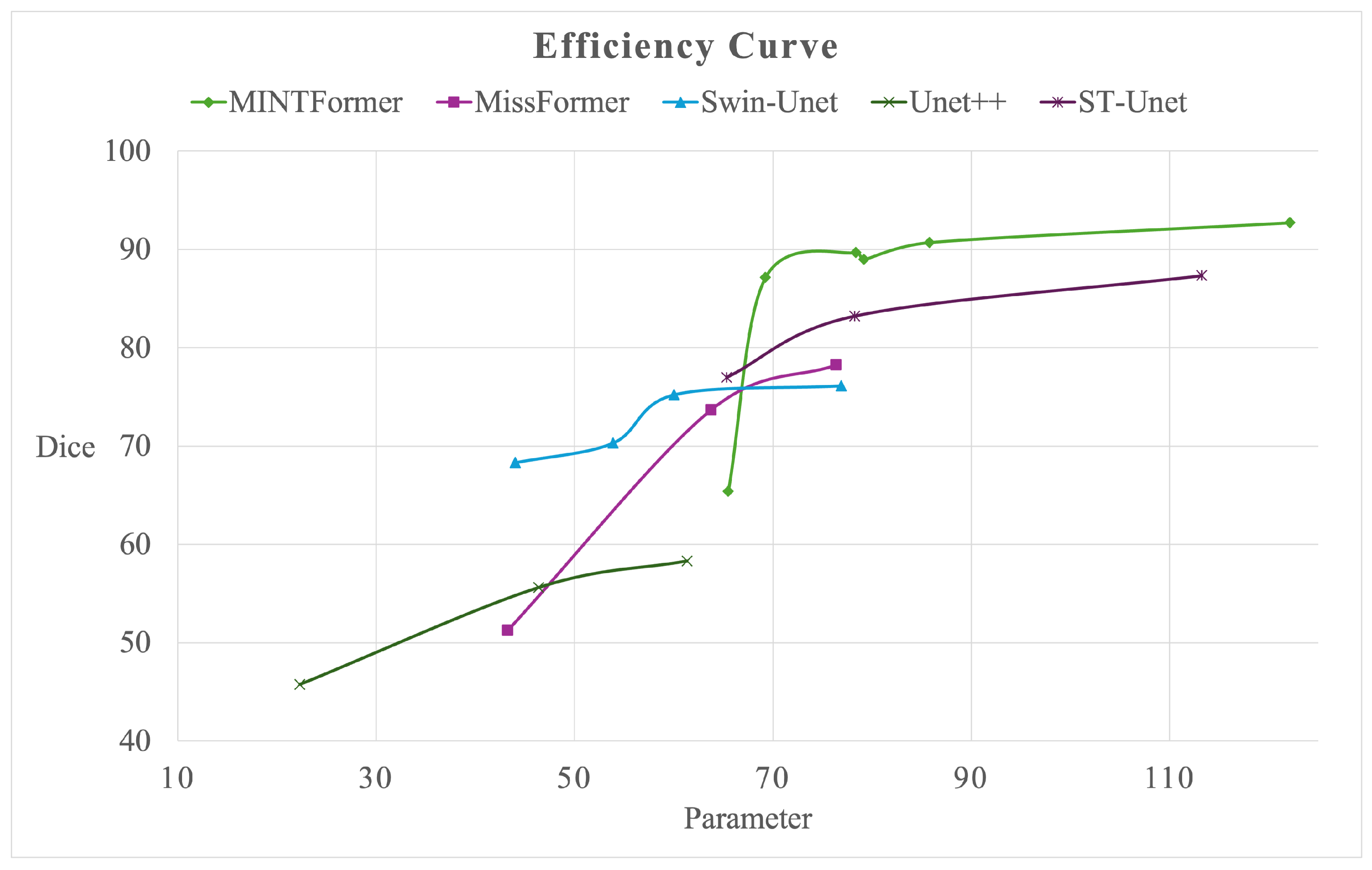
Furthermore, we plotted the energy efficiency curves for MINTFormer, using the ISIC2017 dataset for comparison with advanced models such as MissFormer [31], Swin-Unet [35], Unet++ [29], and ST-Unet [68]. As shown in Figure 12, MINTFormer’s energy efficiency curves for the middle model scale (parameter range of 70–90 M) and large model scale (parameters over 90 M) are superior to those of other advanced models. However, in the case of a smaller model scale (parameters less than 70 M), it is inferior to other models. This indicates that MINTFormer possesses strong information-capturing capabilities but lacks in lightweighting work.
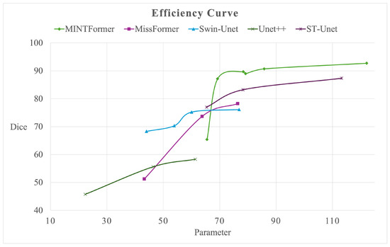
Figure 12.
Efficiency curve of MINTFormer.
4.7. Discussion
In MINTFormer, we conducted experiments on two different types of datasets: multi-scale organ information datasets (Synapse and ACDC) and single-scale organ information datasets (Kvasir-SEG, ISIC2017, ISIC2018, and ). The experimental results indicate that MINTFormer exhibits excellent performance across all types of datasets.
Specifically, CSWin’s cross-window attention mechanism organizes attention in horizontal and vertical stripe patterns, enabling efficient capture of connective tissue information between organs. Benefiting from CSWin’s capability to model long-range dependencies, it effectively addresses the issue of patch boundary discontinuities in traditional Transformer-based segmentation models. Meanwhile, MaxViT’s multi-axis attention mechanism demonstrates outstanding performance in balancing local details with global semantics through the synergistic interaction of grid attention and block attention. Block attention divides feature maps into non-overlapping windows to extract local information, while grid attention aggregates global context through dynamic windows. The collaborative effect of Heterogeneous Encoders is particularly prominent in multi-scale organ segmentation tasks. On the Synapse dataset, MINTFormer achieves an average Dice coefficient of 84.74%, representing a 2.06% improvement over TransCASCADE, while the HD95 metric decreases by 3.31. This indicates that the heterogeneous encoders not only enhance semantic integrity for large organs (e.g., liver, Dice 95.38%) but also significantly improve detail capture for small organs (e.g., pancreas, Dice 69.72%). The core mechanism lies in: CSWin complements structural relationships between organs through global context, while MaxViT refines organ boundary features via local attention. Through feature fusion in the Demodulate Bridge, they form a complementary segmentation paradigm of “global semantic guidance—local detail enhancement.”
However, MINTFormer still has some shortcomings. Compared to other models, MINTFormer consumes more computational resources and relies on pre-trained models of MaxViT and CSWin. Additionally, there is room for improvement in MINTFormer’s segmentation performance in certain extreme cases. As shown in Figure 11e, although MINTFormer can roughly mark the lesion location in complex backgrounds, it fails to fully capture the boundary details of the lesion. Therefore, making MINTFormer more lightweight and further enhancing its ability to capture detailed information are among our future research directions.
5. Conclusions
This study introduces the concept of a Heterogeneous encoder for the first time, integrating two different types of encoders to fully leverage their respective advantages. Additionally, this study designs a Demodulate Bridge to filter out redundant information in feature maps with low computational cost. In the decoder, we explore the ability of different convolution combinations to retain information about organs of various sizes. Based on the characteristics of the dataset labels, we classify medical datasets into multi-scale organ information datasets and single-scale organ information datasets. The experimental results demonstrate that MINTFormer maintains excellent performance across all types of datasets, indicating its great potential for further optimization and enhancement in deep learning applications for complex medical image segmentation tasks.
However, MINTFormer still has certain limitations. Efficiency analysis indicates that while MINTFormer achieves outstanding results with large-scale models, its performance remains inferior to that of other state-of-the-art models when used in medium or small-scale architectures. The reliance on large models imposes higher hardware requirements in clinical settings, thereby limiting MINTFormer’s generalizability. Therefore, future work will focus on lightweight optimizations to enhance its adaptability across diverse scenarios.
Additionally, to expand MINTFormer’s application scope, we have collected a substantial dataset of pancreatic cancer tissue slides. Upon completing the annotation process, we will evaluate MINTFormer’s potential for pancreatic cancer detection.
Author Contributions
Conceptualization, X.Q., C.D.; methodology, X.Q., C.D.; software, X.Q., C.D.; validation, X.Q.; formal analysis, C.D.; investigation, X.Q.; resources, X.Q.; data curation, X.Q.; writing—original draft preparation, C.D.; writing—review and editing, X.Q.; visualization, X.Q.; supervision, X.Q.; project administration, X.Q.; funding acquisition, X.Q. All authors have read and agreed to the published version of the manuscript.
Funding
This study was financially supported by STI2030-Major Projects (2021ZD0201900), Guangxi Key R&D Project (Grant no. AA22068057).
Institutional Review Board Statement
Not applicable.
Informed Consent Statement
Not applicable.
Data Availability Statement
Data available in a publicly accessible repository. This data can be found here: https://github.com/fdiskdc/mintformer (accessed on 11 June 2025).
Acknowledgments
Special thanks to Xiaosen Li (School of Artificial Intelligence, Guangxi Minzu University, Nanning, Guangxi, 530300, People’s Republic of China, e-mail: xiaosenforai@gmail.com) and Yuanyuan Li (School of Foreign Languages, Nanning Normal University, Nanning, Guangxi, 530100, People’s Republic of China, e-mail: 2765448846@qq.com) for guidance in this research.
Conflicts of Interest
The authors declare no conflicts of interest.
References
- Asgari Taghanaki, S.; Abhishek, K.; Cohen, J.P.; Cohen-Adad, J.; Hamarneh, G. Deep semantic segmentation of natural and medical images: A review. Artif. Intell. Rev. 2021, 54, 137–178. [Google Scholar] [CrossRef]
- Qureshi, I.; Yan, J.; Abbas, Q.; Shaheed, K.; Riaz, A.B.; Wahid, A.; Khan, M.W.J.; Szczuko, P. Medical image segmentation using deep semantic-based methods: A review of techniques, applications and emerging trends. Inf. Fusion 2023, 90, 316–352. [Google Scholar] [CrossRef]
- Wang, R.; Lei, T.; Cui, R.; Zhang, B.; Meng, H.; Nandi, A.K. Medical image segmentation using deep learning: A survey. IET Image Process. 2022, 16, 1243–1267. [Google Scholar] [CrossRef]
- Ronneberger, O.; Fischer, P.; Brox, T. U-net: Convolutional networks for biomedical image segmentation. In Proceedings of the Medical Image Computing and Computer-Assisted Intervention—MICCAI 2015: 18th International Conference, Munich, Germany, 5–9 October 2015; Proceedings, Part III 18. pp. 234–241. [Google Scholar]
- Long, J.; Shelhamer, E.; Darrell, T. Fully convolutional networks for semantic segmentation. In Proceedings of the IEEE Conference on Computer Vision and Pattern Recognition, Boston, MA, USA, 7–12 June 2015; pp. 3431–3440. [Google Scholar]
- Azad, R.; Fayjie, A.R.; Kauffmann, C.; Ben Ayed, I.; Pedersoli, M.; Dolz, J. On the texture bias for few-shot cnn segmentation. In Proceedings of the IEEE/CVF Winter Conference on Applications of Computer Vision, Waikoloa, HI, USA, 3–8 January 2021; pp. 2674–2683. [Google Scholar]
- Chen, J.; Lu, Y.; Yu, Q.; Luo, X.; Adeli, E.; Wang, Y.; Lu, L.; Yuille, A.L.; Zhou, Y. Transunet: Transformers make strong encoders for medical image segmentation. arXiv 2021, arXiv:2102.04306. [Google Scholar]
- Wen, M.; Zhou, Q.; Tao, B.; Shcherbakov, P.; Xu, Y.; Zhang, X. Short-term and long-term memory self-attention network for segmentation of tumours in 3D medical images. CAAI Trans. Intell. Technol. 2023, 8, 1524–1537. [Google Scholar] [CrossRef]
- Dai, J.; Qi, H.; Xiong, Y.; Li, Y.; Zhang, G.; Hu, H.; Wei, Y. Deformable convolutional networks. In Proceedings of the IEEE International Conference on Computer Vision, Venice, Italy, 22–29 October 2017; pp. 764–773. [Google Scholar]
- Woo, S.; Park, J.; Lee, J.Y.; Kweon, I.S. CBAM: Convolutional block attention module. In Proceedings of the European Conference on Computer Vision (ECCV), Munich, Germany, 8–14 September 2018; pp. 3–19. [Google Scholar]
- Wang, X.; Girshick, R.; Gupta, A.; He, K. Non-local neural networks. In Proceedings of the IEEE Conference on Computer Vision and Pattern Recognition, Salt Lake City, UT, USA, 18–22 June 2018; pp. 7794–7803. [Google Scholar]
- Chen, L.C.; Papandreou, G.; Kokkinos, I.; Murphy, K.; Yuille, A.L. Deeplab: Semantic image segmentation with deep convolutional nets, atrous convolution, and fully connected crfs. IEEE Trans. Pattern Anal. Mach. Intell. 2017, 40, 834–848. [Google Scholar] [CrossRef] [PubMed]
- Vaswani, A. Attention is all you need. Adv. Neural Inf. Process. Syst. 2017, 30. [Google Scholar] [CrossRef]
- Yu, F. Multi-scale context aggregation by dilated convolutions. arXiv 2015, arXiv:1511.07122. [Google Scholar]
- Zhao, H.; Shi, J.; Qi, X.; Wang, X.; Jia, J. Pyramid scene parsing network. In Proceedings of the IEEE Conference on Computer Vision and Pattern Recognition, Honolulu, HI, USA, 21–26 July 2017; pp. 2881–2890. [Google Scholar]
- Zagoruyko, S. End-to-end object detection with transformers. In Proceedings of the Computer Vision—ECCV, Glasgow, UK, 23–28 August 2020. [Google Scholar]
- Yu, X.; Wang, J.; Zhao, Y.; Gao, Y. Mix-ViT: Mixing attentive vision transformer for ultra-fine-grained visual categorization. Pattern Recognit. 2023, 135, 109131. [Google Scholar] [CrossRef]
- Ye, L.; Rochan, M.; Liu, Z.; Wang, Y. Cross-modal self-attention network for referring image segmentation. In Proceedings of the IEEE/CVF Conference on Computer Vision and Pattern Recognition, Long Beach, CA, USA, 16–20 June 2019; pp. 10502–10511. [Google Scholar]
- Dosovitskiy, A.; Beyer, L.; Kolesnikov, A.; Weissenborn, D.; Zhai, X.; Unterthiner, T.; Dehghani, M.; Minderer, M.; Heigold, G.; Gelly, S. An image is worth 16x16 words: Transformers for image recognition at scale. arXiv 2020, arXiv:2010.11929. [Google Scholar]
- Liu, X.; Gao, P.; Yu, T.; Wang, F.; Yuan, R.Y. CSWin-UNet: Transformer UNet with cross-shaped windows for medical image segmentation. Inf. Fusion 2025, 113, 102634. [Google Scholar] [CrossRef]
- Liu, Z.; Lin, Y.; Cao, Y.; Hu, H.; Wei, Y.; Zhang, Z.; Lin, S.; Guo, B. Swin transformer: Hierarchical vision transformer using shifted windows. In Proceedings of the IEEE/CVF International Conference on Computer Vision, Montreal, QC, Canada, 10–17 October 2021; pp. 10012–10022. [Google Scholar]
- Dong, X.; Bao, J.; Chen, D.; Zhang, W.; Yu, N.; Yuan, L.; Chen, D.; Guo, B. Cswin transformer: A general vision transformer backbone with cross-shaped windows. In Proceedings of the IEEE/CVF Conference on Computer Vision and Pattern Recognition, New Orleans, LA, USA, 19–24 June 2022; pp. 12124–12134. [Google Scholar]
- Tu, Z.; Talebi, H.; Zhang, H.; Yang, F.; Milanfar, P.; Bovik, A.; Li, Y. MaxViT: Multi-axis vision transformer. In Proceedings of the European Conference on Computer Vision, Tel Aviv, Israel, 23–27 October 2022; pp. 459–479. [Google Scholar]
- Choi, H.; Na, C.; Oh, J.; Lee, S.; Kim, J.; Choe, S.; Lee, J.; Kim, T.; Yang, J. Reciprocal Attention Mixing Transformer for Lightweight Image Restoration. In Proceedings of the IEEE/CVF Conference on Computer Vision and Pattern Recognition, Seattle, WA, USA, 16–22 June 2024; pp. 5992–6002. [Google Scholar]
- Sun, S.; Ren, W.; Gao, X.; Wang, R.; Cao, X. Restoring images in adverse weather conditions via histogram transformer. In Proceedings of the European Conference on Computer Vision, Seattle, WA, USA, 17–21 June 2024; pp. 111–129. [Google Scholar]
- Chen, Y.; Dai, X.; Chen, D.; Liu, M.; Dong, X.; Yuan, L.; Liu, Z. Mobile-former: Bridging mobilenet and transformer. In Proceedings of the IEEE/CVF Conference on Computer Vision and Pattern Recognition, New Orleans, LA, USA, 19–24 June 2022; pp. 5270–5279. [Google Scholar]
- Sinha, D.; El-Sharkawy, M. Thin mobilenet: An enhanced mobilenet architecture. In Proceedings of the 2019 IEEE 10th Annual Ubiquitous Computing, Electronics & Mobile Communication Conference (UEMCON), New York, NY, USA, 10–12 October 2019; pp. 0280–0285. [Google Scholar]
- Chen, Z.; Zhong, F.; Luo, Q.; Zhang, X.; Zheng, Y. Edgevit: Efficient visual modeling for edge computing. In Proceedings of the International Conference on Wireless Algorithms, Systems, and Applications, New Orleans, LA, USA, 19–24 June 2022; pp. 393–405. [Google Scholar]
- Zhou, Z.; Rahman Siddiquee, M.M.; Tajbakhsh, N.; Liang, J. Unet++: A nested u-net architecture for medical image segmentation. In Proceedings of the Deep Learning in Medical Image Analysis and Multimodal Learning for Clinical Decision Support: 4th International Workshop, DLMIA 2018, and 8th International Workshop, ML-CDS 2018, Held in Conjunction with MICCAI 2018, Granada, Spain, 20 September 2018; Springer: Cham, Switzerland, 2018; pp. 3–11. [Google Scholar]
- Huang, H.; Lin, L.; Tong, R.; Hu, H.; Zhang, Q.; Iwamoto, Y.; Han, X.; Chen, Y.W.; Wu, J. Unet 3+: A full-scale connected unet for medical image segmentation. In Proceedings of the ICASSP 2020—2020 IEEE International Conference on Acoustics, Speech and Signal Processing (ICASSP), Barcelona, Spain, 4–8 May 2020; pp. 1055–1059. [Google Scholar]
- Huang, X.; Deng, Z.; Li, D.; Yuan, X. Missformer: An effective medical image segmentation transformer. arXiv 2021, arXiv:2109.07162. [Google Scholar] [CrossRef] [PubMed]
- Bi, Q.; You, S.; Gevers, T. Learning content-enhanced mask transformer for domain generalized urban-scene segmentation. In Proceedings of the AAAI Conference on Artificial Intelligence, Vancouver, BC, Canada, 20–27 February 2024; Volume 38, pp. 819–827. [Google Scholar]
- Cheng, B.; Misra, I.; Schwing, A.G.; Kirillov, A.; Girdhar, R. Masked-attention mask transformer for universal image segmentation. In Proceedings of the IEEE/CVF Conference on Computer Vision and Pattern Recognition, New Orleans, LA, USA, 18–24 June 2022; pp. 1290–1299. [Google Scholar]
- Bi, Q.; You, S.; Gevers, T. Learning generalized segmentation for foggy-scenes by bi-directional wavelet guidance. In Proceedings of the AAAI Conference on Artificial Intelligence, Vancouver, BC, Canada, 20–27 February 2024; Volume 38, pp. 801–809. [Google Scholar]
- Cao, H.; Wang, Y.; Chen, J.; Jiang, D.; Zhang, X.; Tian, Q.; Wang, M. Swin-unet: Unet-like pure transformer for medical image segmentation. In Proceedings of the European Conference on Computer Vision, Tel-Aviv, Israel, 23–27 October 2022; pp. 205–218. [Google Scholar]
- Isensee, F.; Jaeger, P.F.; Kohl, S.A.; Petersen, J.; Maier-Hein, K.H. nnU-Net: A self-configuring method for deep learning-based biomedical image segmentation. Nat. Methods 2021, 18, 203–211. [Google Scholar] [CrossRef]
- Wang, W.; Xie, E.; Li, X.; Fan, D.P.; Song, K.; Liang, D.; Lu, T.; Luo, P.; Shao, L. Pyramid vision transformer: A versatile backbone for dense prediction without convolutions. In Proceedings of the IEEE/CVF International Conference on Computer Vision, Montreal, QC, Canada, 10–17 October 2021; pp. 568–578. [Google Scholar]
- Wang, W.; Xie, E.; Li, X.; Fan, D.P.; Song, K.; Liang, D.; Lu, T.; Luo, P.; Shao, L. Pvt v2: Improved baselines with pyramid vision transformer. Comput. Vis. Media 2022, 8, 415–424. [Google Scholar] [CrossRef]
- Rahman, M.M.; Marculescu, R. Multi-scale hierarchical vision transformer with cascaded attention decoding for medical image segmentation. In Proceedings of the Medical Imaging with Deep Learning, PMLR, Lausanne, Switzerland, 10–12 July 2024; pp. 1526–1544. [Google Scholar]
- He, K.; Zhang, X.; Ren, S.; Sun, J. Deep residual learning for image recognition. In Proceedings of the IEEE Conference on Computer Vision and Pattern Recognition, Las Vegas, NV, USA, 26 June–1 July 2016; pp. 770–778. [Google Scholar]
- Badrinarayanan, V.; Kendall, A.; Cipolla, R. Segnet: A deep convolutional encoder-decoder architecture for image segmentation. IEEE Trans. Pattern Anal. Mach. Intell. 2017, 39, 2481–2495. [Google Scholar] [CrossRef]
- Xu, G.; Cao, H.; Udupa, J.K.; Tong, Y.; Torigian, D.A. DiSegNet: A deep dilated convolutional encoder-decoder architecture for lymph node segmentation on PET/CT images. Comput. Med Imaging Graph. 2021, 88, 101851. [Google Scholar] [CrossRef]
- Peng, X.; Feris, R.S.; Wang, X.; Metaxas, D.N. Red-net: A recurrent encoder–decoder network for video-based face alignment. Int. J. Comput. Vis. 2018, 126, 1103–1119. [Google Scholar] [CrossRef]
- Hu, J.; Shen, L.; Sun, G. Squeeze-and-excitation networks. In Proceedings of the IEEE Conference on Computer Vision and Pattern Recognition, Salt Lake City, UT, USA, 18–22 June 2018; pp. 7132–7141. [Google Scholar]
- Chen, L.; Zhang, H.; Xiao, J.; Nie, L.; Shao, J.; Liu, W.; Chua, T.S. Sca-cnn: Spatial and channel-wise attention in convolutional networks for image captioning. In Proceedings of the IEEE Conference on Computer Vision and Pattern Recognition, Salt Lake City, UT, USA, 18–22 June 2018; pp. 5659–5667. [Google Scholar]
- Sakaridis, C.; Dai, D.; Van Gool, L. ACDC: The adverse conditions dataset with correspondences for semantic driving scene understanding. In Proceedings of the IEEE/CVF International Conference on Computer Vision, Montreal, QC, Canada, 10–17 October 2021; pp. 10765–10775. [Google Scholar]
- Codella, N.C.; Gutman, D.; Celebi, M.E.; Helba, B.; Marchetti, M.A.; Dusza, S.W.; Kalloo, A.; Liopyris, K.; Mishra, N.; Kittler, H. Skin lesion analysis toward melanoma detection: A challenge at the 2017 international symposium on biomedical imaging (isbi), hosted by the international skin imaging collaboration (isic). In Proceedings of the 2018 IEEE 15th International Symposium on Biomedical Imaging (ISBI 2018), Washington, DC, USA, 4–7 April 2018; pp. 168–172. [Google Scholar]
- Codella, N.; Rotemberg, V.; Tschandl, P.; Celebi, M.E.; Dusza, S.; Gutman, D.; Helba, B.; Kalloo, A.; Liopyris, K.; Marchetti, M. Skin lesion analysis toward melanoma detection 2018: A challenge hosted by the international skin imaging collaboration (isic). arXiv 2019, arXiv:1902.03368. [Google Scholar]
- Mendonça, T.; Ferreira, P.M.; Marques, J.S.; Marcal, A.R.; Rozeira, J. PH 2-A dermoscopic image database for research and benchmarking. In Proceedings of the 2013 35th Annual International Conference of the IEEE Engineering in Medicine and Biology Society (EMBC), Osaka, Japan, 3–7 July 2013; pp. 5437–5440. [Google Scholar]
- Jha, D.; Smedsrud, P.H.; Riegler, M.A.; Halvorsen, P.; De Lange, T.; Johansen, D.; Johansen, H.D. Kvasir-seg: A segmented polyp dataset. In Proceedings of the MultiMedia Modeling: 26th International Conference, MMM 2020, Daejeon, Republic of Korea, 5–8 January 2020; Proceedings, part II 26. pp. 451–462. [Google Scholar]
- Fu, S.; Lu, Y.; Wang, Y.; Zhou, Y.; Shen, W.; Fishman, E.; Yuille, A. Domain adaptive relational reasoning for 3d multi-organ segmentation. In Proceedings of the Medical Image Computing and Computer Assisted Intervention—MICCAI 2020: 23rd International Conference, Lima, Peru, 4–8 October 2020; Proceedings, Part I 23. pp. 656–666. [Google Scholar]
- Rahman, M.M.; Marculescu, R. Medical image segmentation via cascaded attention decoding. In Proceedings of the IEEE/CVF Winter Conference on Applications of Computer Vision, Waikoloa, HI, USA, 2–7 January 2023; pp. 6222–6231. [Google Scholar]
- Tomar, N.K.; Shergill, A.; Rieders, B.; Bagci, U.; Jha, D. TransResU-Net: Transformer based ResU-Net for real-time colonoscopy polyp segmentation. arXiv 2022, arXiv:2206.08985. [Google Scholar]
- Milletari, F.; Navab, N.; Ahmadi, S.A. V-net: Fully convolutional neural networks for volumetric medical image segmentation. In Proceedings of the 2016 Fourth International Conference on 3D Vision (3DV), Stanford, CA, USA, 25–28 October 2016; pp. 565–571. [Google Scholar]
- Oktay, O.; Schlemper, J.; Folgoc, L.L.; Lee, M.; Heinrich, M.; Misawa, K.; Mori, K.; McDonagh, S.; Hammerla, N.Y.; Kainz, B. Attention u-net: Learning where to look for the pancreas. arXiv 2018, arXiv:1804.03999. [Google Scholar]
- Wang, J.; Huang, Q.; Tang, F.; Meng, J.; Su, J.; Song, S. Stepwise feature fusion: Local guides global. In Proceedings of the International Conference on Medical Image Computing and Computer-Assisted Intervention, Singapore, 18–22 September 2022; pp. 110–120. [Google Scholar]
- Dong, B.; Wang, W.; Fan, D.P.; Li, J.; Fu, H.; Shao, L. Polyp-pvt: Polyp segmentation with pyramid vision transformers. arXiv 2021, arXiv:2108.06932. [Google Scholar] [CrossRef]
- Wang, H.; Xie, S.; Lin, L.; Iwamoto, Y.; Han, X.H.; Chen, Y.W.; Tong, R. Mixed transformer u-net for medical image segmentation. In Proceedings of the ICASSP 2022—2022 IEEE International Conference on Acoustics, Speech and Signal Processing (ICASSP), Singapore, 22–27 May 2022; pp. 2390–2394. [Google Scholar]
- You, C.; Zhao, R.; Liu, F.; Dong, S.; Chinchali, S.; Topcu, U.; Staib, L.; Duncan, J. Class-aware adversarial transformers for medical image segmentation. Adv. Neural Inf. Process. Syst. 2022, 35, 29582–29596. [Google Scholar]
- Qiu, Z.; Wang, Z.; Zhang, M.; Xu, Z.; Fan, J.; Xu, L. BDG-Net: Boundary distribution guided network for accurate polyp segmentation. In Proceedings of the Medical Imaging 2022: Image Processing, SPIE, San Diego, CA, USA, 20–24 February 2022; Volume 12032, pp. 792–799. [Google Scholar]
- Hu, X.Z.; Jeon, W.S.; Rhee, S.Y. ATT-UNet: Pixel-wise Staircase Attention for Weed and Crop Detection. In Proceedings of the 2023 International Conference on Fuzzy Theory and Its Applications (iFUZZY), Bangkok, Thailand, 1–3 December 2023; pp. 1–5. [Google Scholar]
- Solar, M.; Astudillo, H.; Valdes, G.; Iribarren, M.; Concha, G. Identifying weaknesses for Chilean e-Government implementation in public agencies with maturity model. In Proceedings of the Electronic Government: 8th International Conference, EGOV 2009, Linz, Austria, 31 August–3 September 2009; Proceedings 8. pp. 151–162. [Google Scholar]
- Wisaeng, K. U-Net++ DSM: Improved U-Net++ for brain tumor segmentation with deep supervision mechanism. IEEE Access 2023, 11, 132268–132285. [Google Scholar] [CrossRef]
- Hatamizadeh, A.; Tang, Y.; Nath, V.; Yang, D.; Myronenko, A.; Landman, B.; Roth, H.R.; Xu, D. Unetr: Transformers for 3d medical image segmentation. In Proceedings of the IEEE/CVF Winter Conference on Applications of Computer Vision, Waikoloa, HI, USA, 3–8 January 2022; pp. 574–584. [Google Scholar]
- Biswas, R. Polyp-sam++: Can a text guided sam perform better for polyp segmentation? arXiv 2023, arXiv:2308.06623. [Google Scholar]
- Liu, R.; Lin, Z.; Fu, P.; Liu, Y.; Wang, W. Connecting targets via latent topics and contrastive learning: A unified framework for robust zero-shot and few-shot stance detection. In Proceedings of the ICASSP 2022—2022 IEEE International Conference on Acoustics, Speech and Signal Processing (ICASSP), Waikoloa, HI, USA, 3–8 January 2022; pp. 7812–7816. [Google Scholar]
- Huang, L.; Huang, W.; Gong, H.; Yu, C.; You, Z. PEFNet: Position enhancement faster network for object detection in roadside perception system. IEEE Access 2023, 11, 73007–73023. [Google Scholar] [CrossRef]
- Yu, B.; Yin, H.; Zhu, Z. St-unet: A spatio-temporal u-network for graph-structured time series modeling. arXiv 2019, arXiv:1903.05631. [Google Scholar]
- Jha, D.; Tomar, N.K.; Sharma, V.; Bagci, U. TransNetR: Transformer-based residual network for polyp segmentation with multi-center out-of-distribution testing. In Proceedings of the Medical Imaging with Deep Learning, PMLR, Lausanne, Switzerland, 10–12 July 2024; pp. 1372–1384. [Google Scholar]
- Wang, L.; Li, R.; Zhang, C.; Fang, S.; Duan, C.; Meng, X.; Atkinson, P.M. UNetFormer: A UNet-like transformer for efficient semantic segmentation of remote sensing urban scene imagery. ISPRS J. Photogramm. Remote Sens. 2022, 190, 196–214. [Google Scholar] [CrossRef]
- Jha, D.; Smedsrud, P.H.; Riegler, M.A.; Johansen, D.; De Lange, T.; Halvorsen, P.; Johansen, H.D. Resunet++: An advanced architecture for medical image segmentation. In Proceedings of the 2019 IEEE International Symposium on Multimedia (ISM), San Diego, CA, USA, 9–11 December 2019; pp. 225–2255. [Google Scholar]
- Heidari, M.; Kazerouni, A.; Soltany, M.; Azad, R.; Aghdam, E.K.; Cohen-Adad, J.; Merhof, D. Hiformer: Hierarchical multi-scale representations using transformers for medical image segmentation. In Proceedings of the IEEE/CVF Winter Conference on Applications of Computer Vision, Waikoloa, HI, USA, 2–7 January 2023; pp. 6202–6212. [Google Scholar]
- Reza, A.; Moein, H.; Yuli, W.; Dorit, M. Contextual Attention Network: Transformer Meets U-Net. arXiv 2022, arXiv:2203.01932. [Google Scholar]
- Li, Y.; Yuan, G.; Wen, Y.; Hu, J.; Evangelidis, G.; Tulyakov, S.; Wang, Y.; Ren, J. Efficientformer: Vision transformers at mobilenet speed. Adv. Neural Inf. Process. Syst. 2022, 35, 12934–12949. [Google Scholar]
- Wadekar, S.N.; Chaurasia, A. Mobilevitv3: Mobile-friendly vision transformer with simple and effective fusion of local, global and input features. arXiv 2022, arXiv:2209.15159. [Google Scholar]


Disclaimer/Publisher’s Note: The statements, opinions and data contained in all publications are solely those of the individual author(s) and contributor(s) and not of MDPI and/or the editor(s). MDPI and/or the editor(s) disclaim responsibility for any injury to people or property resulting from any ideas, methods, instructions or products referred to in the content. |
© 2025 by the authors. Licensee MDPI, Basel, Switzerland. This article is an open access article distributed under the terms and conditions of the Creative Commons Attribution (CC BY) license (https://creativecommons.org/licenses/by/4.0/).