Bridging In Situ Testing and Constitutive Modelling: An Automated Approach to Soil Parameter Identification

Abstract

In situ testing is essential in geotechnical engineering, providing valuable insights into both soil stratification and material behaviour. This paper illustrates an automated framework for deriving constitutive model parameters from in situ test data. The framework employs a graph-based approach that enhances both transparency and adaptability—transparency by explicitly tracing the computation of each parameter and adaptability by allowing users to incorporate their expertise. The study applies this framework to a marine clay test site, demonstrating its ability to determine soil parameters efficiently. Additionally, the framework is directly integrated into a finite element software, enabling seamless parameter transfer for numerical modelling. A case study is presented in which a shallow foundation is simulated to illustrate the practical application of this approach. This framework is particularly valuable in the early stages of geotechnical projects, providing detailed soil characterisation when site data is limited. Validating the accuracy of the derived parameters and incorporating additional in situ test methods are part of ongoing research.

1. Introduction

Numerical analysis offers significant advantages over traditional methods by providing deeper insights into geotechnical stability, limit-state design, and soil-structure interaction. However, its reliability heavily depends on the accurate determination of constitutive model parameters, which are often constrained by limited soil data and engineering judgment. Prediction competitions have demonstrated that different engineers can obtain varying results for the same problem, highlighting the subjectivity involved in parameter selection. This raises the question of whether automating parameter determination could reduce variability and enhance the reliability of numerical analyses in geotechnical design [1]. Over time, soil constitutive models have become increasingly sophisticated. While these advanced models offer a more accurate representation of soil behavior, they also require a larger set of parameters, typically derived from laboratory tests such as triaxial and oedometer tests. However, such tests may not always be available for every project, posing a challenge in parameter estimation.

In situ testing provides an alternative method for determining soil parameters, offering advantages over laboratory tests in terms of speed, cost-effectiveness, and minimal soil disturbance. However, these tests do not yield soil parameters directly. Instead, empirical correlations are commonly used to relate field measurements to specific parameters. Since multiple correlations often exist for the same parameter, the derived values can vary significantly, introducing uncertainty. This variability stems from the fact that most correlations are developed based on specific soil types or conditions, which can limit their broader applicability.

An ongoing research project aims to develop an automated parameter determination (APD) framework for identifying constitutive model parameters based on in situ test data. This approach is especially useful in the early stages of a project when soil data is limited. At this stage, relatively cost-effective field tests are conducted before undertaking a full laboratory testing program. The objective is not to replace laboratory tests but to complement them, as they remain crucial for refining soil properties and constitutive model parameters in the final design phase.

In the APD framework, parameter determination is performed using a graph-based approach that incorporates principles of graph theory [2]. The primary objective of the project is to develop a system that is both transparent and adaptable. Transparency is achieved by explicitly demonstrating how parameter values are derived from the available data, while adaptability is ensured by allowing users to incorporate their own expertise and experience into the process.

Section 2 briefly introduces the APD framework, followed by its application in Section 3, where soil parameters for a soft clay site are evaluated. Section 4 presents the application of APD to other sites. Section 5 discusses the stratification and the determination of constitutive model parameters, while Section 6 presents the integration of the framework with the finite element software PLAXIS and showcase the numerical modelling of a synthetic case study. Finally, Section 7 presents the conclusions and outlines directions for future research.

2. APD Framework

The parameter determination framework is implemented in Python (version 3.8) and structured as a sequence of interconnected modules that transform raw field measurements into constitutive model parameters. For parameter determination from cone penetration test (CPT) results, the framework consists of five modules. The first module imports the field measurements, which are then processed in the second module for CPT-based stratification. The stratified layers are subsequently analysed in the third module to determine their state, including the overconsolidation ratio ($OCR$) and the coefficient of earth pressure at rest ($K_0$). In the fourth module, soil parameters are computed for each layer, while the fifth module derives the corresponding constitutive model parameters. A comprehensive description of the framework and its modules is provided in [3], with additional details available in [4,5,6].

APD employs a graph-based approach, linking source parameters (CPT data) to destination parameters (soil or constitutive model parameters) through intermediate parameters. These connections, defined by a set of validated correlations, form a flexible and traceable network. The graph is constructed from user-defined CSV files, enabling customisable workflows and transparent parameter computation [2,3].

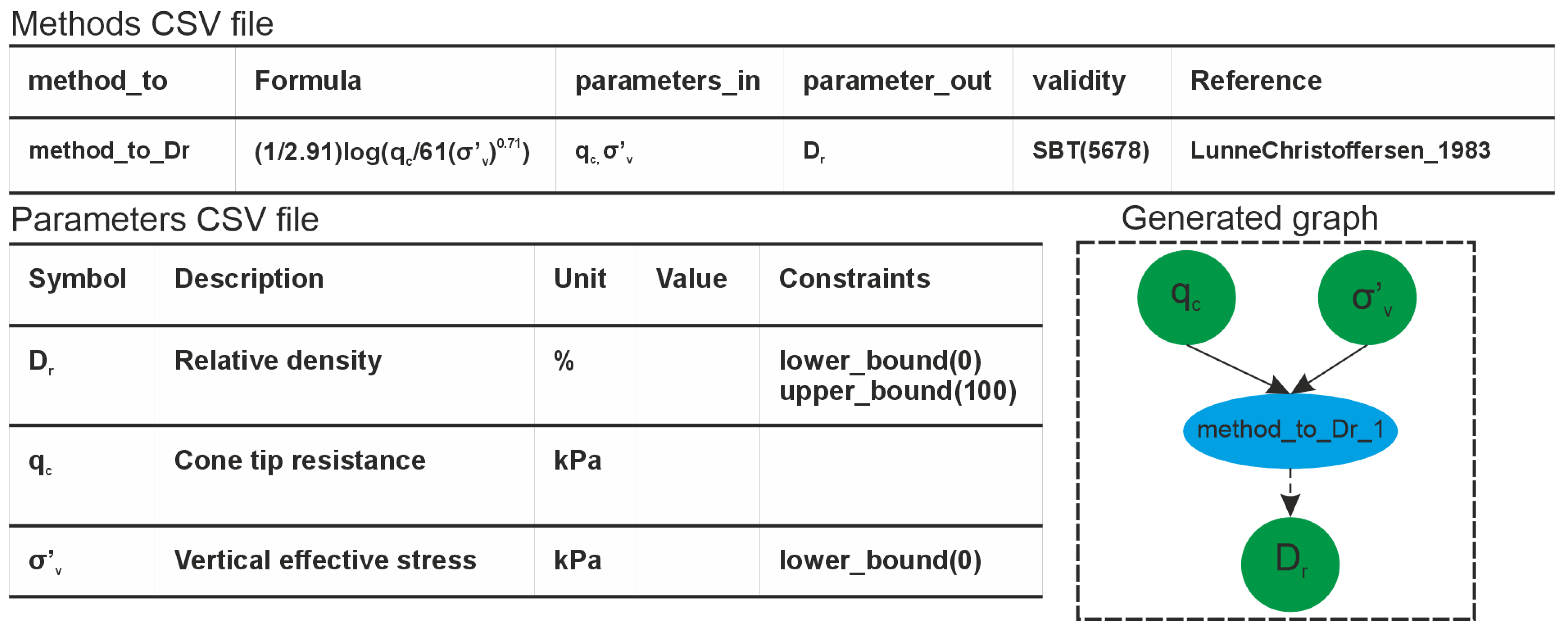
Graphs are generated from two CSV files specifying methods (correlations) and parameters. The system allows filtering by soil type, applicability ranges, and user-defined constraints. An example is shown in Figure 1, where a correlation for the relative density ($D_r$) is implemented.

The generated graph contains two distinct types of nodes: parameter nodes and method nodes. Parameter nodes are listed in the parameters CSV file, whereas method nodes are described in the methods CSV file. The edges—representing connections between nodes—are determined by the parameters_in and parameters_out fields in the methods CSV. The parameters_in field specifies which parameters serve as inputs to a method node (i.e., incoming edges), while the parameters_out field identifies the parameter produced by the method (i.e., the outgoing edge to a parameter node).

Currently, APD supports three primary workflows, enabling parameter assessment based on cone penetration testing (CPT), dilatometer testing (DMT), and shear wave velocity measurements. To accommodate these workflows, the system includes three validated databases of methods and parameters, collectively containing over 200 correlations. Notably, both soil parameters and constitutive model parameters are stored within the same database.

3. Application of APD to a Soft Clay Site

3.1. Test Site

This research focuses on Leda clays—soft and sensitive deposits found in eastern Canada. To facilitate detailed geotechnical investigation, the National Research Council of Canada (NRCC) established the Canadian Geotechnical Research Site No. 1 at South Gloucester, Ontario [7]. Early geotechnical investigations, beginning around 1954, addressed issues such as excessive settlements and poor shallow foundation performance [8]. Several years later, Bozozuk [9] conducted a comprehensive geotechnical study on the site. Other significant studies on the characterisation of this test site include works by [10,11].

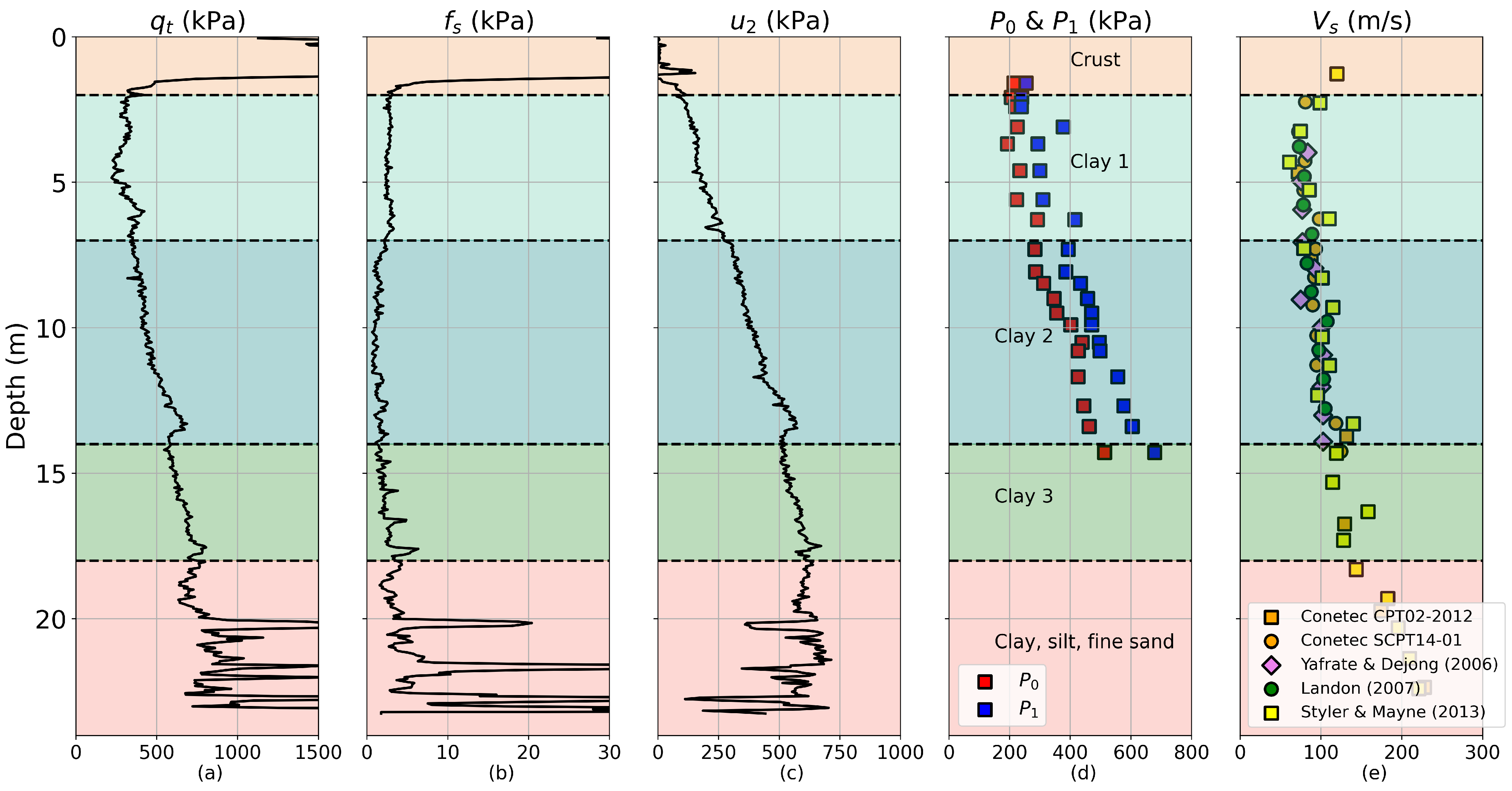
The initial soil stratification identified nine distinct soil layers. Subsequently, a simplified profile was established, which includes a 2-m crust underlain by three soft clay layers extending to a depth of 18 m [7]. Figure 2 presents the results of CPTu sounding (CPT 12-03 from [7]), DMT sounding (extracted from [7]) in the form of the corrected first and second readings ($P_0$ and $P_1$, respectively), and various shear wave velocity ($V_s$) profiles (as reported in [7]). The delineated layers are highlighted in the figure. For the upper crustal layer, the maximum recorded corrected cone resistance ($q_t$) was 6.5 MPa, and the maximum recorded sleeve friction ($f_s$) was 118 kPa. The scales for $q_t$ and $f_s$ in Figure 2a,b have been clipped to improve visibility and facilitate comparison within the soft Leda clay layers. Beneath the crustal layer, $q_t$ generally increases with depth, ranging from 200 to 850 kPa. Similarly, the porewater pressure measurements ($u_2$) increase with depth below the crust, with values ranging between 150 and 650 kPa. The $f_s$ measurements are near the lower limit of strain gauge resolution for CPT sleeve readings in commercial penetrometers, with values typically below 5 kPa [7].

Several research groups have conducted $V_s$ measurements at the site, primarily using the downhole test (DHT) mode via seismic piezocone tests (SCPTu) [12,13]. The overall trend of $V_s$ at the site (Figure 2e) shows a slight decrease in the upper crustal region, reaching a minimum at a depth of approximately 4 m, where $V_s$ values drop as low as 60 m/s. Beyond this depth, $V_s$ steadily increases, reaching 230 m/s at around 22 m. The lowest $V_s$ values at 4 m correspond to a zone with high natural water content [7].

The soft clay layers at Gloucester are slightly overconsolidated, likely due to a combination of aging, secondary compression, minor erosion, and bonding from geochemical processes. The groundwater table is relatively shallow, located approximately 0.8 m below ground level [7].

Figure 2. Results of selected in situ tests, (a–c): CPTu results (profiles of $q_t$, $f_s$ and $u_2$); (d): DMT results ($P_0$ and $P_1$); (e): $V_s$ profiles [11,13,14] (as cited in [7]).

Figure 2. Results of selected in situ tests, (a–c): CPTu results (profiles of $q_t$, $f_s$ and $u_2$); (d): DMT results ($P_0$ and $P_1$); (e): $V_s$ profiles [11,13,14] (as cited in [7]).

3.2. Soil Parameters

In the following sections, the methods selected for determining the unit weight (${\gamma }_t$), overconsolidation ratio ($OCR$), undrained shear strength ($s_u$), and the small-strain shear modulus ($G_0$) from the three workflows of APD (CPT, DMT, and $V_s$) are presented.

3.2.1. Unit Weight

The five modules of APD were briefly introduced in Section 2 and are discussed in detail in [3]. Estimating the unit weight early in module 1 is crucial, as it is required to compute intermediate CPT and DMT parameters that depend on stress inputs. Therefore, an initial unit weight is determined in module 1. This value can be defined using any method or reference value. Selected methods for estimating unit weight across the three workflows are presented in

Table 1. Selected methods for the unit weight (${\gamma }_t$).

Workflow	Method		Author
CPT	${\displaystyle {\gamma }_w[0.27(log{R}_f)+0.36(log{q}_t/p_a)+1.236]}$	(1)	[16]
	${\displaystyle 19.5-2.87\left[\frac{log\left(\frac{9000}{q_t}\right)}{log\left(\frac{20}{R_f}\right)}\right]}$	(2)	[17]
	${\displaystyle 26-\frac{14}{1+{[0.5log{f}_s+1]}^2}}$	(3)	[18]
	${\displaystyle 0.254·log\left(\frac{q_t-u_2}{p_a}\right)+1.54}$	(4)	[19]
DMT	from Marchetti’s chart		[15]
	${\displaystyle {\gamma }_w·1.31{\left(\frac{P_1}{p_a}\right)}^{0.161}}$	(5)	[20]
	${\displaystyle {\gamma }_w·1.35{\left(\frac{P_0}{p_a}\right)}^{0.159}}$	(6)	[20]
	${\displaystyle {\gamma }_w·1.32{\left(\frac{P_1}{p_a}\right)}^{0.091}{\left(\frac{P_0}{p_a}\right)}^{0.0733}}$	(7)	[20]
	${\displaystyle {\gamma }_w·1.47{\left(\frac{E_D}{p_a}\right)}^{0.045}}$	(8)	[20]
$V_s$	${\displaystyle 8.31log{V}_s-1.61logz}$	(9)	[21]
	${\displaystyle 4.17ln{V}_{s1}-4.03}$	(10)	[22]
	${\displaystyle \frac{6.87V_s^{0.227}}{{{\sigma }^{\prime }}_v^{0.057}}}$	(11)	[23]
	${\displaystyle 4.96+5.97log{V}_s}$	(12)	[24]

Note: ${\gamma }_w$ = unit weight of water; $R_f$ = friction ratio; $p_a$ = atmospheric pressure; $E_D$ = dilatometer modulus; z = depth; ${\sigma }_v^{\prime }$ = vertical effective stresses; $V_{s1}$ = effective stress-normalised shear wave velocity ($V_{s1}=V_s/{({\sigma }_v^{\prime }/p_a)}^{0.25}$).

. In this study, the initial unit weight for both the CPT- and $V_s$-based workflows was calculated using Equation (4) (Table 1), while for the DMT-based workflow, it was determined using Marchetti’s chart [15].

3.2.2. Stress History

Stress history is commonly characterised using the overconsolidation ratio (OCR). The selected methods for computing OCR are presented in

Table 2. Selected methods for the overconsolidation ratio ($OCR$).

Workflow	Method		Author
CPT	${\displaystyle \frac{0.33{(q_t-{\sigma }_v)}^{m^{\prime }}}{{\sigma }_v^{\prime }}}$; ${\displaystyle m^{\prime }=1-\frac{0.28}{1+{\left(\frac{I_{cn}}{2.65}\right)}^{25}}}$	(13)	[25,26]
	${\displaystyle 0.25Q_t^{1.25}}$	(14)	[27]
	${\displaystyle 0.2+0.39Q_t}$	(15)	[28]
	${\displaystyle 1.02B_q^{-1.077}}$	(16)	[29]
	${\displaystyle 0.63B_q^{-1.286}}$	(17)	[30]
DMT	${\displaystyle {\left(0.5K_D\right)}^{1.56}}$	(18)	[31]
	${\displaystyle 2{\left(\frac{P_0-{\sigma }_v}{6.63{\sigma }_v^{\prime }}\right)}^{1.19}}$	(19)	[32]
	${\displaystyle 0.24K_D^{1.32}}$	(20)	[33]
	${\displaystyle -0.0135K_D^2+0.4959K_D-0.0359}$	(21)	[34]
$V_s$	${\displaystyle \frac{0.01V_s^2}{{\sigma }_v^{\prime }}}$	(22)	[35]
	${\displaystyle \frac{0.106V_s^{1.47}}{{\sigma }_v^{\prime }}}$	(23)	[36] as cited in [35]
	${\displaystyle \frac{0.007691V_s^{2.009}}{{\sigma }_v^{\prime }}}$	(24)	[37]
	${\displaystyle \frac{0.1097V_s^{1.3575}}{{\sigma }_v^{\prime }}}$	(25)	[24]

Note: I_cn = normalised soil behaviour type (SBT) index; Q_t = normalised cone resistance; B_q = pore pressure parameter ratio; K_D = horizontal stress index.

. It is important to note that some of these methods require effective vertical stresses, which are calculated based on the initial unit weight (discussed in Section 3.2.1).

3.2.3. Strength Parameters

Table 3. Selected methods for the undrained shear strength ($s_u$).

Workflow	Method		Author
CPT	${\displaystyle \frac{q_t-{\sigma }_v}{N_{kt}}}$; ${\displaystyle N_{kt}=12}$	(26)	[38]
	${\displaystyle \frac{q_t-{\sigma }_v}{N_{kt}}}$; ${\displaystyle N_{kt}=10.5-4.6ln(B_q+0.1)}$	(27)	[19]
	${\displaystyle \frac{u_2-u_0}{N_{\Delta u}}}$; ${\displaystyle N_{\Delta u}=6}$	(28)	[38]
	${\displaystyle \frac{u_2-u_0}{N_{\Delta u}}}$; ${\displaystyle N_{\Delta u}=7.9+6.5ln(B_q+0.3)}$	(29)	[19]
	${\displaystyle \frac{q_t-u_2}{N_{ke}}}$; ${\displaystyle N_{ke}=8}$	(30)	[38]
	${\displaystyle \frac{q_t-u_2}{N_{ke}}}$; ${\displaystyle N_{ke}=4.5-10.66ln(B_q+0.2)}$	(31)	[19]
DMT	${\displaystyle 0.12(P_0-{\sigma }_v)}$	(32)	[32]
	${\displaystyle 0.09(P_1-{\sigma }_v)}$	(33)	[32]
	${\displaystyle 0.22{\sigma }_v^{\prime }{\left(0.5K_D\right)}^{1.25}}$	(34)	[31]
	${\displaystyle 0.018\left(E_D\right)}$	(35)	[39]
	${\displaystyle 0.35{\sigma }_v^{\prime }{\left(0.47K_D\right)}^{1.14}}$	(36)	[39]
$V_s$	${\displaystyle 0.152V_s^{1.142}}$	(37)	[40]
	${\displaystyle 0.021V_s^{1.52}}$	(38)	[37]
	${\displaystyle 0.016V_s^{1.50}}$	(39)	[24]

presents the selected methods for determining undrained shear strength ($s_u$). The bearing factors for net tip resistance, excess porewater pressure, and effective cone resistance are denoted as $N_{kt}$ (Equations (26) and (27)), $N_{\Delta u}$ (Equations (28) and (29)), and $N_{ke}$ (Equations (30) and (31)), respectively. Recommended average values are 12 for $N_{kt}$ (Equation (26)), 6 for $N_{\Delta u}$ (Equation (28)), and 8 for $N_{ke}$ (Equation (30)) [38]. Several studies have shown that $N_{kt}$ and $N_{ke}$ vary inversely with $B_q$ (Equations (27) and (31)), while $N_{\Delta u}$ varies directly with $B_q$ (Equation (29)) [19].

3.2.4. Stiffness Parameters

The small-strain shear modulus ($G_0$) is determined from $V_s$ using Equation (52), where $\rho$ represents the soil density. For the CPT-based workflow, $G_0$ is computed using Equation (52), with $V_s$ values derived from the methods listed in

Table 4. Selected methods for the shear wave velocity ($V_s$).

Workflow	Method		Author
CPT	${\displaystyle {(10.1log{q}_c-11.4)}^{1.67}{(f_s/q_c\times 100)}^{0.3}}$	(40)	[41]
	${\displaystyle 3.18q_c^{0.549}{f}_s^{0.025}}$	(41)	[41]
	${\displaystyle {[{\alpha }_{vs}(q_t-{\sigma }_v)/p_a]}^{0.5}}$; ${\displaystyle {\alpha }_{vs}={10}^{(0.55I_{cn}+1.68)}}$	(42)	[42]
	${\displaystyle 1.75q_c^{0.627}}$	(43)	[43]
	${\displaystyle 6.53{(q_c-{\sigma }_v)}^{0.461}}$	(44)	[43]
	${\displaystyle 2.944q_t^{0.613}}$	(45)	[44]
	${\displaystyle 14.4{(q_t-{\sigma }_v)}^{0.265}{\left({\sigma }_v^{\prime }\right)}^{0.137}}$	(46)	[45]
	${\displaystyle 7.95q_t^{0.403}}$	(47)	[46]
	${\displaystyle 4.541q_t^{0.487}{(1+B_q)}^{0.337}}$	(48)	[46]
	${\displaystyle 8.35{(q_t-{\sigma }_v)}^{0.22}{\left({\sigma }_v^{\prime }\right)}^{0.357}}$	(49)	[37]

. The selected methods for calculating $G_0$ are presented in

Table 5. Selected methods for the small-strain shear modulus ($G_0$).

Workflow	Method		Author
DMT	${\displaystyle 7.5E_D}$	(50)	as mentioned in [47]
	${\displaystyle 26.177K_D^{-1.0066}{M}_{DMT}}$; for $I_D<0.6$	(51)	[48]
$V_s$	${\displaystyle \rho V_s^2}$	(52)

Note: $M_{DMT}=R_M{E}_D$, for $I_D<0.6$, $R_M=0.14+2.36log{K}_D$ [31,49].

.

3.3. Results

Section 3.2.1, Section 3.2.2, Section 3.2.3 and Section 3.2.4 detail the selected methods for deriving soil parameters from CPTu, DMT, and $V_s$ profiles, as shown in Figure 2. In this study, the $V_s$ profiles (Figure 2e) were consolidated into a single representative profile. APD computes parameters based on predefined layers, which are determined in module 2 (see Section 2). The stratification process, including the algorithms and approaches, is discussed in Section 5.1.

For the determination of soil parameters and their comparison with reference values interpreted at the test site, manual stratification was employed. CPTu and $V_s$ data were averaged at 1 m intervals for input into the analysis. Given the lower measurement frequency of DMT, smaller averaging intervals (0.4–0.8 m) were applied. This manual layering and averaging process ensured an appropriate number of layers for meaningful comparisons between in situ test data and reference values. Since APD computes parameters based on layers, selecting thinner layers (e.g., 1 m for the CPT-based workflow) increases the total number of layers and, consequently, the number of generated graphs.

Since the layers are manually defined, the user must assign an SBT to each layer, which serves as a validity criterion for the methods CSV file. In this study, the test site consists of a sensitive clay deposit. Therefore, all layers beneath the crust were assigned SBT(1-3), as per [50]. The averaging process resulted in 23 layers for the CPTu and $V_s$ profiles and 18 layers for the DMT. It is important to note that the $V_s$ profiles were incorporated as an add-on to the CPT-based workflow.

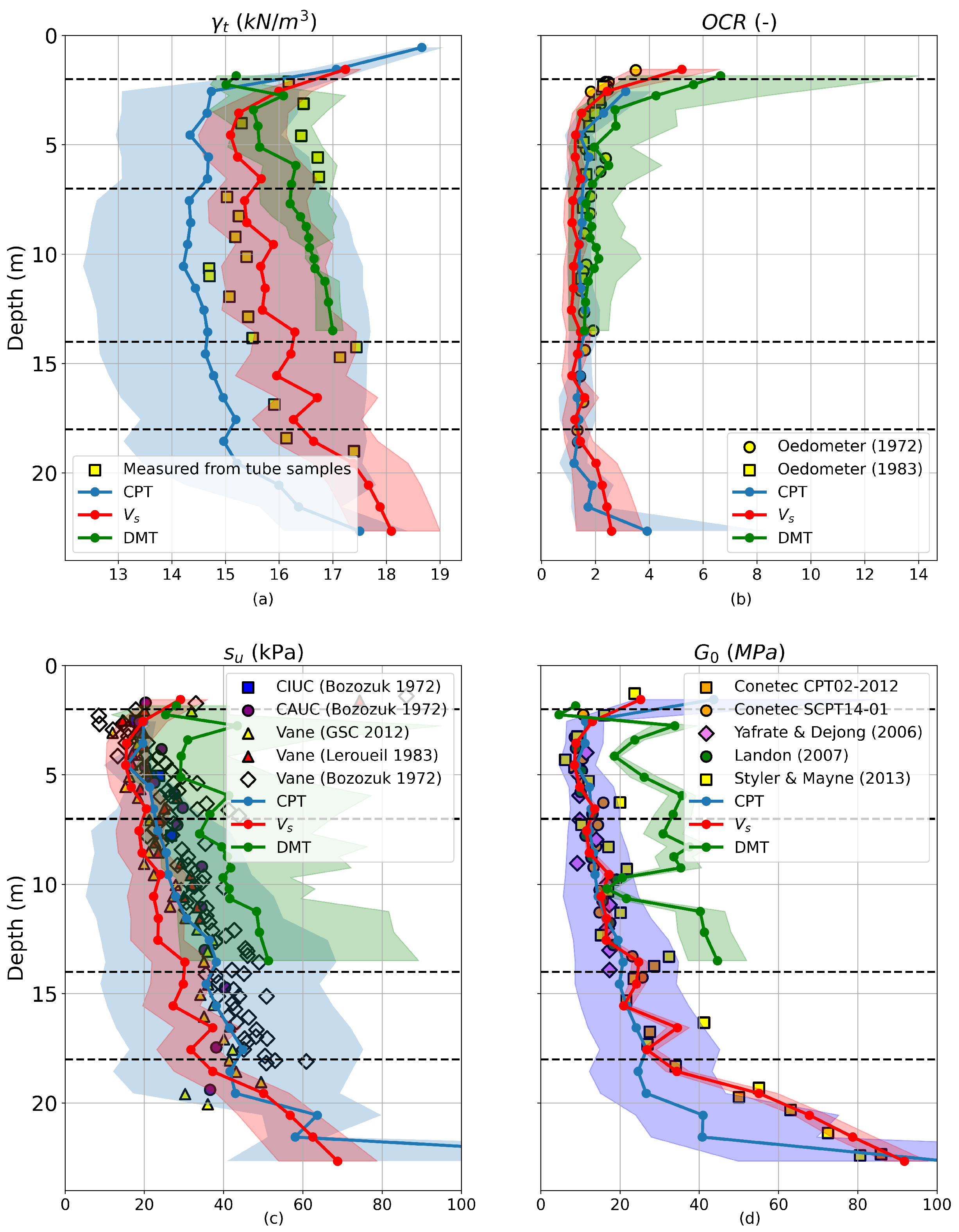
Figure 3 illustrates the comparison between APD results—generated using the methods outlined in the previous subsections—and the benchmark values interpreted at the Leda clay site. The highlighted regions in blue, green, and red correspond to the value ranges obtained from the CPT, DMT, and shear wave velocity ($V_s$) workflows, respectively. Solid lines with circular markers in matching colors indicate the mean values for each workflow. These markers are positioned at the mid-depths of the respective thin layers.

The total unit weight was determined from tube sampling, as reported in [7]. Figure 3a displays the outcomes of the three workflows based on the methods summarised in Table 1. For the CPT-based workflow, the upper limit of the predicted range (blue highlighted area) shows good agreement with the reference data in Clay 1 and Clay 3 (see Figure 2), suggesting that certain methods provided reliable estimates. Nevertheless, the majority of CPT-based methods yielded lower values than those measured, which can be attributed to the low $f_s$ values and ultimately led to an underestimation in the average CPT-derived results. In contrast, the average values from the $V_s$-based workflow show good agreement with the reference values. For the DMT-based workflow, the predicted unit weight aligns well with the reference values in Clay 1 but is overestimated in Clay 2.

The evaluation of OCR was based on oedometer tests [9,10], as cited in [7]. Figure 3b presents the OCR values obtained using the methods listed in Table 2. The average predictions from the three workflows align closely with the reference OCR values, demonstrating good overall agreement.

The “reference” $s_u$ values were collected from various sources, as cited in [7], with these sources highlighted in the legend of Figure 3c. The average predictions from the CPT-based workflow provided reasonable estimates of the reference values. Notably, the cone factors that depend on $B_q$ (Equations (27), (29) and (31)) performed significantly better than the fixed cone factors (Equations (26), (28) and (30)). The predictions from the DMT-based workflow tend to overestimate the reference $s_u$ values (as shown by the upper green bound). The average predictions from the $V_s$-based workflow correspond closely to the lower end of the reference values.

Reference $G_0$ values were derived from the $V_s$ profiles presented in Figure 2e using Equation (52). A constant total density of 1.65 $t/m^3$ was used to convert the $V_s$ profiles to $G_0$, as reported in [11]. Table 5 presents the methods selected for computing $G_0$, and Figure 3d shows the results. Starting with the $V_s$-based workflow, unit weights computed from Equations (9)–(12) were used in Equation (52) to calculate $G_0$. It is clear that the $V_s$-based workflow produces the most reliable $G_0$ values, as it directly uses measured $V_s$ as input. The predictions from the DMT-based workflow tend to significantly overestimate the in situ $G_0$ values, whereas the average predictions from the CPT-based workflow provide a reasonable fit for the layers of Clay 1, 2, and 3.

4. Application of APD to Other Sites

To illustrate the generalisability and adaptability of the Automated Parameter Determination (APD) system, this section showcases its application at three Norwegian GeoTest Sites (NGTS), each representing a different soil type: clay, silt, and sand. These case studies underscore APD’s capability to process site investigation data across varied geological conditions. The analyses demonstrate the system’s reliability in addressing diverse ground conditions and its usefulness in early-stage design and site assessment tasks. In all three cases, the required in situ test data were obtained via the online platform Datamap [51]. The findings reinforce APD’s effectiveness in deriving soil parameters directly from field-based measurements.

4.1. Onsøy Soft Clay Site

The NGTS soft clay site at Onsøy, established in 2016, has been the focus of an extensive laboratory and field testing program. In situ tests included piezocone tests (CPTu), seismic cone penetration tests (SCPT), seismic flat dilatometer tests (SDMT), and self-boring pressuremeter tests (SBPMT). Laboratory investigations involved determining in situ water content, unit weight, and Atterberg limits, as well as conducting constant rate of strain oedometer (CRS) tests, triaxial tests, and direct simple shear (DSS) tests. Both block and various types of tube samplers were used for sample recovery [52].

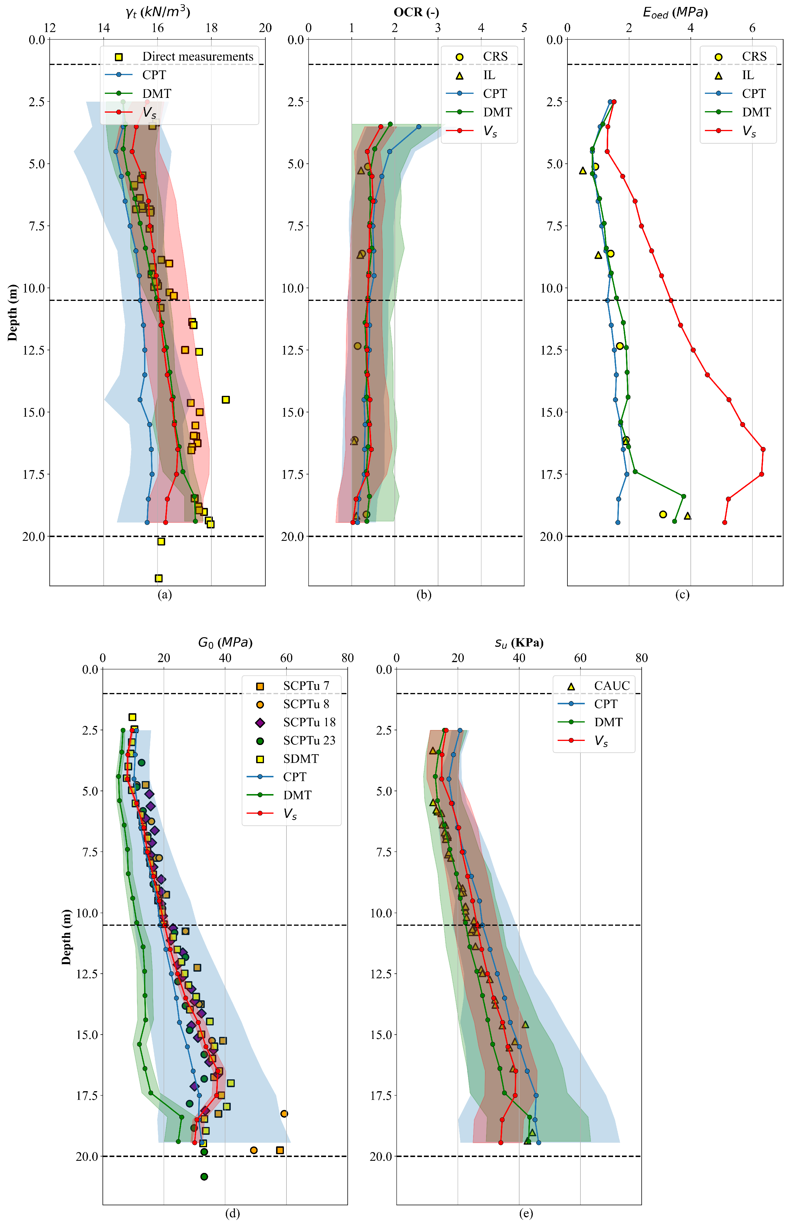
The in situ tests selected as input for APD, along with the corresponding methods and additional details about the Onsøy soft clay site, are presented in [3]. A comparison between the APD-generated results and the reference values interpreted for this site is shown in Figure 4.

Figure 4a presents the estimated total unit weight. The output of the CPT-based workflow shows that certain methods—particularly those reflected by the upper limit of the blue-shaded area—closely match the reference data. Nonetheless, as most CPT methods tend to yield lower values, the overall CPT average also underestimates the measured unit weight. In contrast, the DMT- and $V_s$-based approaches produce average values that closely align with the reference measurements. Figure 4b shows the overconsolidation ratio (OCR) estimates. The mean results from all three methods indicate a slightly overconsolidated condition, consistent with the reference interpretation.

Figure 4c indicates that the CPT-based workflow provides estimates of $E_{oed}$ that are generally consistent with the reference values, except in the final layer where it underestimates stiffness. The DMT-based workflow also yields reliable $E_{oed}$ estimates, while the $V_s$-based workflow tends to overestimate the reference values. Regarding the small-strain shear modulus $G_0$ (Figure 4d), the $V_s$-based workflow results in the most reliable predictions, which is expected since it directly utilises measured $V_s$ data. In contrast, the DMT-based workflow significantly underestimates $G_0$, and the CPT-based workflow provides a wide range of values. Nonetheless, in this case study, the average of the CPT-based range aligns well with the reference values. For undrained shear strength $s_u$ (Figure 4e), the DMT-based workflow shows overall good agreement with the reference values. The $V_s$-based workflow overestimates $s_u$ in the upper layer but provides reasonable predictions in the lower layer. On average, the CPT-based workflow tends to overestimate the reference $s_u$ values.

4.2. Halden Silt Site

The Halden site is located in Southeastern Norway, approximately 120 km south of Oslo, and covers an area of about 6000 m² with predominantly flat topography. It has been extensively characterised through a combination of geological, geophysical, and geotechnical investigation techniques [53].

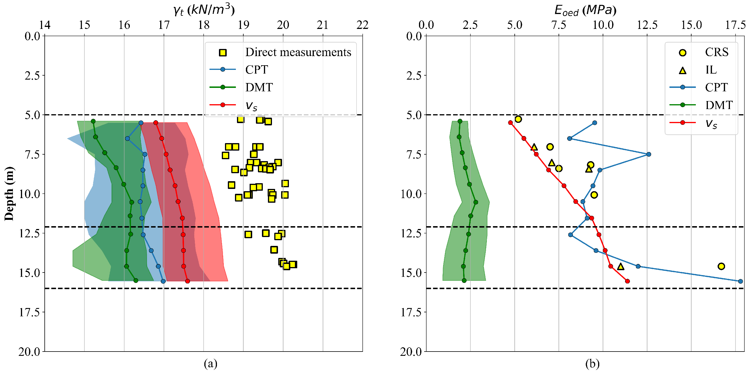
The in situ tests selected as input for APD, along with the associated methods and further details about the Halden silt site, are provided in [6]. A comparison between the results generated by APD and the reference values interpreted for this site is presented in Figure 5.

Performing DMT in silty soils can lead to partial drainage during membrane expansion, potentially affecting the DMT readings and introducing errors when deriving parameters using standard DMT correlations [54]. Correction methods, such as the approach proposed by [55], can be employed to account for these effects. However, for the DMT tests conducted at this site, correction for partial drainage was not possible due to the lack of time-dependent data.

Figure 5a presents the measured unit weights alongside the values estimated by the three workflows. None of the selected methods succeeded in accurately predicting the measured unit weight, although the methods employed in the $V_s$-based workflow yielded the highest ${\gamma }_t$ values. Alternative approaches for improving the prediction of ${\gamma }_t$ include the use of machine learning techniques, such as the study presented in [56]. A crucial factor in the successful application of machine learning models is the quality and representativeness of the training databases. In the aforementioned study, an open-access CPT database was utilised for model training [57].

Figure 5b shows that both the CPT- and $V_s$-based workflows yield good to reasonable estimates for $E_{oed}$. In contrast, the DMT-based workflow underestimates the reference values in this case, likely due to partial drainage effects. One consequence of partial drainage is that the difference between the two DMT readings becomes too small, resulting in low values of $I_D$ and, consequently, underestimated $E_{oed}$ values [54].

As illustrated in Figure 5c, the $V_s$-based workflow delivers the most accurate estimation of the small-strain shear modulus, $G_0$. Overall, the CPT-based workflow estimates of $G_0$ typically fall below the in situ reference values, and a similar underestimation trend is observed for most methods within the DMT-based workflow. With regards to the undrained shear strength, $s_u$ (Figure 5d), the CPT-based workflow demonstrates a reasonable agreement with the values interpreted from anisotropically consolidated undrained triaxial (CAUC) tests. The $s_u$ estimates from the $V_s$-based approach generally lie between the reference results from CAUC and direct simple shear (DSS) tests, while the values obtained from the DMT-based worfklow tend to underestimate $s_u$ compared to the reference data.

4.3. Øysand Site

The Øysand test site is located approximately 15 km southwest of Trondheim, Norway. Site characterisation at the Øysand research facility began in 2016 as part of the NGTS project. Since then, a wide range of in situ tests, geophysical surveys, sampling techniques, and laboratory investigations have been conducted to assess the geological history and geotechnical properties of the sand deposits [58].

The CPT results used as input for APD, along with the associated methods and additional details about the Øysand site, are provided in [59]. A comparison between the results generated by APD and the reference values interpreted for this site is shown in Figure 6. The results are presented for the sand layer (between 12 and 18 m).

The total unit weight was indirectly determined from water content measurements of the samples, assuming full saturation [58]. However, the water content measurements from disturbed samples were found to be lower than expected, likely due to sample disturbance [60]. Water migration during sampling, transportation, and storage can lead to such discrepancies [60]. As a result, the actual in situ unit weight is expected to be lower than the reported values. The results obtained from the CPT-based workflow are shown in Figure 6a. Overall, the methods tend to underestimate the reported values; however, considering that these reference values are based on disturbed samples, lower in situ values are anticipated.

Five isotropically consolidated triaxial tests—three undrained (IUC) and two drained (IDC)—were performed on undisturbed (frozen) samples collected at depths of 13.3, 13.8, 14.1, 14.3, and 14.6 m [60]. Accordingly, five reference values are reported for $e_0$, $D_r$, and ${\phi }_p^{\prime }$, as highlighted in Figure 6b–d. Figure 6b presents the values obtained from the CPT-based workflow, using the unit weights shown in Figure 6a as input.

The reference relative density values are significantly influenced by the method used to determine $e_{min}$ and $e_{max}$ in the laboratory [60]. The values obtained from the CPT-based workflow are presented in Figure 6c. As shown in the figure, the upper bound of the range successfully captures the first three reference values, while the lower bound captures the two lower reference values. On average, the CPT-based methods underestimate the first three reference values and overestimate the last two. The peak friction angles were determined from three undrained isotropically consolidated (IUC) and two drained isotropically consolidated (IDC) triaxial tests, as highlighted in Figure 6d. With the exception of the fourth reference value (at a depth of 14.3 m), the methods predict the peak friction angles reasonably well. The reference values for the shear wave velocity were derived from the seismic SCPT20 (OYSC20 in the project) test. As shown in Figure 6e, the CPT-based workflow provides a reasonable prediction of the in situ $V_s$ values.

5. Connection to Numerical Modelling

The primary aim of the APD system is to produce material datasets suitable for direct use in numerical analysis. This process depends on two fundamental components: the stratigraphic profile and the parameters required for constitutive modelling. Stratigraphy is defined within module 2, whereas the constitutive parameters are derived using methods selected by the user. There are no inherent restrictions on the choice of constitutive model; users are free to adopt any model, provided that the required parameters can be obtained. Generally, the workflow involves first determining relevant soil properties, after which an appropriate constitutive model is selected based on the soil type. The corresponding model parameters are then derived from the previously determined soil properties.

5.1. Stratification

Several stratification methods implemented in APD are based on soil behaviour type (SBT) charts, which are determined using one of three commonly used charts: Robertson’s normalised SBT chart [27], modified non-normalised SBT chart [50], or the updated normalised SBT chart [61].

For each CPT measurement, the SBT is assigned using one of these classification charts. APD currently supports three distinct approaches to generating soil layers from CPT profiles. The first two are automated techniques that cluster consecutive CPT readings sharing the same SBT classification. Layer interfaces are introduced at locations where a notable shift in SBT occurs, resulting in a segmented CPT profile composed of a limited number of layers, each characterised by its average SBT. The third method is a manual approach (applied in the case study presented in Section 3.3), where the user defines the stratigraphic boundaries, and these inputs are preserved throughout the stratification process.

Additionally, other automated stratification approaches from the literature (e.g., [62]) can be applied. Methods employing machine learning (ML) models, such as those proposed in [63], can also be incorporated into the APD framework. External tools, like the CPT interpretation software package CPeT-IT v3.0 [64], can also be utilised for stratification purposes. In general, any suitable method can be integrated into the automated system, which makes the system again very adaptable.

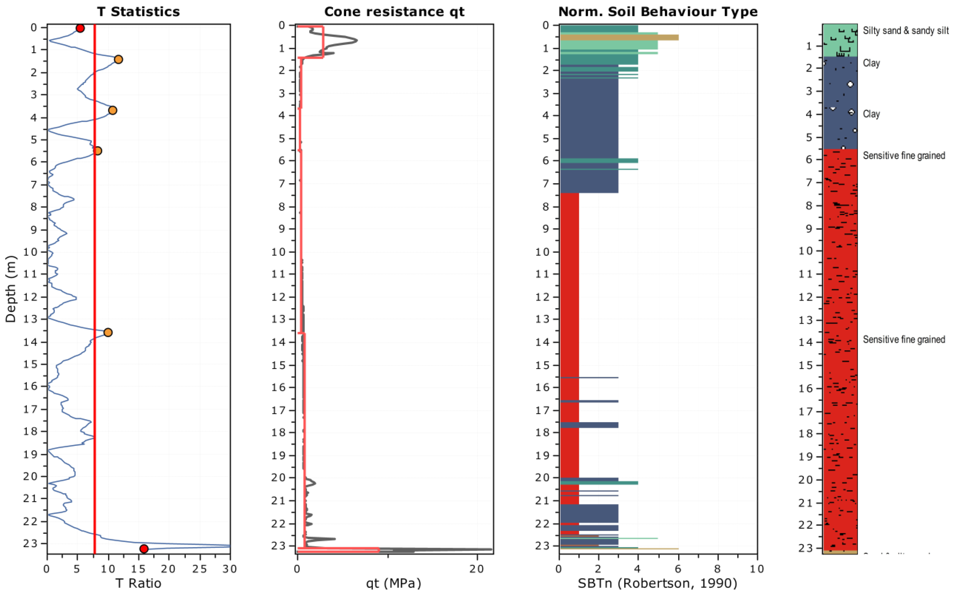
In the following study, CPeT-IT (version 3.9.5.9) was used as the source for stratification. The CPTu sounding, presented in Figure 2a–c, was imported and stratified using CPeT-IT. The layer detection algorithm implemented in CPeT-IT follows the method outlined by [65], based on a simple univariate statistical analysis of the $q_t$, normalised cone resistance corrected for stress level ($Q_{tn}$), $I_{cn}$, or modified soil behaviour type index ($I_B$) profiles. For this study, the analysis was performed using the $I_{cn}$ profile. The resulting stratification is shown in Figure 7. The algorithm detects soil layer boundaries based on the peaks in the T Ratio plot (Figure 7). The vertical red line in the T Ratio plot represents the threshold value for identifying significant peaks. A minimum layer thickness of 0.5 m and a window width of 30 points were set. The T Ratio plot is then generated based on the selected window width, with high values indicating significant changes in the parameter, suggesting a transition between soil layers. This approach resulted in six distinct layers, with the upper crust (top 1.45 m) identified as silty sand and sandy silt. Below this, two clay layers were detected, followed by two sensitive fine-grained layers, and a very thin sand and silty sand layer at the end of the sounding. Comparing the obtained stratification with the interpreted profile at the test site (Figure 2), the upper crust layer was accurately identified. The subsequent fine-grained layers also align well with the interpreted soil profile, whether considering the initial stratification with nine soil layers or the simplified version with three soft clay layers.

5.2. Constitutive Model Parameters

In this section, the constitutive model parameters for the layers identified in Section 5.1 are determined. The very thin sand and silty sand layer detected at the end of the sounding is excluded from the numerical modelling. Consequently, parameters are determined only for the first five layers.

Stress dependency of stiffness plays a crucial role in the numerical modelling of various geotechnical problems, especially when dealing with settlement prediction [66]. This aspect is incorporated in the Hardening Soil (HS) model [67], which accounts for both shear and compression hardening by implementing a cone and a cap yield surface. Additionally, the non-linear degradation of shear stiffness with shear strain can be captured using an extension of the HS model, namely the Hardening Soil model with small-strain stiffness (HSsmall) [68].

5.2.1. Layer 1

Layer 1 is modelled using the HS model as a drained material. The peak friction angle (${\phi }_p^{\prime }$) is determined from the CPT-based workflow, taking the average of the three methods presented in Table 6. The stiffness parameters for the HS model are derived from the $V_s$-based workflow. The range between the constrained modulus ($E_{oed}$) and $G_0$ spans from 0.02 for organic plastic clay to 2 for overconsolidated quartz sands [69]. For this sandy silt layer, an $E_{oed}/G_0$ ratio of 0.3 was selected. The reference stiffness parameters for the HS model are calculated as follows:

$$E_{oed}=E_{oed}^{ref}{\left[{\displaystyle \frac{c^{\prime }cos{\phi }^{\prime }+{\sigma }_1^{\prime }sin{\phi }^{\prime }}{c^{\prime }cos{\phi }^{\prime }+p^{ref}sin{\phi }^{\prime }}}\right]}^m$$

(53)

$$E_{50}=E_{50}^{ref}{\left[{\displaystyle \frac{c^{\prime }cos{\phi }^{\prime }+{\sigma }_3^{\prime }sin{\phi }^{\prime }}{c^{\prime }cos{\phi }^{\prime }+p^{ref}sin{\phi }^{\prime }}}\right]}^m$$

(54)

$$E_{ur}=E_{ur}^{ref}{\left[{\displaystyle \frac{c^{\prime }cos{\phi }^{\prime }+{\sigma }_3^{\prime }sin{\phi }^{\prime }}{c^{\prime }cos{\phi }^{\prime }+p^{ref}sin{\phi }^{\prime }}}\right]}^m$$

(55)

where $c^{\prime }$ corresponds to the effective cohesion, ${\sigma }_1^{\prime }$ and ${\sigma }_3^{\prime }$ represent the major and minor principal effective stresses, respectively; $p^{ref}$ is the reference pressure (taken as 100 kPa in this study), and m denotes the stress-dependency exponent.

In this study, $c^{\prime }$ was set to 0 for all soil layers. The relation between different stiffness parameters for layer 1 is defined as follows [70]: $E_{oed}^{ref}=E_{50}^{ref}$ and $E_{ur}^{ref}=4\times E_{50}^{ref}$.

Table 6. Methods for the peak friction angle (${\phi }_p^{\prime }$).

Method		Author
${\displaystyle 17.6+11log\left(Q_{tn}\right)}$	(56)	[71]
${\displaystyle 25{\left(Q_{tn}\right)}^{0.10}}$	(57)	[72] as cited in [73]
${\displaystyle 53-6.9I_{cn}}$	(58)	[19]

Table 6. Methods for the peak friction angle (${\phi }_p^{\prime }$).

Method		Author
${\displaystyle 17.6+11log\left(Q_{tn}\right)}$	(56)	[71]
${\displaystyle 25{\left(Q_{tn}\right)}^{0.10}}$	(57)	[72] as cited in [73]
${\displaystyle 53-6.9I_{cn}}$	(58)	[19]

5.2.2. Layers 2, 3, 4, and 5

Layers 2, 3, 4, and 5 are modelled using the HSS model as undrained materials. For these layers, $E_{oed}$ is determined as the average value from both the CPT- and $V_s$-based workflows, following Equations (59) and (60), as proposed by [42] and [37], respectively.

$$E_{oed}={\alpha }_M(q_t-{\sigma }_v);{\alpha }_M=Q_{tn};for{I}_{cn}\ge 2.2\&Q_{tn}<14$$

(59)

$$E_{oed}=0.00010V_s^{2.212}\times 1000$$

(60)

The relationships between the different stiffness parameters for layers 2, 3, 4, and 5 are defined as follows [70]: $E_{50}^{ref}=1.25\times E_{oed}^{ref}$ and $E_{ur}^{ref}=5\times E_{50}^{ref}$.

The small-strain shear modulus, $G_0$, is obtained from the $V_s$-based workflow, while the reference stiffness parameters for the HSS model were previously defined in Equations (53)–(55). The reference value of $G_0$ ($G_0^{ref}$) is determined as follows:

$$G_0=G_0^{ref}{\left[{\displaystyle \frac{c^{\prime }cos{\phi }^{\prime }+{\sigma }_3^{\prime }sin{\phi }^{\prime }}{c^{\prime }cos{\phi }^{\prime }+p^{ref}sin{\phi }^{\prime }}}\right]}^m$$

(61)

In the HSS model, the small-strain stiffness behaviour is governed not only by $G_0^{ref}$ but also by the threshold shear strain (${\gamma }_{0.7}$), at which the secant shear modulus reduces to 0.722 $G_0$. The value of ${\gamma }_{0.7}$ is determined based on the plasticity index ($PI$) and the overconsolidation ratio ($OCR$) using the following relationship [74]:

$${\gamma }_{0.7}=0.0001+5\times {10}^{-6}PI{\left(OCR\right)}^{0.3}$$

(62)

The plasticity index can be calculated from the CPT measurements using the method described by [75]:

$$PI={\displaystyle \frac{17.5R_f{(1+B_q)}^{1.2}}{{\left(0.33Q_t\right)}^{0.31}}}$$

(63)

OCR is determined as the average value from both the CPT- and $V_s$-based workflows, following the methods defined in Table 2. The coefficient of earth pressure at rest ($K_0$) is determined using the method by [76] as cited in [71]:

$$K_0=(1-sin{\phi }_{cv}^{\prime })OC{R}^{sin {\phi }_{cv}^{\prime }}$$

(64)

where ${\phi }_{cv}^{\prime }$ represents the critical state friction angle. For layers 2 and 3 (clay layers), an average value of 28.6° was adopted, as proposed by [77]. A higher value of 32° was selected for layer 1 (sandy silt), while a lower value of 25° was used for layers 4 and 5 (sensitive fine-grained soils).

The material sets for the five layers are presented in

Table 7. Material sets for the 5 layers.

	Layer 1	Layer 2	Layer 3	Layer 4	Layer 5
Model	HS	HSS	HSS	HSS	HSS
$SB{T}_n$	Silty sand and sandy silt	Clay	Clay	Sensitive fine grained	Sensitive fine grained
Drainage	Drained	Undrained B	Undrained B	Undrained B	Undrained B
${\gamma }_t$ (kN/m3 )	18.83	15.91	14.96	14.59	15.47
$E_{50}^{ref}$ (kPa)	34,400	7761	3461	3780	5638
$E_{oed}^{ref}$ (kPa)	34,400	6209	2769	3024	4511
$E_{ur}^{ref}$ (kPa)	137,600	38,810	17,300	18,900	28,190
${\nu }_{ur}$ (-)	0.2	0.2	0.2	0.2	0.2
m (-)	0.7	1	1	1	1
$G_0^{ref}$ (kPa)	-	47,620	37,260	34,700	54,300
${\gamma }_{0.7}$ (-)	-	$2.09\times {10}^{-4}$	$2.55\times {10}^{-4}$	$1.74\times {10}^{-4}$	$2.10\times {10}^{-4}$
${\phi }^{\prime }$ (°)	37.77	-	-	-	-
$s_u$ (kPa)	-	20.32	16.42	25.85	46.92
$K_0$ (-)	0.8414	0.8601	0.6189	0.6383	0.6834
OCR (-)	3	2.951	1.453	1.306	1.539

. Poisson’s ratio (${\nu }_{ur}$) was set to 0.2 for all layers, while m was assigned a value of 0.7 for layer 1 and 1.0 for the remaining layers. OCR methods often yield unrealistically high values for shallow layers due to very low effective stresses. As a result, the predicted OCR value for layer 1 was deemed unrealistic. Therefore, the OCR value was manually assigned as 3, slightly higher than the value obtained for layer 2. The connection between the determined material sets and a finite element software is discussed in the following section through a simple synthetic case study.

6. Case Study

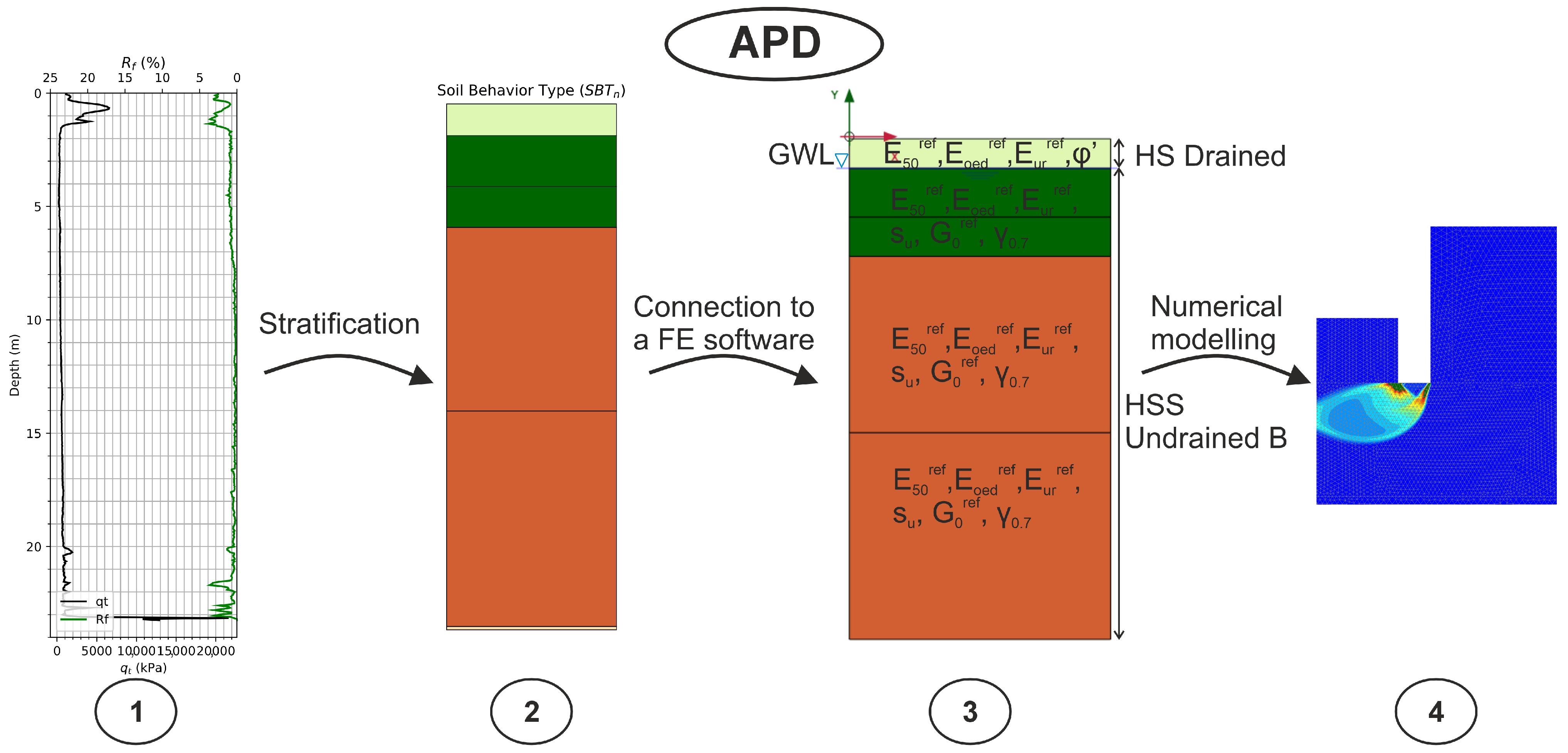
Section 5 outlined the CPT stratification and the determination of constitutive model parameters for different layers. This section demonstrates the full potential of APD through a synthetic case study. The APD workflow is illustrated in Figure 8, beginning with in situ raw measurements. These measurements are first imported into APD, followed by stratification (module 2). Subsequently, soil and constitutive model parameters are evaluated using the graph-based approach (modules 4 and 5). An automatic connection to PLAXIS (version 24.2) [78] is then established, where a borehole is created with the corresponding values, and the constitutive model parameters for each layer are automatically assigned, enabling the user to proceed with the numerical analysis. On a 3.70 GHz CPU, the entire process—from raw data input to borehole definition in PLAXIS—takes approximately 5 s.

Currently, APD processes one CPT at a time. Ongoing research aims to extend the system to handle multiple CPTs simultaneously. This enhancement will enable the generation of more complex subsurface models with inclined or spatially varying layers when transferred to the finite element software.

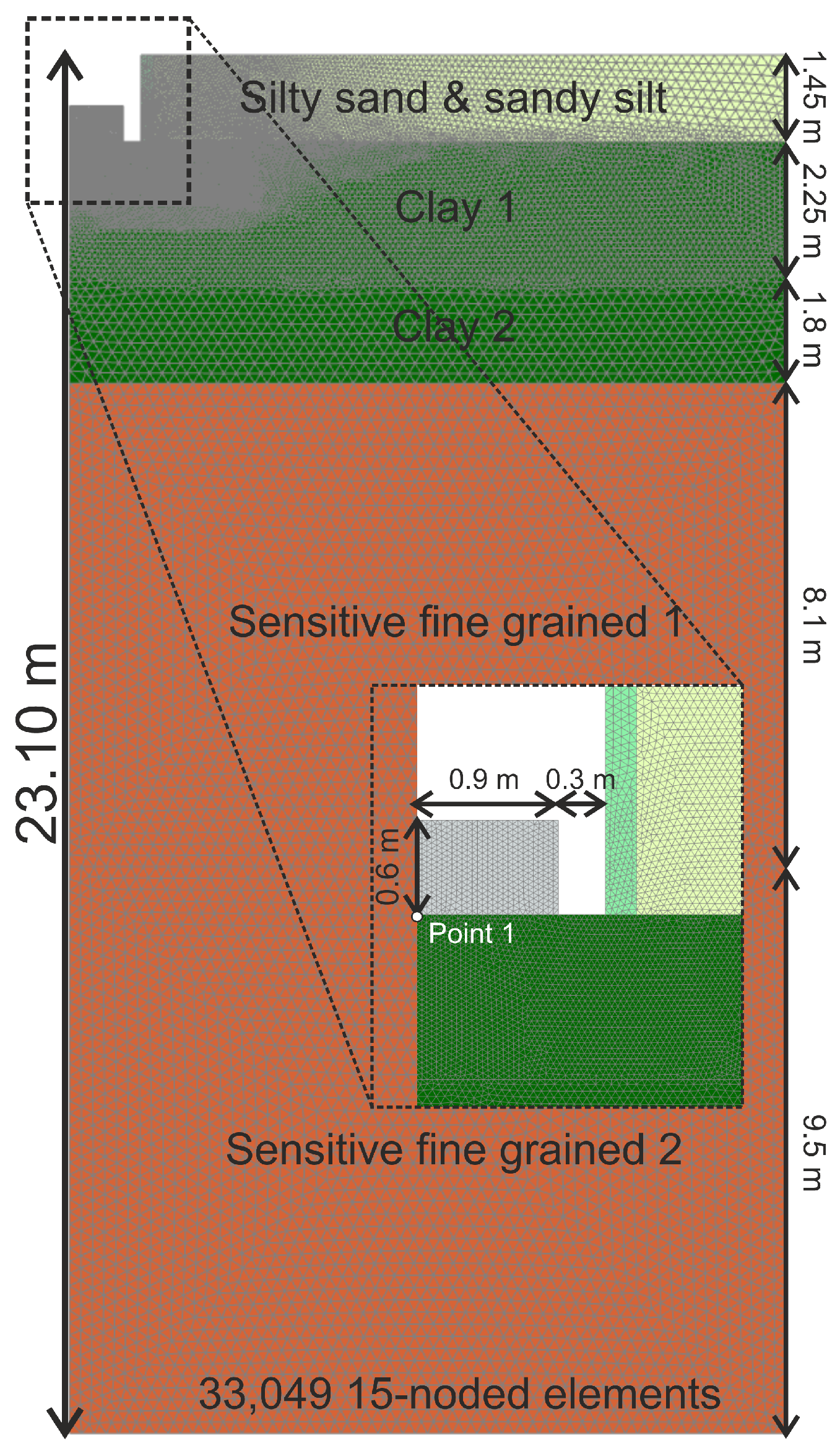
To illustrate the stages outlined in Figure 8, a synthetic case study involving a shallow foundation is modelled. The finite element (FE) axisymmetric model is shown in Figure 9, where a circular footing with a radius of 0.9 m is placed on layer 2 (Clay 1). The footing has a height of 0.6 m, with a 0.3 m gap between the footing and layer 1. The groundwater table is positioned 1.45 m below the ground surface.

The FE model consists of 33,049 15-noded elements, extending to a depth of 23.10 m and a width of 12 m. Point 1 used for plotting the results, is located directly beneath the footing, as highlighted in the figure. The calculation sequence followed these steps:

• Initial stress generation
• Excavation
• Foundation installation
• Loading

The footing was modelled as a linear elastic material representing concrete, with a unit weight of $\gamma =24$ kN/m³. To ensure the stability of layer 1 during excavation, a thin cluster (20 cm wide) was introduced on the left side of the layer. This cluster was assigned the same properties as layer 1, with an additional cohesion of 6 kPa.

The failure mechanism predicted by the finite element analysis (FEA), along with the load-settlement behaviour at Point 1, is presented in Figure 10. The failure load was determined to be 118 kN/m/m.

Using APD in combination with parametrised finite element models enables an almost fully automated process for parameter identification, model generation, and calculation phase definition. By streamlining the transition from in situ test data to numerical modelling, APD reduces manual input and potential errors while ensuring consistency in parameter selection.

This study demonstrates the potential of APD by illustrating its integration into a finite element software. However, the objective of this section is not to identify the optimal constitutive model for this specific soil type or to validate the material parameters through back-analysis of a boundary value problem (BVP). Instead, the focus is on determining the parameters for the HS and HSS models using the CPT- and $V_s$-based workflows to highlight the capabilities of APD. This not only enhances the automation of numerical analysis but also improves confidence in parameter identification for advanced constitutive models.

7. Conclusions

This paper highlights the potential of an automated parameter determination (APD) framework that employs a graph-based methodology to derive parameters from in situ tests. This approach is particularly beneficial in the early stages of a project when soil data may be limited. During this phase, cost-effective field tests such as CPT and DMT are typically conducted before more extensive laboratory investigations are performed. By integrating APD into the preliminary design phase, users can gain more detailed insights efficiently. The goal is not to replace laboratory testing, but to complement it, as laboratory analyses remain essential for refining soil properties and constitutive model parameters during the final design stages. APD is characterised by transparency and adaptability, allowing users to contribute their expertise and expand the system’s database by incorporating additional methods and parameter correlations.

Section 3 demonstrated the process of determining soil parameters for a soft, sensitive clay site using the CPT, DMT, and $V_s$-based workflows. The results from various methods within these three workflows were compared with reference values derived from laboratory tests conducted at the Leda clay test site. This comparison helps to validate the individual methods and to refine the compiled database of correlations. The results were presented as lower and upper bounds, as well as averages. However, using the average as a representative value for different parameters poses challenges, as it may incorporate less accurate methods. The main issue stems from the large number of methods available within APD and the significant variability in estimated values for the same parameter. To address this, a statistical module is being developed to assist in selecting a more reliable representative value.

To further demonstrate the broader applicability of the framework, Section 4 presented the application of APD at three additional sites with varying soil types. These case studies illustrate the flexibility of the tool across different geological conditions and reinforce its potential as a valuable aid in preliminary geotechnical assessments. Section 5 presented the stratification of the CPT and the determination of both HS and HSS model parameters. Section 6 illustrated a simple synthetic case study where the stratification and constitutive model parameters, obtained from the previous section, were automatically connected to a finite element (FE) software for the modelling of a shallow foundation. This case study showcases the potential of APD and demonstrates the full workflow implemented in PLAXIS 2D, from importing the in situ results to the numerical modelling of geotechnical problems.

References

- Brinkgreve, R. Automated Model And Parameter Selection: Incorporating Expert Input into Geotechnical Analyses. Geostrata Mag. 2019, 23, 38–45. [Google Scholar] [CrossRef]
- Van Berkom, I.; Brinkgreve, R.; Lengkeek, H.; de Jong, A. An automated system to determine constitutive model parameters from in situ tests. In Proceedings of the 20th International Conference on Soil Mechanics and Geotechnical Engineering, Sydney, Australia, 12–17 September 2021. [Google Scholar]
- Marzouk, I.; Brinkgreve, R.; Lengkeek, H.; Tschuchnigg, F. APD: An automated parameter determination system based on in-situ tests. Comput. Geotech. 2024, 176, 106799. [Google Scholar] [CrossRef]
- Marzouk, I.; Oberhollenzer, S.; Tschuchnigg, F. An automated system for determining soil parameters: Case study. In Proceedings of the 8th International Symposium on Deformation Characteristics of Geomaterials, Porto, Portugal, 3–6 September 2023. [Google Scholar] [CrossRef]
- Marzouk, I.; Tschuchnigg, F.; Brinkgreve, R. Expansion of an automated system for determining soil parameters using in-situ tests. In Proceedings of the 10th European Conference on Numerical Methods in Geotechnical Engineering (NUMGE 2023), London, UK, 26–28 June 2023. [Google Scholar] [CrossRef]
- Marzouk, I.; Tschuchnigg, F. A combined approach to Automated Parameter Determination (APD). In Proceedings of the 7th International Conference on Geotechnical and Geophysical Site Characterization, Barcelona, Spain, 18–21 June 2024. [Google Scholar] [CrossRef]
- Mayne, P.; Cargill, E.; Miller, B. Geotechnical characteristics of sensitive Leda clay at Canada test site in Gloucester, Ontario. AIMS Geosci. 2019, 5, 390–411. [Google Scholar] [CrossRef]
- McRostie, G.; Crawford, C. Canadian Geotechnical Research Site No. 1 at Gloucester. Can. Geotech. J. 2001, 38, 1134–1141. [Google Scholar] [CrossRef]
- Bozozuk, M. The Gloucester Test Fill. Ph.D. Thesis, Department of Civil Engineering, Purdue University, West Layfayette, IN, USA, 1972. [Google Scholar]
- Leroueil, S.; Samson, L.; Bozozuk, M. Laboratory and field determination of preconsolidation pressures at Gloucester. Can. Geotech. J. 1983, 20, 477–490. [Google Scholar] [CrossRef]
- Landon, M. Development of a Non-Destructive Sample Quality Assessment Method for Soft Clays. Ph.D. Thesis, University Massachusetts Amherst, Department Civil & Environmental Engineering, Amherst, MA, USA, 2007. [Google Scholar]
- Yafrate, N.; DeJong, J. Influence of penetration rate on measured resistance with full flow penetrometers in soft clay. Adv. Meas. Model. Soil Behav. 2007, 1–10. [Google Scholar]
- Styler, M.; Mayne, P. Site investigation using continuous shear wave velocity measurements during cone penetration testing at Gloucester, Ontario. In Proceedings of the GeoMontreal: 66th Canadian Geotechnical Conference, Montreal, QC, Canada, 29 September–3 October 2013. [Google Scholar]
- Yafrate, N.; DeJong, J. Interpretation of sensitivity and remolded undrained shear strength with full-flow penetrometers. In Proceedings of the The Sixteenth International Offshore and Polar Engineering Conference, San Francisco, CA, USA, 28 May–2 June 2006; pp. 572–577. [Google Scholar]
- Marchetti, S.; Crapps, D.K. Flat Dilatometer Manual. 1981. Available online: https://www.marchetti-dmt.it/wp-content/uploads/bibliografia/marchetti_1981_crapps_manual.pdf (accessed on 23 June 2025).
- Robertson, P.; Cabal, K. Estimating soil unit weight from CPT. In Proceedings of the 2nd International Symposium on Cone Penetration Testing, Huntington Beach, CA, USA, 8–12 May 2010. [Google Scholar]
- Lengkeek, H.; Brinkgreve, R. CPT-based unit weight estimation extended to soft organic clays and peat: An update. In Proceedings of the 5th International Symposium on Cone Penetration Testing, Bologna, Italy, 8–10 June 2022; pp. 503–508. [Google Scholar] [CrossRef]
- Mayne, P.W. Interpretation of geotechnical parameters from seismic piezocone tests. In Proceedings of the 3rd International Symposium on Cone Penetration Testing, Las Vegas, NV, USA, 12–14 May 2014. [Google Scholar]
- Mayne, P.; Cargil, E.; Greig, J. A CPT Design Parameter Manual; ConeTec Group: Livorno, Italy, 2023. [Google Scholar]
- Ozer, A.T.; Bartlett, S.F.; Lawton, E.C. CPTU and DMT for estimating soil unit weight of Lake Bonneville clay. In Proceedings of the 4th International Conference on Site Characterization 4, ISC-4, Porto de Galinhas, Pernambuco, Brazil, 18–21 September 2012; pp. 291–296. [Google Scholar]
- Mayne, P.W. Stress-strain-strength-flow parameters from enhanced in situ tests. In Proceedings of the International Conference on In Situ Measurement of Soil Properties & Case Histories, Bali, Indonesia, 21–24 May 2001. [Google Scholar]
- Mayne, P.W. In-Situ Test Calibrations for Evaluating Soil Parameters. Characterisation Eng. Prop. Nat. Soils 2007, 3, 1601–1652. [Google Scholar]
- Burns, S.; Mayne, P.W. Small- and High-Strain Measurements of In Situ Soil Properties Using the Seismic Cone Penetrometer. Transp. Res. Rec. J. Transp. Res. Board 1996, 1548, 81–88. [Google Scholar] [CrossRef]
- Duan, W.; Cai, G.; Liu, S.; Puppala, A.J. Correlations between Shear Wave Velocity and Geotechnical Parameters for Jiangsu Clays of China. Pure Appl. Geophys. 2019, 176, 669–684. [Google Scholar] [CrossRef]
- Mayne, P.W.; Coop, M.; Springman, S.; Huang, A.B.; Zornberg, J. State-of-the-art paper (SOA-1): Geomaterial behavior and testing. In Proceedings of the 17th International Conference Soil Mechanics & Geotechnical Engineering, Alexandria, Egypt, 5–9 October 2009. [Google Scholar]
- Mayne, P.W. Stress History of Soils from Cone Penetration Tests. Soils Rocks 2017, 40, 203–218. [Google Scholar] [CrossRef]
- Robertson, P. Interpretation of cone penetration tests—A unified approach. Can. Geotech. J. 2009, 46, 1337–1355. [Google Scholar] [CrossRef]
- Paniagua, P.; D’Ignazio, M.; L’Heureux, J.S.; Lunne, T.; Karlsrud, K. CPTU correlations for Norwegian clays: An update. AIMS Geosci. 2019, 5, 82–103. [Google Scholar] [CrossRef]
- Chen, B.S.Y.; Mayne, P.W. Statistical relationships between piezocone measurements and stress history of clays. Can. Geotech. J. 1996, 33, 488–498. [Google Scholar] [CrossRef]
- Schroeder, K.; Andersen, K.H.; Tjok, K.M. Laboratory Testing and Detailed Geotechnical Design of the Mad Dog Anchors; OnePetro: Richardson, TX, USA, 2006. [Google Scholar] [CrossRef]
- Marchetti, S. In Situ Tests by Flat Dilatometer. J. Geotech. Eng. Div. 1980, 106, 299–321. [Google Scholar] [CrossRef]
- Cao, L.F.; Peaker, S.M.; Ahmad, S. Use of Flat Dilatometer in Ontario. In Proceedings of the Fifth International Conference on Geotechnical and Geophysical Site Characterisation, Gold Coast, Australia, 5–9 September 2016; pp. 755–760. [Google Scholar]
- Powell, J.J.M.; Uglow, I.M. The interpretation of the Marchetti Dilatometer Test in UK clays. In Penetration testing in the UK: Proceedings of the geotechnology conference organized by the Institution of Civil Engineers and held in Birmingham, UK, 6–8 July 1988; Telford (Thomas) Limited: London, UK, 1989. [Google Scholar]
- Monaco, P.; Amoroso, S.; Marchetti, S.; Marchetti, D.; Totani, G.; Cola, S.; Simonini, P. Overconsolidation and Stiffness of Venice Lagoon Sands and Silts from SDMT and CPTU. J. Geotech. Geoenviron. Eng. 2014, 140, 215–227. [Google Scholar] [CrossRef]
- Long, M.; L’Heureux, J.S. Shear wave velocity—SCPTU correlations for sensitive marine clays. In Cone Penetration Testing 2022; Gottardi, G., Tonni, L., Eds.; CRC Press: Boca Raton, FL, USA, 2022; pp. 515–520. [Google Scholar] [CrossRef]
- Mayne, P.; Robertson, P.K.; Lunne, T. Clay stress history evaluated from seismic piezocone tests. In Proceedings of the 1st International Conference on Geotechnical Site Characterisation, Atlanta, GA, USA, 19–22 April 1988. [Google Scholar]
- L’Heureux, J.S.; Long, M. Relationship between Shear-Wave Velocity and Geotechnical Parameters for Norwegian Clays. J. Geotech. Geoenviron. Eng. 2017, 143, 04017013. [Google Scholar] [CrossRef]
- Mayne, P.W. Evaluating Effective Stress Parameters and Undrained Shear Strengths of Soft-firm Clays from CPTu and DMT. In Proceedings of the Fifth International Conference on Geotechnical and Geophysical Site Characterization (ISC’5), Gold Coast, Australia, 5–9 September 2016. [Google Scholar]
- Kamei, T.; Iwasaki, K. Evaluation of Undrained Shear Strength of Cohesive Soils Using a Flat Dilatometer. Soils Found. 1995, 35, 111–116. [Google Scholar] [CrossRef] [PubMed]
- Agaiby, S.S.; Mayne, P.W. Relationship Between Undrained Shear Strength And Shear Wave Velocity For Clays. In Deformation Characteristics of Geomaterials; IOS Press: Amsterdam, The Netherlands, 2015; pp. 358–365. [Google Scholar] [CrossRef]
- Hegazy, Y.A.; Mayne, P.W. Statistical Correlations between Vs and CPT Data for Different Soil Types. In Proceedings of the International Symposium on Cone Penetration Testing, CPT’95, Linköping, Sweden, 4–5 October 1995. [Google Scholar]
- Robertson, P.K. Guide to cone penetration testing for geotechnical engineering. In Proceedings of the 3rd International Symposium on Cone Penetration Testing CPT14, Las Vegas, NC, USA, 12–14 May 2015. [Google Scholar]
- Mayne, P.W.; Rix, G.J. Correlations Between Shear Wave Velocity and Cone Tip Resistance in Natural Clays. Soils Found. 1995, 35, 107–110. [Google Scholar] [CrossRef]
- Long, M.; Donohue, S. Characterization of Norwegian marine clays with combined shear wave velocity and piezocone cone penetration test (CPTU) data. Can. Geotech. J. 2010, 47, 709–718. [Google Scholar] [CrossRef]
- Taboada, V.M.; Espinosa, E.; Carrasco, D.; Barrera, P.; Cruz, D.; Gan, K.C. Predictive Equations of Shear Wave Velocity for Bay of Campeche Clay; OTC: Houston, TX, USA, 2013. [Google Scholar] [CrossRef]
- Cai, G.; Puppala, A.J.; Liu, S. Characterization on the correlation between shear wave velocity and piezocone tip resistance of Jiangsu clays. Eng. Geol. 2014, 171, 96–103. [Google Scholar] [CrossRef]
- Tanaka, H.; Tanaka, M. Characterization of Sandy Soils Using CPT and DMT. Soils Found. 1998, 38, 55–65. [Google Scholar] [CrossRef]
- Marchetti, S.; Monaco, P.; Totani, G.; Marchetti, D. In Situ Tests by Seismic Dilatometer (SDMT). In From Research to Practice in Geotechnical Engineering; John, H., Ed.; American Society of Civil Engineers: Reston, VA, USA, 2008; pp. 292–311. [Google Scholar] [CrossRef]
- Marchetti, S.; Monaco, P.; Totani, G.; Calabrese, M. The Flat Dilatometer Test (DMT) in Soil Investigations—A Report by the ISSMGE Committee TC16; International Society for Soil Mechanics and Geotechnical Engineering (ISSMGE): London, UK, 2001. [Google Scholar]
- Robertson, P. Soil Behaviour Type from the CPT: An Update. In Proceedings of the 2nd International Symposium on Cone Penetration Testing, Huntington Beach 2, Huntington Beach, CA, USA, 9–11 May 2010; pp. 575–583. [Google Scholar]
- Doherty, J.; Gourvenec, S.; Gaone, F.; Pineda, J.; Kelly, R.; O’Loughlin, C.; Cassidy, M.; Sloan, S. A novel web based application for storing, managing and sharing geotechnical data, illustrated using the national soft soil field testing facility in Ballina, Australia. Comput. Geotech. 2018, 93, 3–8. [Google Scholar] [CrossRef]
- Gundersen, A.S.; Hansen, R.C.; Lunne, T.; L’Heureux, J.S.; Strandvik, S.O. Characterization and engineering properties of the NGTS Onsøy soft clay site. AIMS Geosci. 2019, 5, 665–703. [Google Scholar] [CrossRef]
- Blaker, Ø.; Carroll, R.; Paniagua, P.; DeGroot, D.J.; L’Heureux, J.-S. Halden research site: Geotechnical characterization of a post glacial silt. AIMS Geosci. 2019, 5, 184–234. [Google Scholar] [CrossRef]
- Marchetti, D.; Marchetti, S. Flat Dilatometer (DMT). Some Recent Advances. Procedia Eng. 2016, 158, 428–433. [Google Scholar] [CrossRef]
- Schnaid, F.; Belloli, M.V.A.; Odebrecht, E.; Marchetti, D. Interpretation of the DMT in Silts. Geotech. Test. J. 2018, 41, 868–876. [Google Scholar] [CrossRef]
- Felić, H.; Marzouk, I.; Tschuchnigg, F. A data-driven approach for soil parameter determination using supervised machine learning. In Proceedings of the 9th International Symposium for Geotechnical Safety and Risk (ISGSR), Oslo, Norway, 24–27 August 2025. [Google Scholar]
- Oberhollenzer, S.; Premstaller, M.; Marte, R.; Tschuchnigg, F.; Erharter, G.H.; Marcher, T. Cone penetration test dataset Premstaller Geotechnik. Data Brief 2021, 34, 106618. [Google Scholar] [CrossRef] [PubMed]
- Quinteros, V.; Gundersen, A.; L’Heureux, J.; Antonio, H.; Carraro, J.; Jardine, R. Øysand research site: Geotechnical characterisation of deltaic sandy-silty. AIMS Geosci. 2019, 5, 750–783. [Google Scholar] [CrossRef]
- Marzouk, I.; Wijaya, A.E.; Schweiger, H.F.; Tschuchnigg, F. An automated system for determining soil parameters from in situ tests: Application to a sand site. AIMS Geosci. 2025, 11, 489–516. [Google Scholar] [CrossRef]
- Quinteros, V. On the Initial Fabric and Triaxial Behaviour of an Undisturbed and Reconstituted Fluvial Sand. Ph.D. Thesis, Imperial College London, London, UK, 2022. [Google Scholar]
- Robertson, P. Cone penetration test (CPT)-based soil behaviour type (SBT) classification system—An update. Can. Geotech. J. 2016, 53, 1910–1927. [Google Scholar] [CrossRef]
- Brinkgreve, R.B.J.; Tschuchnigg, F.; Laera, A.; Brasile, R.S. Automated CPT interpretation and modelling in a BIM/Digital Twin environment. In Proceedings of the 10th European Conference on Numerical Methods in Geotechnical Engineering (NUMGE 2023), London, UK, 26–28 June 2023. [Google Scholar] [CrossRef]
- Rauter, S.; Tschuchnigg, F. CPT Data Interpretation Employing Different Machine Learning Techniques. Geosciences 2021, 11, 265. [Google Scholar] [CrossRef]
- GeoLogismiki. CPeT-IT v3.0; GeoLogismiki: Serres, Greece, 2021. [Google Scholar]
- Campanella, R.G.; Wickremesinghe, D.S. Statistical methods for soil layer boundary location using the cone penetration test. In Proceedings of the 6th International conference, Applications of Statistics and Probability in Civil Engineering, Mexico City, Mexico, 17–21 June 1991; pp. 636–643. [Google Scholar]
- Tschuchnigg, F. 3D Finite Element Modelling of Deep Foundations Employing an Embedded Pile Formulation. Ph.D. Thesis, Graz University of Technology, Graz, Austria, 2012. [Google Scholar]
- Schanz, T.; Vermeer, P.; Bonnier, P. The hardening soil model: Formulation and verification. In Beyond 2000 in Computational Geotechnics; Routledge: London, UK, 1999; pp. 281–296. [Google Scholar]
- Benz, T. Small-Strain Stiffness of Soils and Its Numerical Consequences. Ph.D. Thesis, University of Stuttgart, Stuttgart, Germany, 2007. [Google Scholar]
- Burns, S.E.; Mayne, P.W. Interpretation of Seismic Piezocone Results for the Estimation of Hydraulic Conductivity in Clays. Geotech. Test. J. 2002, 25, 334–341. [Google Scholar] [CrossRef]
- Schmüdderich, C.; Shahrabi, M.M.; Taiebat, M.; Alimardani Lavasan, A. Strategies for numerical simulation of cast-in-place piles under axial loading. Comput. Geotech. 2020, 125, 103656. [Google Scholar] [CrossRef]
- Kulhawy, F.; Mayne, P. Manual on Estimating Soil Properties for Foundation Design; Electric Power Research Institute: New York, NY, USA, 1990. [Google Scholar]
- Uzielli, M.; Mayne, P.; Cassidy, M. Probabilistic assignment of design strength for sands from in-situ testing data. In Modern Geotechnical Design Codes of Practice; IOS Press: Amsterdam, The Netherlands, 2013; pp. 214–227. [Google Scholar] [CrossRef]
- Niazi, F. CPT-Based Geotechnical Design Manual, Volume 1: CPT Interpretation—Estimation of Soil Properties; Purdue University: West Lafayette, IN, USA, 2021. [Google Scholar] [CrossRef]
- Stokoe, K.; Darendeli, M.; Gilbert, R.; Menq, F.; Choi, W. Development of a new family of normalized modulus reduction and material damping curves. In Proceedings of the International Workshop on Uncertainties in Nonlinear Soil Properties and Their Impact on Modeling Dynamic Soil Response, Online, 18–19 March 2004. [Google Scholar]
- Ramsey, N.; Tho, K. New methods for assessing Plasticity Index and Low-strain Shear Modulus in fine-grained offshore soils. In Cone Penetration Testing 2022; Gottardi, G., Tonni, L., Eds.; CRC Press: Boca Raton, FL, USA, 2022; pp. 657–663. [Google Scholar] [CrossRef]
- Mayne, P.; Kulhawy, F. Ko-OCR Relationships in Soil. J. Geotech. Eng. Div. 1982, 108, 851–872. [Google Scholar] [CrossRef]
- Mayne, P. Updating our geotechnical curricula via a balanced approach of in-situ, laboratory, and geophysical testing of soil. In Proceedings of the 61st Annual Geotechnical Conference, Minnesota Geotechnical Society, St. Paul, MN, USA, 22 February 2013; pp. 65–86. [Google Scholar]
- Bentley System Inc. PLAXIS 2D (24.2); Bentley System Inc.: Exton, PA, USA, 2024. [Google Scholar]