Numerical Modelling of the Multiphase Flow in an Agricultural Hollow Cone Nozzle

Abstract

In the field of agriculture, various types of pesticides are used to control crop pests. These chemical agents are applied using nozzles with different geometries. Regardless of their configuration and operational liquid parameters, the applied liquid jet encounters issues with wind drift and penetration efficiency. Therefore, it is necessary to optimize the spraying process. In this study, 3D numerical calculations were performed using computational fluid dynamics (CFD). A two-phase flow model based on the volume of fluid (VOF) method was used to simulate the mixing of water and air. The k-ω SST turbulence model was adopted to capture vortex phenomena. A hollow cone nozzle geometry, commonly used in orchards, was selected. Simulations allowed the analysis of pressure, velocity, and turbulence kinetic energy (TKE) in selected cross-sections. Results show that the maximum velocity of the liquid jet at the nozzle outlet exceeded 23 m/s, with the highest TKE reaching 35 m²/s² in the vortex chamber. The computed spray cone angle was approximately 88°, while the experimental value was 80°, and the simulated mass flow rate differed by 16.7% from the measured reference. The critical flow region was identified between the vortex insert and the ceramic stem, where the highest gradients of pressure and velocity were observed.

1. Introduction

Agricultural sprayers are commonly used for the application of crop protection products. Depending on the application, they differ significantly in geometry, which affects the size of the resulting droplets [1,2]. The nozzle geometry also influences droplet velocities [3]. These sprayers can be categorized into two main types: field sprayers, used for crops in open fields, and orchard sprayers, employed in orchards and vineyards. Regardless of the sprayer design or application environment, the quality of spraying directly affects the efficiency of chemical application, helping to minimize product usage and reduce environmental impact. Numerous studies focus on evaluating spray distribution quality on crop surfaces. Improper spraying can lead to over- or under-application of crop protection products, affecting treatment efficiency and cost. Moreover, external factors such as wind can cause significant spray drift. A computational fluid dynamics (CFD) model for predicting pesticide flow in orchards and spray drift from an air-assisted orchard sprayer is presented in [4].

In recent years, extensive research has been conducted on optimizing the spraying process of chemical agents during agricultural treatments. Regardless of sprayer configuration or working fluid parameters, the applied liquid jet often faces challenges related to wind drift and limited plant penetration. This is primarily because the process of liquid jet formation, followed by its breakup and entrainment with air, is directly linked to overall spray quality.

Dimensionless similarity numbers, such as the Ohnesorge number and the Weber number, are commonly used to evaluate liquid jet breakup into droplets in spray process modeling. These numbers enable the scaling of physical phenomena and facilitate comparisons between different systems regardless of their specific dimensions or fluid properties. The Ohnesorge number characterizes the ratio of viscous forces to inertial forces during the spray process. High values of this number indicate that viscous forces dominate, leading to the formation of smaller droplets and a more uniform spray distribution. In contrast, the Weber number represents the ratio of inertial forces to surface tension forces. High Weber number values suggest that inertial forces dominate, promoting liquid jet breakup and resulting in smaller droplet formation. Key parameters influencing droplet size include nozzle geometry (such as orifice diameter and shape and cone angle at the nozzle outlet), liquid operating pressure, and ambient atmospheric conditions (temperature and humidity) during spraying. An analysis of the design and operational parameters of plant protection equipment using computational fluid dynamics (CFD), with particular attention to factors such as operating pressure, application height, nozzle type, fluid density, and viscosity, is presented in [5].

In agricultural spraying, plant protection products are dissolved in water along with adjuvants, which are substances added to the spray solution to enhance the effectiveness of the plant protection products. These substances increase surface wettability and reduce surface tension, facilitating the spreading of the spray solution over the plant’s surface and improving coverage of hard-to-reach areas. The effect of adjuvant quantity on spray drift for different nozzles was analyzed in the paper [6]. A mixture of different chemicals affects the resulting viscosity of a liquid and its surface tension. High-viscosity liquids are less prone to fragmentation. Larger internal forces counteract the stretching of the liquid, leading to the formation of larger droplets. In contrast, high surface tension means that the liquid forms a more stable surface, making it more difficult to break up. Droplets formed from liquids with high surface tension tend to be larger and more spherical. However, water is often used in experimental spray tests due to the fact that plant protection products represent a health exposure for researchers.

Experimental or numerical methods can be used to analyze the fluid stream flowing out of the nozzle. Empirical studies utilize tools such as high-speed cameras, laser diffractometers, particle image velocimetry (PIV) equipment [7], and laser doppler anemometry (LDA) apparatus [8]. Droplet sizes and velocities for the three agricultural nozzles were measured using laser diffraction as part of the research presented at [9]. The atomization process in different types of agriculture nozzles using a PIV was analyzed by [10]. This method is also used in the analysis of aerodynamic phenomena [11]. The numerical studies are based on computational fluid mechanics using flow equation modeling and a turbulence submodel. The Reynolds-averaged Navier-Stokes (RANS) equations are usually used because of the speed of the results and satisfactory accuracy [12]. Computationally demanding large eddy simulation (LES) and detached eddy simulation (DES) models are used for modeling complex turbulent structures. A significant advantage of the numerical method is the ability to quickly test multiple nozzle configurations and the low cost of conducting tests compared to the experimental approach. Due to the above-mentioned advantages, the CFD method finds particular application in research related to aviation [13,14] or the navy [15]. The results of the nozzle simulation tests can be verified through the use of test stand examinations [16]. The CFD method can also be used for modeling spraying stations. An example is presented in the study [17] that analyzed the design of an axial fan used in an agricultural spraying system. The effect of aircraft speed and spray nozzle orientation on droplet distribution at a given height was analyzed by [18]. Based on the calculation results, it was possible to characterize the spraying process and determine its efficiency. A three-dimensional CFD model for evaluating a boom sprayer for use in orchards to reduce droplet drift was presented in [19]. A Lagrangian multiphase flow model was used to track the trajectory of droplets, combined with spray models and accounting for velocity variations at the fan outlet.

Spray modeling utilizes two-phase flows, where the liquid is injected into a domain filled with air. A popular method used to model such phenomena is the volume of fluid (VOF) method. The method is widely used, for example, in the modeling of water discharge from a firefighting aircraft [20] or in the analysis of cavitation in orifice flow [21]. The VOF model has also been applied to simulate the interaction between the gas phase (air) and the liquid phase (water) in a multi-fluid swirling mixing atomizer [22], as well as to investigate the influence of geometrical modifications in pneumatic spray nozzles on droplet size distribution [23]. In Ref. [24], the effect of pulsing frequency on spray characteristics of an agricultural nozzle was studied using the VOF approach. The method can also be coupled with user-defined functions (UDFs) for numerical simulations of the trajectories of electrostatically charged droplets [25].

An alternative approach is the discrete phase model (DPM) method. This is an advanced numerical technique that allows for a simulation of multiphase flows in which one of the phases is in the form of discrete particles. These particles can be very small (e.g., in the form of droplets) or larger (e.g., in the form of solid particles). In the DPM method, the dispersed phase is treated as a collection of discrete particles moving within a continuous medium (continuous phase). Each particle is assigned individual properties, such as mass, diameter, and velocity. Particles interact with a continuous medium through aerodynamic forces, gravitational forces, or lift forces. A continuous medium, on the other hand, influences the movement of the particles by modifying the velocity and pressure fields. For modeling the phenomena of breakup and dispersion of droplets in two-phase flow, it is possible to use both methods mentioned above (VOF and DPM) [26]. A hybrid model combining both approaches was employed in [27] to investigate liquid spray from spill-return atomizers. The DPM method was also used by Divazi et al. [28] to simulate the droplet behavior generated by an atomizer mounted on an agricultural unmanned aerial vehicle (UAV). The influence of rotor-induced downwash during UAV spraying operations was analyzed using CFD in [29]. The DPM method can also be coupled with VOF to capture the behavior of pesticide spray droplets upon impacting a leaf surface [30]. This problem can also be investigated using the standalone VOF approach [31].

The numerical approach is readily used by researchers involved in the analysis of agricultural nozzles. Vashahi et al. [32] presented a numerical study of two-phase flow in an induction nozzle with water and air for agricultural applications. The conducted simulation analysis was verified using experimental data. Studies have shown that the interaction between air and water at a molecular level at the orifice exit leads to the formation of a strong shear layer intensified with an increase in the inlet pressure. It was observed that in the sprayer under consideration, regulating the ratio of inlet air to the supplied liquid is crucial to ensure that the generated microbubbles meet the design criteria. A similar two-phase nozzle design for agricultural applications was analyzed in study [33]. In that work, CFD software (FLUENT and CFX solvers) was employed to simulate the airflow field, and experimental verification was performed. The reported relative deviation in air velocity between the measured and simulated values was less than 10%, indicating the reliability of the numerical results. Another example of simulation studies on a two-phase sprayer designed for mixing fertilizer with water is presented in the study [34]. Zaree et al. [35] studied the distribution of slotted agricultural sprayers for different operating pressures using CFD. The simulation method can also be used for broader analyses of spraying efficiency. An example is the study of the deposition characteristics of droplets applied under different conditions from an agricultural drone-octocopter [36].

Computational fluid dynamics has been widely applied in agricultural spraying research to analyze various aspects of nozzle performance and spray dynamics. Studies have explored pulsating liquid jets in spray nozzles [37] and investigated the impact of mesh type on spray properties [38]. CFD modeling has also been utilized to analyze flat-fan sprays in crossflow [39], predict droplet drift from aerial applications [40], and simulate the operation of air-assisted sprayers [41,42]. Furthermore, CFD models have proven valuable in predicting pesticide flow in orchards and assessing spray drift [43], considering the influence of plant geometry [44] and fan-induced airflow on droplet trajectories [45].

This study presents a numerical analysis of liquid flow from a selected nozzle designed for applications in orchards and vineyards. This component is equipped with a factory-installed insert responsible for swirling the liquid jet passing through the outlet orifice. The aim of the study was to quantitatively and qualitatively evaluate the liquid flow process through the investigated nozzle for a selected liquid inlet operating pressure.

2. Research Object and Methodology

The ALBUZ ATR 80 nozzle (ALBUZ, Evreux, France), designed for use in orchards and vineyards, was selected for the study. It is a vortex nozzle with a hollow cone pattern. The recommended plant protection products for application with this model are fungicides and insecticides. The cone angle of the sprayed jet is 80° at a pressure of 5 bar or higher. The nozzle enables the production of droplets with a volume median diameter (VMD) of less than 130 μm. As a result of the liquid spraying, a hollow cone jet with fine droplets is formed. The spray nozzle consists of three main components, as shown in Figure 1. Inside the plastic body, there is a ceramic vortex insert with two channels that enable liquid flow. It is pressed against the body by a stem with a ceramic tip connected to a plastic disc. The disc features three holes with an elongated, oval (bean-shaped) design. This nozzle design is characterized by a lack of geometric symmetry. Therefore, three-dimensional (spatial) numerical calculations had to be carried out. All components were made with a high degree of precision, down to hundredths of a millimeter. This design ensures precise and reliable nozzle operation at high pressures while maintaining high durability. The manufacturer’s recommended operating pressure range is 3–20 bar.

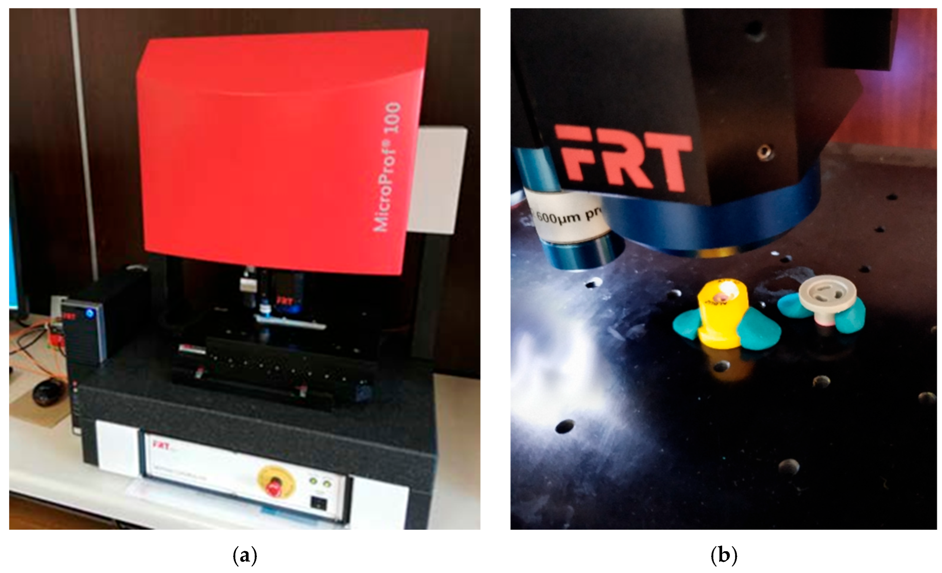
In order to prepare an accurate computer model of the nozzle, selected surfaces of the actual geometry were scanned. 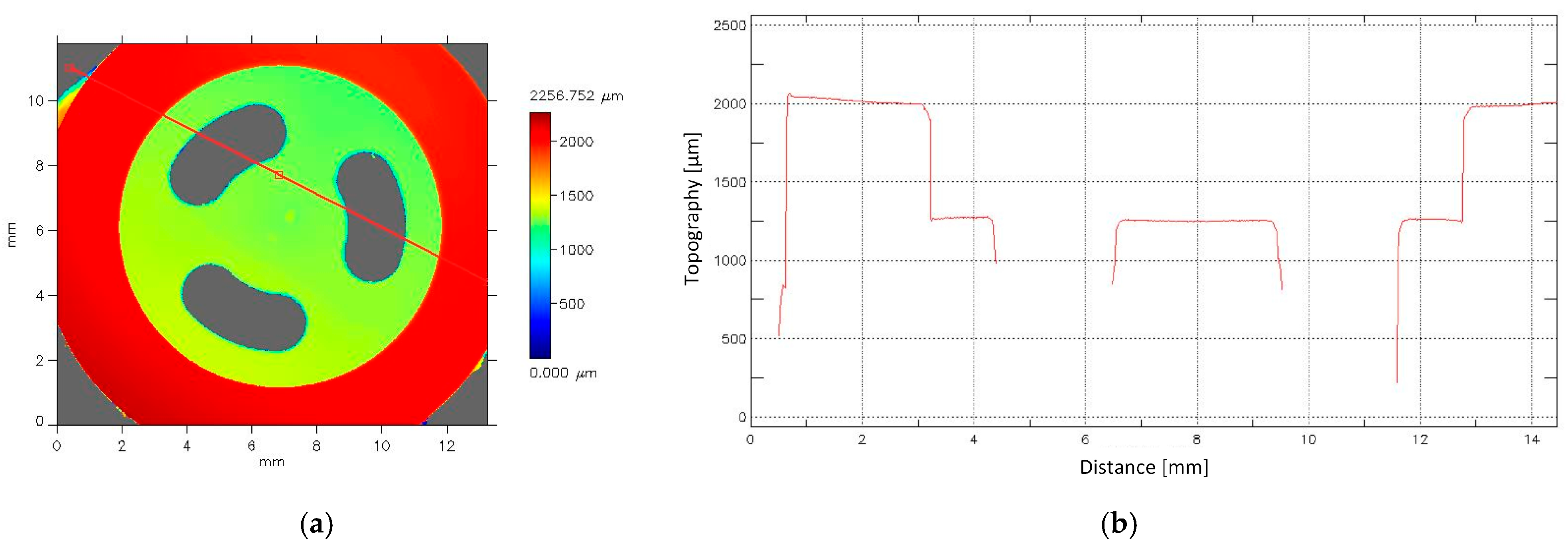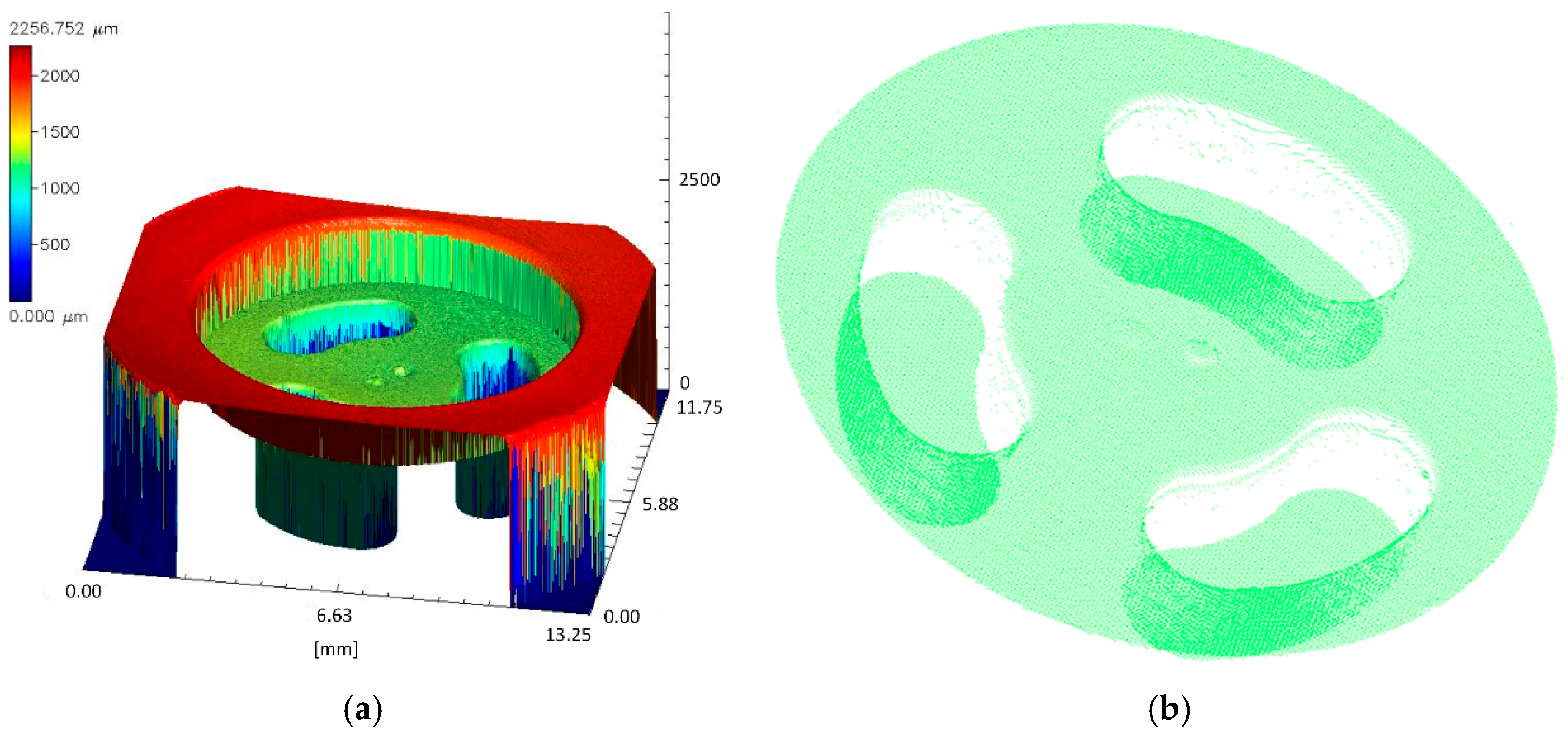The optical profilometer used for this was the FRT MicroProf 100 (Fries Research & Technology GmbH, Bergisch Gladbach, Germany), which makes it possible to measure the profile and surface roughness, flatness, and other parameters related to the profile and cross-section of the surface under examination using a non-contact optical method (Figure 2). The device enables vertical axis measurements up to 500 μm with an accuracy of 6 nm and up to 3 mm with an accuracy of 110 nm. The scanning conducted makes it possible to create 3D surface maps and 2D cross-sections (Figure 3). Due to its high measurement accuracy, the device allows for the evaluation of the surface roughness of the examined material (Figure 4).

The resulting point cloud was used to create a solid model in Catia V5-6R2021 software (Dassault Systèmes, Vélizy-Villacoublay, France). The points were imported into the Digitized Shape Editor module. This allowed the linear dimensions to be accurately mapped onto the sketch, and then a series of solid operations to be performed.

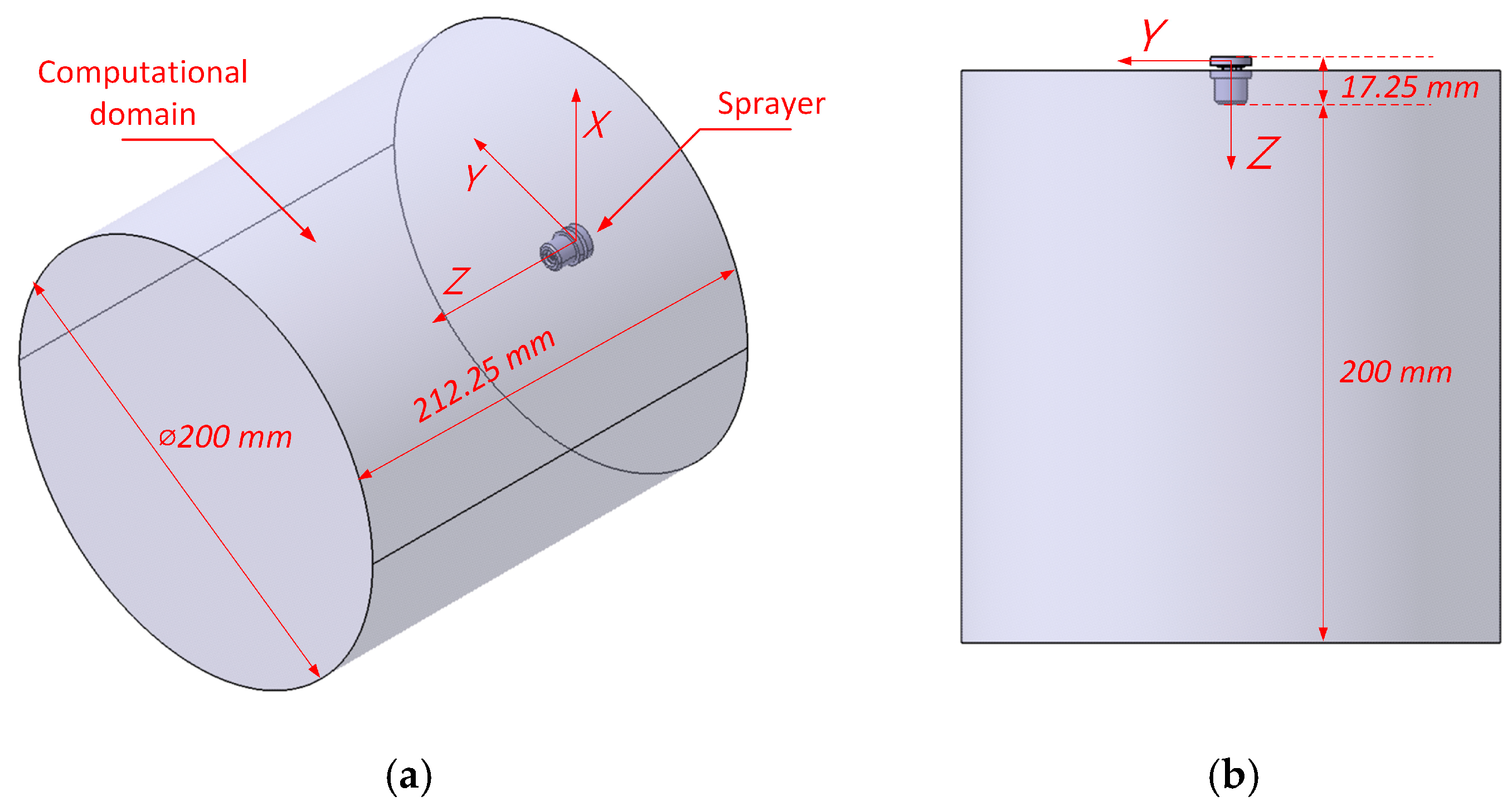
Based on the nozzle geometry created in the form of a solid model (Figure 5), work began on the flow model. For this purpose, the geometry was imported into Ansys 2024 software (Ansys, Inc., Canonsburg, PA, United States), where a computational domain was created (Figure 6), and a three-dimensional mesh was generated. The domain was in the form of a cylinder, on the base of which a sprayer was placed. The inlet area was the surface of the inlet to the modeled nozzle. The entire cylindrical surface of the computational domain and the bottom and top bases were defined as pressure outlets.

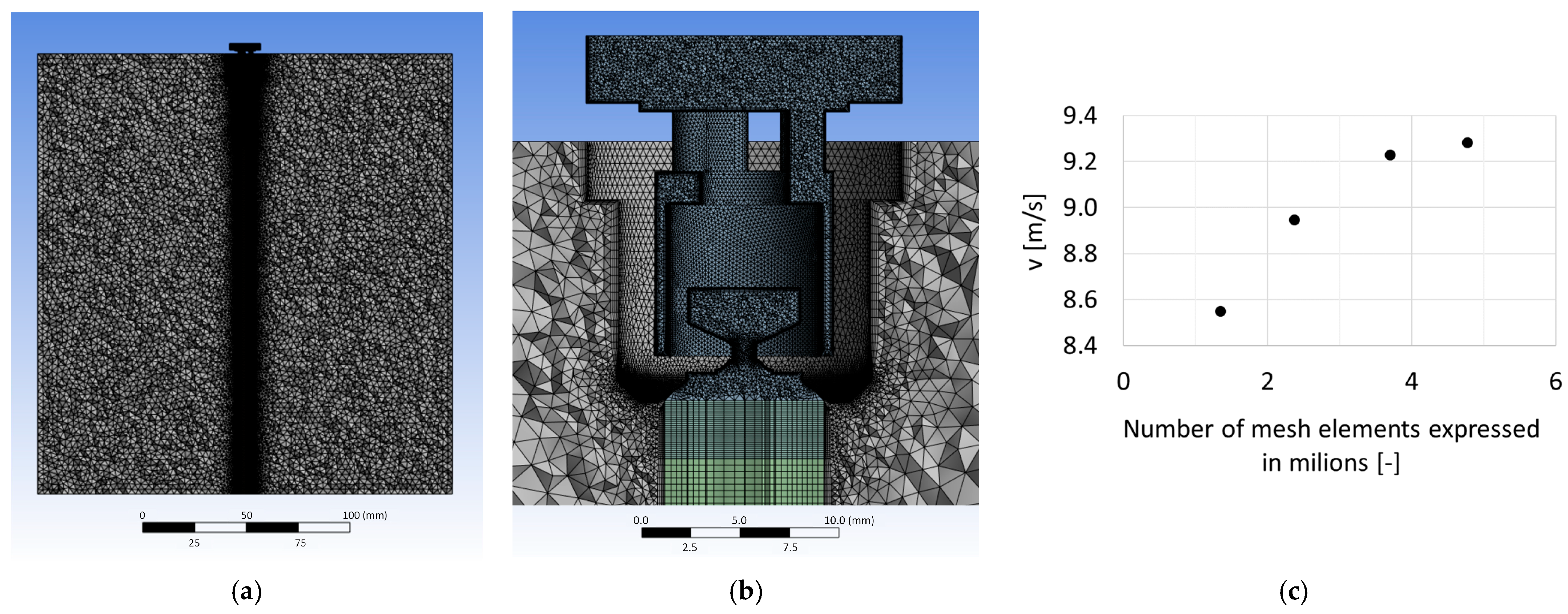
The developed mesh consisted of tetrahedral and hexahedral elements, comprising a total of 1,313,911 nodes and 4,783,050 elements. In areas with small cross-sections, element densification was applied. In addition, a boundary layer was created on the walls, using Inflation with Smooth Transition. The mesh size was determined by a mesh convergence study. The number of mesh elements was gradually increased, and the average velocity on the control surface passing through the nozzle outlet was observed (Figure 7c). A difference of 0.6% was noted between the adopted mesh and the previous one in terms of size. This value was considered satisfactory, and the final calculations were performed using the largest mesh among those analyzed. The tests showed that the number of elements achieved did not significantly impact the results, and further increasing it would only prolong the computation time. In regions with high-velocity gradients (e.g., in the swirl chamber and just beyond the outlet), further mesh refinement could improve the accuracy of phase interface representation and local turbulence; however, this would come at the cost of increased computational time. Figure 7 presents the computational mesh in two views. In the first view, the mesh of the entire computational domain is visible, while the second view shows the level of element densification, mainly within the internal volume of the nozzle. More complex shapes, particularly the internal volume of the atomizer, were meshed using tetrahedral elements. However, to ensure better control over the mesh density at the atomizer nozzle outlet, a subdomain in the form of a cylinder was created, extending from the atomizer to the end of the computational domain. Within this volume, a mesh based on hexahedral elements was applied. This is visible in Figure 7a as a refined core region of the domain.

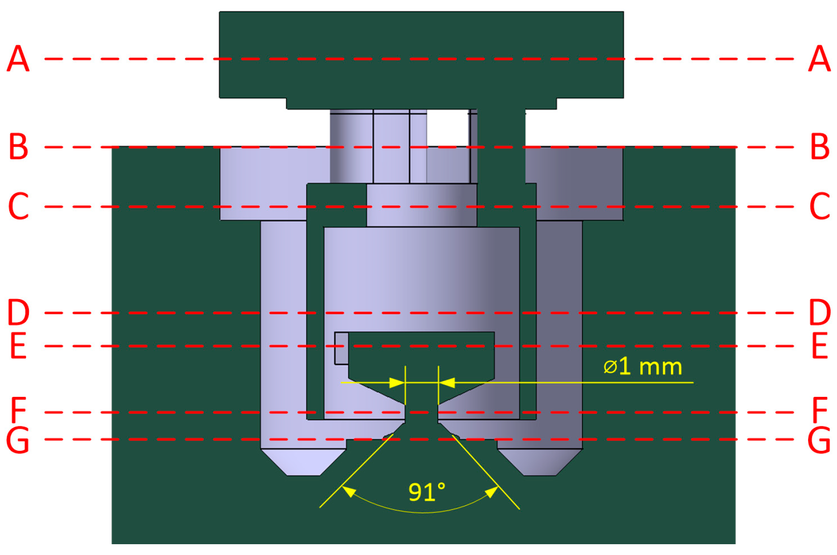
The horizontal cross-sections of the examined nozzle, for which the calculated parameter values were analyzed, are presented in Figure 8. The cutting planes, labeled sequentially as A-A, B-B, etc., were positioned at characteristic points of cross-sectional changes in the flow channel. The F-F plane is located in the exit orifice, with the smallest diameter of 1.18 mm. Defining the planes in this way was intended to analyze the average flow parameters in the individual nozzle sections. Selected parameters for the developed 3D computational model are shown in

Table 1. Selected parameters of the numerical model.

Boundary conditions
Fluids	Water (inlet), air (domain)
Inlet pressure	500,000 Pa (relative to ambient pressure)
Ambient pressure	101,325 Pa
Mass flow	0.010 kg/s
Water density	998.2 kg/m3
Water viscosity	1.003 × 10−3 kg1 m−1 s−1
Air density	1.225 kg/m3
Air viscosity	1.789 × 10−5 kg1 m−1 s−1
Physics models
Space	Three-dimensional
Time	Transient
Multiphase model	Volume of fluid (VOF)
Turbulence model	k-ω SST
Optional models	Gravity, pressure gradient force, two-way turbulence coupling, stochastic collision, coalescence, breakup
Eulerian phases
Water	Liquid, constant density
Air	Gas, constant density
Solution methods
Pressure–velocity coupling	SIMPLE scheme
Spatial discretization
Gradient	Least squares cell-based
Pressure	PRESTO!
Momentum	Second Order Upwind
Volume fraction	Geo-Reconstruct
Turbulent kinetic energy	First Order Upwind
Specific dissipation rate	First Order Upwind

. The calculations were performed in transient mode, indicating the variability of the analyzed parameters over time.

The model considers a gravitational acceleration of 9.81 m/s² directed along the vertical z-axis. The calculation solver was set as pressure-based due to the incompressible flow. The First Order Upwind scheme was used for the discretization of turbulent quantities (turbulence kinetic energy and specific dissipation rate) due to its robustness and stable convergence behavior. However, it is acknowledged that this choice introduces increased numerical diffusion, which may affect the resolution of turbulent structures and the accuracy of local turbulence parameters. The use of higher-order schemes, such as Second Order Upwind, will be considered in future studies to improve prediction quality in regions of high gradient flow. The multiphase model was the VOF method, with volume fraction parameters specified as explicit. It involves tracking the fraction of the volume of each phase in each computational cell. The fraction takes values from 0 to 1, where 0 means that the cell is completely filled with the first phase and 1 with the second phase. Intermediate values indicate that there is an interface between phases in the cell. For each phase, the transport equation for the volume fraction is solved. This equation characterizes the change in time and space of the proportion of a given phase in each cell.

In the VOF model, it is crucial to track the interfaces between the defined phases. This is done by solving the continuity equation that considers the volume fraction of the phases. For the j-th phase, the equation takes the Equation (1). On the other hand, the volume fraction equation for the primary phase is calculated based on Equation (2) [46].

$${\displaystyle \frac{1}{{\rho }_j}}\left[{\displaystyle \frac{\partial }{\partial t}}\left({\alpha }_j{\rho }_j\right)+\nabla \cdot \left({\alpha }_j{\rho }_j{\overline{v}}_j\right)\right]=S_{{\alpha }_j}+\sum _{i=1}^j\left({\dot{m}}_{ij}-{\dot{m}}_{ji}\right)$$

(1)

where ${\rho }_j$—density of the j-th phase; ${\alpha }_j$—fluid’s volume fraction of the j-th phase; ${\overline{v}}_j$—j-th phase velocity; $S_{{\alpha }_j}$—source term, the default value is 0; ${\dot{m}}_{ij}$—mass transfer from phase i to phase j; ${\dot{m}}_{ji}$—mass transfer from phase j to phase i.

$$\sum _{i=1}^j{\alpha }_i=1$$

(2)

As mentioned above, an explicit time formulation, which is time-dependent, was adopted in the calculations. The volume fraction is determined in a discrete manner using Equation (3).

$${\displaystyle \frac{{\alpha }_j^{n+1}{\rho }_j^{n+1}-{\alpha }_j^n{\rho }_j^n}{\Delta t}}V+\sum _f\left({\rho }_j{U}_f^n{\alpha }_{j,f}^n\right)=\left[S_{{\alpha }_j}+\sum _{i=1}^j\left({\dot{m}}_{ij}-{\dot{m}}_{ji}\right)\right]V$$

(3)

where $n+1$—index for new time step; $n$—index for previous time step; ${\alpha }_{j,f}$—face value of the j-th volume fraction; $U_f$—volume flux through the face, based on normal velocity; V—cell volume.

A sharp interface was chosen, which corresponds to models with a clearly defined interface between the phases. Two phases were defined: water and air. The surface tension coefficient for the interaction between the phases was 0.072 N/m, corresponding to the conditions for pure water. The use of pure water as the working fluid in this study was intended to create reference conditions for analyzing the fundamental mechanisms of two-phase flow in the conical nozzle. This approach allowed for minimizing the influence of additional chemical variables, such as adjuvants, which are commonly used in agriculture and, as mentioned in the introduction, significantly affect the surface tension of solutions. A continuum surface force model was chosen, which interprets the surface tension as a continuous, three-dimensional effect at the interface rather than as a boundary value condition at the interface. The inside of the domain was filled with air. A k-ω SST turbulence model was adopted with the production limiter option enabled.

At the inlet, a turbulence intensity of 1% and a turbulent viscosity ratio of 5 were set. Pressure–velocity coupling was defined using the SIMPLE algorithm. It uses the relationship between velocity and pressure corrections to enforce mass conservation and obtain a pressure field. For pressure discretization, the PRESTO! scheme was adopted, while the Geo-Reconstruct scheme, which is based on geometric information, was used for interface tracking. Under-relaxation factors for pressure and momentum were set at 0.5. The calculations were performed with a time step size of 10⁻⁵ s with 20 iterations per time step.

In this study, the VOF method was selected, as it enables a detailed representation of the formation and outflow of a liquid jet under two-phase water–air flow conditions. This method allows for accurate tracking of the phase interface by computing the volume fraction of each phase within individual mesh cells. Such capability is essential for precisely capturing the phenomena occurring during the initial stages of spraying, including the formation of the conical liquid jet, its acceleration, and the early phases of breakup.

An alternative approach would be to use the DPM, which is better suited for analyzing dispersed droplets moving through a continuous medium. However, the DPM requires prior specification of droplet size distribution, injection location, and velocity, which limits its applicability in cases where the goal is to model the continuous formation of the liquid jet and its dynamic interaction with the surrounding air.

The choice of the VOF method is, therefore, justified both by the nature of the investigated phenomenon and by the need to obtain detailed information about flow parameters across the entire nozzle geometry—without the need to impose additional assumptions regarding initial droplet characteristics. This approach enables a more accurate representation of real operating conditions and provides a solid foundation for further analysis of jet breakup and droplet dispersion in an extended spatial domain.

3. Results and Discussion

As a result of the 3D calculations performed in transient conditions, a range of parameters related to the liquid flow in the specified computational domain was obtained. The results are presented for an operating pressure of 500 kPa and a time of t = 15.64 ms, which elapsed since the liquid began entering through the defined inlet surface.

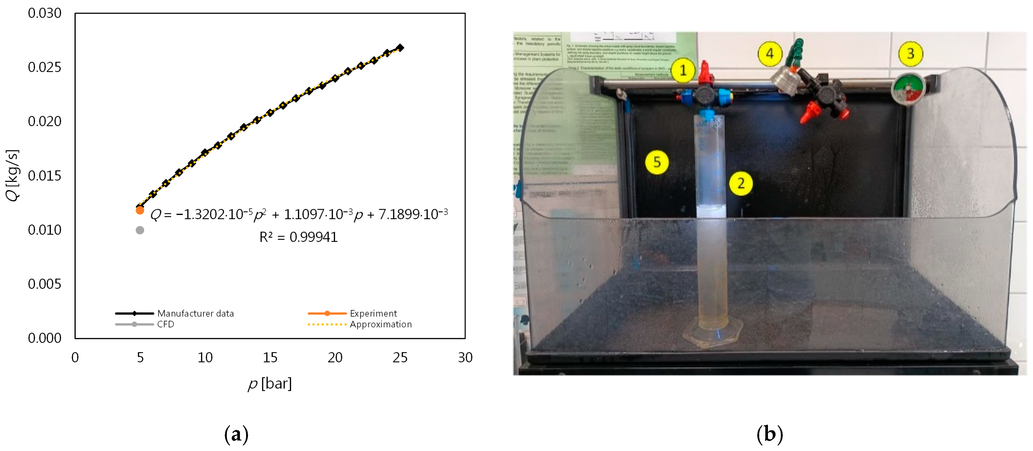
The mass flow rate of the nozzle as a function of operating pressure, as declared by the manufacturer, is presented in Figure 9. This parameter for the adopted working pressure was verified on an experimental test stand designed for visualizing the sprayed water jet (Figure 9). Measurements were conducted by the authors for the pressure value of 5 bar. The obtained experimental data were then compared with the manufacturer’s specifications to ensure consistency and validate the experimental setup.

The study involved measuring the outflow time of a specified liquid volume that flowed into a glass measuring cylinder. The resulting mass flow rate (0.012 kg/s) coincided with the manufacturer’s declared value. From numerical calculations for the tested geometry at an overpressure of 500 kPa, a mass flow rate of 0.010 kg/s was obtained. The observed difference from the nominal value of 16.7% can most likely be attributed to imperfections in the mapping of the nozzle geometry. A profilometer was used to identify complex shapes, while the remaining ones were measured with an ENGINDOT TACKLIFE DC02 digital caliper, offering a measurement accuracy of ±0.03 mm. In the solid model imported into the numerical model, sharp edges were defined in many places, which, for technological reasons, have rounded edges in reality. Another factor that may affect the observed differences could be inconsistencies in the initial conditions defined in the analysis, in particular, in terms of phase interactions compared to their actual progression. Detailed verification and validation procedures are crucial for ensuring the reliability of CFD simulations, especially those utilizing commercial software [48]. Therefore, the shape of the sprayed jet was also observed and compared with the jet obtained from numerical calculations.

The numerical results obtained, although generally consistent with experimental data and the nozzle’s catalog specifications, show certain discrepancies. A potential source of these deviations lies in the geometric representation of the nozzle. In the CAD model, locally idealized sharp edges were assumed, whereas the real component features smooth rounding due to manufacturing processes.

The use of transient simulation with a time step of 10⁻⁵ s allowed the capture of dynamic changes in the outlet region. However, the number of iterations per time step (20) and the applied discretization schemes may have limited the accuracy in resolving turbulent phenomena. The applied k-ω SST turbulence model with the production limiter is known for its good stability in near-wall flows, but its ability to capture complex vortex structures may be limited compared to more computationally intensive models such as large eddy simulation (LES) or detached eddy simulation (DES).

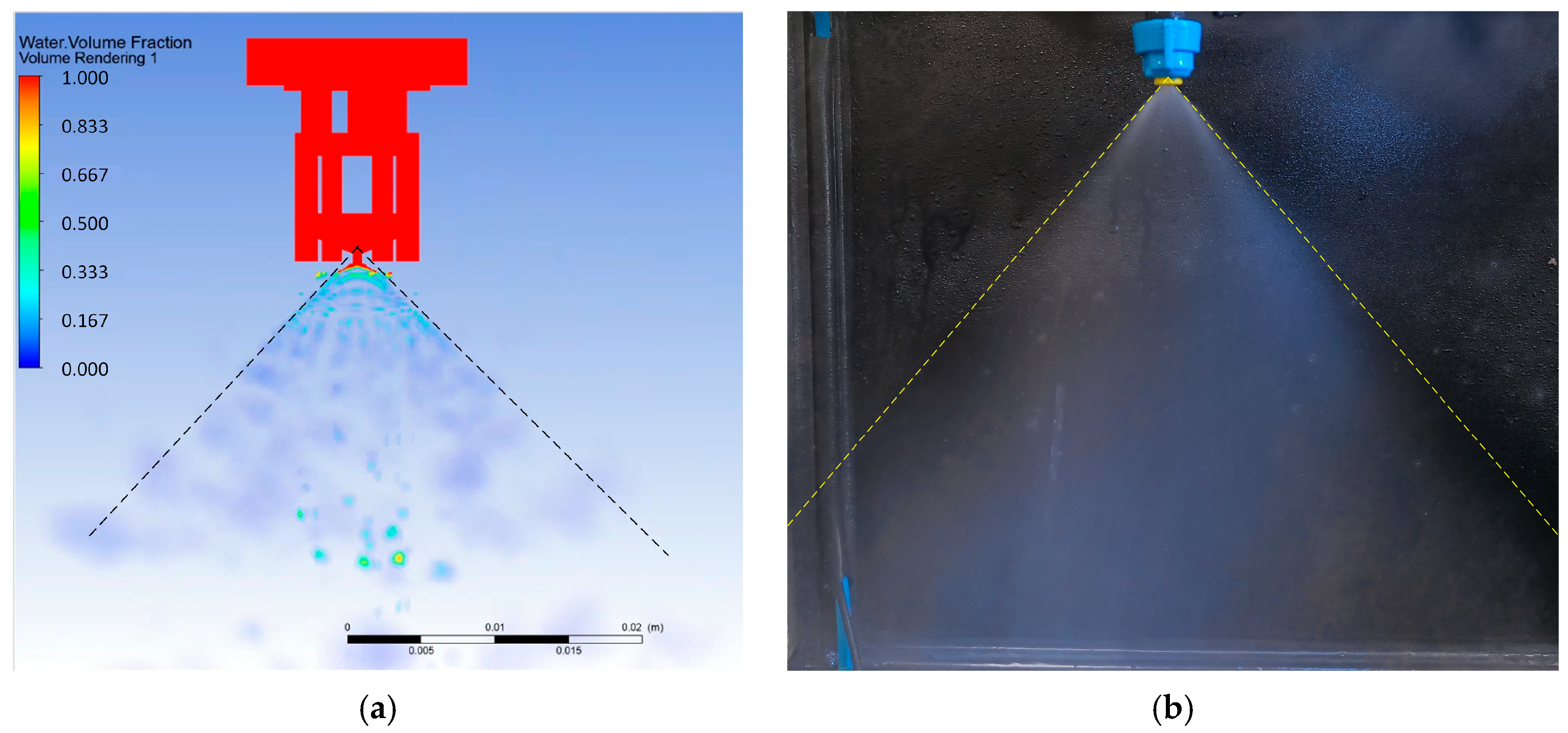
Figure 10 presents a comparison of the fluid jet obtained from CFD calculations and from experiments. The spray cone angle of the liquid on the test stand was consistent with the value specified by the manufacturer (80°). In the case of the liquid jet obtained from the numerical calculations, this angle was approximately 10% larger. This results from the complexity of the model factors related to the physics of the spraying process and the applied submodels that influence the equations characterizing multiphase flow.

The numerical calculations provided a distribution of key parameters related to the flow inside the computational domain, namely pressure and fluid velocity. In addition, thanks to the calculations performed with the VOF model, it was possible to obtain the water volume fraction distribution inside the air-filled domain. The last analyzed parameter was turbulence kinetic energy (TKE). This parameter was important because the sprayer contains a vortex insert, which significantly alters the flow parameters.

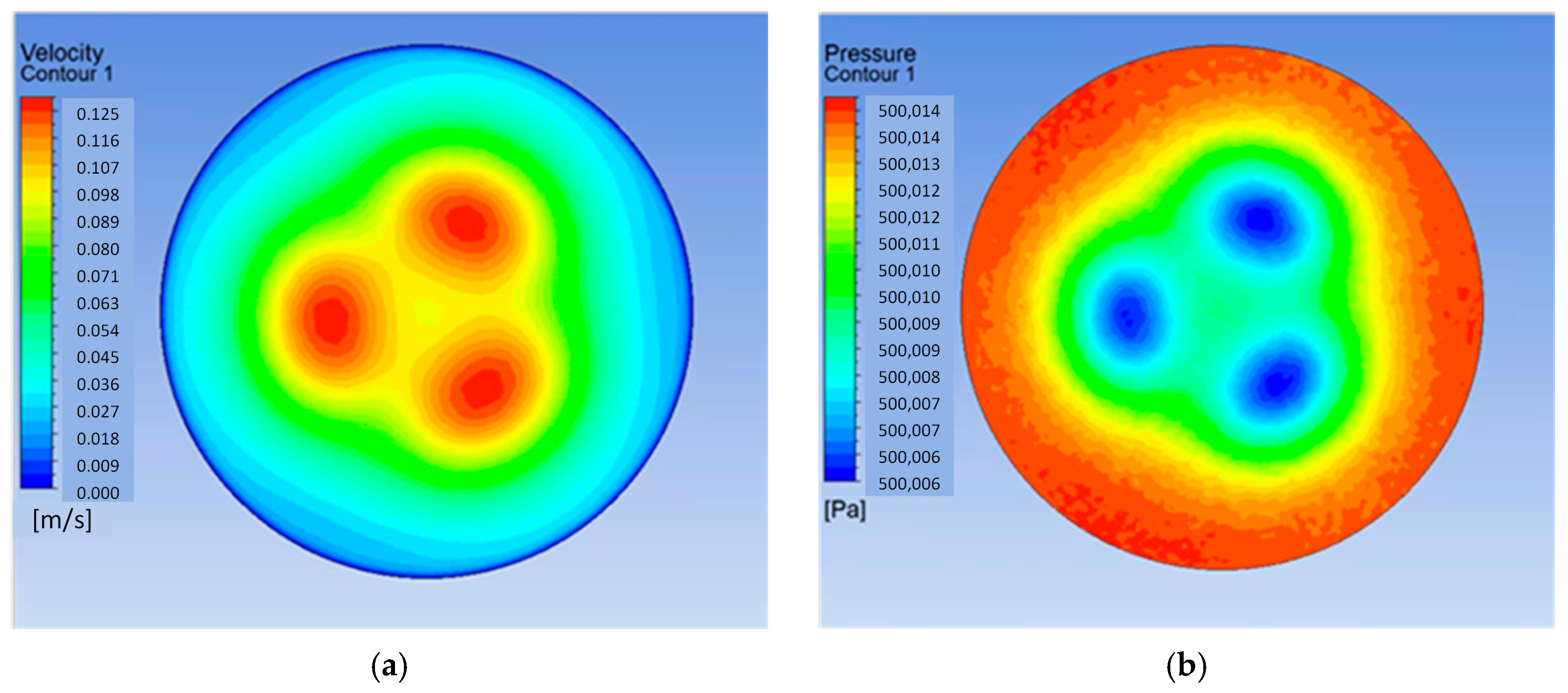
In the first part, selected parameter values for the defined horizontal cross-sections of the sprayer, as shown in Figure 8, were analyzed. The first of the A-A planes (Figure 11) corresponds to the cylindrical space directly behind the inlet surface. Behind the main inlet, the fluid accelerates toward three openings located on the disk with the stem, and in the A-A cross-section, the velocity reaches a value of 0.13 m/s. Inside this section, the pressure is almost exactly equal to the preset initial value of 500 kPa. A slight gradient reaching single pascals results from the gradual acceleration of the liquid toward the orifices.

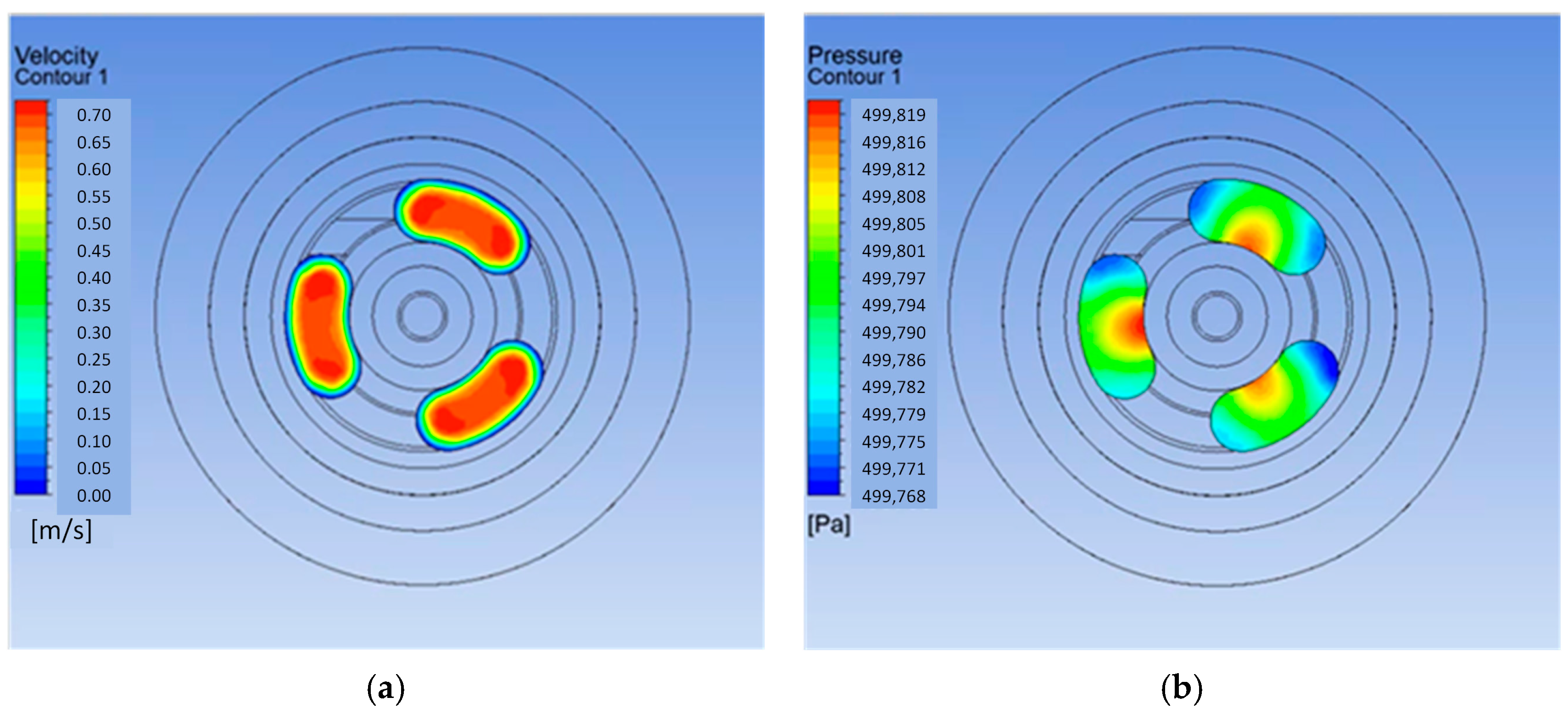
Another B-B section under consideration (Figure 12) corresponds to three kidney-shaped channels. The fluid flows through them in the direction of the annular chamber. A pressure drop of up to 232 Pa due to flow resistance was observed. At the walls of the holes, the velocity was close to zero due to the formation of the wall layer. In the middle of the hole, the velocity was still low at 0.70 m/s.

After flowing through the openings, the liquid flows into the annular chamber, which corresponds to the C-C plane (Figure 13). Its pressure was homogeneous at approximately 500 kPa, which corresponded to the inlet pressure. The velocity inside the chamber dropped slightly to a maximum value of approximately 0.60 m/s.

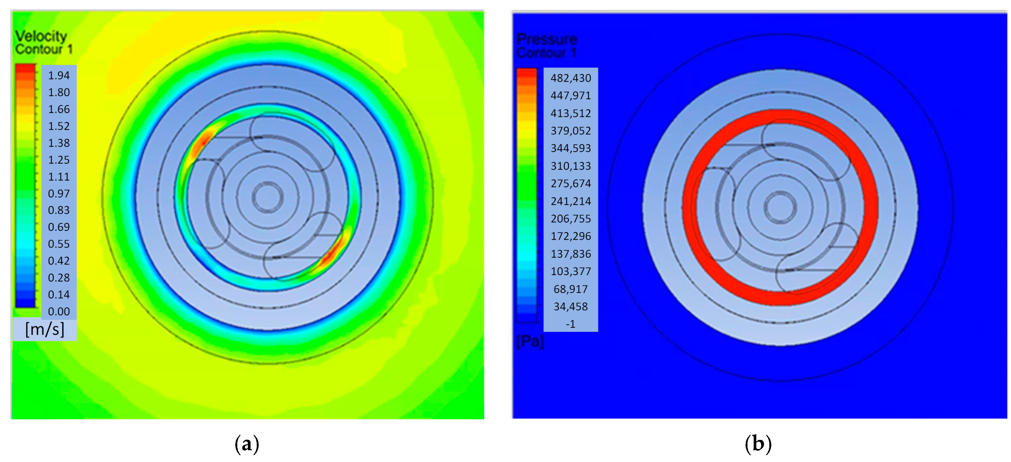
Further down the nozzle, the liquid moves towards the vortex insert. In the middle of the cylindrical channel (plane D-D in Figure 14), the velocity increases at two locations corresponding to the grooves in the vortex insert. The maximum value reached nearly 2 m/s. The static pressure did not change significantly and was approximately 500 kPa.

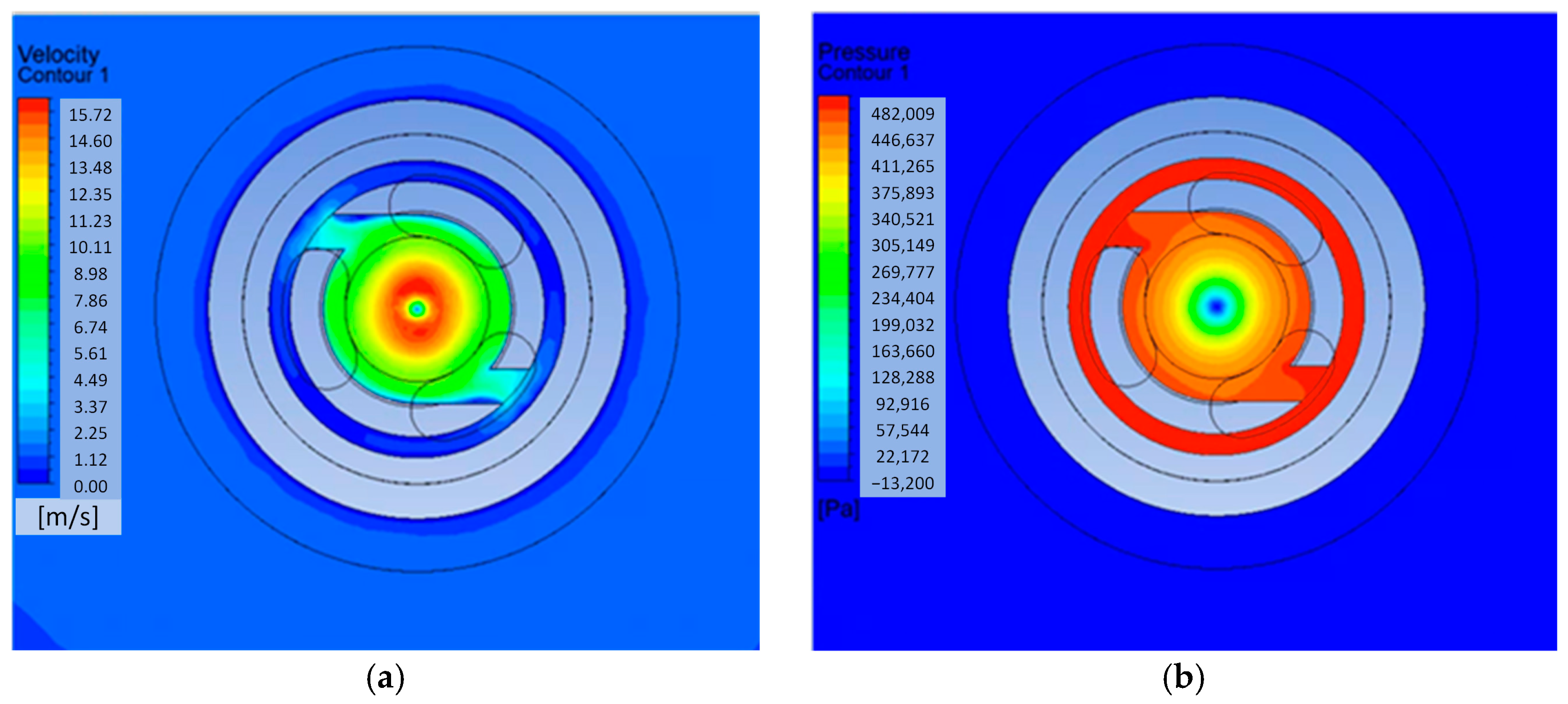
One particularly interesting area inside the nozzle is the vortex insert. The E-E plane runs through the center of the height of the outflow channels from this element (Figure 15). The shaping of the channels results in a significant acceleration of the fluid inside the chamber formed between the ceramic insert and the stem. Near the center of the chamber, the velocity is close to 16 m/s. It should be emphasized that in the very center, the velocity is half as low, measuring approximately 8 m/s. Due to the acceleration of the fluid, the static pressure decreases significantly, reaching negative values (below the accepted atmospheric pressure). The pressure dropped to approximately −13 kPa.

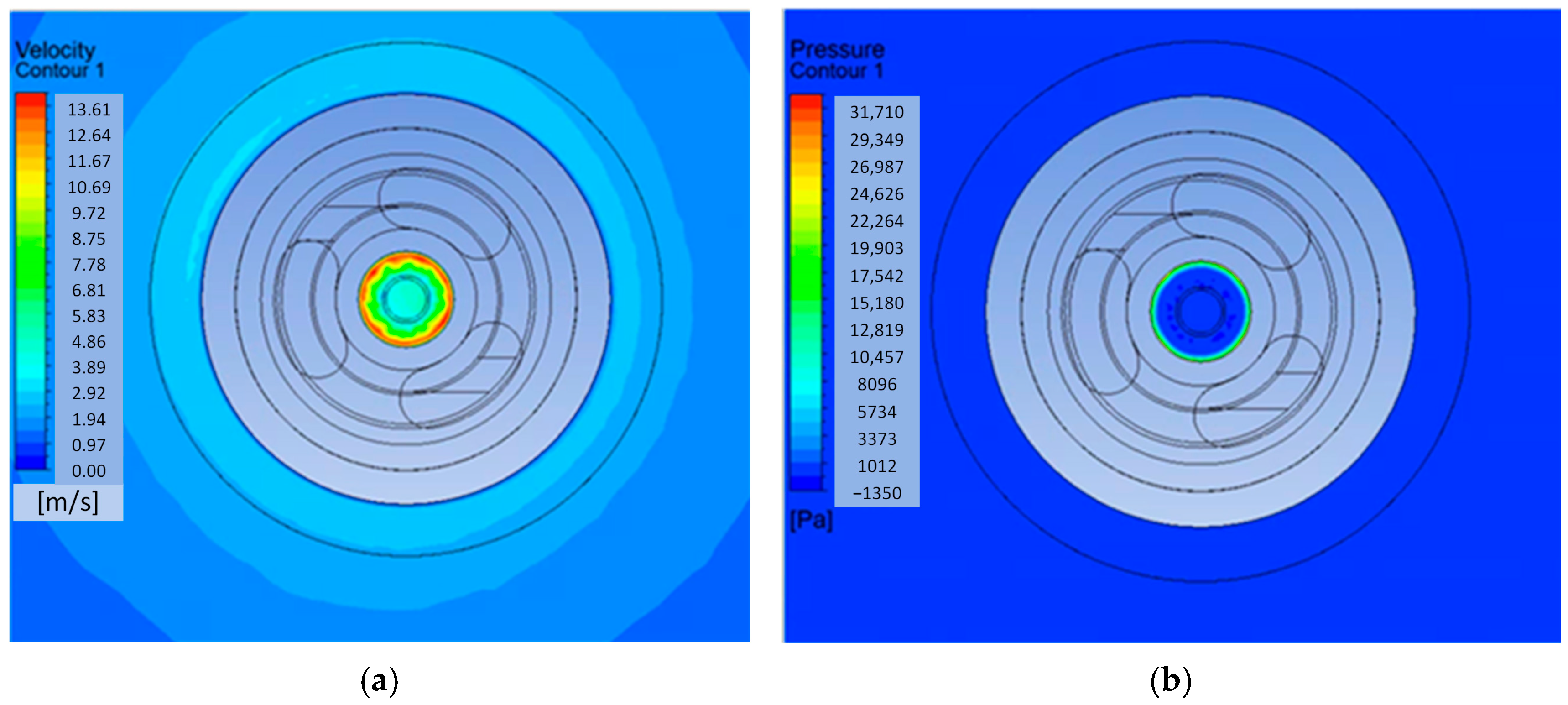
Next, the liquid flows into the orifice at the end of the sprayer, with a diameter of 1.18 mm. The pressure and velocity in the F-F plane corresponding to this location are shown in Figure 16. The water stream, pre-shaped in the vortex chamber, accelerates at the beginning of the orifice to a value exceeding 21 m/s. This value is achieved near the walls of the orifice. In the core of the flow, the velocity gradually decreases to a value close to zero. The acceleration of the fluid results in a pressure drop in accordance with Bernoulli’s principle. However, the negative pressure at the orifice inlet decreases from 13 kPa in the vortex chamber to 10 kPa.

The last of the considered G-G planes (Figure 17) runs just past the orifice outlet. As a result of the locally expanding diameter of the orifice, the velocity decreases to 13–14 m/s. Thus, the vacuum value is reduced to approximately 1 kPa. The velocity distribution is analogous to the distribution inside the orifice. This means that the highest velocity occurs at the perimeter of the jet with a circular cross-section. In the core, there is a gradual decrease in velocity to approximately 4 m/s.

The velocity profile shown in Figure 17 confirms the typical behavior of a hollow cone spray, with maximum velocity occurring along the perimeter of the jet and a central low-velocity region. This pattern results from the vortex insert geometry, which forces the liquid into a strong rotational motion along the nozzle walls. In practice, due to air entrainment and turbulent mixing, the central underpressure region is gradually reduced as the spray develops, and the axial velocity may increase in the core of the cone. This recovery is not fully captured by the current VOF model, which focuses on the near-field region. Future coupling with a DPM-based approach will allow a more accurate representation of particle dispersion and core flow reattachment in the far field.

The observed distributions of velocity, pressure, and turbulent kinetic energy (TKE) clearly indicate that the geometry of the investigated nozzle—particularly the presence of a ceramic vortex insert and a three-channel flow plate—plays a crucial role in shaping the internal flow. The lack of geometric symmetry, the presence of irregularly shaped channels, and the spiral guidance of the liquid through the swirl chamber promote the generation of strong angular momentum and intense vortex structures. As a result, the liquid jet accelerates more rapidly, and a localized pressure drop—consistent with Bernoulli’s principle—occurs in the outlet flow region.

Within the swirl chamber, the pressure gradient becomes intensified, generating a negative pressure reaching as low as −13 kPa. This is caused by centrifugal forces acting on the liquid as it follows spiral trajectories. Such conditions favor the local stretching of the liquid jet and facilitate its disintegration just after exiting the orifice. Additionally, the asymmetric arrangement of the inlet channels leads to a non-uniform velocity distribution along the jet perimeter. The observed velocity and TKE maxima near the outer edge confirm the formation of a characteristic hollow cone pattern, where the highest velocities are concentrated at the periphery of the spray while the central region maintains low pressure and limited flow.

From the perspective of spray engineering, such a configuration promotes the generation of fine droplets in the outer part of the cone, which can increase leaf surface coverage but, at the same time, creates a greater risk of droplet drift due to wind. In future work, it would be advisable to investigate the impact of changes in the geometry of the feed channels—including their number, angle of attack, and curvature—on the stability of the formed cone, the distribution of TKE, and the timing of spray breakup.

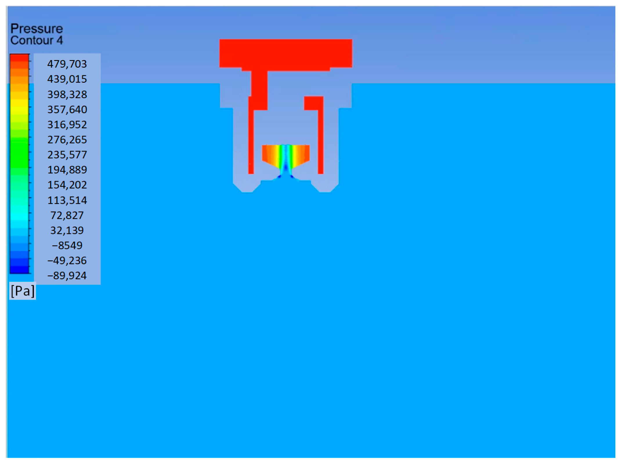
Figure 18 presents the pressure distribution inside the nozzle and in its immediate vicinity (at a distance of approximately 2 cm from the exit). A stable liquid flow through the nozzle was achieved after approximately 16 ms. The highest pressure gradient occurs in the chamber formed between the ceramic components: the vortex insert and the stem. As a result of the constriction at the nozzle exit, a rapid drop in pressure to less than ambient pressure is created. The obtained negative pressure was 90 kPa. However, just a few millimeters away from the nozzle exit, the pressure equalizes with the ambient pressure.

The analysis of the velocity distribution in the liquid outflow zone from the nozzle orifice, as shown in Figure 19, revealed more details. According to Bernoulli’s principle, due to the local narrowing of the flow in the orifice, the liquid accelerates rapidly and reaches a velocity exceeding 23 m/s. At the nozzle exit, a conical stream forms, with the highest velocities, ranging from 10 to 15 m/s, occurring in the outer region of the jet. The remainder of this zone has an irregular velocity field, varying in value over quite a wide range from 0 to 10 m/s. This is due to the turbulent nature of the flow and the local breakup of the continuous jet into droplets.

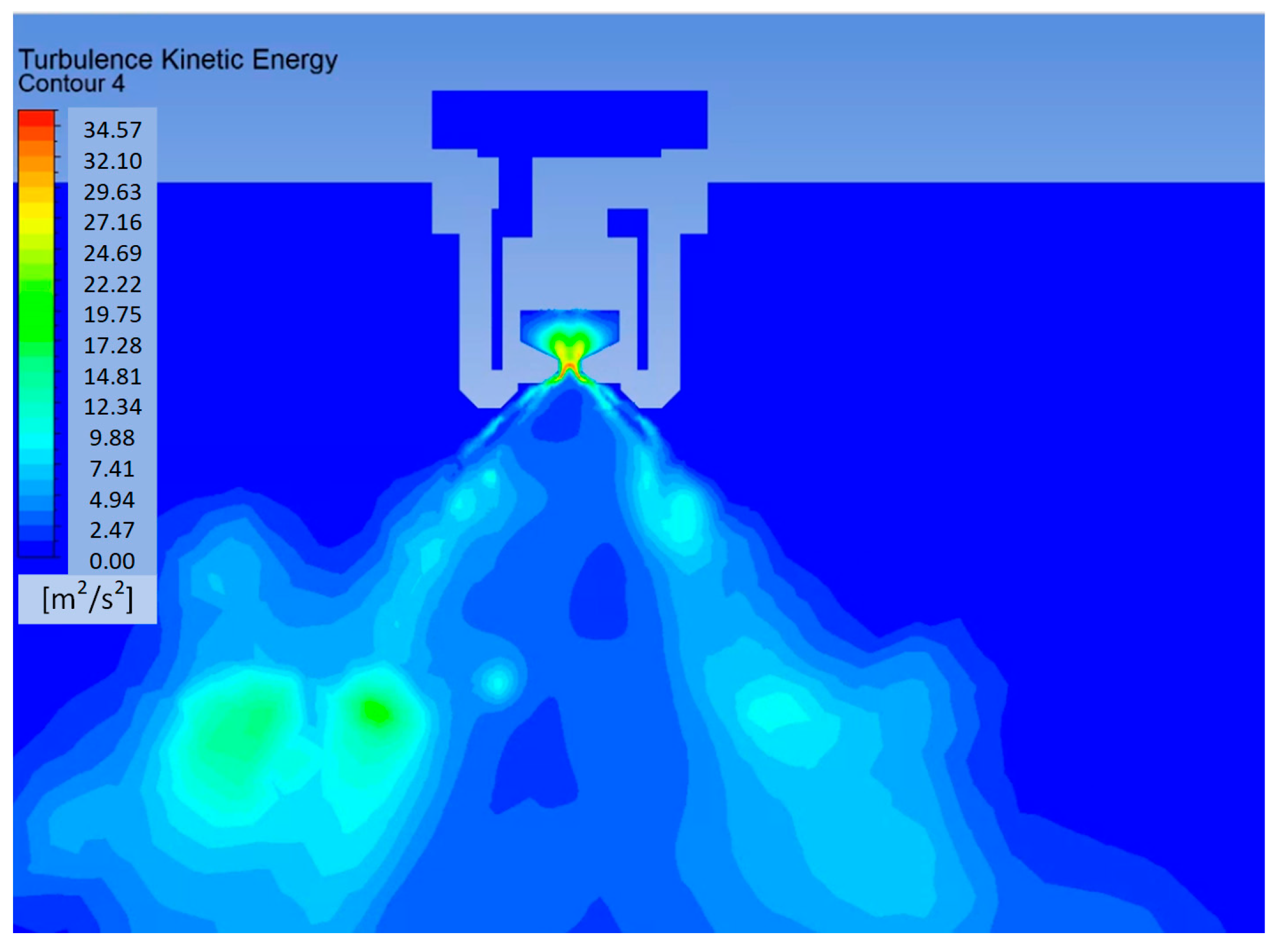
The last parameter analyzed was turbulence kinetic energy. The higher the TKE value, the more intense the velocity fluctuations and, therefore, the more turbulent the flow. In the context of a two-phase liquid spraying model in a gaseous atmosphere, this parameter indirectly indicates the intensity of phase mixing and particle dispersion. The maximum value of this parameter occurred at the exit of the discharge orifice and was 37.04 m²/s². In the zone directly behind the nozzle, a high variability in the TKE values was observed. The location of the maximum TKE values (10–15 m²/s²) approximately coincides with the regions of the highest velocity in this zone, as shown in Figure 20. This is due to the progressive breakup of the jet into droplets and the presence of local turbulence.

The maximum TKE values are concentrated near the outlet and along the periphery of the spray core, where strong shear layers develop due to the velocity difference between the swirling liquid jet and the surrounding air. These zones of elevated turbulence intensity are closely linked to the beginning of primary atomization, as high-speed shear promotes instability and fragmentation of the liquid film. Although breakup modeling was not included in the current simulation, the TKE distribution observed here aligns with the expected initiation sites of droplet formation.

Figure 21a–c shows the course of velocity, pressure, and turbulence kinetic energy strictly along the z-axis of the nozzle. The velocity along the chamber axis before the exit orifice (10–15 mm along the z-axis) reaches values from 6 to 11 m/s. Then, after exiting through the nozzle, it decreases to a low value of about 2 m/s. In this zone, the pressure becomes negative, i.e., it is below the ambient pressure. The intense fluid motion and local vortex phenomena resulting from the geometry of the vortex insert (presence of two inflow channels) result in achieving a high TKE value reaching up to 35 m²/s². Figure 21d–f present the obtained values of the analyzed parameters across the entire yz cross-sectional plane of the nozzle. The maximum velocity in the chamber before the exit nozzle reached nearly 25 m/s. Velocities reaching up to 10 m/s were achieved at a distance of 5 mm from this orifice (z = 20 mm). As the distance increased, the maximum value of this parameter decreased by approximately half to 5–6 m/s. Regarding pressure, its greatest fluctuation occurs in the region corresponding to the chamber before the exit orifice. At that point, the pressure decreases from a value of 500 kPa, close to the inlet value, to locally negative values. The maximum TKE values (approximately 35–36 m²/s²) correspond to those obtained directly on the z-axis. A local maximum at z = 34 mm, which is 19 mm from the exit orifice, deserves attention. At that point, this parameter reached a value close to 20 m²/s², which is twice the value observed in the rest of the outflow region. This may be the result of increased turbulence and phenomena associated with the breakup of the liquid stream into droplets.

4. Conclusions

The need for research on nozzles used in agricultural applications arises from the pursuit of increased efficiency in the process of applying plant protection agents (understood as saving the used substance and achieving better surface coverage) while reducing risks to the environment and human health. The numerical approach proposed in this study enables the modeling of the flow process and the initial formation of a liquid jet in this type of nozzle. This method allows for the verification of key parameters for various nozzle geometries without incurring the costs associated with preparing and conducting a series of experimental tests on a test stand.

The conducted research focused on a hollow cone nozzle designed for the application of plant protection agents in orchards and marked the beginning of analytical work on developing a comprehensive multiphase model combining water and air phases. The authors proposed a model that utilizes the VOF method. The distribution of flow-related parameters in selected sections of the computational domain was obtained. The analysis focused on the variation of velocity and pressure within the flow channels of the nozzle. The obtained results indicate that the critical area is the chamber at the nozzle exit, formed between the vortex insert and the ceramic stem. Along the longitudinal axis of the nozzle, the TKE value in this region reached 35 m²/s².

The cone angle of the spray differed by approximately 10% from the nominal value, while the mass flow rate differed by approximately 16.7%. These differences may be attributed to minor inaccuracies in the solid model representing the real nozzle geometry. A conical stream develops in the flow zone (several millimeters behind the sprayer orifice), where the outer region exhibits the highest velocities, attaining speeds between 10 and 15 m/s. Further away, the velocity decreases due to intensive mixing with the air. A significant impact on flow parameters is also exerted by various model settings related to turbulence, phase interaction, and mixing, as well as the physics of liquid jet breakup into droplets. This issue will be the subject of further analysis by the authors of this paper.

The obtained results and observed phenomena inside and just beyond the nozzle provide a solid foundation for continuing research aimed at improving the numerical model and expanding the analysis to additional aspects of the spraying process. In the next stages, models based on liquid jet breakup and individual droplet generation are planned—specifically, the use of the DPM combined with atomization submodels such as Kelvin–Helmholtz (KH) or Taylor analogy breakup (TAB). This will allow tracking the trajectories and velocities of individual droplets after leaving the nozzle and determining dispersion parameters in space.

The next step will involve introducing variable environmental conditions, such as wind speed, humidity, and temperature, enabling the simulation of spray drift and a better assessment of plant coverage efficiency under field conditions. Modeling droplet evaporation in flight, which significantly impacts crop protection effectiveness and environmental safety, may be particularly interesting.

From a design perspective, simulations of alternative nozzle geometry variants are also planned—for example, by changing the number and inclination angle of the holes in the swirl plate or modifying the geometry of the swirl insert. This will make it possible to identify configurations that promote greater stability of the liquid cone and a lower turbulence level.