Improved Electrochemical–Mechanical Parameter Estimation Technique for Lithium-Ion Battery Models

Abstract

Accurate and predictive models of lithium-ion batteries are essential for optimizing performance, extending lifespan, and ensuring safety. The reliability of these models depends on the accurate estimation of internal electrochemical and mechanical parameters, many of which are not directly measurable and must be identified via model-based fitting of experimental data. Unlike other parameter-estimation procedures, this study introduces a novel approach that integrates mechanical measurements with electrical data, with a specific application for lithium iron phosphate (LFP) cells. An error analysis—based on the Root Mean Square Error (RMSE) and confidence ellipses—confirms that the inclusion of mechanical measurements significantly improves the accuracy of the identified parameters and the reliability of the algorithm compared to approaches relying just on electrochemical data. Two scenarios are analyzed: in the first, a teardown of the cell provides direct measurements of electrode thicknesses and the number of layers; in the second, these values are treated as additional unknown parameters. In the teardown case, the electrochemical–mechanical approach achieves significantly lower RMSEs and smaller confidence ellipses, proving its superior accuracy and consistency. In the second scenario, while the RMSE values of electrochemical-mechanical model are similar to those of the purely electrochemical one, the smaller ellipses still indicate better consistency and convergence in the parameter estimates. Furthermore, a sensitivity analysis to initial guesses shows that the electrochemical-mechanical approach is more stable, consistently converging to coherent parameter values and confirming its greater reliability.

1. Introduction

Lithium-ion batteries (LIBs) have become the dominant energy storage technology for various applications, ranging from consumer electronics to grid storage and electric vehicles [1,2]. Accurate modeling of LIBs is essential for predicting performance, optimizing efficiency, and ensuring safe operation. Battery models can be broadly categorized into empirical, equivalent circuit models (ECMs) [3,4] and physics-based models [5]. The latter offers a more comprehensive representation of the multiphysics processes occurring in batteries; however, this increased accuracy comes at the cost of higher computational complexity due to the coupling of Partial Differential Equations (PDEs). Among physics-based models, the Doyle–Fuller–Newman (DFN) model [6] stands out as the most prominent due to its ability to accurately describe lithium-ion transport, charge transfer, and electrochemical reactions within the battery. It serves as a fundamental reference for advanced battery simulations and optimization studies, making it a cornerstone in battery modeling research. However, this requires the precise estimation of electrochemical and mechanical parameters, which influence battery behavior under operating conditions.

When it comes to battery modeling, it is important to distinguish between the manufacturer’s perspective and the end user or system integrator’s perspective. Manufacturers typically have access to comprehensive internal data, including detailed material properties, geometric specifications, and electrochemical parameters obtained through dedicated design, optimization, and characterization campaigns. In contrast, end users—such as developers of battery management systems or integrators of battery packs—often have limited access to such internal information. Therefore, parameter identification plays a crucial role in battery modeling, ensuring that simulation results align with actual behavior. Some parameters can be directly measured using experimental setups [7,8], while others are more challenging or expensive to determine, requiring estimation methods.

Many studies performed battery parameter estimation through voltage curve fitting [9,10,11], where experimental discharge and charge curves are matched to simulated ones. This method is widely used due to its simplicity and effectiveness in capturing electrochemical characteristics. The drawback is the reduced accuracy when dealing with a large number of parameters that are not strictly sensitive to the voltage profile—called “voltage-insensitive” after a dedicated sensitivity analysis [12]. Other works leverage the multi-objective approach in order to capture a larger number of sensitive parameters. COBRAPRO [13] is a MATLAB-based open-source toolbox with an integrated parameter estimation routine for physics-based battery models. It minimizes a multi-objective cost function considering the voltage profile and SOC depending on the concentration of lithium ions in the electrodes. PyBOP [14] is a Python library designed to work with PyBaMM, offering a flexible framework for parameter estimation. It uses both gradient-based and free derivative optimization methods to fit model parameters to experimental data, supporting custom objective functions. Zhang et al. [15] proposed a coupled electro-thermal model using Genetic Algorithms (GAs) and minimizing the multi-objective function through Pareto fronts.

Recently, significant focus has been placed on the mechanical response of LIBs during operation, leading to the development of various techniques to measure and model the reversible battery deformation induced by the electrochemical processes [16,17,18,19,20]. However, existing parameter estimation methods largely overlook this mechanical behavior. In this study, the effect of the mechanical measurements of the reversible battery deformation on parameter estimation is deeply investigated through an optimization model developed in COMSOL Multiphysics. Particularly focusing on LFP/graphite batteries, a comparison between the electrochemical and the electrochemical–mechanical approach is then presented to highlight the differences.

2. Materials and Methods

Optimization is an engineering challenge based on identifying the set of parameters ${\mathit{\theta }}^{\mathbf{\ast }}=\{{\theta }_1,\dots ,{\theta }_i,\dots ,{\theta }_n\}$ that minimize an objective function $f\left(\mathit{\theta }\right)$ while ensuring the constraints of the physical phenomenon (inequality $g_j\left(\mathit{\theta }\right)$ and equality $h_k\left(\mathit{\theta }\right)$ constraints). Each parameter ${\theta }_i$ can vary in a range defined between a lower bound $a_i$ and an upper bound $b_i$ in accordance with the parameter constraints. Therefore, an optimization problem is generally expressed with the mathematical formulation shown in Equation (1). The subscript i denotes the i-th parameter, j is used to indicate the j-th inequality constraint and k for the k-th equality constraint. The bold symbol $\mathit{\theta }$ denotes a parameter set, being a vector.

$$\left\{\begin{array}{c}Find{\mathit{\theta }}^{\mathbf{\ast }}:\hfill \\ f\left({\mathit{\theta }}^{\mathrm{\ast }}\right)\le f\left(\mathit{\theta }\right)\forall \mathit{\theta }\hfill \\ g_j\left(\mathit{\theta }\right)\le 0,j=1,\dots ,m\hfill \\ h_k\left(\mathit{\theta }\right)=0,k=1,\dots ,p\hfill \\ a_i\le {\theta }_i\le b_i,i=1,\dots ,n\hfill \end{array}\right.$$

(1)

The aim of this work is the introduction of a novel battery parameter estimation approach based on a multi-objective function that also integrates the reversible mechanical deformation of the battery during its operating conditions. To achieve this goal, it is necessary to develop an appropriate model that accurately describes the battery behavior and properly asses the optimization problem defining objective functions, parameters, and constraints as deeply described in this work. Optimization is performed using the BOBYQA algorithm [21], which is especially useful when the first derivative of the objective function is not available and each simulation is computationally expensive, requiring an efficient optimization strategy. A more detailed overview of the electrochemical–mechanical model and the optimization algorithm is provided in the following sections.

2.1. Doyle–Fuller–Newman Model

The DFN model provides a physics-based framework that captures the coupled electrical and chemical species transport phenomena that occur within the battery. Based on the porous electrode and concentrated solution theories, the model accounts for key processes such as lithium-ion diffusion in the solid and electrolyte phases and charge transfer kinetics at the electrode–electrolyte interface. It also captures the multiscale behavior arising from lithium diffusion within the active material particles. The DFN model is also referred to as the Pseudo-Two-Dimensional (P2D) model. This name arises from its formulation: it resolves a one-dimensional spatial domain along the electrode thickness, and at each position within this domain, it incorporates a second dimension representing lithium diffusion within spherical particles. The P2D governing equations and the corresponding boundary conditions are listed in

Table 1. Governing equations of the P2D model for LIBs. The subscripts n, p, and s indicate the negative electrode, positive electrode, and separator, respectively.

Description	Governing Equations	Boundary Conditions
Mass conservation
Active material particles, $k\in \{p,n\}$	${\displaystyle \frac{\partial c_{s,k}}{\partial t}}=\nabla ·\left[D_{s,k}^{\mathrm{eff}}({\displaystyle \frac{\partial c_{s,k}}{\partial r}}-{\displaystyle \frac{{\Omega }_k{c}_{s,k}}{R_{g}T}}{\displaystyle \frac{\partial {\sigma }_{h,k}}{\partial r}})\right]$	$D_{s,k}^{\mathrm{eff}}({\displaystyle \frac{\partial c_{s,k}}{\partial r}}-{\displaystyle \frac{{\Omega }_k{c}_{s,k}}{R_{g}T}}{\displaystyle \frac{\partial {\sigma }_{h,k}}{\partial r}}){|}_{r=0}=0,$ $D_{s,k}^{\mathrm{eff}}({\displaystyle \frac{\partial c_{s,k}}{\partial r}}{c}_{s,k}-{\displaystyle \frac{{\Omega }_k{c}_{s,k}}{R_{g}T}}{\displaystyle \frac{\partial {\sigma }_{h,k}}{\partial r}}){|}_{r=R_{p,k}}=-J_{Li,k}$
Electrolyte, $k\in \{p,s,n\}$	${ϵ}_{e,k}{\displaystyle \frac{\partial c_{e,k}}{\partial t}}={\displaystyle \frac{\partial }{\partial z}}\left(D_{e,k}^{\mathrm{eff}}{\displaystyle \frac{\partial c_{e,k}}{\partial z}}\right)+a_{s,k}(1-t_{+})J_{Li,k}$	${\displaystyle \frac{\partial c_{e,k}}{\partial z}}{|}_{z=0,t_p+t_s+t_n}=0$
Charge conservation
Active material particles, $k\in \{p,n\}$	${\displaystyle \frac{\partial }{\partial z}}\left({\sigma }_{s,k}^{\mathrm{eff}}{\displaystyle \frac{\partial {\mathrm{\Phi }}_{s,k}}{\partial z}}\right)=a_{s,k}F{J}_{Li,k}$	${\sigma }_{s,k}^{\mathrm{eff}}{\displaystyle \frac{\partial {\mathrm{\Phi }}_{s,k}}{\partial z}}){|}_{z=0,t_p+t_s+t_n}=F{J}_{Li,k},$${\sigma }_{s,k}^{\mathrm{eff}}{\displaystyle \frac{\partial {\mathrm{\Phi }}_{s,k}}{\partial z}}){|}_{z=t_p,t_p+t_s}=0$
Electrolyte, $k\in \{p,s,n\}$	${\displaystyle \frac{\partial }{\partial z}}\left[{\kappa }_{e,k}^{\mathrm{eff}}\left({\displaystyle \frac{\partial {\mathrm{\Phi }}_{e,k}}{\partial z}}-{\displaystyle \frac{2(1-t_{+})R_{g}T}{F}}{\displaystyle \frac{\partial ln\left(c_{e,k}\right)}{\partial z}}\right)\right]=-a_{s,k}F{J}_{Li,k}$	${\displaystyle \frac{\partial {\mathrm{\Phi }}_{e,k}}{\partial z}}{|}_{z=0,t_p+t_s+t_n}=0,$${\mathrm{\Phi }}_{e,k}{|}_{z=0,t_p+t_s+t_n}=0$
Reaction kinetics
Butler–Volmer	$J_{Li,k}=\left\{\begin{array}{cc}2{\displaystyle \frac{i_{0,k}}{F}}sinh{\displaystyle \frac{0.5F}{RT}}{\eta }_k\hfill & k\in \{p,n\}\hfill \\ 0\hfill & k=s\hfill \end{array}\right.$	-
Exchange current	$i_{0,k}=F{k}_k^{\mathrm{eff}}{\left[c_{e,k}{c}_{s,k}^{\mathrm{surf}}\left(c_{s,k}^{\max }-c_{s,k}^{\mathrm{surf}}\right)\right]}^{0.5}$	-
Overpotential $k\in \{p,n\}$	${\eta }_k(z,t)={\mathrm{\Phi }}_{s,k}(z,t)-{\mathrm{\Phi }}_{e,k}(z,t)-U_k-F{J}_{Li,k}{R}_{c,k}$	-

.

The superscript eff refers to the correction applied to the diffusion coefficients, conductivities, and reaction rates, accounting for porosity and tortuosity in each domain [22], as well as thermal dependence when the temperature differs from the reference value [23].

2.2. Mechanical Deformation

The electrodes of lithium-ion batteries are composed of porous composite structures that include active material particles, conductive additives, and a polymeric binder. The active material serves as a host for lithium ions, which are reversibly inserted and extracted during charge and discharge. These processes are called intercalation and deintercalation, respectively. As lithium ions intercalate into or deintercalate from the host structure, they cause lattice configuration changes, leading to microscopic volume expansion or contraction.

The lattice structure strain can be characterized through XRD techniques by measuring the variation of the lattice parameters as a function of the corresponding state of lithiation of the electrode. The state of lithiation is the ratio between the actual and the maximum amount of lithium concentration that can be hosted from the active material (y is the cathode state of lithiation, while x is the anode one, as reported in Equation (2)).

$$y={\displaystyle \frac{c_{s,p}}{c_{s,p}^{max}}};x={\displaystyle \frac{c_{s,n}}{c_{s,n}^{max}}}$$

(2)

The maximum lithium concentration depends on the lithiated active material crystal’s density ${\rho }^{crystal}$ and molar mass $M_m$, as shown in Equation (3) [24].

$$c_{s,k}^{max}={\displaystyle \frac{{\rho }_k^{crystal}}{M_{m,k}}}$$

(3)

During lithiation, active materials exhibit phase transitions from their delithiated configuration to the fully lithiated one. LFP undergoes a single phase transition from FePO₄ to LiFePO₄. In contrast, graphite (C₆) manifests multiple phase transitions before reaching its fully lithiated stage LiC₆ [16,25]. In addition, graphite’s stage transition is not symmetric during its lithiation–delithiation cycle. This is mainly due to the presence of stage IIL during lithium extraction. In fact, this stage is only present at low discharge current rates and gradually fades, increasing the discharge current. Therefore, there is a lithiation window where stages II, IIL, and III coexist; lower discharge rates increase the stage IIL volume fraction and smooth the volume change from stage II to III due to the lower density of stage IIL. Using the XRD measurement of LFP [26] and graphite [25,27], the crystal volume changes as function of the state of lithiation are shown in Figure 1.

The lattice parameters exhibit directional dependence in their deformation due to the intrinsic anisotropy of the lattice structure. However, this anisotropic nature is mitigated by the random orientation of the crystals within the particle. Thus, considering the volumetric strain, the active material particle deforms consistently with its crystal lattice.

Then, at the upper scale, the electrode volume change $\Delta V^e$ depends on the $n^p$ particles’ volumetric deformation $\Delta V^p$ and on a possible reduction in porosity accounted for through a volumetric expansion parameter $\upsilon$ [28], as shown in Equation (4). In addition, the volume of the $n^p$ particles constitutes the overall active material volume, leading to Equation (5).

$$\Delta V^e=\upsilon n^p\Delta V^p$$

(4)

$$n^p{V}_0^p=\zeta V_0^e$$

(5)

Therefore, the volumetric strain of the electrode is obtained by dividing the Equation (4) by the initial volume of the single particle $V_0^p$ and accounting for Equation (5), as reported in Equation (6). Since the battery is assumed to be free to expand, the reduction in porosity is considered negligible, adopting the assumption of $\upsilon =1$ [16].

$${\epsilon }_v^e\left(t\right)={\displaystyle \frac{\Delta V^e}{V_0^e}}=\zeta {\displaystyle \frac{\Delta V^p}{V_0^p}}=\zeta {\epsilon }_v^p\left(t\right)$$

(6)

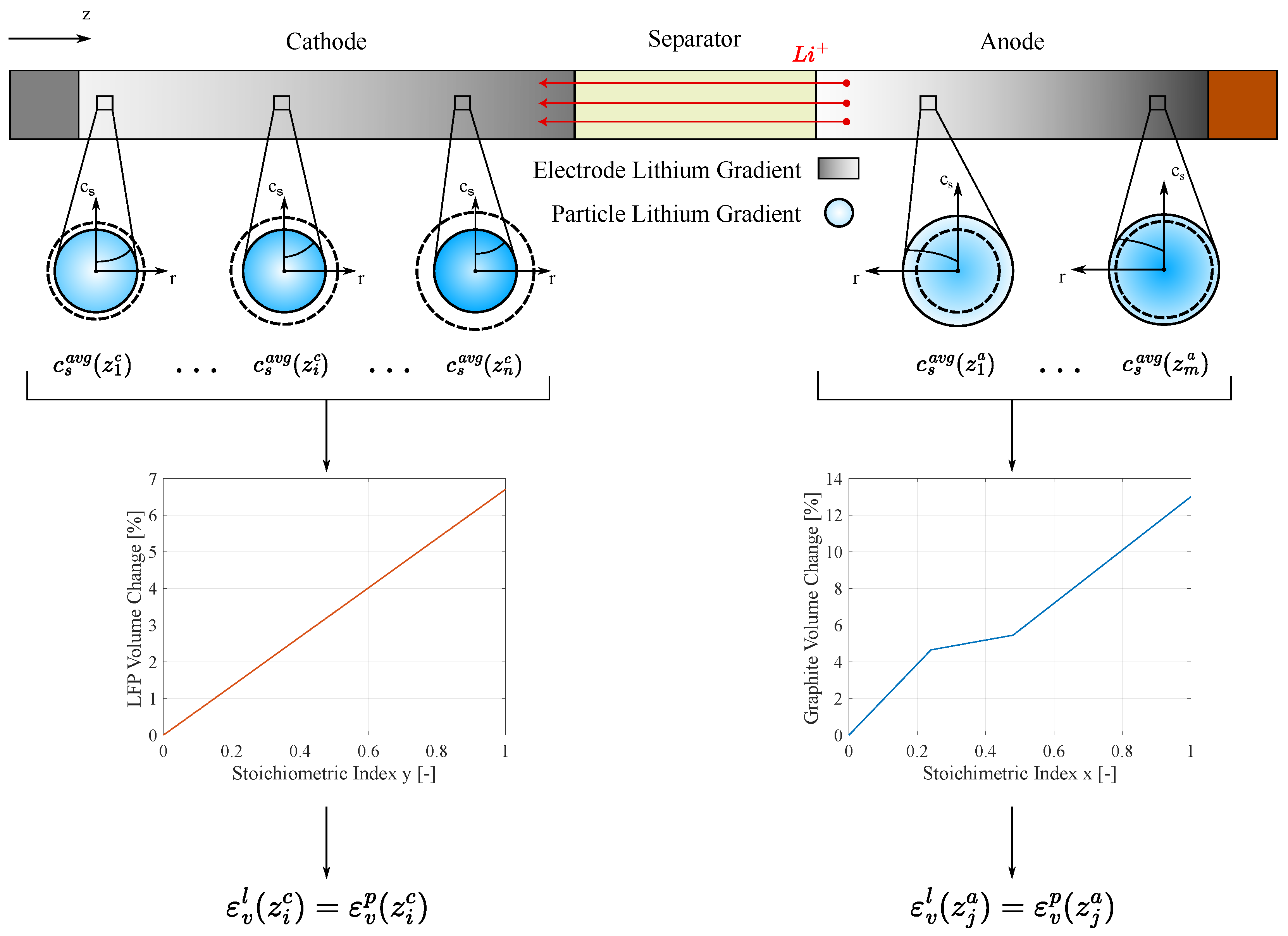
The previous equations hold under the assumption that all $n^p$ particles deform uniformly. However, this is not entirely accurate due to lithium diffusion across the electrode thickness. In reality, during battery operation, the lithiated electrode has more lithium content near the separator, while the delithiated electrode has a higher lithium concentration near the current collector. In fact, the diffusion of lithium ions is less constrained in the separator area (Figure 2).

Equation (6) remains valid if ${\epsilon }_v^p\left(t\right)$ represents the average deformation of the particles across the electrode thickness. To achieve this, the P2D model is used to extract the lithium concentration $c_s(z,r,t)$ at different positions in this direction. The concentration is then averaged over the particle radius ($c_s^{avg}(z,t)$) to determine the crystal lattice strain of the material, and consequently the particle strain ${\epsilon }_v^p\left(c_s^{avg}(z,t)\right)$, as shown in Figure 2. Finally, the particle strain is averaged across the electrode thickness to obtain the overall mean particle deformation ${\epsilon }_v^p\left(t\right)$.

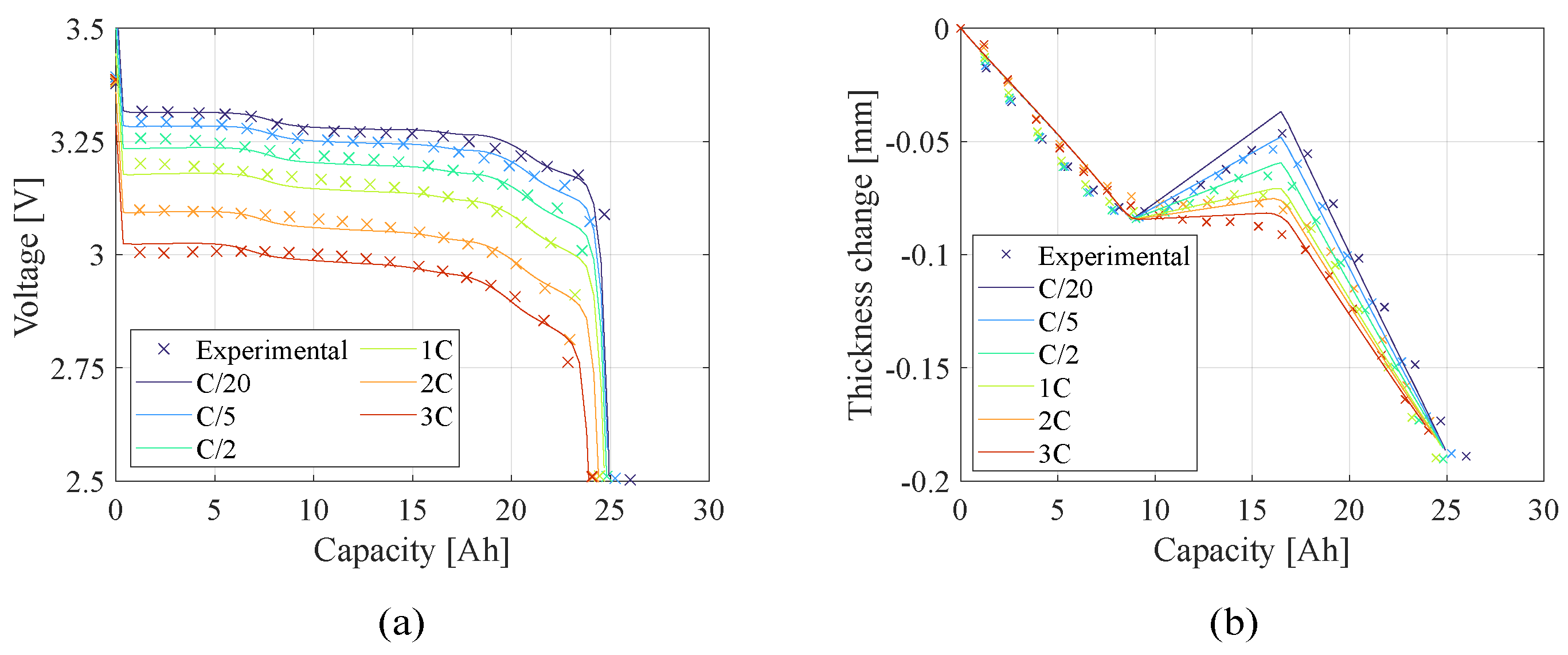
The volumetric strain propagates across the battery scales, resulting in a macroscopic thickness change that is evaluated by accounting for the deformation of both the electrodes and the presence of N layers [29,30]. Due to the thinness of the electrode with respect to in-plane geometry, the volumetric strain of the electrode is assumed to be responsible for just the out-of-plane strain (${\epsilon }_z^e={\epsilon }_v^e$) [16], resulting in the overall battery thickness change modeled as presented in Equation (7).

$$\Delta t_{bat}\left(t\right)=N(t_p{\epsilon }_{z,p}^e\left(t\right)+t_n{\epsilon }_{z,n}^e\left(t\right))$$

(7)

2.3. Objective Function

Once the electrochemical–mechanical behavior of the battery is modeled, the objective function for the parameter estimation can be set. Least-Square Objective Function (LSOF) was used to measure and minimize the difference between observed data points and the model’s predicted values. This approach is very useful for curve fitting since it evaluates the sum of squared errors computed over all data points, preventing positive and negative errors from canceling out and ensuring that larger deviations are penalized more heavily, improving convergence.

In a time-dependent curve fitting, considering $u_i$ the generic variable at the i-th time step, the $LSOF$ is computed, as presented in Equation (8).

$$LSOF\left(\mathit{\theta }\right)=\sum _{i=0}^n{(u_i^{mod}\left(\mathit{\theta }\right)-u_i^{exp})}^2$$

(8)

A multi-objective function approach is needed to evaluate the integration of the battery deformation in parameter estimation. Therefore, two LSOFs need to be computed in order to account for both the electrochemical measurements of the voltage profile and the mechanical measurements of the battery deformation.

$$LSO{F}_{ec}\left(\mathit{\theta }\right)=\sum _{i=0}^n{(V_i^{mod}\left(\mathit{\theta }\right)-V_i^{exp})}^2$$

(9)

$$LSO{F}_m\left(\mathit{\theta }\right)=\sum _{i=0}^n{(\Delta t_{bat,i}^{mod}\left(\mathit{\theta }\right)-\Delta t_{bat,i}^{exp})}^2$$

(10)

Due to the different scales of the electrochemical objective function $LSO{F}_{ec}$ and the mechanical one $LSO{F}_m$, Equations (9) and (10) have been normalized with respect to the square of the minimum voltage and maximum deformation (measured at the end of the test), respectively. Additionally, the battery capacity C is controlled with the same quadratic approach, obtaining the objective functions reported in Equations (11)–(13) which constitute the multi-objective problem statement presented in Equation (14) as a vector of objective functions.

$$f_{LSO{F}_{ec}}\left(\mathit{\theta }\right)={\displaystyle \frac{LSO{F}_{ec}\left(\mathit{\theta }\right)}{V_{min}^2}}$$

(11)

$$f_{LSO{F}_m}\left(\mathit{\theta }\right)={\displaystyle \frac{LSO{F}_{ec}\left(\mathit{\theta }\right)}{\Delta t_{max}^2}}$$

(12)

$$f_C\left(\mathit{\theta }\right)={\displaystyle \frac{{(C^{mod}\left(\mathit{\theta }\right)-C^{exp})}^2}{{\left(C^{exp}\right)}^2}}$$

(13)

$$\mathit{F}\left(\mathit{\theta }\right)=\left\{\begin{array}{c}{f}_{LSO{F}_{ec}}\left(\mathit{\theta }\right)\\ f_{LSO{F}_m}\left(\mathit{\theta }\right)\\ f_C\left(\mathit{\theta }\right)\end{array}\right\}$$

(14)

Depending on the same set of parameters $\mathit{\theta }$ from the same multiphysics modeling, the objective functions cannot be minimized at the same time and independently. Therefore, the multi-objective problem is solved using a scalarization approach to reduce computational complexity and enable variations in the weighting of the objective functions with respect to the Pareto technique [31,32]. Thus, a single objective function is obtained in Equations (15) and (16), where $\mathit{w}$ is the weights vector of the objective functions. Weighting factors are eventually applied to prioritize certain objective functions over others. The electrochemical-only parameter estimation $w_2=0$ is used to ignore the mechanical objective function.

$$f\left(\mathit{\theta }\right)={\mathit{w}}^T·\mathit{F}\left(\mathit{\theta }\right)$$

(15)

$$f\left(\mathit{\theta }\right)=w_1{f}_{LSO{F}_{ec}}\left(\mathit{\theta }\right)+w_2{f}_{LSO{F}_m}\left(\mathit{\theta }\right)+w_3{f}_C\left(\mathit{\theta }\right)$$

(16)

2.4. Optimization Algorithm

Since the optimization problem involves multiple objectives, the derivative of $f\left(\mathit{\theta }\right)$ with respect to the control variables is not easily obtainable: the presence of several objectives complicates the calculation of a unique and continuous gradient, making gradient-based algorithms unsuitable. In addition, changes in geometry often lead to remeshing, which may introduce discontinuities or non-differentiable behavior in the objective function. As a result, the computed gradients may be inaccurate or undefined. Therefore, a derivative-free algorithm is more appropriate for addressing this type of problem. The drawback is the slower convergence of the optimization process.

Among the derivative-free algorithms implemented in COMSOL Multiphysics, BOBYQA (Bound Optimization BY Quadratic Approximation) is the only one that uses a quadratic interpolation model to approximate the objective function. Unlike gradient-based methods, BOBYQA constructs and updates a local quadratic model $Q\left(\mathit{\theta }\right)$ using only objective function evaluations. In particular, the quadratic model is built to interpolate the objective function at a set of m interpolation points $\{{\mathit{\theta }}_{\mathbf{1}}\dots ,{\mathit{\theta }}_{\mathit{j}},\dots ,{\mathit{\theta }}_{\mathit{m}}\}$, with $m\ge n+1$, as shown in Equation (17), where ${\mathit{\theta }}_{\mathit{j}}$ indicates the j-th parameter set. The interpolation points are strategically chosen and updated, as stated by Powell in his work [21].

$$Q\left({\mathit{\theta }}_{\mathit{j}}\right)=f\left({\mathit{\theta }}_{\mathit{j}}\right),\forall j=1,\dots ,m$$

(17)

Then, the quadratic approximation of the objective function has the form presented in Equation (18), where c is a scalar constant, $\mathbf{g}$ is the estimated gradient, $\mathcal{H}$ is an approximated Hessian matrix, and ${\mathit{\theta }}_{\mathbf{k}}$ is the evaluation point at the k-th iteration.

$$Q\left(\mathit{\theta }\right)=c+\mathit{g}(\mathit{\theta }-{\mathit{\theta }}_{\mathit{k}})+{\displaystyle \frac{1}{2}}{(\mathit{\theta }-{\mathit{\theta }}_{\mathit{k}})}^T\mathcal{H}(\mathit{\theta }-{\mathit{\theta }}_{\mathit{k}})$$

(18)

To determine the next point to evaluate, BOBYQA minimizes the quadratic model $Q\left(\mathit{\theta }\right)$ within a neighborhood of the current point ${\mathit{\theta }}_{\mathit{k}}$, known as the trust region. This area is defined by a radius ${\delta }_k$, which bounds the maximum allowed step from the current iteration. The trust-region subproblem is expressed in Equation (19).

$$\underset{\mathit{\theta }\in {\mathcal{D}}_k}{min}Q\left(\mathit{\theta }\right){\mathcal{D}}_k=\{\mathit{\theta }\in {\mathbb{R}}^n,\parallel \mathit{\theta }-{\mathit{\theta }}_{\mathbf{k}}\parallel \le {\delta }_k\}$$

(19)

After evaluating the objective function at the new candidate point, the radius ${\delta }_k$ is updated depending on the agreement between the predicted decrease in $Q\left(\mathit{\theta }\right)$ and the actual decrease in $f\left(\mathit{\theta }\right)$. If the model prediction is sufficiently accurate, ${\delta }_k$ is expanded to allow broader exploration; otherwise, it is reduced to focus on a more local region, enhancing model reliability but risking the possibility of missing the global minimum. In parallel, the quadratic model itself is updated to maintain interpolation accuracy: whenever a new function evaluation is accepted and one of the existing interpolation points is replaced, the curvature of the model—represented by the Hessian approximation $\mathcal{H}$—must also be updated. This update ensures that the new model still satisfies the interpolation conditions at the updated set of points.

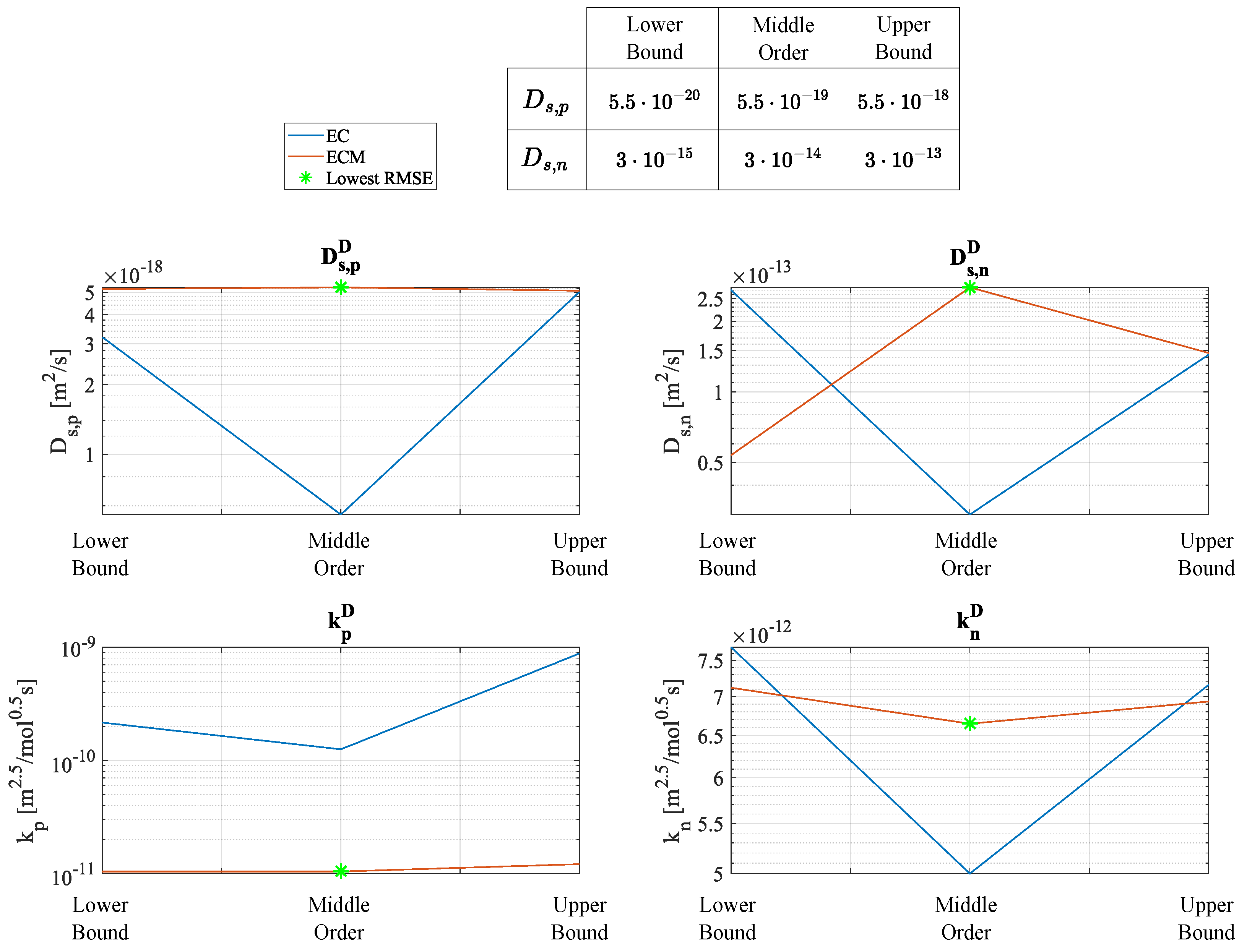
2.5. Error Analysis and Models Comparison

Once the parameters are estimated using the least squares method, the Root Mean Square Errors (RMSEs) of the fitted curves are computed, and the reliability of the parameter estimates is evaluated using the covariance matrix. For n parameters ${\theta }_1,{\theta }_2,\dots ,{\theta }_n$, the covariance matrix $\mathcal{C}$ is expressed, as shown in Equation (20).

$$\mathcal{C}=\left(\begin{array}{cccc}Var\left({\theta }_1\right)& Cov({\theta }_1,{\theta }_2)& \dots & Cov({\theta }_1,{\theta }_n)\\ Cov({\theta }_2,{\theta }_1)& Var\left({\theta }_2\right)& \dots & Cov({\theta }_2,{\theta }_n)\\ ⋮& ⋮& \ddots & ⋮\\ Cov({\theta }_n,{\theta }_1)& Cov({\theta }_n,{\theta }_2)& \dots & Var\left({\theta }_n\right)\end{array}\right)$$

(20)

The diagonal elements $Var\left({\theta }_i\right)$ represent the variances of the individual parameter estimates, indicating the variability in each estimation. The off-diagonal elements $Cov({\theta }_i,{\theta }_j)$ represent the covariance between pairs of parameters, reflecting their linear relationship.

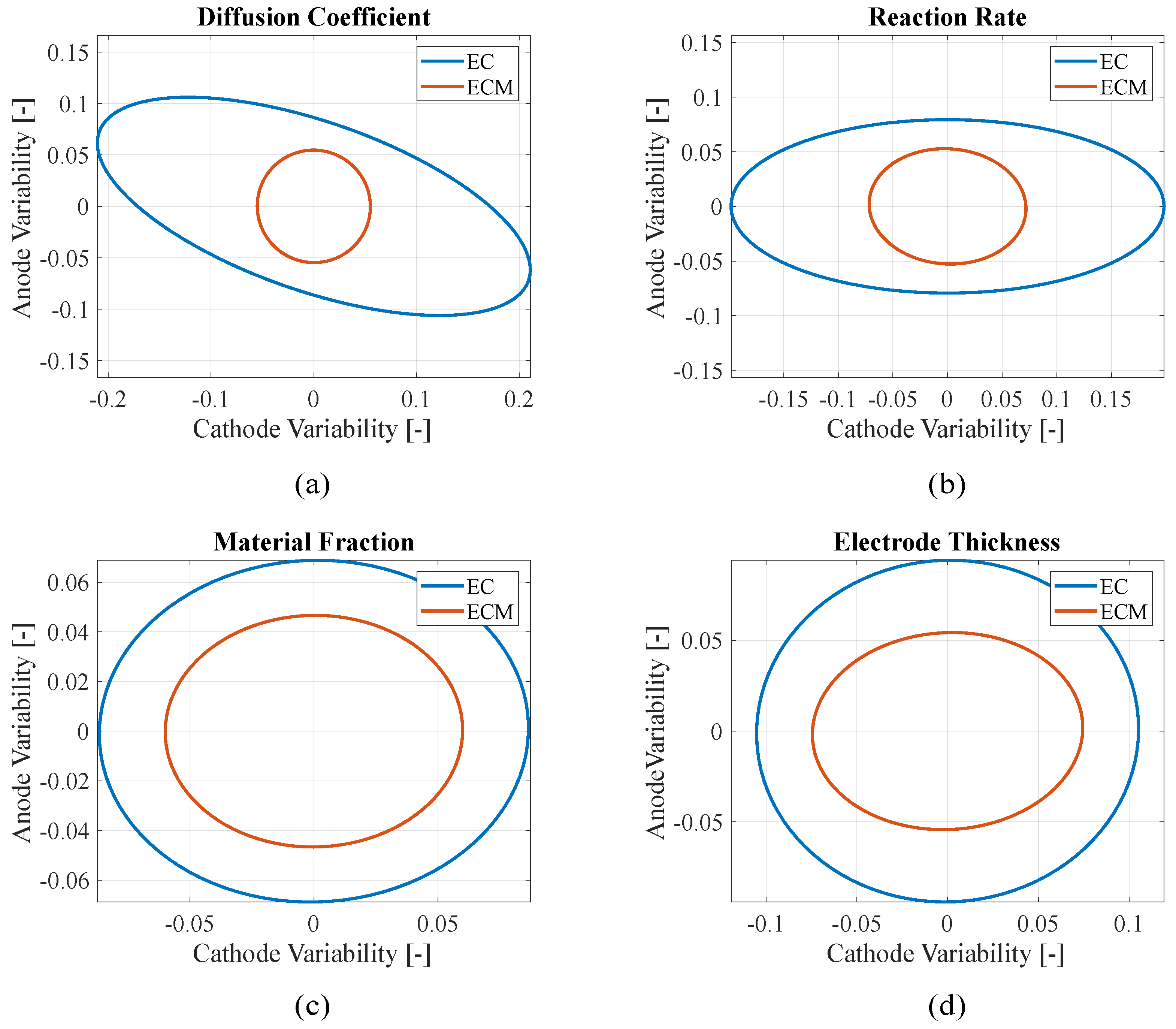
In this model, during the optimization process, each iteration produces a set of parameters that typically improves or maintains the objective function value. These intermediate estimates can be interpreted as a set of plausible solutions within the parameter space. By treating them as empirical samples, it is possible to compute a covariance matrix that captures the spread and correlation of the parameters across iterations. The empirical covariance matrix can then be used to construct confidence (or error) ellipses for selected pairs of parameters. These ellipses are derived from the $2\times 2$ submatrices of the covariance matrix $\mathcal{C}\in {\mathbb{R}}^{nxn}$, which are symmetric and positive definite. The rescaling of the parameters is needed because of the difference in order of magnitude and units of measure of the estimated parameters.

The orientation of the ellipse is determined by the covariance between the two parameters. Specifically, the orientation of the ellipse can be described by an angle $\alpha$, measured with respect to the x-axis: the closer $\alpha$ is to $\pm 45$°, the stronger the correlation between the parameters, while $\alpha =0$° or $\pm 90$° indicates no correlation. On the other hand, a larger ellipse indicates higher variances in the estimated parameters across iterations, suggesting that the algorithm has explored a broader region of the parameter space. While this may reflect a more thorough search of the objective function landscape, it can also be a sign of reduced convergence toward stable parameter values. For this reason, the confidence ellipses—which provide a qualitative representation of the parameter uncertainty and correlation given by the optimization model—should be considered together with the RMSE values to enable a more comprehensive comparison between the electrochemical and the electrochemical–mechanical approach.

3. Experiment

Three commercial LFP/graphite prismatic LIB samples undergo electrical, thermal, and mechanical characterization to evaluate their performance. The tests consist of measuring voltage, temperature, and deformation responses under different charge and discharge currents. Charge rates vary from C/20 to C/2, while discharge rates range from C/20 to 3C, in accordance with manufacturer specifications. Each charge/discharge test is conducted within a state of charge (SOC) range of 0–100% and repeated five times on the same battery sample. A dedicated testing setup with laser sensors is used to monitor battery deformation during operation by measuring thickness variations, as reported in a previous study by the authors [33]. The measured voltage and thickness change, averaged over the tested samples, constitutes the dataset used for parameter estimation through the optimization algorithm.

Differential voltage analysis was performed on a voltage profile recorded during low-rate charge/discharge cycles. Similar results were obtained from charge and discharge measurements. The voltage signal was filtered before computing derivation to mitigate the noise amplification. The Gaussian-weighted moving average filter and the Savitzky–Golay filter were found to be the more effective filtering strategies. The Gaussian filter was applied with the “smoothdata” function in Matlab, activating the option “Gaussian”. Using the window length and a value of 1/20 of the total data points was found to be effective. The Savitzky–Golay filter was applied using the “smooth” function in MATLAB with the “Sgolay” option activated. This filter utilizes the Savitzky–Golay method, which requires specifying both the polynomial degree and the number of data points. It was determined that a third-order polynomial and 1/6 of the total number of data points provided optimal results.

4. Results

4.1. Parameters and Constraints

Certain battery parameters can be measured or evaluated experimentally with relatively simple tests and can therefore be considered known or fixed during the estimation procedure, which helps to reduce the complexity of the simulation. In contrast, some electrochemical parameters—such as diffusion coefficients and reaction rates—require more advanced and complex experimental procedures for accurate identification, and their values reported in the literature often span a wide range. Other physical parameters, such as electrode thickness and the number of electrode layers, can only be determined after battery teardown.

Therefore, alongside the comparison between electrochemical and electrochemical–mechanical parameter estimation, two distinct scenarios were analyzed:

1.

Battery Teardown—The battery has been disassembled, and parameters such as electrode thickness and the number of layers are known. In this case, the set of parameters (${\mathit{\theta }}_{\mathit{td}}$) to be estimated comprises the diffusion coefficients, the reaction rates, and the active material fractions of the two electrodes, as shown in Equation (21):

$${\mathit{\theta }}_{\mathit{td}}=\left\{\begin{array}{cccccc}{D}_{s,p}& D_{s,n}& k_p& k_n& {\zeta }_p& {\zeta }_n\end{array}\right\}$$

(21)

2.

No Battery Teardown—The battery has not been disassembled, and the thickness of the electrodes and the number of layers are unknown. The extended set of parameters (${\mathit{\theta }}_{\mathit{no}-\mathit{td}}$) is presented in Equation (22):

$${\mathit{\theta }}_{\mathit{no}-\mathit{td}}=\left\{\begin{array}{cccc}{\mathit{\theta }}_{\mathbf{td}}& t_p& t_n& N\end{array}\right\}$$

(22)

In this case, it is necessary to constrain the overall battery thickness computed by the model $t_{bat}^{mod}$—accounting for the separator thickness $t_s$, the current collector thickness $t_p^{cc}$, and $t_n^{cc}$ (Equation (23))—to remain within a specified tolerance range around the experimental value $t_{bat}^{exp}$, as shown in Equation (24).

$$t_{bat}^{mod}=N(t_p+t_s+t_n)+{\displaystyle \frac{N}{2}}(t_p^{cc}+t_n^{cc})+2t_{case}$$

(23)

$${\displaystyle \frac{|t_{bat}^{mod}-t_{bat}^{exp}|}{t_{bat}^{exp}}}\le to{l}_{thick}$$

(24)

Then, the parameters sets ${\mathit{\theta }}_{\mathbf{td}}$ and ${\mathit{\theta }}_{\mathit{no}-\mathit{td}}$ are estimated by fitting experimental curves obtained from constant current cycles with a 100% depth of discharge (DOD) at a $C/2$ current rate. In both scenarios, the stoichiometric windows are calculated with differential voltage analysis (DVA) at low current rates. The stoichiometric indexes corresponding to $SOC=100\%$ ($x_{100}$ and $y_{100}$) are imposed as fixed initial values during discharge, while $x_0$ and $y_0$ are constrained around their corresponding experimental value with a certain tolerance ($to{l}_{x_0}$ and $to{l}_{y_0}$ respectively), as shown in Equation (25).

$${\displaystyle \frac{|x_0^{mod}-x_0^{exp}|}{x_o^{exp}}}\le to{l}_{x_0}{\displaystyle \frac{|y_0^{mod}-y_0^{exp}|}{y_o^{exp}}}\le to{l}_{y_0}$$

(25)

However, the estimation cannot be considered complete: the diffusion coefficients are current-dependent [23], and the contact resistance $R_c$—which is another challenging parameter to assess—is voltage-insensitive at low current rates, namely, its value does not influence the voltage when the current is low. Therefore, the experimental data at $3C$ discharge current rate are then used to assess $R_c$ and extrapolate the diffusion coefficient behavior $D_{s,k}\left(i\right)$ by linearly fitting the estimated $D_{s,k}\left(i_{C/2}\right)$ and $D_{s,k}\left(i_{3C}\right)$.

Among the other parameters—considered fixed in the optimization process—there are material properties, like the molar mass $M_m$ and the crystal density ${\rho }^{crystal}$ of the active materials’ lattice structure; the corresponding maximum lithium concentration that can be obtained, as stated in Equation (3); electrolyte properties; solid-phase conductivity; and the active material particle radius. Electrolyte parameters have a minor influence on the results; thus, they are taken from the literature. The influence of the active material particle radius on the results is correlated with the diffusion coefficient, making the estimation of both parameters trivial. The fixed parameters are reported in

Table 2. Fixed parameters: l, from the literature; c, calculated; m, measured.

Parameter	Symbol	Cathode	Separator	Anode	Unit
Molar mass	Mmk	157.76 c	−	79 c	g/mol
Crystal density	${\rho }_k^{crystal}$	3600 l	−	2260 l	kg/m3
Maximum concentration	$c_{s,k}^{max}$	22,820 c	−	28,600 c	mol/m3
Electrolyte diffusivity	$D_{e,k}$	$1.3·{10}^{-10}$l [34]	$1.3·{10}^{-10}$l [34]	$1.3·{10}^{-10}$l [34]	m2/s
Solid-phase conductivity	${\sigma }_{s,k}$	6 l [23]	−	100 l [35]	S/m
Transference number	$t_{+}$		$0.363$l [23]		−
Bruggeman coefficient	$brugg$		$1.5$l [36]		−
Particle radius	$R_k$	$0.03$m	−	10 m	$\mathsf{\mu }$m

.

4.2. Teardown Configuration

In this configuration, the electrode thickness and the number of layers are known via SEM analysis conducted after battery teardown, as illustrated in Figure 3 [16]. The estimation procedure requires initial guess values as a starting point for the parameters to be estimated. The initial value of the active material fraction can be evaluated from the electrode capacity at low discharge rates—in which the stoichiometric window is known—from the relation expressed in Equation (26). On the other hand, the diffusion coefficients and reaction rates are selected based on values commonly reported in the literature, which often span several orders of magnitude. In particular, Delacourt et al. [37] and Northrop et al. [34] reported representative values for the diffusion coefficients of LFP and graphite, respectively, while Maheshwari et al. [23] provided a comprehensive review of the ranges of reaction rate constants for both electrodes. The parameter ranges were taken from these references, and the initial guesses were chosen from the central order of magnitude of these ranges, as presented in

Table 3. Teardown scenario—parameters bound and comparison between the electrochemical (EC) and electrochemical–mechanical (ECM) estimate.

Current Rate	Symbol	Initial Value	Lower Bound	Upper Bound	EC Estimate	ECM Estimate	Unit
$C/2$	$D_{s,p}$	$5.5·{10}^{-19}$	$5.5·{10}^{-20}$	$5.5·{10}^{-18}$	$5.5·{10}^{-19}$	$5.25·{10}^{-18}$	m2/s
	$D_{s,n}$	$3·{10}^{-14}$	$3·{10}^{-15}$	$3·{10}^{-13}$	$3·{10}^{-14}$	$2.79·{10}^{-13}$	m2/s
	$k_p$	$1·{10}^{-10}$	$1·{10}^{-11}$	$1·{10}^{-9}$	$1.2·{10}^{-10}$	$1·{10}^{-11}$	m2.5/mol0.5s
	$k_n$	$5·{10}^{-12}$	$5·{10}^{-13}$	$5·{10}^{-11}$	$5·{10}^{-12}$	$6.65·{10}^{-12}$	m2.5/mol0.5s
	${\zeta }_p$	$0.398$	$0.2$	$0.6$	$0.398$	$0.402$	−
	${\zeta }_n$	$0.53$	$0.3$	$0.7$	$0.531$	$0.532$	−
$3C$	$D_{s,p}$	$5.5·{10}^{-19}$	$5.5·{10}^{-20}$	$5.5·{10}^{-18}$	$5.57·{10}^{-19}$	$5.25·{10}^{-18}$	m2/s
	$D_{s,n}$	$3·{10}^{-14}$	$3·{10}^{-15}$	$3·{10}^{-13}$	$3.44·{10}^{-14}$	$1.4·{10}^{-13}$	m2/s
	$R_c$	$0.002$	$0.001$	$0.1$	$0.0016$	$0.0025$	$\Omega$m2

, together with the final estimated values. Then, an additional analysis was performed by varying the initial values to assess the impact on the estimation results, as described in Section 4.5.

$$C_p={\displaystyle \frac{c_{s,p}^{max}\Delta yFNA{t}_p{\zeta }_p}{3600}}{C}_n={\displaystyle \frac{c_{s,n}^{max}\Delta xFNA{t}_n{\zeta }_n}{3600}}$$

(26)

Figure 4 shows the voltage profile and the thickness change obtained at the end of the optimization process with the two estimation approaches in the teardown scenario. Furthermore,

Table 4. Teardown scenario−RMSEs of the voltage profile, thickness change, and capacity.

Property	RMSE-EC	RMSE-ECM	Unit
Voltage	0.0692	0.0052	V
Thickness change	0.0258	0.0091	mm
Capacity	3.92	0.174	Ah

shows the corresponding Root Mean Square Errors (RMSEs) as a sum of the RMSEs computed at $C/2$ and at $3C$: the electrochemical–mechanical (ECM) approach leads to more accurate prediction of the battery behavior, presenting significantly lower errors; in fact, the electrochemical (EC) approach converges faster due to the simplicity of the objective function but leads to less accurate estimate. In addition, Figure 5 presents the confidence ellipses of paired parameters to compare the stability of the two approaches: adding the mechanical constraints makes the algorithm more reliable, reducing parameter variability with respect to just using electrochemical objective functions. In fact, smaller ellipses indicate that the parameters present lower variance throughout the iterations, which is a sign of improved convergence toward the final value. However, small ellipses may also result from the algorithm rapidly converging to a local minimum of the objective function without exploring a wide range of the possible parameters. For this reason, the confidence ellipses should be interpreted alongside the RMSEs to better assess the overall quality and reliability of the model. In this case, the electrochemical-only approach leads both to higher RMSEs and larger ellipses with respect to the electrochemical–mechanical approach, making parameter identification with the latter approach more reliable.

4.3. No Teardown Configuration

In this configuration, even the electrode thickness and the number of layers must be estimated. While this increases the computational complexity, it also enables the estimation of such parameters without the need for battery teardown. To assess the robustness of the model, the initial values for the electrode thickness were deliberately set slightly different from the measured ones. However, as shown in

Table 5. No teardown scenario—parameters bound and comparison between the electrochemical (EC) and electrochemical–mechanical (ECM) estimate.

Current Rate	Symbol	Initial Value	Lower Bound	Upper Bound	EC Estimate	ECM Estimate	Unit
$C/2$	$D_{s,p}$	$5.5·{10}^{-19}$	$5.5·{10}^{-20}$	$5.5·{10}^{-18}$	$5.52·{10}^{-19}$	$4.72·{10}^{-19}$	m2/s
	$D_{s,n}$	$3·{10}^{-14}$	$3·{10}^{-15}$	$3·{10}^{-13}$	$3.55·{10}^{-14}$	$3.54·{10}^{-14}$	m2/s
	$k_p$	$1·{10}^{-10}$	$1·{10}^{-11}$	$1·{10}^{-9}$	$1.26·{10}^{-10}$	$7.83·{10}^{-10}$	m2.5/mol0.5s
	$k_n$	$5·{10}^{-12}$	$5·{10}^{-13}$	$5·{10}^{-11}$	$5.39·{10}^{-12}$	$6.81·{10}^{-12}$	m2.5/mol0.5s
	${\zeta }_p$	$0.398$	$0.2$	$0.6$	$0.397$	$0.395$	−
	${\zeta }_n$	$0.53$	$0.3$	$0.7$	$0.532$	$0.521$	−
	$t_p$	67	50	100	$71.8$	$72.5$	$\mathsf{\mu }$m
	$t_n$	57	50	100	$60.5$	61	$\mathsf{\mu }$m
	N	140	135	145	143	143	−
$3C$	$D_{s,p}$	$5.5·{10}^{-19}$	$5.5·{10}^{-20}$	$5.5·{10}^{-18}$	$8.23·{10}^{-19}$	$5.71·{10}^{-19}$	m2/s
	$D_{s,n}$	$3·{10}^{-14}$	$3·{10}^{-15}$	$3·{10}^{-13}$	$1·{10}^{-13}$	$7.37·{10}^{-14}$	m2/s
	$R_c$	$0.002$	$0.001$	$0.1$	$0.0024$	$0.0023$	$\Omega$m2

, the end values of these parameters’ results are close to the one imposed in the teardown condition.

Figure 6 shows the voltage profile and the thickness change obtained at the end of the optimization process, while

Table 6. No teardown scenario—RMSEs of the voltage profile, thickness change, and capacity.

Property	RMSE-EC	RMSE-ECM	Unit
Voltage	0.057	0.063	V
Thickness change	0.0126	0.0120	mm
Capacity	0.65	0.84	Ah

reports the corresponding RMSEs in the configuration without battery teardown. In this scenario, the difference between the two models is negligible both in the estimation and therefore in the committed error: adding new capacity-sensitive parameters to be estimated avoids the wrong convergence reached in the previous scenario with the electrochemical-only approach. However, in this case, the main difference between the two models is in their capability of generating reliable solutions. In fact, even in this scenario, the electrochemical–mechanical approach is able to increase the reliability of the estimation, as presented in Figure 7, comparing the area of the confidence ellipses between the two models.

4.4. Validation

The obtained parameters were then used to validate the reliability of the estimation, computing the model at different discharge current rates and comparing the results with the experimental values. Figure 8 and Figure 9 present the teardown scenario with the electrochemical and electrochemical–mechanical estimated parameters, respectively. In the teardown scenario, as shown in Section 4.2, the electrochemical-only approach converged to less accurate parameters, resulting in a less accurate prediction of the battery behavior at different current rates. Conversely, with the same initial conditions, the electrochemical–mechanical approach reaches better results. In the no-teardown scenario (Figure 10 and Figure 11), there is no significant difference in the battery behavior between the two estimation models because the number of the capacity sensitive parameters increased. The advantage of using the electrochemical–mechanical approach is in the reliability of its estimates.

4.5. Sensitivity to Initial Guesses

Finally, to assess the stability of the model, the parameter estimation was repeated using different initial values, specifically the lower and upper bounds of the considered ranges. Focusing on the teardown scenario, the analysis was performed on the diffusion coefficients, as these parameters span several orders of magnitude. The effect on the estimation of the parameters was examined: no significant difference was observed in the estimation of the active material fractions, while the variations in the diffusion coefficients themselves and reaction rates are reported in Figure 12. Given the non-convex nature of the objective function—namely, the presence of multiple local minima—there is no unique set of parameters to which the algorithm will necessarily converge. Nevertheless, the electrochemical–mechanical approach exhibits greater stability, tending to converge to similar values even when different initial guesses are used. In fact, the inclusion of mechanical measurements provides further information and constraints that reduce the sensitivity to initial parameter guesses, thereby lowering the risk of the algorithm converging to a local minimum that is less representative of the actual cell response.

5. Conclusions

In this study, a parameter estimation framework was developed by integrating both electrochemical and mechanical measurements into the parameter estimation process. The inclusion of mechanical data, such as the battery thickness change, introduces additional constraints that significantly enhance the identifiability of key parameters, particularly those related to diffusion and reaction kinetics.

Two scenarios were considered: one where the battery underwent teardown to measure electrode thicknesses and the number of layers, and one without teardown. In the first case, the electrochemical-only estimation, constrained by fewer free parameters, converged to incorrect solutions, while the electrochemical–mechanical approach reached satisfying estimates with lower RMSEs and parameter variability. In the second case, where no teardown was performed and a greater number of parameters remain uncertain and must be identified, the results obtained with both electrochemical and electrochemical–mechanical approaches are comparable but the first showed higher uncertainty.

In conclusion, integrating mechanical data consistently improves accuracy and robustness of the estimation, reducing parameter variability and sensitivity to initial guesses.

References

1. Degen, F. Lithium-ion battery cell production in Europe: Scenarios for reducing energy consumption and greenhouse gas emissions until 2030. J. Ind. Ecol. 2023, 27, 964–976. [Google Scholar] [CrossRef]
2. Yang, Y.; Okonkwo, E.G.; Huang, G.; Xu, S.; Sun, W.; He, Y. On the sustainability of lithium ion battery industry—A review and perspective. Energy Storage Mater. 2021, 36, 186–212. [Google Scholar] [CrossRef]
3. Tran, M.K.; Mathew, M.; Janhunen, S.; Panchal, S.; Raahemifar, K.; Fraser, R.; Fowler, M. A comprehensive equivalent circuit model for lithium-ion batteries, incorporating the effects of state of health, state of charge, and temperature on model parameters. J. Energy Storage 2021, 43, 103252. [Google Scholar] [CrossRef]
4. Lagnoni, M.; Scarpelli, C.; Lutzemberger, G.; Bertei, A. Critical comparison of equivalent circuit and physics-based models for lithium-ion batteries: A graphite/lithium-iron-phosphate case study. J. Energy Storage 2024, 94, 112326. [Google Scholar] [CrossRef]
5. Ali, H.A.A.; Raijmakers, L.H.; Chayambuka, K.; Danilov, D.L.; Notten, P.H.; Eichel, R.A. A comparison between physics-based Li-ion battery models. Electrochim. Acta 2024, 493, 144360. [Google Scholar] [CrossRef]
6. Doyle, M.; Fuller, T.F.; Newman, J. Modeling of galvanostatic charge and discharge of the lithium/polymer/insertion cell. J. Electrochem. Soc. 1993, 140, 1526. [Google Scholar] [CrossRef]
7. Valøen, L.O.; Reimers, J.N. Transport Properties of LiPF6-Based Li-Ion Battery Electrolytes. J. Electrochem. Soc. 2005, 152, A882. [Google Scholar] [CrossRef]
8. Bergstrom, H.K.; Fong, K.D.; McCloskey, B.D. Interfacial Effects on Transport Coefficient Measurements in Li-ion Battery Electrolytes. J. Electrochem. Soc. 2021, 168, 060543. [Google Scholar] [CrossRef]
9. Khalik, Z.; Donkers, M.; Sturm, J.; Bergveld, H. Parameter estimation of the Doyle–Fuller–Newman model for Lithium-ion batteries by parameter normalization, grouping, and sensitivity analysis. J. Power Sources 2021, 499, 229901. [Google Scholar] [CrossRef]
10. Jin, N.; Danilov, D.; Hof, P.; Donkers, M. Parameter estimation of an electrochemistry-based lithium-ion battery model using a two-step procedure and a parameter sensitivity analysis. Int. J. Energy Res. 2018, 42, 2417–2430. [Google Scholar] [CrossRef]
11. Marcicki, J.; Canova, M.; Conlisk, A.T.; Rizzoni, G. Design and parametrization analysis of a reduced-order electrochemical model of graphite/LiFePO4 cells for SOC/SOH estimation. J. Power Sources 2013, 237, 310–324. [Google Scholar] [CrossRef]
12. Miguel, E.; Plett, G.L.; Trimboli, M.S.; Oca, L.; Iraola, U.; Bekaert, E. Review of computational parameter estimation methods for electrochemical models. J. Energy Storage 2021, 44, 103388. [Google Scholar] [CrossRef]
13. Ha, S.; Onori, S. COBRAPRO: A MATLAB toolbox for Physics-based Battery Modeling and Co-simulation Parameter Optimization. arXiv 2024, arXiv:2404.10022. [Google Scholar] [CrossRef]
14. Planden, B.; Courtier, N.E.; Robinson, M.; Khetarpal, A.; Planella, F.B.; Howey, D.A. PyBOP: A Python package for battery model optimisation and parameterisation. arXiv 2024, arXiv:2412.15859. [Google Scholar]
15. Zhang, L.; Wang, L.; Hinds, G.; Lyu, C.; Zheng, J.; Li, J. Multi-objective optimization of lithium-ion battery model using genetic algorithm approach. J. Power Sources 2014, 270, 367–378. [Google Scholar] [CrossRef]
16. Clerici, D.; Mocera, F.; Soma, A. Electrochemical–mechanical multi-scale model and validation with thickness change measurements in prismatic lithium-ion batteries. J. Power Sources 2022, 542, 231735. [Google Scholar] [CrossRef]
17. Mohtat, P.; Lee, S.; Sulzer, V.; Siegel, J.B.; Stefanopoulou, A.G. Differential Expansion and Voltage Model for Li-ion Batteries at Practical Charging Rates. J. Electrochem. Soc. 2020, 167, 110561. [Google Scholar] [CrossRef]
18. Rieger, B.; Schlueter, S.; Erhard, S.V.; Schmalz, J.; Reinhart, G.; Jossen, A. Multi-scale investigation of thickness changes in a commercial pouch type lithium-ion battery. J. Energy Storage 2016, 6, 213–221. [Google Scholar] [CrossRef]
19. Sauerteig, D.; Hanselmann, N.; Arzberger, A.; Reinshagen, H.; Ivanov, S.; Bund, A. Electrochemical-mechanical coupled modeling and parameterization of swelling and ionic transport in lithium-ion batteries. J. Power Sources 2018, 378, 235–247. [Google Scholar] [CrossRef]
20. Clerici, D.; Pistorio, F.; Scalzo, S.; Martelli, S.; Mocera, F.; Somà, A. Mechanical Multiscale Lithium-Ion Battery Modeling for Optimized Battery Pack Design. Eng. Proc. 2025, 85, 48. [Google Scholar] [CrossRef]
21. Powell, M.J.D. The BOBYQA Algorithm for Bound Constrained Optimization Without Derivatives; Technical Report NA2009/06; Department of Applied Mathematics and Theoretical Physics, University of Cambridge: Cambridge, UK, 2009. [Google Scholar]
22. Sun, W.; Li, Q.; Xiao, P.; Carbone, P. Determination of the tortuosity of a Li-ion battery separator. J. Energy Storage 2024, 97, 112940. [Google Scholar] [CrossRef]
23. Maheshwari, A.; Dumitrescu, M.A.; Destro, M.; Santarelli, M. Inverse parameter determination in the development of an optimized lithium iron phosphate – Graphite battery discharge model. J. Power Sources 2016, 307, 160–172. [Google Scholar] [CrossRef]
24. Wang, A.A.; O’Kane, S.E.J.; Brosa Planella, F.; Houx, J.L.; O’Regan, K.; Zyskin, M.; Edge, J.; Monroe, C.W.; Cooper, S.J.; Howey, D.A.; et al. Review of parameterisation and a novel database (LiionDB) for continuum Li-ion battery models. Prog. Energy 2022, 4, 032004. [Google Scholar] [CrossRef]
25. Didier, C.; Pang, W.K.; Guo, Z.; Schmid, S.; Peterson, V.K. Phase Evolution and Intermittent Disorder in Electrochemically Lithiated Graphite Determined Using in Operando Neutron Diffraction. Chem. Mater. 2020, 32, 2518–2531. [Google Scholar] [CrossRef]
26. Padhi, A.K.; Nanjundaswamy, K.S.; Goodenough, J.B. Phospho-olivines as positive-electrode materials for rechargeable lithium batteries. J. Electrochem. Soc. 1997, 144, 1188. [Google Scholar] [CrossRef]
27. Schweidler, S.; de Biasi, L.; Schiele, A.; Hartmann, P.; Brezesinski, T.; Janek, J. Volume changes of graphite anodes revisited: a combined operando X-ray diffraction and in situ pressure analysis study. J. Phys. Chem. C 2018, 122, 8829–8835. [Google Scholar] [CrossRef]
28. Gomadam, P.M.; Weidner, J.W. Modeling volume changes in porous electrodes. J. Electrochem. Soc. 2005, 153, A179. [Google Scholar] [CrossRef]
29. Clerici, D. Mechanics of Lithium-Ion Batteries—A Modelling and Experimental Perspective. Ph.D. Thesis, Department of Mechanical and Aerospace Engineering, Politecnico di Torino, Italy, 2024. [Google Scholar]
30. Clerici, D.; Pistorio, F.; Mocera, F.; Somà, A. Mechanical characterization and modelling of lithium-ion batteries. Transp. Res. Procedia 2023, 70, 276–283. [Google Scholar] [CrossRef]
31. Zitzler, E.; Thiele, L. Multiobjective evolutionary algorithms: a comparative case study and the strength Pareto approach. IEEE Trans. Evol. Comput. 1999, 3, 257–271. [Google Scholar] [CrossRef]
32. Zitzler, E.; Deb, K.; Thiele, L. Comparison of Multiobjective Evolutionary Algorithms: Empirical Results. Evol. Comput. 2000, 8, 173–195. [Google Scholar] [CrossRef]
33. Clerici, D.; Martelli, S.; Mocera, F.; Somà, A. Mechanical characterization of lithium-ion batteries with different chemistries and formats. J. Energy Storage 2024, 84, 110899. [Google Scholar] [CrossRef]
34. Northrop, P.W.C.; Ramadesigan, V.; De, S.; Subramanian, V.R. Coordinate Transformation, Orthogonal Collocation, Model Reformulation and Simulation of Electrochemical-Thermal Behavior of Lithium-Ion Battery Stacks. J. Electrochem. Soc. 2011, 158, A1461–A1477. [Google Scholar] [CrossRef]
35. Christensen, J. Modeling Diffusion-Induced Stress in Li-Ion Cells with Porous Electrodes. J. Electrochem. Soc. 2010, 157, A366. [Google Scholar] [CrossRef]
36. Doyle, M.; Fuentes, Y. Computer Simulations of a Lithium-Ion Polymer Battery and Implications for Higher Capacity Next-Generation Battery Designs. J. Electrochem. Soc. 2003, 150, A706. [Google Scholar] [CrossRef]
37. Delacourt, C.; Safari, M. Analysis of lithium deinsertion/insertion in LiyFePO4 with a simple mathematical model. Electrochimica Acta 2011, 56, 5222–5229. [Google Scholar] [CrossRef]
Figure 1. Crystal lattice strain of (a) LFP and (b) graphite as a function of lithium content expressed with the state of lithiation of the electrode.
Applsci 15 07217 g001
Figure 2. Electrochemical–mechanical model framework: from the lithium concentration obtained from P2D model to particle deformation at different positions along the direction of electrode’s width (z). The superscript c and a indicate cathode and anode, while l and p indicate lattice and particle, respectively. n and m denote the number of discretization points.
Applsci 15 07217 g002
Figure 3. SEM analysis of graphite-LFP battery samples. (a) Graphite electrode, (b,c) graphite and LFP electrodes, and separator and current collector.
Applsci 15 07217 g003
Figure 4. Teardown scenario−a comparison of (a) voltage profile and (b) thickness change between the experimental data and the model computed with the estimated electrochemical (EC) and electrochemical−mechanical (ECM) parameters.
Applsci 15 07217 g004
Figure 5. Teardown scenario−comparison between electrochemical (EC) and electrochemical−mechanical (ECM) estimation variability of (a) diffusion coefficients, (b) reaction rates, and (c) material fractions of the electrodes.
Applsci 15 07217 g005
Figure 6. Teardown scenario−comparison of (a) voltage profile and (b) thickness change between the experimental data and the model computed with the estimated electrochemical (EC) and electrochemical−mechanical (ECM) parameters.
Applsci 15 07217 g006
Figure 7. No teardown scenario−comparison between electrochemical (EC) and electrochemical–mechanical (ECM) estimation variability of (a) diffusion coefficients, (b) reaction rates, (c) material fractions, and (d) thickness of the electrodes.
Applsci 15 07217 g007
Figure 8. Teardown scenario−comparison of (a) voltage profile and (b) thickness change between the experimental data and the model computed with the electrochemical (EC) estimated parameters.
Applsci 15 07217 g008
Figure 9. Teardown scenario−comparison of (a) voltage profile and (b) thickness change between the experimental data and the model computed with the estimated electrochemical−mechanical (ECM) parameters.
Applsci 15 07217 g009
Figure 10. No teardown scenario−comparison of (a) voltage profile and (b) thickness change between the experimental data and the model computed with the estimated electrochemical (EC) parameters.
Applsci 15 07217 g010
Figure 11. No teardown scenario−comparison of (a) voltage profile and (b) thickness change between the experimental data and the model computed with the estimated electrochemical−mechanical (ECM) parameters.
Applsci 15 07217 g011
Figure 12. Variation in the estimated values of the diffusion coefficients and reaction rates when using different initial guesses of diffusion coefficients. The green asterisk indicates the best parameter set, corresponding to the lowest RMSE.
Applsci 15 07217 g012