Data Leveling of Multi-Map Geochemical Exploration Data Using Compositional Data Analysis: A Case Study from the Baiyinchagan–Maodeng Area, Inner Mongolia, China

Abstract

Exploration geochemical data are typically collected and analyzed according to standard map sheets. Different map sheets may be tested by different companies, at different times, or using different instruments. As a result, “systematic errors” inevitably arise, which are directly reflected in the “shift” effect between different map sheets. This study compares various leveling methods, including contrast return (CR), boundary leveling (BL), and multi-scale correction (MSC), based on compositional data transformation of six map sheets from the Baiyinchagan–Maodeng area. The results show the following features: the raw data from multiple map sheets contain certain errors, and these raw data cannot be directly used to create geochemical maps; the CR method is unsuitable for leveling in areas with small scales or significant geological background differences; the BL method yields more reasonable results when there is a similar geochemical background (geological background) between map sheets, and it is better suited for leveling between map sheets in areas with small scales or significant regional differences in geochemical backgrounds; finally, the MSC method yields results similar to the BL method, but it does not require boundary consistency, thus having fewer limitations, although it requires multi-scale geochemical data. In practical terms, this study provides valuable guidance for selecting appropriate geochemical data leveling methods in exploration projects, thereby improving the accuracy and reliability of geochemical mapping and enhancing the effectiveness of mineral exploration.

1. Introduction

For regional mineral exploration, geochemical exploration is an intuitive and effective approach. In China, between 1981 and 2005, the Ministry of Geology and the Ministry of Land and Resources, based on the “The Regional Geochemistry National Reconnaissance (RGNR)”, identified 58,788 anomalies across the country. These anomalies led to the discovery of 3349 mineral deposits, playing a significant role in the discovery of mineral deposits in China [1,2,3,4]. Geochemical exploration for mineral prospecting requires the study area to be divided into standard sizes of different scales, such as 1:250,000, 1:200,000, and 1:50,000 [5]. The work between these different map sheets may be carried out by different companies, at different times, and in different laboratories, which inevitably leads to “shift” effects due to systematic errors. This not only affects the visual appeal of the map sheets but also introduces errors in the judgment on the background areas and prediction of target areas [6,7].

To address the “shift” effect of geochemical exploration data between different map sheets, many researchers have proposed various leveling methods suitable for different situations. For example, Daneshfar and Cameron [6] proposed a method to calculate the linear relationship between two survey areas using percentiles, and tested it on Mo elements in stream sediments. Williams [8] proposed a data leveling method based on compositional data analysis. Pereira [7] also applied linear regression equations to perform leveling of the element Ni in soil in the Wallonia region. Additionally, Wang et al. [9] compared the effectiveness of several common leveling methods, including adjustment methods, normalization methods, least squares methods, and median transformation methods. However, these existing methods exhibit varying degrees of limitations. For instance, methods relying on linear regression or percentiles may not adequately account for the inherent compositional nature of geochemical data, where elements are interrelated and subject to the closure effect. Similarly, normalization or median transformation methods might obscure subtle geochemical anomalies, especially in areas with highly heterogeneous geological backgrounds where element distributions can vary significantly even within a single map sheet. A critical comparison reveals that no single method is universally optimal; their effectiveness often depends heavily on the specific characteristics of the dataset, such as the strength of compositional effects and the degree of geological heterogeneity.

The purpose of these data processing methods is to eliminate the shift effect at map sheet boundaries. However, there are several important points to note: First, the leveling process is generally based on statistical principles, so the data should roughly follow a normal distribution before processing. Second, the leveled data still belong to compositional data, which inherently contains the “closure effect”. This may lead to pseudo-correlation between geochemical elements, causing the data analysis results to become unstable. Third, most of the leveling methods perform calibration on the entire map sheet as a unit. However, if there are significant geochemical background differences between map sheets, this method may not be applicable.

Therefore, in this study we processed the raw data through compositional data transformation, which could account for the inter-element relationships where the increase or decrease in one element’s concentration might be related to changes in others, thereby eliminating the skewed distribution and closure effects inherent in such data. Then, we compared the leveling effects of the contrast return method (CR), boundary leveling method (BL), and multi-scale correction method (MSC), selecting the most suitable leveling method to provide reference for future processing of similar areas or data.

2. Geological Overview

2.1. Regional Geological Background

The southern section of the Greater Khingan Range is located within the Xing–Mong orogenic belt in the eastern part of the Central Asian Orogenic Belt (Figure 1). It is one of the most important tin–copper–silver polymetallic metallogenic belts in northern China [10]. Before the Mesozoic, the study area was part of the continental margin of the North China Plate on the southern side of the Central Asian–Mongolian Ocean.

After the Mesozoic, the study area was influenced by both the tectonics formed before and during the closure of the Central Asian–Mongolian Ocean, and by the tectonic domain of the Pacific Rim. This led to the transformation of these east–west trending faults into shear transformation faults. It is in these regions, where tectonic fields from different eras and directions intersect and overlap, that a unique and highly favorable tectonic dynamic background was formed. The intricate distribution of faults plays a decisive role in the tectonics and mineralization of the southern section of the Greater Khingan Range [11].

2.2. Geological Features of the Study Area

The Paleozoic strata of the study area belong to the Xilamulun Stratigraphic Zone, with the northern part extending into the Zhongdong Ujumqin Stratigraphic Subzone of the Inner Mongolia–Xing’an Stratigraphic Zone. The lower Paleozoic is poorly developed, being eroded by plutons and covered by Mesozoic strata, with only sporadic exposures. The Carboniferous–Permian strata are well developed and are the main ore-bearing strata, where the primary ore deposit type is magmatic hydrothermal. The Mesozoic strata belong to the Inner Mongolia–Songliao Stratigraphic Zone, specifically the Zhonglian Stratigraphic Subzone, where the Cretaceous is the most developed and widespread throughout the region. The Paleogene–Neogene strata are located in the Inner Mongolia Stratigraphic Zone, in the Xilingol Stratigraphic Subzone, mainly consisting of the Neogene Baogeda Ula Formation. The Quaternary is the most widely distributed, located in the Northeast Stratigraphic Region, Inner Mongolia Stratigraphic Zone, Erin–Genghe Stratigraphic Subzone (Figure 2).

The main tectonic features of the study area are folds and faults. The folds are primarily composite folds—oriented NE or NEE, formed during the Late Hercynian orogeny. The faults mainly result from the NW–SE compressional folding of the strata during the Late Hercynian, creating reverse faults predominantly oriented NE–NEE. During the subsequent Yanshan period, the NE-oriented faults from the Late Hercynian were inherited and further developed [12,13].

Throughout the long geological history, regional tectonic movements have led to frequent and intense magmatic activity in the area. The intrusive rocks are characterized by multiple phases, types, and widespread distribution, extending from the northeast to the southwest across the study area. From the Late Paleozoic to the Mesozoic, intrusive rocks of mafic, intermediate, and felsic compositions have developed, generally exhibiting NE to nearly E–W orientations.

Late Paleozoic intrusions are mainly distributed in the southwest and northeast of the study area, while Mesozoic intrusions are found in the central and eastern parts of the area. In terms of magmatic activity periods, the intrusive rocks in the study area experienced three tectonic–magmatic phases: the Hercynian, Indosinian, and Yanshan periods (Figure 2). The Hercynian intrusive rocks mainly include Middle Devonian quartz diorite, Late Devonian granite diorite, and diorite; Early Carboniferous granite diorite, biotite granite, Late Carboniferous pyroxenite, diorite, hornblende diorite, diorite, granite diorite, and biotite granite; Early Permian hornblende diorite, biotite granite, and Middle Permian diorite, hornblende diorite, diorite, and quartz monzonite. The Indosinian intrusive rocks mainly include Middle Triassic medium-grained porphyritic biotite granite, Middle Triassic fine-grained porphyritic biotite granite, and Late Triassic fine-grained biotite granite. The Yanshan intrusive rocks mainly include Early Cretaceous fine-grained porphyritic granite and medium-grained porphyritic granite [10].

3. Data Introduction

The study area contains geochemical data at 1:50,000 and 1:200,000 scales, which are introduced separately below.

3.1. The 1:50,000 Scale Data Source and Analytical Methods

Since the samples were collected by two different organizations, for ease of subsequent description, the study area is divided into northern and southern regions. The 1:50,000 scale soil geochemical data for the northern area, including L50E021011, L50E022011, and L50E022012, were completed by the Geological Survey Institute of China University of Geosciences (Beijing) from 2009 to 2013, with a total of 3826 data points. The southern area, including L50E023011, L50E023012, and L50E024011, was completed by the Tianjin Geological Survey Research Center from 2010 to 2013, with a total of 6924 data points. The soil geochemical survey was conducted in accordance with the “Geochemical Survey Specifications” (1:50,000 scale), with a sampling density of 8–20 points/km². The sampling targets were residual slope deposits close to the bedrock surface (Figure 3a).

A total of 12 elements were analyzed in the samples. Pb, Mo, Sn, Cu, Ag, Zn, Ni, and Co elements across all map sheets were analyzed using electrode spectroscopy (ES); As, Sb, and Bi elements were analyzed using atomic fluorescence spectroscopy (AFS); and W was analyzed using the polarographic method (POL) (

Table 1. The elements, analytical methods, and detection limits of the 1:50,000 scale data.

Element	Unit	Detection Limit	Analysis Method
Pb	μg/g	0.5	ES
Mo	μg/g	0.2	ES
Sn	μg/g	0.2	ES
Cu	μg/g	0.5	ES
Ag	μg/g	0.02	ES
Zn	μg/g	11.2	ES
Ni	μg/g	0.8	ES
Co	μg/g	0.8	ES
As	μg/g	0.2	AFS
Sb	μg/g	0.05	AFS
Bi	μg/g	0.05	AFS
W	μg/g	0.25	POL

Note: ES: electrode spectroscopy; AFS: atomic fluorescence spectroscopy; POL: polarography; μg/g: micrograms per gram.

). All geochemical sample testing and analysis were completed by the Inner Mongolia Land and Resources Exploration and Development Institute Laboratory, with an internal inspection pass rate for all samples greater than 93%.

3.2. The 1:200,000 Scale Data Source and Analytical Methods

The 1:200,000 scale geochemical data for the region comes from the regional exploration scanning plan, with the sample medium being river system sediments. The sampling density was one sampling point per 4 km², and a total of 39 elements were analyzed (Bi, Cu, P, La, Li, Ag, Sn, Au, Mo, Th, U, W, Sb, Hg, Mn, Cr, Sr, Nb, Pb, Ni, Ti, Y, Cd, Co, Ba, Be, V, Zn, B, As, Zr, F, Fe₂O₃, K₂O, CaO, MgO, Na₂O, Al₂O₃, and SiO₂). The study area is located in the right part of the L5033 (Maodeng) 1:200,000 map sheet, and a total of 620 geochemical data points were collected in the study area (Figure 3a). The analysis methods and detection limits for each element are shown in

Table 2. The elements, analytical methods, and detection limits of the RGNR.

Element	Unit	Detection Limit	Analysis Method	Element	Unit	Detection Limit	Analysis Method
Ag	μg/g	0.02	AAS/AES	Pb	μg/g	2	XRF
As	μg/g	1	AFS	Sb	μg/g	0.1	AFS
Au	μg/g	0.0003	AAS/GF-AAS	Sn	μg/g	1	AES
B	μg/g	5	AES	Sr	μg/g	5	XRF
Ba	μg/g	50	XRF	Th	μg/g	4	XRF
Be	μg/g	0.5	AES	Ti	μg/g	100	XRF
Bi	μg/g	0.1	AFS	U	μg/g	0.5	COL/LCF
Cd	μg/g	0.05	AAS
Co	μg/g	1	XRF	V	μg/g	20	XRF
Cr	μg/g	15	XRF	W	μg/g	0.5	POL
Cu	μg/g	1	XRF	Y	μg/g	5	XRF
F	μg/g	100	ISE	Zn	μg/g	10	XRF
Hg	μg/g	0.0005	AFS	Zr	μg/g	10	XRF
La	μg/g	30	XRF	Al2O3	%	0.05	XRF
Li	μg/g	5	AAS	CaO	%	0.05	XRF
Mn	μg/g	30	XRF	Fe2O3	%	0.05	XRF
Mo	μg/g	0.4	POL	K2O	%	0.05	XRF
Nb	μg/g	5	XRF	MgO	%	0.05	XRF
Ni	μg/g	2	XRF	Na2O	%	0.05	XRF
P	μg/g	100	XRF	SiO2	%	0.1	XRF

Note: XRF: X-ray fluorescence spectroscopy; AFS: atomic fluorescence spectroscopy; AAS: atomic absorption spectroscopy; AES: atomic emission spectroscopy; POL: polarography; ISE: ion-selective electrode method; GF-AAS: graphite furnace–atomic absorption spectroscopy; COL/LCF: colorimetry or laser catalytic fluorescence.

.

3.3. Analysis of Raw Data Characteristics

Considering that the 1:50,000 scale geochemical data has a higher sampling density and is relatively more abundant, but it was collected by different companies, which introduces systematic errors, this data is the primary focus of the study.

To compare the data characteristics of the northern and southern regions, exploratory analysis was conducted for a preliminary summary and comparison. The maximum, minimum, percentile values, mean, standard deviation, and coefficient of variation of the raw data are presented. A comparison of each element between the north and south was made. From the

Table 3. Statistical characteristics of the raw data.

Element	Region	Number	Min	25%	50%	75%	Max	StdDev	Mean	Kurt	Skew	Coefficient
Ag	North	3826	0.06	0.08	0.08	0.10	10.00	0.27	0.11	764.08	25.76	2.45
	South	6924	0.01	0.05	0.07	0.09	10.00	0.39	0.10	440.13	19.67	3.90
Cu	North	3826	8.00	11.60	13.70	18.40	1000.00	24.02	17.47	1098.73	30.01	1.37
	South	6924	1.68	15.46	20.68	24.26	22,510.00	355.92	29.70	3276.66	56.01	11.98
Pb	North	3826	7.70	13.80	16.30	19.10	669.90	20.53	18.38	422.47	18.34	1.12
	South	6924	1.33	17.38	19.43	21.94	1261.00	31.60	21.93	613.49	21.58	1.44
Zn	North	3826	39.60	44.50	48.90	60.40	1000.00	51.97	61.41	112.64	8.90	0.85
	South	6924	2.37	46.92	55.98	65.35	5230.00	122.35	68.28	683.06	21.94	1.79
W	North	3826	0.80	0.95	1.33	1.71	113.40	4.01	1.93	287.51	14.57	2.08
	South	6924	0.17	1.23	1.49	1.75	207.80	4.62	1.92	1042.99	28.39	2.41
Sn	North	3826	1.70	1.98	2.31	3.02	100.00	5.65	3.48	151.01	10.60	1.62
	South	6924	0.03	2.32	2.87	4.25	200.00	11.33	4.61	177.67	12.27	2.46
Mo	North	3826	0.62	0.82	0.93	0.98	10.60	0.46	1.02	99.20	7.58	0.45
	South	6924	0.07	0.66	0.79	1.00	382.70	4.82	1.03	5676.49	72.44	4.68
As	North	3826	1.00	5.20	7.20	9.50	1912.60	52.47	12.02	662.99	23.44	4.37
	South	6924	0.84	5.95	8.89	10.88	517.94	27.71	12.87	151.28	10.95	2.15
Bi	North	3826	0.08	0.10	0.13	0.18	25.74	0.50	0.19	1796.20	38.05	2.63
	South	6924	0.02	0.17	0.25	0.30	584.60	8.06	0.59	4031.47	58.09	13.66
Ni	North	3826	8.30	14.70	19.30	24.60	473.30	15.64	21.99	206.42	9.98	0.71
	South	6924	0.52	6.59	20.00	26.10	2623.00	38.56	19.98	3055.63	48.04	1.93
Co	North	3826	4.00	6.90	9.00	11.50	80.10	4.94	10.02	27.94	3.80	0.49
	South	6924	0.44	3.36	8.65	11.13	101.10	6.29	8.56	21.47	2.90	0.73
Sb	North	3826	0.10	0.37	0.49	0.65	946.60	19.87	1.70	1480.40	35.13	11.69
	South	6924	0.13	0.73	1.03	1.24	150.50	3.71	1.60	486.70	17.07	2.32

Note: All elements are in units of 10⁻⁶.

, it can be seen that, except for the Sb element, which has a smaller minimum value and a larger maximum value in the northern region compared to the southern region, the other elements generally show a distribution where the northern region has larger minimum values and smaller maximum values compared to the southern region.

By examining the box plots in Figure 4, it is evident that the element data in the northern region is relatively more concentrated, while the element data in the southern region shows stronger dispersion (with the boxes generally being longer). However, the average values of most elements do not differ significantly, and the median (50th percentile) also shows little difference (except for Cu and Bi elements). At the same time, due to the varying orders of magnitude in the concentrations of different elements, some of the boxes in the box plots, such as those for Ag, Mo, Bi, and Sb, are severely compressed, making it difficult to directly observe the characteristics of these boxes.

Additionally, from the kurtosis and skewness revealed in Table 3, it can be observed that all elements do not follow a normal distribution, exhibiting right skewness and positive kurtosis. Therefore, if the raw data were directly used for statistical analysis, it could lead to erroneous results [14]. It is thus necessary to process the raw data.

From the coefficient of variation, it is interesting to note that the performance of the same element in the northern and southern regions varies greatly. In terms of the maximum/minimum values, except for As and Sb, all other elements show that the maximum values in the southern region are larger and the minimum values are smaller. From the coefficient of variation, the coefficients for Pb and W are quite similar. For As and Sb, the coefficient of variation in the northern region is significantly higher than that in the southern region. Moreover, nearly all the remaining elements exhibit a much smaller coefficient of variation in the northern region than in the southern region.

Generally, a higher coefficient of variation indicates greater variability in the data, which is more favorable for mineralization. However, statistical analysis reveals that the coefficients of variation for the same element in the northern and southern regions differ greatly, with some even being orders of magnitude apart. This is clearly unreasonable for geological interpretation. Therefore, further data processing is required for both datasets.

3.4. Issues and Solutions

The 1:50,000 scale data in this study area was collected by two different companies for sampling, analysis, and other tasks. As a result, systematic errors inevitably arise, which are directly reflected in the “shift” effect at the boundaries of the map sheets in the geochemical maps. This means that there may be discontinuities or abrupt changes in geochemical values between different map sheets. The ideal solution to this problem would be to conduct repeated sampling at the boundaries of the map sheets to calibrate the data of each map sheet. However, this is difficult to implement in field exploration, so alternative methods, such as the classical CR method, must be considered for calibration.

In addition, we can assume that the boundaries of the northern and southern map sheets have similar geological backgrounds, meaning the geochemical data characteristics should be similar. In this case, the BL method can be used for data leveling.

Furthermore, the six 1:50,000 scale map sheets in the study area are located within the same 1:200,000 scale map sheet. Since the geochemical mapping at the 1:200,000 scale was carried out earliest, and the work within the same map sheet was conducted by the same unit, the consistency between the data is relatively high. Based on this, we can use the 1:200,000 scale geochemical data to calibrate the 1:50,000 scale data, thus compensating for the systematic errors in the 1:50,000 scale data.

To compare the results of data calibration and verify its reliability, we included the CR method, BL method, and MSC method for comparison.

4. Methods

Before leveling the data, it is important to recognize that geochemical data are typical compositional data [14,15,16,17]. The relationships between components can be influenced by the closure effect of compositional data, and conducting statistical analysis on the data before it is “opened” may lead to incorrect results [18,19]. Aitchison and Greenacre [16] proposed that the ratios of compositional data are not constrained by the “closure” condition, and that the logarithms of these ratios tend to follow a normal distribution. He further introduced the log-ratio transformation for compositional data. Currently, the centered log-ratio (clr) transformation is the most commonly used method, and its effectiveness has been widely recognized by many researchers [20,21,22,23]. Therefore, subsequent data processing will be carried out based on the clr transformation.

4.1. Compositional Data Analysis

Some researchers pointed out that the presence of pseudo-correlation could lead to traditional statistical analysis methods overlooking the “closure” feature when analyzing data characteristics, which in turn results in incorrect correlations between elements [24,25]. Aitchison proposed the log-ratio transformation method for “compositional data”, focusing on the proportional relationships between components rather than the components themselves, thus more accurately reflecting the relative changes between variables [16].

Compositional data analysis involves first “closing” the data to ensure that the sum of element contents for all sampling points equals a constant value, followed by log-ratio transformation. The commonly used transformation methods include additive log-ratio transformation (alr), centered log-ratio transformation (clr), and isometric log-ratio transformation (ilr). The alr transformation requires selecting one component, then dividing this component by the other components and taking the natural logarithm. It is clear that the alr transformation can randomly lose a variable, and the transformed result is not unique. The clr transformation requires calculating the geometric mean of all component variables, dividing each component by this geometric mean, and then taking the natural logarithm. While this method does not lose any variables, it has an issue: the transformed data exhibits multicollinearity, making it unsuitable for robust covariance estimation [21,22,23,26]. The ilr transformation’s core is to define a component vector using a standard orthogonal basis, thereby creating a set of new component variables. This method resolves the multicollinearity issue of clr but still faces the problem of losing one variable, similar to the alr transformation.

Among these methods, clr transformation has been widely applied to geochemical data processing and has been proven to be highly reliable by numerous researchers [18,27,28,29,30].

Considering that the foundation for subsequent statistical analysis requires the data to meet normal distribution assumptions, and that compositional data transformation is a form of log-ratio transformation, it not only addresses the closure effect but also brings the data closer to meeting the normal distribution requirement. Therefore, all subsequent data processing is carried out using the data after compositional data transformation.

4.2. Data Leveling Methods

4.2.1. CR Method

The main principle of the CR method is to treat the mean value of the data in each block, which contains systematic errors, as the background of that block. The mean values of all data are adjusted to the same level (typically the mean level of the entire study area). At this level, data between different groups can be compared (Equation (1)). After this adjustment, it is reasonable to use the corrected data for drawing geochemical contour maps or geochemical maps [9].

$$X_{i j}^{\prime }={\displaystyle \frac{{\overline{X}}_j}{\overline{X}}}\times X_{i j}$$

(1)

where $X_{i j}^{\prime }$ is the corrected value for the i-th sample in the j-th block, $X_{i j}$ is the measured data for the i-th sample in the j-th block (the raw data value), ${\overline{X}}_j$ is the mean value of the specific element in the j-th bloc, and $\overline{X}$ is the mean value of the specific element across all blocks in the entire area.

4.2.2. BL Method

Principle of BL Method

As seen from the definition of the CR method, it has obvious advantages: it is simple and quick. However, this method also has a significant drawback: it treats a block as a whole. This approach is suitable and reasonable when the study area is small, the samples do not span many regions, and there is no significant change in geological conditions. However, if the study area is large or the geological conditions are complex within the study area, the processed data may become “distorted”.

Therefore, to address the issues with the CR method, we use the data leveling method for multiple map sheets (BL) proposed by Bahram in 1998 [6].

The method assumes that at the boundary between two map sheets, a shift in data measurement occurs—since the geological conditions at the boundary are theoretically similar, the data should remain consistent. As shown in Figure 5, a and b, as adjacent boundaries, have similar geological conditions, so the data characteristics should generally remain consistent. Therefore, we choose samples with as similar geological conditions as possible, calculate the percentiles of elements, and perform line fitting in a scatter plot. The fitting curve parameters can then be used to adjust the data at one map sheet boundary to the adjacent map sheet, and data outside the boundary can also be leveled accordingly. The specific calculation parameters can be 0.05, 0.1, 0.2, 0.3, 0.4, 0.5, 0.6, 0.7, 0.8, 0.9, 0.95 [6]. This method avoids the uncertainty caused by leveling using only the 0.5 percentile, making the results more reliable.

Specifically, determining the critical range is crucial. If it is too small, it may not be representative; if it is too large, geological conditions may have changed. Therefore, when determining the boundary size, it is important to refer to the attributes of the geological units. At the same time, this method is based on multivariate statistics, requiring the data to be as close to a normal distribution as possible. Consequently, this operation is performed on the basis of compositional data analysis.

Determination of Minimum Boundary Distance

In the BL method, the key step is determining the minimum boundary. In this study, different boundary distances (bandwidths) are selected for the calculation of D-values to choose the most suitable bandwidth. Specifically, this can be calculated using Equation (2).

$$D=\sum w_i{\left[(q_i{)}_{\mathrm{e}}-(q_i{)}_{{\mathrm{e}}^{\prime }}\right]}^2$$

(2)

In this formula, D represents the degree of difference between two data sets (northern and southern) at a specific bandwidth; $w_i$ is the weight assigned to the i-th percentile—if the data follow a normal distribution, the probability density at the 50th percentile is ${\displaystyle \frac{1}{\sqrt{2\pi }}}$ ≈ 0.39 [6,31]. The standard weight of 1 is assigned to the 50th percentile’s probability density (0.39), and the weights for other percentiles are scaled proportionally to the ratio with the 50th percentile’s probability density. $(q_i{)}_{\mathrm{e}}$ represents the i-th percentile in the northern bandwidth e, and $(q_i{)}_{{\mathrm{e}}^{\prime }}$ represents the i-th percentile in the southern bandwidth e′.

4.2.3. MSC Method

Since both 1:200,000 and 1:50,000 scale geochemical data are available, we can use the 1:200,000 data as a standard and adjust the data from the northern and southern regions to the same level. Based on this concept, this study proposes an MSC method. The method primarily uses small-scale data as the calibration standard, adjusting large-scale data (which contains systematic errors) within the small-scale range to the corresponding level.

The first step is to sparsify the 1:50,000 data. The principle is as follows: for each 1:200,000 data point, we select the nearest 1:50,000 data point as the matching point. In some cases, a 1:200,000 data point may have multiple 1:50,000 data points nearby. In this case, the minimum distance principle is applied, selecting the 1:50,000 data point with the smallest distance for matching.

The second step is to fit the linear relationship between the sparsified 1:50,000 data and the 1:200,000 data within the corresponding region. To ensure the reliability of the linear relationship, this part, like the BL method, uses the element percentiles and performs line fitting on the scatter plot to obtain the fitting parameters.

The third step is to apply the fitting parameters obtained in the previous stage to the 1:50,000 data of the northern and southern regions separately to complete the data leveling.

5. Results and Discussions

To compare the leveling effects of different methods on the study area, this investigation selects the raw data, CR method, BL method, and MSC method for comparative analysis, and discusses the advantages, disadvantages, and applicable situations of each method.

5.1. Raw Data Results

After the preliminary exploratory analysis of the original data in the previous sections, it was found that the study area is not suitable for displaying geochemical anomaly maps using unleveled data. To compare with the results of subsequent leveling operations, the raw data geochemical maps of the elements are shown here.

To ensure the validity of the data, this study does not use the method of adding the standard deviation to the mean to determine the lower limit of anomalies, as this method requires the data to generally follow a normal distribution. However, the data before leveling does not meet this condition. Therefore, this study adopts the cumulative frequency method, plotting the geochemical anomaly map by calculating the cumulative frequency values of each element at 5, 15, 25, 40, 60, 75, 85, 95, and 100 percentiles. The specific band values are shown in

Table 4. Stratification values of the raw data using the cumulative frequency method.

Elements	5	15	25	40	60	75	85	95	100
Ag	0.04	0.05	0.06	0.07	0.08	0.09	0.11	0.15	10.00
Cu	10.50	11.94	13.29	15.90	20.46	23.22	26.10	35.01	22,510.00
Pb	10.50	13.60	15.70	17.60	19.45	21.13	23.11	29.21	1261.00
Zn	33.59	42.50	45.20	50.20	57.21	64.10	73.50	107.46	5230.00
W	0.81	0.95	1.12	1.34	1.55	1.74	2.09	3.64	207.80
Sn	1.78	1.95	2.13	2.45	2.94	3.77	4.95	7.34	200.00
Mo	0.43	0.64	0.73	0.80	0.89	1.00	1.28	1.84	382.70
As	2.61	4.30	5.60	7.20	9.15	10.62	12.25	27.40	1912.60
Bi	0.09	0.10	0.12	0.17	0.23	0.28	0.31	0.48	584.60
Cr	10.08	15.13	24.50	35.56	46.42	53.31	58.86	77.92	1882.00
Co	1.74	3.13	5.85	7.61	9.96	11.20	12.40	18.14	101.10
Sb	0.27	0.37	0.45	0.63	0.99	1.14	1.40	3.77	946.60

.

Based on the band values of each element in Table 4, interpolation was performed using the inverse distance weighting (IDW) method to obtain the raw data single-element geochemical maps (Figure 6). From the distribution of the geochemical maps of each element, combined with the data distribution characteristics in Table 3, it can be observed that the quantile plot closely follows a normal distribution.

Figure 7 shows that elements such as Ag, Mo, and Sb exhibit obvious shift phenomena. Among them, Ag and Mo primarily show higher background values in the northern region, while the Sb element shows the opposite—the background in the northern region is relatively lower. For Ag and Mo elements, the average and median values are relatively close, and the shift effect is mainly caused by the condition that the minimum values of these two elements in the northern region are much larger than those in the southern region. From the anomaly distribution map of Ag, it is clear that the boundary between the northern and southern regions is distinct, with the northern region generally exhibiting higher background values. However, based on the distribution of mineral points, this is obviously unreasonable.

The reason for the higher background of Ag in the northern region is that in the raw data, although the percentiles in the northern and southern regions are similar, the minimum value in the northern region is 0.06, while the minimum value in the southern region is 0.01. The cumulative frequency of Ag starts at 0.04 (Table 3); the same logic applies to Mo. On the other hand, Sb shows the opposite trend, where the minimum values in the northern and southern regions are similar, but the median of Sb in the northern region is only half that of the southern region. Comparing the 25th and 75th percentiles, the data in the northern region is clearly smaller, which results in a stronger anomaly in the southern region, as shown in the anomaly map.

Given the large span of the study area, it is possible that there are different geochemical backgrounds between the northern and southern regions. However, the boundary for these elements is clearly related to the data collection partitions rather than geological background differences. Therefore, it is necessary to perform leveling to address this “shift” effect.

5.2. Results of Compositional Data Analysis

In this study, the data was first closed to ensure that the sum of all components equals 100% (closure), followed by a clr transformation. Afterward, the characteristics of the data after clr transformation were analyzed through preliminary statistics, and the results are shown in

Table 5. Statistical analysis after clr transformation.

Element	Region	Min	25%	50%	75%	Max	StdDev	Mean	Kurt	Skew
Ag	North	−4.95	−3.81	−3.67	−3.50	−0.23	0.33	−3.64	12.86	1.79
	South	−6.51	−4.22	−4.00	−3.78	0.28	0.51	−3.99	6.36	0.54
Cu	North	−0.05	1.54	1.68	1.86	4.22	0.38	1.71	4.50	0.65
	South	−0.03	1.81	1.92	2.02	5.88	0.29	1.91	17.11	1.34
Pb	North	0.21	1.61	1.82	2.00	3.78	0.34	1.79	2.12	−0.07
	South	−1.44	1.71	1.84	2.11	4.50	0.47	1.87	4.35	−0.46
Zn	North	1.03	2.87	3.01	3.16	5.33	0.32	3.04	5.77	1.18
	South	0.90	2.81	2.90	3.18	5.24	0.36	2.99	4.37	0.78
W	North	−2.18	−1.06	−0.82	−0.58	2.72	0.49	−0.77	9.15	2.13
	South	−2.59	−0.96	−0.87	−0.66	3.08	0.38	−0.77	6.21	1.44
Sn	North	−1.65	−0.35	−0.20	0.01	2.64	0.45	−0.10	6.66	2.01
	South	−3.99	−0.38	−0.18	0.47	3.69	0.62	0.00	2.02	0.71
Mo	North	−4.40	−1.34	−1.18	−1.03	0.80	0.33	−1.18	8.84	−0.40
	South	−4.16	−1.67	−1.55	−1.22	3.38	0.56	−1.42	1.36	0.55
As	North	−1.46	0.69	0.94	1.15	5.11	0.55	0.94	5.52	0.96
	South	−2.43	0.81	1.00	1.16	5.15	0.52	1.02	5.85	1.30
Bi	North	−5.48	−3.38	−3.18	−2.95	−0.39	0.42	−3.15	5.59	1.08
	South	−5.07	−2.92	−2.74	−2.61	3.11	0.57	−2.75	12.76	1.71
Ni	North	−1.10	1.76	1.99	2.20	4.93	0.42	1.97	4.53	−0.03
	South	−1.86	0.94	1.86	2.04	5.83	0.74	1.57	0.95	−0.57
Co	North	−2.48	0.98	1.19	1.40	3.16	0.40	1.18	6.78	−0.83
	South	−3.29	0.28	1.00	1.15	3.61	0.67	0.75	1.28	−0.73
Sb	North	−3.51	−2.08	−1.86	−1.63	3.87	0.63	−1.79	12.20	2.52
	South	−3.04	−1.41	−1.24	−1.09	2.68	0.61	−1.19	4.48	1.39

.

Compositional data analysis is based on closing the data, followed by log-ratio transformation to reflect a more accurate spatial distribution of the data. The negative values in Table 5 do not represent the actual element content, but rather the relative proportion of that element at the corresponding sampling point. From Table 5, it can be seen that after the clr transformation, the average values of most elements in both the northern and southern regions are now much closer, and the kurtosis and skewness of each element have improved significantly, making the data closer to a normal distribution.

From the box plots (Figure 8), it can be seen that after the clr transformation, the spatial distribution scale differences of each element have been significantly reduced, and they are now at roughly the same order of magnitude. The distribution in the box plots is also more uniform. However, for elements such as Sn, Ni, and Co, even after the clr transformation, the data from the southern region still appear more dispersed (with the boxes in the southern region being longer than those in the northern region), suggesting the presence of more outliers.

The Q-Q plot (Figure 9) test shows that, after the clr transformation, although there are still some data with long-tail distributions, the data roughly follows a normal distribution. It can be concluded that the clr transformation has effectively reduced the internal heterogeneity and eliminated most of the skewness in the data. The data after clr transformation generally meets the requirements for multivariate statistics.

5.3. Results of Data Leveling

5.3.1. Results of the CR Method

Based on the compositional data analysis, data leveling for the northern and southern regions was performed using the CR method. The basic principle of the CR method is to perform overall data leveling based on the mean values between the map sheets.

After calculating the statistical parameters for the northern, southern, and entire regions, and using the mean values for the CR method, the leveled element parameters for the northern and southern regions are shown in

Table 6. Statistical characteristics of the data after CR.

Element	Region	Min	25%	50%	75%	Max	StdDev	Mean	Kurt	Skew
Ag	North	−5.21	−4.01	−3.86	−3.68	−0.24	0.35	−3.83	12.86	1.79
	South	−6.28	−4.07	−3.86	−3.65	0.27	0.49	−3.86	6.36	0.54
Cu	North	−0.06	1.71	1.87	2.07	4.68	0.42	1.90	4.50	0.65
	South	−0.03	1.76	1.87	1.96	5.72	0.28	1.86	17.11	1.34
Pb	North	0.21	1.62	1.83	2.01	3.80	0.34	1.81	2.12	−0.07
	South	−1.43	1.71	1.83	2.11	4.49	0.47	1.87	4.35	−0.46
Zn	North	1.01	2.81	2.94	3.09	5.21	0.31	2.97	5.77	1.18
	South	0.91	2.84	2.94	3.22	5.31	0.36	3.03	4.37	0.78
W	North	−2.28	−1.11	−0.86	−0.60	2.84	0.51	−0.80	9.15	2.13
	South	−2.56	−0.95	−0.86	−0.66	3.05	0.38	−0.77	6.21	1.44
Sn	North	−1.60	−0.34	−0.19	0.01	2.56	0.43	−0.10	6.66	2.01
	South	−4.12	−0.40	−0.19	0.49	3.81	0.64	0.01	2.02	0.71
Mo	North	−5.25	−1.60	−1.41	−1.22	0.95	0.39	−1.41	8.84	−0.40
	South	−3.79	−1.52	−1.41	−1.11	3.08	0.51	−1.29	1.36	0.55
As	North	−1.54	0.72	0.98	1.20	5.37	0.58	0.99	5.52	0.96
	South	−2.39	0.80	0.98	1.14	5.06	0.51	1.01	5.85	1.30
Bi	North	−4.90	−3.03	−2.85	−2.64	−0.35	0.37	−2.82	5.59	1.08
	South	−5.27	−3.04	−2.85	−2.72	3.24	0.59	−2.86	12.76	1.71
Ni	North	−1.06	1.68	1.90	2.10	4.72	0.40	1.88	4.53	−0.03
	South	−1.91	0.96	1.90	2.09	5.98	0.76	1.61	0.95	−0.57
Co	North	−2.23	0.88	1.07	1.26	2.84	0.36	1.06	6.78	−0.83
	South	−3.49	0.30	1.07	1.22	3.84	0.72	0.79	1.28	−0.73
Sb	North	−2.53	−1.50	−1.35	−1.18	2.80	0.46	−1.29	12.20	2.52
	South	−3.31	−1.53	−1.35	−1.19	2.92	0.66	−1.30	4.48	1.39

.

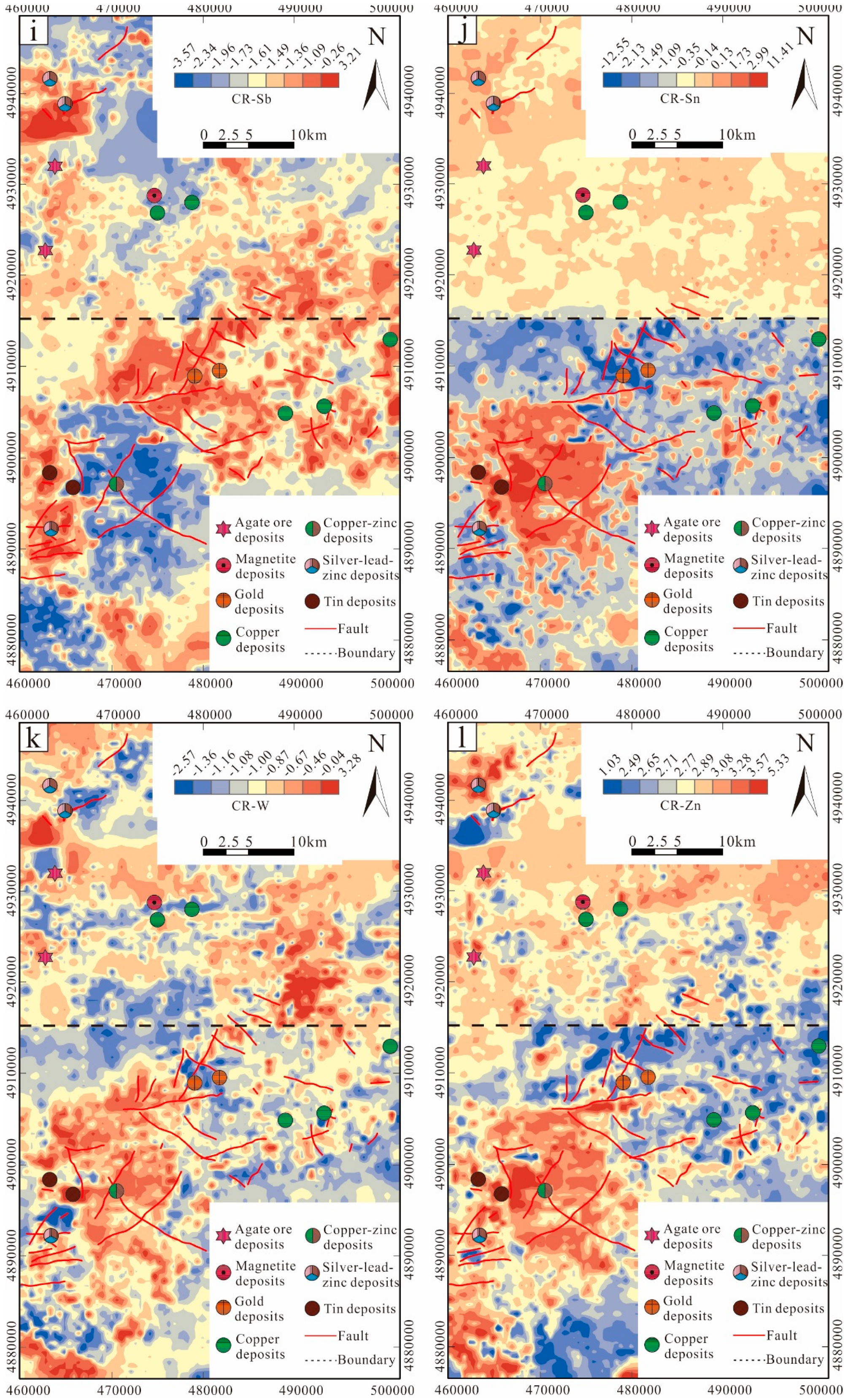
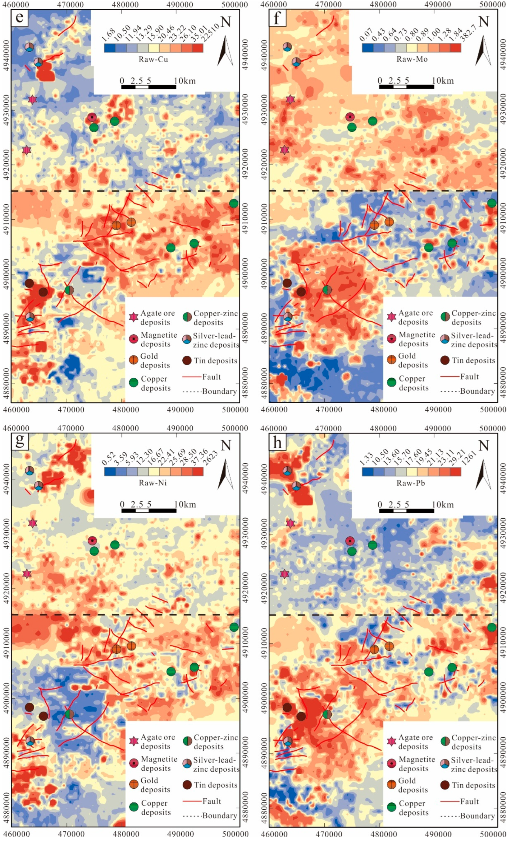
From Table 6, it can be observed that after the CR method transformation using the median, the percentiles of each element are now much closer, and the kurtosis and skewness of all elements have not changed. When considering the corresponding geochemical maps (Figure 10), the results show some improvement compared to the raw data (Figure 7). The shift effect that was present in the raw data for Ag, Mo, and Sb elements has mostly been improved. Among them, Ag and Sb elements show the best results, with almost no shift between map sheets, and the distribution of geochemical anomalies is highly consistent with the distribution of faults, reflecting the fact that faults serve as migration channels for hydrothermal fluids.

Furthermore, although Mo elements have improved to some extent, there is still a noticeable shift at the boundaries. This may be due to the fact that the CR method levels the data as a whole for each map sheet, without considering the different geochemical backgrounds caused by the large area of the study region.

Additionally, a new issue emerged after applying the CR method: data that did not originally exhibit a shift now show one. This is most notable for Sn and Bi elements, followed by Co and Ni elements, which also exhibit a shift problem. Since Bi and Sn elements are mainly related to hydrothermal activity in the study area, and the southern region has a large number of faults, which are suitable migration channels for hydrothermal fluids, the anomalous distribution in the southern region should be more prominent than in the northern region, with a higher lower limit for the geochemical background. However, the CR method directly assumes that the northern and southern regions have the same background value, leading to data errors. For Co and Ni elements, which are related to basic rocks, and given that the upwelling of basic magma provides a heat source, similar to Sn and Bi elements, there are certain background value differences between the northern and southern regions.

5.3.2. Results of the BL Method

Theoretically, data that are closer to the boundary line should be more similar (since the data comes from the same geological unit). Therefore, data close to the boundary line should be selected as much as possible. However, it is also important to consider the statistical validity of the data. Too few data points may not adequately represent the true distribution characteristics, while too many data points may deviate from the similar background.

To address this, the southern and northern boundary lines were selected with distances ranging from 500 to 5000 meters, incrementing by 500 meters. The percentiles for different boundary ranges in the northern and southern regions were calculated, and the differences in percentiles were measured using a difference metric (D-value) and displayed in a line chart to assess the degree of difference in percentiles for different boundary ranges (Figure 11).

From Figure 11, it can be seen that at a 1000 m distance, the data difference between the northern and southern regions is the smallest, meaning the similarity is highest. Therefore, the data within this range is selected as the parameter for BL.

In the boundary-based leveling process, a certain area needs to be designated as the “standard area”, and the data from other areas are then leveled based on this “standard area” using the fitting function determined by the percentiles. Since the data for each map sheet follow sampling specifications, any area can be randomly selected as the “standard area”. In this study, the southern region was chosen as the standard area because its larger sample size helps effectively reduce errors caused by insufficient samples or data fluctuations, thus improving the reliability of the leveling results. Therefore, the southern region’s data is used to adjust the northern region’s data.

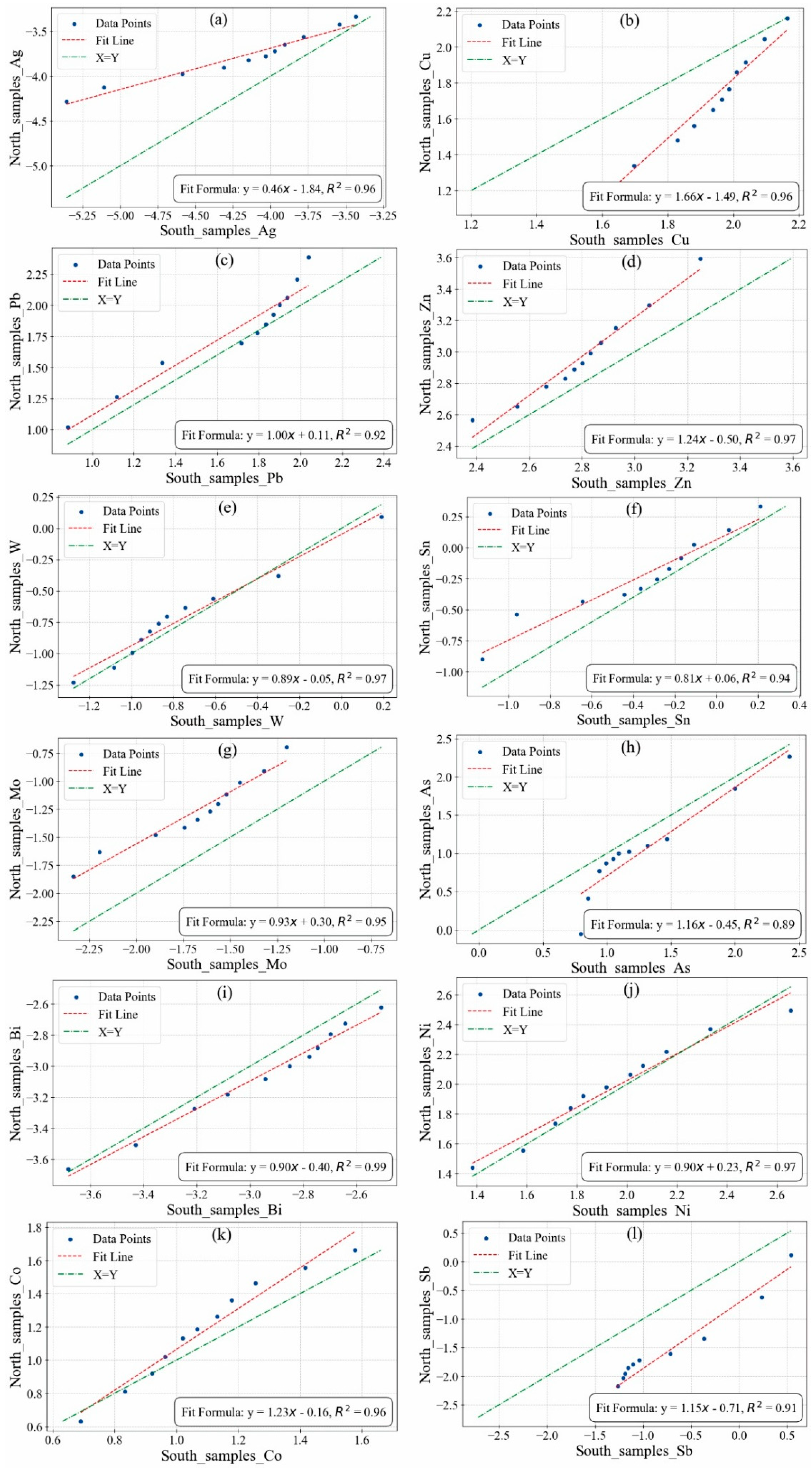
The leveling parameters are derived from the percentiles of the data within the 1000 m boundary range, and the fitting information can be seen in

Table 7. Fitted curve parameters for each element within the 1000 m north–south range for BL.

Elements	Formula	R2
Ag	y = 0.43x − 2.06	0.93
Cu	y = 1.49x − 1.14	0.96
Pb	y = 0.95x − 0.17	0.90
Zn	y = 1.19x − 0.37	0.95
W	y = 0.99x + 0.00	0.98
Sn	y = 0.72x − 0.04	0.95
Mo	y = 0.85x + 0.11	0.94
As	y = 1.25x − 0.57	0.90
Bi	y = 0.88x − 0.49	0.98
Ni	y = 0.94x + 0.10	0.98
Co	y = 1.16x − 0.11	0.96
Sb	y = 1.19x − 0.69	0.93

and Figure 12. It is clearly evident that the element Ag requires the most leveling; theoretically, the distribution curve near the boundary line should be close to X = Y, but it deviates significantly, which is worth noting. Additionally, the R² values for the elements indicate that the fitting in both the northern and southern regions is quite good (all above 0.9), showing that the data for each element in both regions exhibit linear correlation, making boundary-based leveling a viable approach.

The leveling parameters determined through the boundary were extended to the entire region, with the data from the southern region used as the baseline to level the data from the northern region. The statistics of the leveled data parameters for each region are shown in

Table 8. Statistical characteristics of the data after BL.

Element	Region	Min	25%	50%	75%	Max	StdDev	Mean	Kurt	Skew
Ag	North	−5.21	−4.01	−3.86	−3.68	−0.24	0.35	−3.83	12.86	1.79
	South	−6.28	−4.07	−3.86	−3.65	0.27	0.49	−3.86	6.36	0.54
Cu	North	−0.06	1.71	1.87	2.07	4.68	0.42	1.90	4.50	0.65
	South	−0.03	1.76	1.87	1.96	5.72	0.28	1.86	17.11	1.34
Pb	North	0.21	1.62	1.83	2.01	3.80	0.34	1.81	2.12	−0.07
	South	−1.43	1.71	1.83	2.11	4.49	0.47	1.87	4.35	−0.46
Zn	North	1.01	2.81	2.94	3.09	5.21	0.31	2.97	5.77	1.18
	South	0.91	2.84	2.94	3.22	5.31	0.36	3.03	4.37	0.78
W	North	−2.28	−1.11	−0.86	−0.60	2.84	0.51	−0.80	9.15	2.13
	South	−2.56	−0.95	−0.86	−0.66	3.05	0.38	−0.77	6.21	1.44
Sn	North	−1.60	−0.34	−0.19	0.01	2.56	0.43	−0.10	6.66	2.01
	South	−4.12	−0.40	−0.19	0.49	3.81	0.64	0.01	2.02	0.71
Mo	North	−5.25	−1.60	−1.41	−1.22	0.95	0.39	−1.41	8.84	−0.40
	South	−3.79	−1.52	−1.41	−1.11	3.08	0.51	−1.29	1.36	0.55
As	North	−1.54	0.72	0.98	1.20	5.37	0.58	0.99	5.52	0.96
	South	−2.39	0.80	0.98	1.14	5.06	0.51	1.01	5.85	1.30
Bi	North	−4.90	−3.03	−2.85	−2.64	−0.35	0.37	−2.82	5.59	1.08
	South	−5.27	−3.04	−2.85	−2.72	3.24	0.59	−2.86	12.76	1.71
Ni	North	−1.06	1.68	1.90	2.10	4.72	0.40	1.88	4.53	−0.03
	South	−1.91	0.96	1.90	2.09	5.98	0.76	1.61	0.95	−0.57
Co	North	−2.23	0.88	1.07	1.26	2.84	0.36	1.06	6.78	−0.83
	South	−3.49	0.30	1.07	1.22	3.84	0.72	0.79	1.28	−0.73
Sb	North	−2.53	−1.50	−1.35	−1.18	2.80	0.46	−1.29	12.20	2.52
	South	−3.31	−1.53	−1.35	−1.19	2.92	0.66	−1.30	4.48	1.39

.

Similarly, the data leveled using the BL method was subjected to IDW interpolation, and the results are shown in Figure 13.

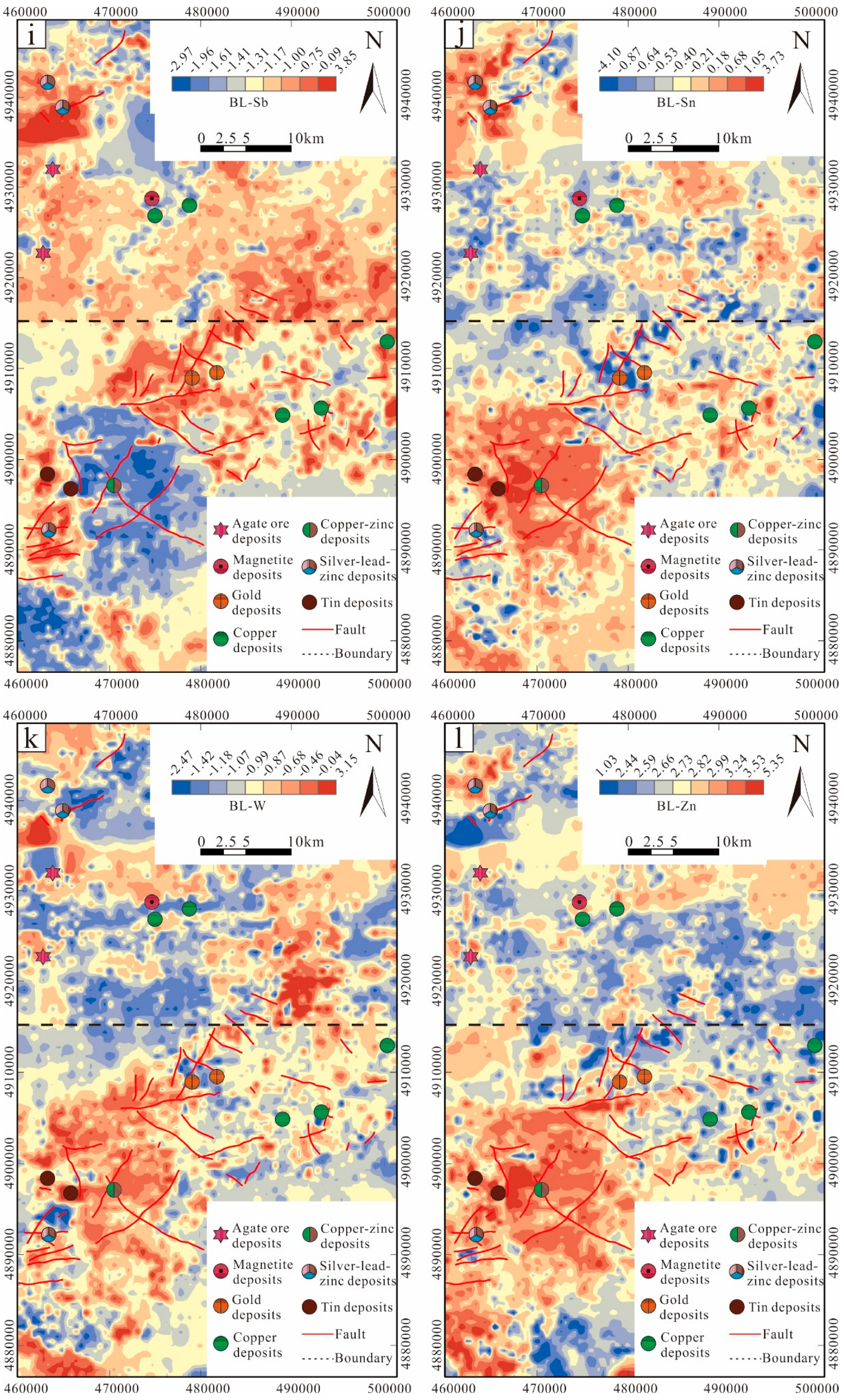
From Figure 13, it can be seen that none of the element anomaly maps exhibit a shift effect. Taking the Sb element as an example, its geochemical distribution pattern is very similar to that of As, which is also a low-temperature element. Both exhibit a significant large-scale anomaly in the northern region, with relatively fewer anomalies in the southern region. On the other hand, elements such as W, Sn, Mo, and Bi, which are associated with high-temperature hydrothermal fluids, are mainly concentrated in the southern part of the study area, closely related to the positions of intrusive or extrusive rocks. Moreover, almost all the elements’ extension orientations are close to NE, consistent with the main fault orientations in the study area.

From the distribution of mineral points, the high-concentration anomalies of Cu in the geochemical map, after being leveled by the BL method, align well with the known mineral points. Compared to the CR method, there is almost no shift, indicating that the data leveling effect is good. For Sn, the improvement is most noticeable; in the raw data, no shift was observed for Sn, but after applying the CR method, a clear boundary appeared between the northern and southern regions. Clearly, this method is not suitable for this type of data. After processing with the BL method, the Sn element geochemical anomaly map performs well, with no shift and a large-scale anomaly in the southern region. This aligns with the geological background of widespread extrusive rocks in the southern region of the study area, confirming the good leveling effect of the BL method.

5.3.3. Results of MSC Method

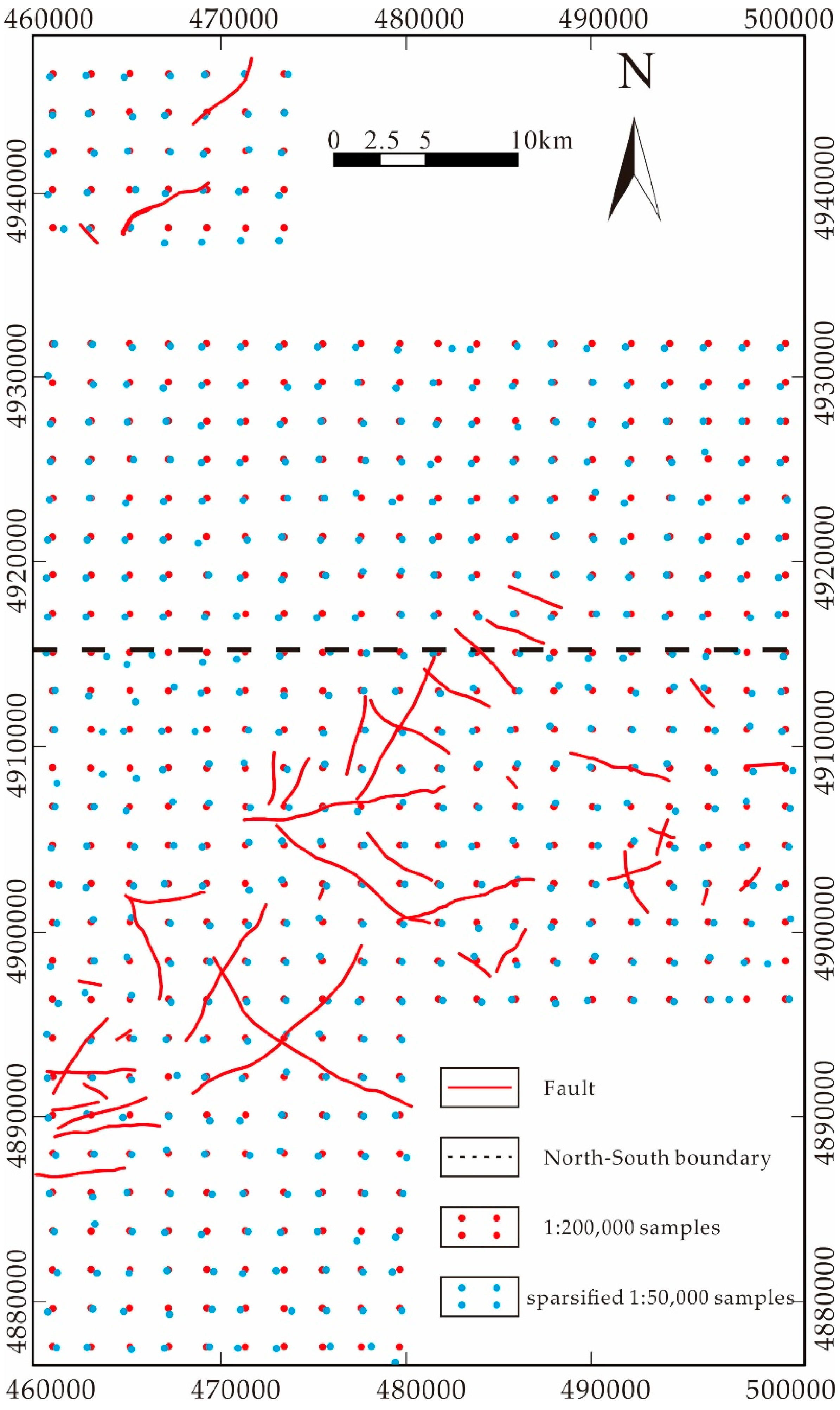
Using the 1:200,000 geochemical data as the calibration medium, the sparsified 1:50,000 data for both the northern and southern regions were leveled to their corresponding levels. Then, the corrected relationships obtained from the sparsified data were applied to all the data, offering another approach to processing. Essentially, this method assumes that the 1:200,000 data serves as the baseline at the same or nearby sampling locations, and thus, the 1:50,000 data (including both the northern and southern regions) is leveled accordingly.

By calculating the Euclidean distance, the closest 1:50,000 sampling point to each 1:200,000 sampling point was selected. As shown in Figure 14, the distributions of the sparsified 1:50,000 sampling points and 1:200,000 sampling points are nearly identical. Comparing the distribution of the sparsified samples, it can be concluded that the sampling locations are essentially the same. This means that for single elements, such as the Ag element in the northern region, the data from 1:200,000 should closely align with the data from 1:50,000, and the fitting curve of the percentiles should show a slope of 1, corresponding to the X = Y distribution.

However, in practice, there is still some systematic error. Therefore, we can correct this systematic error using the slope and intercept. Furthermore, the parameters for the slope and intercept apply to the entire northern 1:50,000 data set, and not just the sparsified data.

First, the fitting parameters between the sparsified 1:50,000 data and the 1:200,000 data were calculated. The fitting results are shown in the

Table 9. Fitted curve parameters for each element within the 1000 m north–south range.

	Elements	Formula	R2
north	Ag	y = 2.08x + 4.12	0.98
	Cu	y = 2.53x − 2.81	0.85
	Pb	y = 1.59x − 1.11	0.98
	Zn	y = 1.73x − 2.31	0.98
	W	y = 1.38x + 0.46	0.98
	Sn	y = 2.28x + 0.57	0.98
	Mo	y = 2.16x + 1.51	0.99
	As	y = 1.42x − 0.13	0.98
	Bi	y = 2.34x + 4.30	1.00
	Ni	y = 1.90x − 2.36	0.99
	Co	y = 2.09x − 1.96	1.00
	Sb	y = 1.96x + 2.14	0.95
south	Ag	y = 1.08x + 1.10	0.92
	Cu	y = 1.81x − 1.84	0.93
	Pb	y = 1.44x − 0.81	0.91
	Zn	y = 1.21x − 0.55	0.87
	W	y = 1.65x + 0.70	0.97
	Sn	y = 0.97x + 0.50	0.91
	Mo	y = 1.26x + 0.65	0.85
	As	y = 1.72x − 0.95	0.94
	Bi	y = 1.40x + 1.29	0.86
	Ni	y = 1.14x − 0.93	0.87
	Co	y = 0.95x − 0.26	0.84
	Sb	y = 1.73x + 0.33	0.89

(since the table and figure provide the same information, they are not displayed here). From the R² values, which are consistently above 0.85, it is evident that the linear relationship is strong, and leveling based on the 1:200,000 data is valid.

Similar to the data after BL, the percentiles of all elements are also very close after the MSC method. The specific parameters are shown in

Table 10. Statistical characteristics of the data after MSC.

Element	Region	Min	25%	50%	75%	Max	StdDev	Mean	Kurt	Skew
Ag	North	−6.17	−3.81	−3.51	−3.16	3.64	0.68	−3.45	12.86	1.79
	South	−5.93	−3.46	−3.22	−2.98	1.40	0.55	−3.21	6.36	0.54
Cu	North	−2.94	1.09	1.45	1.90	7.88	0.97	1.53	4.50	0.65
	South	−1.90	1.44	1.63	1.81	8.80	0.53	1.63	17.11	1.34
Pb	North	−0.78	1.44	1.78	2.06	4.89	0.54	1.74	2.12	−0.07
	South	−2.88	1.66	1.83	2.23	5.68	0.68	1.89	4.35	−0.46
Zn	North	−0.52	2.66	2.89	3.15	6.91	0.55	2.95	5.77	1.18
	South	0.54	2.85	2.96	3.30	5.79	0.43	3.07	4.37	0.78
W	North	−2.55	−1.01	−0.68	−0.34	4.22	0.67	−0.60	9.15	2.13
	South	−3.57	−0.88	−0.73	−0.39	5.78	0.63	−0.57	6.21	1.44
Sn	North	−3.20	−0.23	0.12	0.60	6.59	1.02	0.34	6.66	2.01
	South	−3.37	0.13	0.32	0.96	4.08	0.60	0.50	2.02	0.71
Mo	North	−7.99	−1.38	−1.04	−0.70	3.24	0.71	−1.04	8.84	−0.40
	South	−4.60	−1.46	−1.30	−0.89	4.91	0.70	−1.13	1.36	0.55
As	North	−2.20	0.85	1.20	1.50	7.12	0.78	1.20	5.52	0.96
	South	−5.14	0.44	0.77	1.04	7.92	0.89	0.81	5.85	1.30
Bi	North	−8.52	−3.62	−3.14	−2.59	3.39	0.98	−3.07	5.59	1.08
	South	−5.80	−2.80	−2.54	−2.37	5.65	0.80	−2.56	12.76	1.71
Ni	North	−4.46	0.98	1.42	1.82	7.02	0.80	1.38	4.53	−0.03
	South	−3.05	0.14	1.19	1.40	5.71	0.84	0.86	0.95	−0.57
Co	North	−7.14	0.08	0.52	0.97	4.65	0.84	0.50	6.78	−0.83
	South	−3.38	0.01	0.69	0.83	3.17	0.64	0.45	1.28	−0.73
Sb	North	−4.73	−1.93	−1.51	−1.06	9.73	1.24	−1.37	12.20	2.52
	South	−4.93	−2.10	−1.81	−1.56	4.97	1.05	−1.74	4.48	1.39

.

It should be emphasized that even though the 1:50,000 and 1:200,000 data were analyzed using different detection methods, it does not affect the leveling process. This is because, through linear regression, we focus on the trends or ratios between the data. As long as the data does not contain non-systematic errors, there will always be a clear linear relationship between the measurement values, and therefore, leveling can be performed using linear regression.

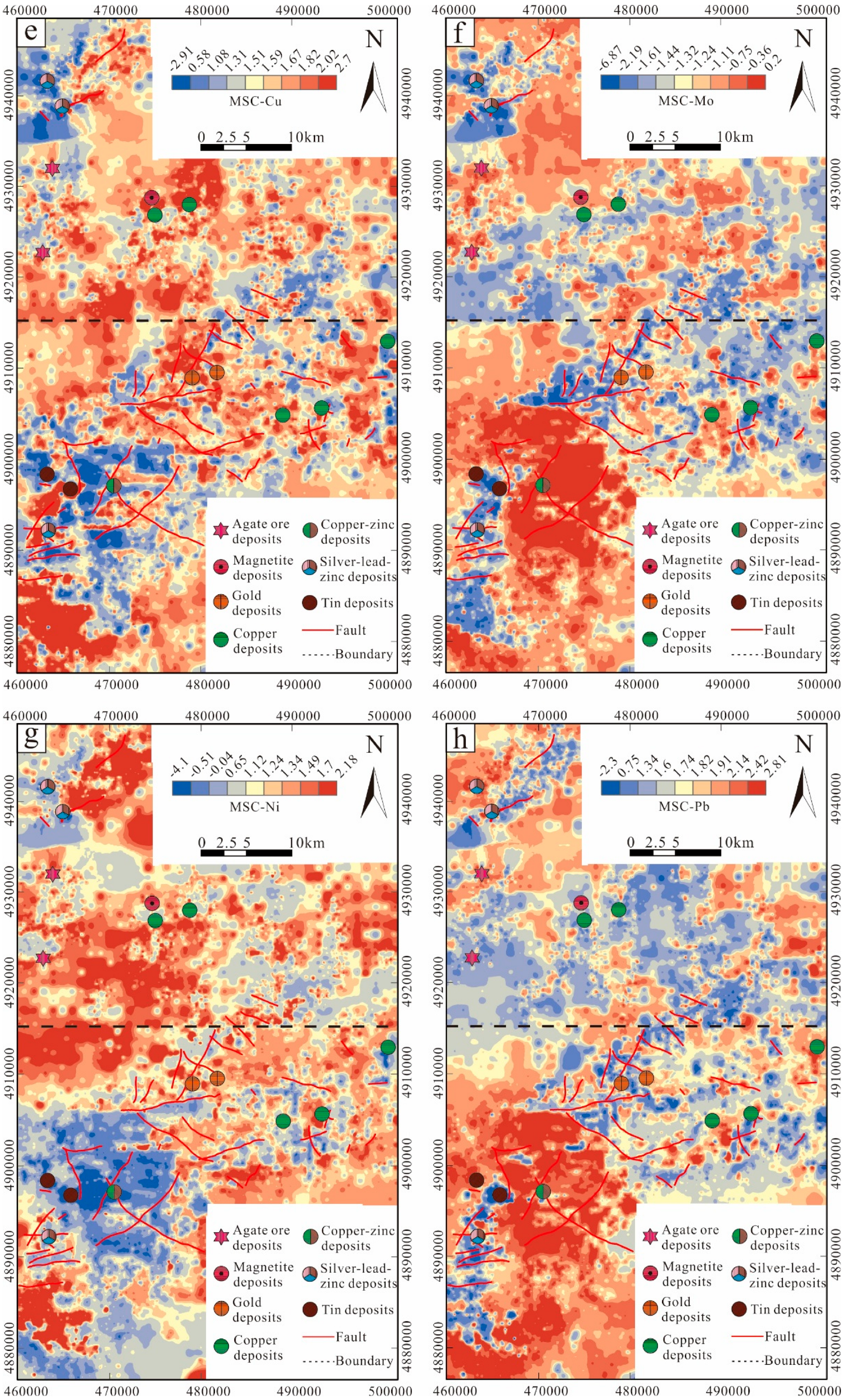
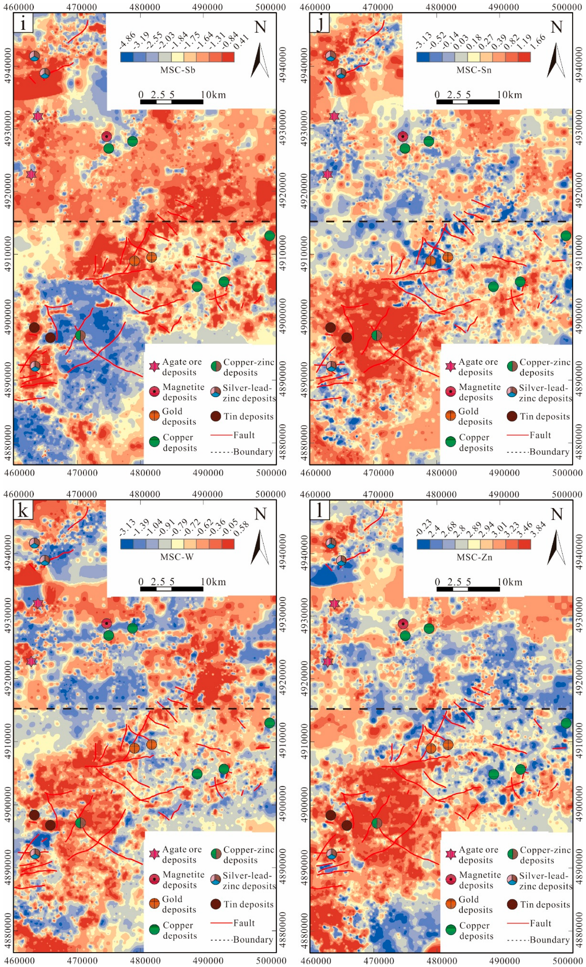
The results of the MSC method, as shown in Figure 15, are essentially consistent with the BL method. Most of the elements are improved to some extent, and no issues similar to those in the CR method were observed. Since the geochemical map distribution is essentially consistent with that of the BL method, no further explanation is provided here.

5.4. Comparison Results and Discussion of Various Methods

5.4.1. Necessity and Practicality of Data Leveling

Geochemical data leveling is especially important in mineral exploration because it directly affects the accuracy and efficiency of mineral resource assessment. During the exploration process, data typically come from vast geographical areas and different time periods, with multiple teams using various methods and instruments for sampling and analysis. Due to these differences, unleveled data can mislead interpretation, leading to overestimation or underestimation of resource potential.

Necessity: In mineral exploration, data leveling is necessary because it directly impacts the consistency and reliability of the data. Since exploration data often come from different time periods, different technical teams, and various instruments, unadjusted data may have significant systematic biases, such as differences in detection limits and measurement errors. These uncorrected biases can lead to misinterpretations of geochemical signals, especially when comparing the concentrations of ore-forming elements, potentially overlooking actual geological anomalies or mistakenly identifying normal backgrounds as anomalies. Data leveling eliminates these differences, ensuring that all data are evaluated and interpreted on the same baseline, improving the comparability of data across regions, thus providing accurate scientific evidence for mineral exploration.

Practicality: From a practical perspective, data leveling enhances the application value of geochemical data in the exploration process. Leveled data are more suitable for generating geochemical anomaly maps and conducting multi-element correlation analysis, which are key tools for identifying potential mineralized areas. For instance, adjusted data can more accurately depict the surface distribution patterns of metallic elements, helping geologists pinpoint hotspot areas of mineralization, thereby guiding field exploration and drilling activities. Moreover, leveled data are crucial for establishing and applying geochemical exploration models, which can effectively predict and assess future mineral potential, thus providing quantitative support for exploration decisions. The enhanced accuracy and reliability of leveled data significantly improve resource utilization efficiency, reduce exploration risks, and provide a solid scientific foundation for mineral development.

5.4.2. Selection Among Various Methods

During the preliminary research, we found that geologists have proposed multiple leveling methods, each suitable for different data characteristics. Among these, the most widely used method is the CR method, which is applicable to most data leveling tasks. However, it still has limitations. For instance, in small-scale map sheets, the large area covered by the map sheet often spans different geological units or even geochemical landscapes. As a result, if one map sheet is treated as a whole for leveling, errors may arise.

The BL method is based on the assumption that the element distribution pattern within the same geological unit should be similar. The difficulty lies in selecting the appropriate boundary range, and its applicability is also limited—requiring the geological units at the boundary to be continuous. Despite these limitations, findings indicate that this method can be applied to both large-scale and small-scale maps, suggesting its reliability may be higher than that of the CR method.

The MSC method yields results similar to those of the BL method. However, it does not require considering differences between boundary geological units, making it less restricted and more widely applicable. However, it does require the availability of geochemical data at multiple scales.

6. Conclusions

In this study, the leveling of geochemical data was performed using the CR method, BL method, and MSC method after compositional data transformation. The following conclusions were drawn:

• Between multiple map sheets, inherent differences due to factors such as different units, different time periods, and different instruments may cause a shift effect in geochemical data. Therefore, data leveling is necessary to improve the data’s usability and accuracy.
• The CR method is not suitable for leveling in areas with small scales or significant geological background differences.
• The BL method works well in eliminating the shift for all elements and is applicable for leveling between different scales. However, its limitation is that the geological conditions at the boundaries need to be consistent.
• The MSC method yields results similar to the BL method but does not require consistent boundary conditions, making it less restricted. However, it requires geochemical data at multiple scales.

In summary, this paper used the uneven distribution of geochemical anomalies between multiple map sheets in the Baiyinchagan–Maodeng area as a starting point, thoroughly analyzing various methods for handling the “shift” in geochemical data. When confronted with such data exhibiting “shift”, it is crucial to first perform compositional data transformation to eliminate the closure effect inherent in the data. Subsequently, the optimal data leveling methods should be explored, prioritizing the use of similarities between geological boundaries and potentially incorporating data at different scales to achieve effective data leveling. This exploration aims to provide a valuable reference for future explorers need to address similar issues.