A Novel Method for Traffic Parameter Extraction and Analysis Based on Vehicle Trajectory Data for Signal Control Optimization

Abstract

As urban traffic systems become increasingly complex, traditional traffic data collection methods based on fixed detectors face challenges such as poor data quality and acquisition difficulties. Traditional methods also lack the ability to capture complete vehicle path information essential for signal optimization. While vehicle trajectory data can provide rich spatiotemporal information, its sampling characteristics present new technical challenges for traffic parameter extraction. This study addresses the key issue of extracting traffic parameters suitable for signal timing optimization from sampled trajectory data by proposing a comprehensive method for traffic parameter extraction and analysis based on vehicle trajectory data. The method comprises five modules: data preprocessing, basic feature processing, exploratory data analysis, key feature extraction, and data visualization. An innovative algorithm is proposed to identify which intersections vehicles pass through, effectively solving the challenge of mapping GPS points to road network nodes. A dual calculation method based on instantaneous speed and time difference is adopted, improving parameter estimation accuracy through multi-source data fusion. A highly automated processing toolchain based on Python and MATLAB is developed. The method advances the state of the art through a novel polygon-based trajectory mapping algorithm and a systematic multi-source parameter extraction framework specifically designed for signal control optimization. Validation using actual trajectory data containing 2.48 million records successfully eliminated 30.80% redundant data and accurately identified complete paths for 7252 vehicles. The extracted multi-dimensional parameters, including link flow, average speed, travel time, and OD matrices, accurately reflect network operational status, identifying congestion hotspots, tidal traffic characteristics, and unstable road segments. The research outcomes provide a feasible technical solution for areas lacking traditional detection equipment. The extracted parameters can directly support signal optimization applications such as traffic signal coordination, timing optimization, and congestion management, providing crucial support for implementing data-driven intelligent traffic control. This research presents a theoretical framework validated with real-world data, providing a foundation for future implementation in operational signal control systems.

1. Introduction

1.1. Research Background

With the continuous acceleration of urbanization, urban traffic systems face unprecedented pressure and challenges. The high concentration of urban population, frequent economic activities, and accelerated personnel mobility have brought rapid economic and social development while also causing severe traffic congestion problems. Traffic congestion not only leads to reduced vehicle speeds in urban areas and increased travel time with greater uncertainty, but also results in increased fuel consumption, higher pollutant and greenhouse gas emissions, and increased road accident rates, among other serious socioeconomic impacts.

Since the world’s first traffic signal was installed in the Westminster area of London, England, in 1868, urban traffic control has developed over more than 150 years. As the primary means for cities to alleviate road congestion and rationally allocate road network resources, the importance of traffic signal control has become increasingly prominent. Fixed-time signal control adopts pre-determined periodic control schemes designed for specific scenarios and optimized offline. However, traditional signal control optimization heavily relies on accurate traffic flow data input, and obtaining such data faces numerous challenges.

Traditional traffic data collection mainly relies on fixed detectors, including inductive loop detectors, radar detectors, and video detectors. Although these detection devices are technologically mature, they have numerous limitations. First, the installation and maintenance costs of the equipment are high, requiring regular inspection and replacement. Second, fixed detectors have limited spatial coverage and can only obtain cross-sectional data, making it difficult to reflect complete vehicle trajectories. Third, data quality is susceptible to environmental factors such as weather conditions and equipment aging. Fourth, these devices have difficulty obtaining complete vehicle path information and cannot provide fine-grained traffic flow characteristics.

1.2. Research Significance

With the rapid development of traffic data collection technology, traffic data collection methods have become increasingly diversified, and both the types and volume of traffic data have been greatly enriched. Supported by abundant traffic data, the entire traffic control field has evolved from the data-sparse era to the data-rich era. Control methods are gradually transitioning from statistical data-based modeling approaches to data-driven directions. Model-free intelligent control methods have naturally become a hot topic in the field. Therefore, more and more scholars are beginning to abandon traditional thinking and address a series of traffic control problems within unified intelligent control algorithm frameworks, bringing unprecedented possibilities to traffic control.

Vehicle trajectory data, represented by GPS-equipped taxis, ride-hailing vehicles, connected and automated vehicles, and digital map navigation vehicles, serves as an emerging traffic data source with incomparable advantages over traditional detector data. The complete physical trajectory of vehicles during travel not only reflects the vehicle’s path on the road network but also reveals the spatiotemporal variation characteristics of vehicle speed. It represents the most comprehensive and complete expression of traffic flow operational status, containing extremely rich traffic flow information such as travel time and speed, queue length, delay, and multiple stops. This information holds significant value for understanding both microscopic and macroscopic traffic flow characteristics and optimizing signal control strategies.

However, trajectory data is essentially sampled data, characterized by limited penetration rates, varying data quality, and uneven spatiotemporal coverage. How to accurately extract traffic parameters from limited trajectory samples and effectively apply these parameters to signal control optimization is a technical problem with significant theoretical and practical value. Particularly in the context where traditional traffic detection equipment yields poor data quality at high costs, traffic parameter extraction methods based on trajectory data provide a new technical pathway for traffic signal control optimization.

1.3. Literature Review

Accurately and timely obtaining microscopic and macroscopic traffic flow characteristic parameters and evolution trends forms the foundation for traffic control strategy optimization, evaluation, and feedback. While this study focuses primarily on vehicle trajectory data for signal control optimization, it is important to acknowledge the broader multi-modal transportation context. Urban traffic systems encompass various transportation modes, including pedestrians, cyclists, public transit, and emerging mobility services. Pedestrian and cyclist movements at signalized intersections significantly influence signal timing requirements, particularly for crossing phases and all-red clearance intervals. However, the current research scope is specifically designed for vehicle-based signal control optimization, as vehicle trajectories provide the most direct input for traditional traffic signal timing parameters such as flows, speeds, and coordination offsets. Future extensions of this methodology could incorporate pedestrian detection data and bicycle trajectory information to support comprehensive multi-modal signal control strategies.

Currently, research on traffic parameter extraction based on vehicle trajectory data mainly focuses on the following aspects:

Regarding link speed estimation, researchers have proposed various speed estimation methods based on trajectory data. Ni and Wang developed a trajectory reconstruction model using smoothing schemes to construct speed surfaces, achieving 6.3% mean absolute percentage error compared to ground truth [1]. Cao et al. proposed real-time vehicle trajectory prediction using deep neural networks for traffic conflict detection at unsignalized intersections [2]. Shang et al. demonstrated that multisource data-based dynamic methods significantly outperformed static approaches in freeway traffic state estimation [3]. Lai et al. achieved 95.72% accuracy in vehicle speed forecasting using cellular floating vehicle data combined with neural network algorithms [4]. Early methods primarily involved simple average speed calculations, later evolving to include estimation methods considering spatiotemporal correlations and machine learning-based prediction models. Li et al. developed post-earthquake traffic travel time distribution estimation methods based on floating car data with reliability analysis [5]. These methods have achieved remarkable results in single-indicator speed and travel time estimation, providing a solid technical foundation for further construction of network-wide state assessment systems.

In travel mode identification, research mainly focuses on identifying different transportation modes from trajectory data (such as walking, cycling, driving, and public transit) and trip purposes (such as commuting, shopping, and leisure). Zheng et al. pioneered supervised learning approaches for transportation mode learning from raw GPS data using change point-based segmentation [6]. Li et al. enhanced transportation mode identification to 91.1% accuracy by incorporating GIS information with GPS trajectory data [7]. Sadeghian et al. provided a comprehensive review and evaluation of GPS-based transport mode detection methods [8]. Zeng et al. proposed a novel trajectory-as-a-sequence framework for travel mode identification using sequence-to-sequence models [9]. James achieved superior performance using wavelet transform and deep learning for GPS trajectory-based travel mode identification [10]. Sadeghian et al. developed deep semi-supervised machine learning algorithms, achieving 93.94% accuracy with minimal labeled data [11]. Ma et al. introduced multi-stage fusion networks with varied scale representation for transportation mode identification [12]. These studies provide important information for understanding urban traffic demand while offering rich user behavior data support for intelligent signal control systems, facilitating more precise traffic management decisions.

For OD matrix reconstruction, traditional methods mainly rely on traffic survey data, which is costly with long update cycles. Zhou and Mahmassani introduced dynamic origin–destination demand estimation using automatic vehicle identification data without requiring market-penetration rates [13]. Rao et al. developed origin–destination pattern estimation based on trajectory reconstruction using automatic license plate recognition data, achieving MAPEs lower than 19% [14]. OD matrix estimation methods based on trajectory data can provide dynamic, real-time OD information. Shi et al. enhanced travel time prediction through high-resolution origin-destination approaches with multi-dimensional features, achieving an RMSE of 202.89 s [15]. Through continuously optimized data processing algorithms and statistical modeling techniques, significant progress has been made in addressing data sparsity and bias issues, providing a more reliable data foundation for traffic planning and management.

In traffic congestion detection and prediction, researchers have utilized the spatiotemporal characteristics of trajectory data to develop various congestion identification algorithms. Sun et al. demonstrated that deep learning models significantly outperformed conventional machine learning in traffic congestion prediction based on GPS trajectory data [16]. Kong et al. proposed urban traffic congestion estimation and prediction methods using floating car trajectory data with fuzzy comprehensive evaluation [17]. Qu et al. studied catastrophe boundary extraction and the evolution of expressway traffic flow states [18]. Ranjan et al. developed a large-scale road network traffic congestion prediction based on recurrent high-resolution networks [19]. Kumar and Raubal provided a comprehensive survey of deep learning applications in congestion detection, prediction and alleviation [20]. These methods can monitor network congestion status in real time and, combined with advanced data fusion techniques and intelligent decision-making algorithms, are evolving toward complete congestion warning and control strategy generation systems, providing strong technical support for implementing proactive traffic management.

However, existing research still has deficiencies in the following aspects. First, there is a lack of systematic data preprocessing methods, resulting in inconsistent data quality. Second, the accuracy of trajectory point-to-road network matching needs improvement, affecting the accuracy of subsequent parameter extraction. Third, the consistency and accuracy issues in multi-parameter extraction have not been well resolved. Fourth, the reusability and practicality of methods need improvement, as many research outcomes are difficult to apply in practical engineering.

1.4. Contributions

Addressing the deficiencies in existing research, this study proposes a comprehensive framework for traffic parameter extraction and analysis based on vehicle trajectory data. The main contributions include:

(1)

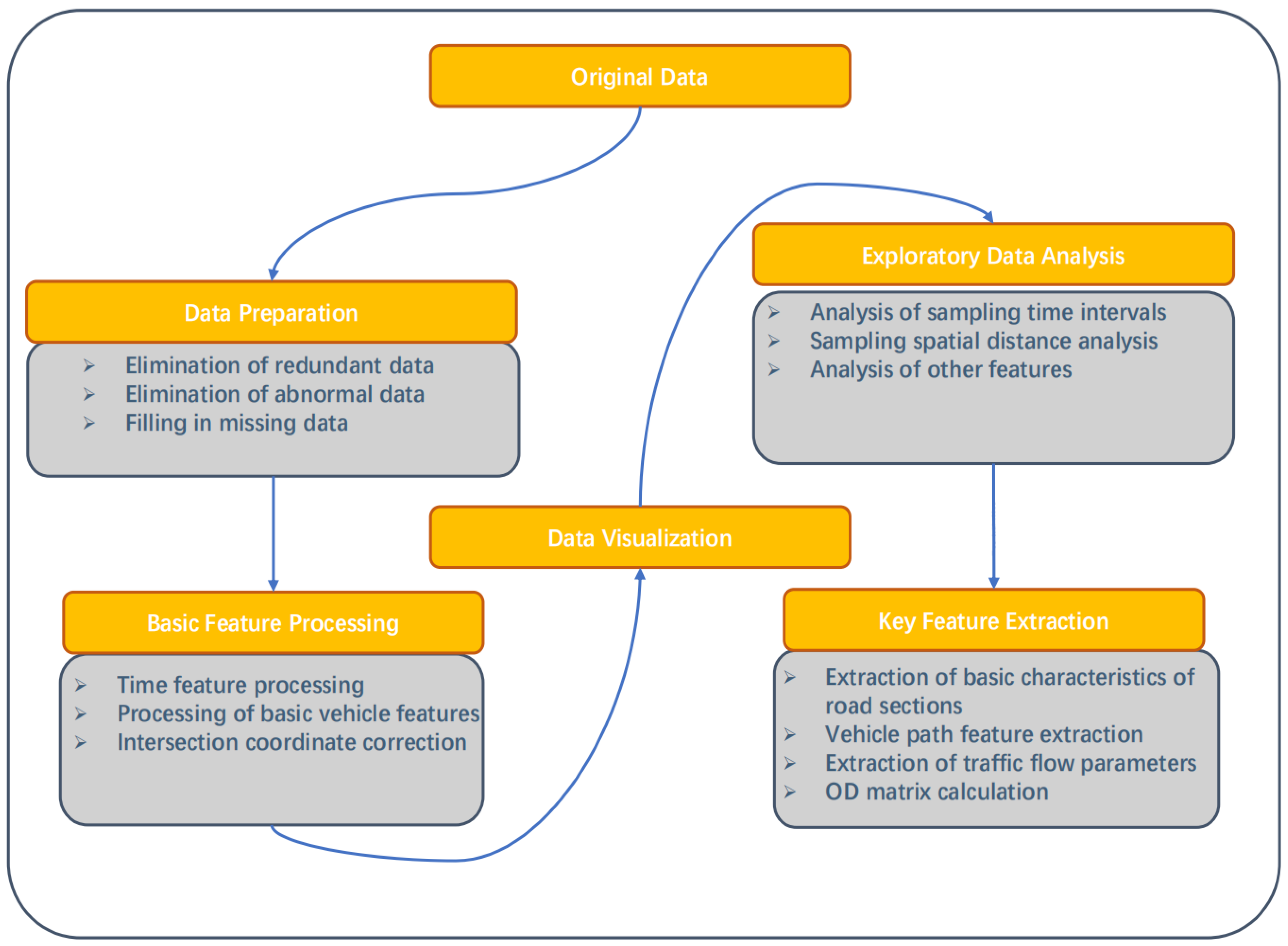
Established a systematic trajectory data processing methodology framework. This study designs a complete processing workflow including data preprocessing, basic feature processing, exploratory data analysis, key feature extraction, and data visualization. Each module has been carefully designed and optimized to ensure data processing quality and efficiency. The framework exhibits excellent modular characteristics with clear interfaces between modules, facilitating customization and extension according to specific requirements.

(2)

Proposed a trajectory point “labeling” algorithm based on regular polygon coverage. This effectively solves the technical challenge of mapping discrete trajectory points to road network nodes. By constructing regular polygon coverage areas centered on nodes and utilizing geometric determination algorithms to assign trajectory points, high-precision vehicle path identification is achieved. The algorithm demonstrates excellent stability and efficiency when processing large-scale data.

(3)

Established a multi-source data fusion method for traffic parameter calculation. Addressing the uncertainty in trajectory data, this study adopts a dual calculation method based on vehicle instantaneous speed and arrival time differences, improving parameter extraction accuracy and reliability through multi-source information fusion. This method effectively reduces errors that may arise from single data sources and enhances the robustness of parameter estimation.

(4)

Developed a highly reusable and automated data processing toolchain. Based on Python and MATLAB platforms, a series of comprehensive data processing functions and modules have been developed, including automated data cleaning, feature extraction, parameter calculation, and result visualization. These highly reusable and automated tools not only serve this research but can also provide technical support for other researchers and engineering practices.

(5)

Validated the effectiveness of the method through actual data. Using actual trajectory data containing over 2.48 million records, the performance of the proposed method was comprehensively validated. Experimental results demonstrate that the method can effectively process large-scale data, and the extracted traffic parameters accurately reflect the operational status of the road network, providing a reliable data foundation for signal control optimization.

2. Methodology

2.1. Overall Framework

The proposed methodology framework is specifically designed to address the core requirements of traffic signal control optimization, which demands accurate, reliable, and comprehensive traffic parameters, including link flows, travel times, speeds, and OD matrices. Each module serves distinct optimization objectives: data preprocessing ensures data quality essential for reliable signal timing calculations; basic feature processing provides temporal and spatial calibration necessary for coordination control; exploratory analysis identifies traffic patterns crucial for adaptive signal strategies; key feature extraction generates the specific parameters required for signal optimization algorithms; and data visualization supports decision-making in signal control design and evaluation.

The traffic parameter extraction and analysis method based on vehicle trajectory data proposed in this study adopts a modular design philosophy, constructing a hierarchically structured and functionally comprehensive processing framework. As shown in Figure 1, the entire framework comprises five main modules: data preprocessing module, basic feature processing module, exploratory data analysis module, key feature extraction module, and data visualization module. This design not only ensures the systematicity and completeness of the processing workflow but also provides excellent scalability and reusability.

The data flow between modules is clear and explicit: raw trajectory data first undergoes cleaning and preliminary organization through the data preprocessing module, removing redundant and anomalous data; it then enters the basic feature processing module for temporal feature transformation, vehicle feature encoding, and spatial coordinate calibration; the processed data is used both for exploratory data analysis to understand basic data characteristics and distribution patterns, and enters the key feature extraction module to extract core traffic parameters such as link flow, speed, travel time, and OD matrices; finally, all results are intuitively presented through the data visualization module to support decision-making analysis.

Figure 1. Workflow of fundamental data analysis.

Figure 1. Workflow of fundamental data analysis.

2.2. Data Preprocessing

Data preprocessing forms the foundation of the entire method, with its quality directly affecting the accuracy of subsequent analyses. The data preprocessing in this study includes three main steps: redundant data removal, anomalous data removal, and missing data imputation.

2.2.1. Redundant Data Removal

During trajectory data collection and transmission, equipment or network issues often generate numerous duplicate records. These redundant data not only occupy storage space but also affect the accuracy of statistical analysis. This study designs a deduplication method based on multi-dimensional features. The deduplication algorithm considers the combined uniqueness of vehicle ID (vid), timestamp (time), and coordinate position (xcoord, ycoord). The implementation utilizes Python’s pandas library, first sorting the data according to these key fields, then using the drop_duplicates() function to remove completely identical records. This method ensures both deduplication accuracy and high processing efficiency.

The original trajectory data contained 2,487,406 records. After redundant data removal, 1,721,189 records remained, with 766,217 redundant records eliminated, accounting for 30.80% of the original data volume. This proportion indicates severe redundancy issues in the original data, validating the necessity of deduplication processing.

2.2.2. Anomalous Data Removal

Identification and removal of anomalous data constitute a critical step in data quality control. This study employs anomaly detection methods based on spatial distribution and trajectory continuity, combined with visualization techniques for manual verification.

First, the road network composed of trajectory points and intersections is visualized using the plotRoadnet() function. The visualization results clearly show one severely deviated anomalous trajectory point outside the road network range, as well as multiple trajectory points that deviate somewhat from the road network. These anomalous points may result from GPS signal drift or equipment malfunction. The manual anomaly identification process focused on clearly identifiable outliers that were visually obvious (e.g., trajectory points located tens of meters away from the road network boundary). To ensure consistency, the visual inspection was conducted by two researchers independently, with a consensus reached on all identified anomalies. For borderline cases showing minor deviations, data points were retained to avoid over-filtering. In Figure 2, the numbered labels (1–22) represent intersection identifiers, while the blue dots indicate vehicle trajectory points collected from GPS data. This visualization convention is consistently applied throughout Figure 2, Figure 3, Figure 4 and Figure 5 to maintain clarity in road network representation.

Second, the removeOutlier() function is designed to implement automated anomaly detection. This function not only identifies trajectory points with abnormal spatial positions but also detects vehicle records containing only a single trajectory point. Such vehicles lack trajectory information for effective path analysis and thus need to be removed.

While statistical outlier detection techniques such as z-score analysis or DBSCAN clustering could provide more systematic approaches, the manual visual inspection method was selected for this study due to the clear spatial nature of the anomalies and the need for domain-specific judgment in trajectory data quality assessment. Future implementations could benefit from integrating automated statistical methods for enhanced scalability and objectivity. The results after removal are shown in Figure 3, where intersections numbered 4, 5, 6, 7, 13, and 14 are not physical intersections but rather signalized pedestrian crossings.

The anomalous data processing results show that among 7317 initial vehicles, 65 vehicles had only one trajectory point. These vehicle records were completely removed, ultimately retaining 7252 valid vehicles. This processing ensures data quality for subsequent analyses.

Figure 3. Optimized road network visualization results.

Figure 3. Optimized road network visualization results.

2.2.3. Missing Data Imputation

Data completeness is an important prerequisite for ensuring analytical accuracy. This study conducted comprehensive missing value checks on the processed trajectory data. Fortunately, no missing values were found in the data after the first two processing steps, possibly due to the well-designed data collection system. Therefore, this study did not perform missing data imputation operations, but retained this module in the methodological framework to address potential missing value issues in other datasets.

2.3. Basic Feature Processing

The basic feature processing module is responsible for converting raw data into formats suitable for analysis, including three components: temporal feature processing, vehicle basic feature processing, and intersection coordinate calibration.

2.3.1. Temporal Feature Processing

Temporal information is one of the core dimensions of trajectory data. Time in the raw data is stored as Unix timestamps, which need to be converted to a human-readable format and have time period features extracted.

Through the timeSegment() function, it was detected that the data contains 10 time periods, each spanning 2 h, all during weekday morning peak hours (7:00 a.m. to 9:00 a.m.). This finding has significant implications for subsequent traffic pattern analysis, as morning peak hours represent the most congested period in urban traffic and are a key focus for signal control optimization.

2.3.2. Vehicle Basic Feature Processing

Vehicles are the fundamental units of traffic flow, and accurate identification and encoding of each vehicle’s characteristics are crucial for trajectory analysis. This study constructs a complete vehicle basic feature data table (vinfo) through the vinfoAdd() function, containing the following key information: unique vehicle identifier (vid)—a unique number assigned to each vehicle; time period assignment (timeseg)—the time period in which the vehicle appears; trajectory start and end row numbers (s_idx, e_idx)—position indices of the vehicle trajectory within the overall data.

This structured vehicle feature table not only facilitates rapid location of each vehicle’s trajectory data but also supports various complex queries and statistical operations. The recording of start and end row numbers, in particular, greatly improves the efficiency of subsequent batch processing.

2.3.3. Intersection Coordinate Calibration

The accuracy of intersection coordinates directly affects the precision of vehicle path identification. In practical application, it was found that the original intersection coordinate data deviated from the actual convergence centers of trajectory points. Without calibration, it would be impossible to correctly identify the sequence of intersections passed by vehicles. The data shows that multiple intersections exhibit varying degrees of coordinate deviation, with intersection 8 deviating by tens of meters, and other intersections showing deviations ranging from several meters to tens of meters. Such deviations may result from inconsistent coordinate systems or data entry errors.

Intersection coordinate calibration employs a semi-automated method based on trajectory data: first, road network visualization is performed using MATLAB’s plotRoad() function to intuitively display deviations between intersection positions and trajectory convergence points; then, based on trajectory density distribution, intersection coordinates are manually adjusted to trajectory convergence centers; finally, the calibration effect is verified through re-visualization. Figure 4 shows the post-calibration results, demonstrating that all intersections are accurately positioned at trajectory convergence centers, providing a foundation for subsequent path identification. In Figure 4, the asterisk (*) symbols indicate the calibrated intersection center positions after coordinate adjustment.

Figure 4. Illustration of calibrated intersection coordinate positions (no deviation occurred).

Figure 4. Illustration of calibrated intersection coordinate positions (no deviation occurred).

2.4. Vehicle Path Feature Extraction

Vehicle path feature extraction represents the core technical innovation of this study, aiming to identify the sequence of nodes (intersections and OD points) traversed by vehicles from discrete trajectory point sequences, and subsequently calculate various traffic parameters. The vehicle path feature extraction process follows a systematic four-stage workflow: Stage 1 involves OD point addition, where virtual origin–destination points are strategically placed at network boundaries to capture vehicle entry and exit behaviors; Stage 2 implements regular polygon generation, creating coverage areas centered on each network node (intersections and OD points) with optimized radii to represent vehicle passage zones; Stage 3 performs trajectory point-labeling through geometric containment analysis, assigning each GPS coordinate to its corresponding node polygon using the inpolygon() function; Stage 4 executes path compression and route extraction, converting the sequence of labeled trajectory points into compressed vehicle paths and deriving OD characteristics for traffic parameter calculation.

2.4.1. OD Point Addition Strategy

To accurately describe vehicle entry and exit positions and directions within the road network, virtual OD (Origin–Destination) points need to be added at network edges. This study designs a systematic OD point addition strategy:

According to the naming convention established in this paper, OD point numbering uses three-character notation, with the first two digits representing the corresponding intersection number and the third digit indicating direction (a/e for upward, b/f for downward, c/g for leftward, d/h for rightward). This naming scheme not only facilitates understanding and management but also supports batch processing with regular expressions.

In practical application, flow anomalies were discovered in the road segments between intersections 15–16 and 21–22, suggesting the possible existence of unmarked branch roads or community entrances. Therefore, in addition to adding original OD points at network edges, supplementary OD points were added for these anomalous segments (Figure 5). This flexible OD point addition strategy improves path identification accuracy.

Figure 5. Road network visualization results after adding original and supplementary OD points.

Figure 5. Road network visualization results after adding original and supplementary OD points.

2.4.2. Trajectory Point-Labeling Algorithm Based on Regular Polygons

Trajectory point-labeling is a crucial step in converting continuous GPS coordinate sequences into discrete node sequences. Traditional nearest-neighbor matching methods are prone to mismatches, particularly in areas with dense intersections. The regular polygon coverage method proposed in this study effectively addresses this issue.

The core concept of the algorithm is to construct a regular polygon coverage area centered on each node (intersection or OD point), representing the node’s “influence range.” When a trajectory point falls within a regular polygon, the vehicle is considered to have passed through the corresponding node. The specific implementation steps are as follows:

(1)

Regular polygon construction: Using the makePolygon2() function, a regular hexadecagon (with an adjustable number of sides) is generated for each node. The circumscribed circle radius of the regular polygon is a key parameter requiring optimization based on road network characteristics.

(2)

Trajectory point assignment determination: Using MATLAB’s inpolygon() function to determine whether each trajectory point lies within a regular polygon. This function, based on the ray casting principle, offers high computational efficiency and accuracy.

(3)

Path compression and organization: Merging consecutive trajectory points at the same node, removing trajectory points on road segments (marked as ‘00’), ultimately obtaining the sequence of nodes traversed by the vehicle.

2.4.3. Vehicle Path Identification and Feature Extraction

The core concepts of vehicle path feature extraction are refined into a workflow to present the analysis process more intuitively and clearly. The routeInferMain() function serves as the main function for vehicle path feature extraction, containing multiple sub-functions. The input and output parameters of this main function are described in

Table 1. Parameter information and sub-function relationships of the main vehicle path feature extraction function routeInferMain().

Parameter Category	Parameter Name	Type	Input Function	Output Function	Description
Input Parameters	gon_radius	double	makePolygon2; routeDiagnose	-	Circumscribed circle radius of the regular polygon representing node entry/exit range (referred to as node regular polygon)
	gon_nvert	double	makePolygon2	-	Number of vertices (i.e., sides) of the node regular polygon
	traj	table	plotRoad; nodeDigger	-	Trajectory data
	inter_origin	table	makePolygon2; plotRoad; routeInfer	-	Node data
	vinfo	table	routeInfer	-	Vehicle basic feature data
	figurepath	char	-	-	Parent path for image storage
	route_dialog	Empty matrix or table	routeDiagnose	-	Abnormal path vehicle statistical data
Temporary Parameters	gonxy	cell	nodeDigger	makePolygon2	Vertex coordinates of all node regular polygons
	roadfig	figure	-	plotRoad	Visualization of nodes and node regular polygons
	node	double	routeInfer	nodeDigger	Index of nodes to which vehicle trajectory points belong
	route2	table	routeDiagnose	routeInfer	Vehicle path data (without ‘00’ nodes, adjacent nodes not merged for individual vehicles)
	route3	table	routeDiagnose	routeInfer	Vehicle path data (without ‘00’ nodes, adjacent nodes merged as strings and vectors for individual vehicles)
	route_diag_0	table	-	routeDiagnose	Vehicle path data passing through 0 nodes
	route_diag_1	table	-	routeDiagnose	Vehicle path data passing through 1 node
Output Parameters	route_dialog_out	table	-	routeDiagnose	Statistics of vehicles passing through 0 and 1 nodes
	route_struct	struct	-	-	Final output of vehicle path data, containing gon_radius, gon_nvert, roadfig, node, route2, route3, route_diag_0, route_diag_1, gonxy

and

Table 2. Parameters and functions of sub-functions in the main vehicle path feature extraction function routeInferMain().

Function Name	Main Input Parameters	Output Parameters	Description
makePolygon2	inter_origin; gon_radius; gon_nvert	gonxy	Given a set of centers, circumscribed circle radii, and corresponding regular polygon sides, outputs a set of regular polygon coordinates
plotRoad	traj; inter_origin	roadfig	Road network visualization function; besides this application scenario, inputting more parameters can satisfy various visualization requirements
nodeDigger	traj; gonxy	node	Input trajectory data and regular polygon coordinates, output regular polygon numbers corresponding to trajectory points
routeInfer	node, vinfo, mode; inter_origin	route2, route3	Output various vehicle path data
routeDiagnose	route3, mode, route2, gon_radius, route_dialog	route_diag_0; route_diag_1; route_diag_out	Input vehicle path data and content requiring diagnosis or supplementation (mode), output required features or data

.

3. Experimental Design and Implementation

3.1. Experimental Data

The experimental data used in this study originates from an actual urban road network floating car trajectory collection system, with the following characteristics:

3.1.1. Data Scale and Temporal Scope

The experimental data originates from ride-hailing vehicle trajectory data collected from an actual urban road network floating car trajectory system. The ride-hailing vehicle data represents typical urban passenger transportation patterns during morning peak hours.

The original trajectory data contains 2,487,406 records, covering data from 10 time periods. Each time period spans 2 h, specifically during weekday morning peak hours (7:00–9:00 a.m.). While the number of individual vehicles (7252 after preprocessing) may appear modest compared to citywide traffic volumes, the dataset represents large-scale trajectory data from multiple perspectives: (1) the substantial number of trajectory records (2.48 million GPS points) provides comprehensive spatiotemporal coverage, (2) the data originates from real-world ride-hailing operations representing actual urban travel patterns, and (3) the methodology framework is designed for scalability to accommodate larger datasets as connected vehicle penetration increases. The current dataset scale is sufficient for validating the proposed methodology and demonstrates its effectiveness for practical signal control applications in areas with limited traditional detection infrastructure.

This temporal distribution characteristic makes the data particularly suitable for morning peak signal control optimization research, as morning peak hours represent the period of greatest urban traffic pressure and most urgent signal optimization needs.

From a temporal span perspective, the data covers 10 consecutive weekdays. This span ensures data representativeness while avoiding traffic pattern changes due to excessively long time periods. The data volume distribution across time periods is relatively uniform, with vehicle counts ranging from 515 to 568 vehicles per period. This relatively stable distribution facilitates comparative analysis between time periods.

The GPS trajectory data exhibits high temporal resolution with predominantly 3-s sampling intervals, ensuring accurate trajectory analysis. The high-frequency sampling (primarily 3-s intervals) provides sufficient granularity for accurate intersection passage detection and speed calculation, which is essential for reliable traffic parameter extraction. This temporal resolution is significantly higher than traditional detector-based systems and enables precise reconstruction of vehicle movement patterns through the urban road network.

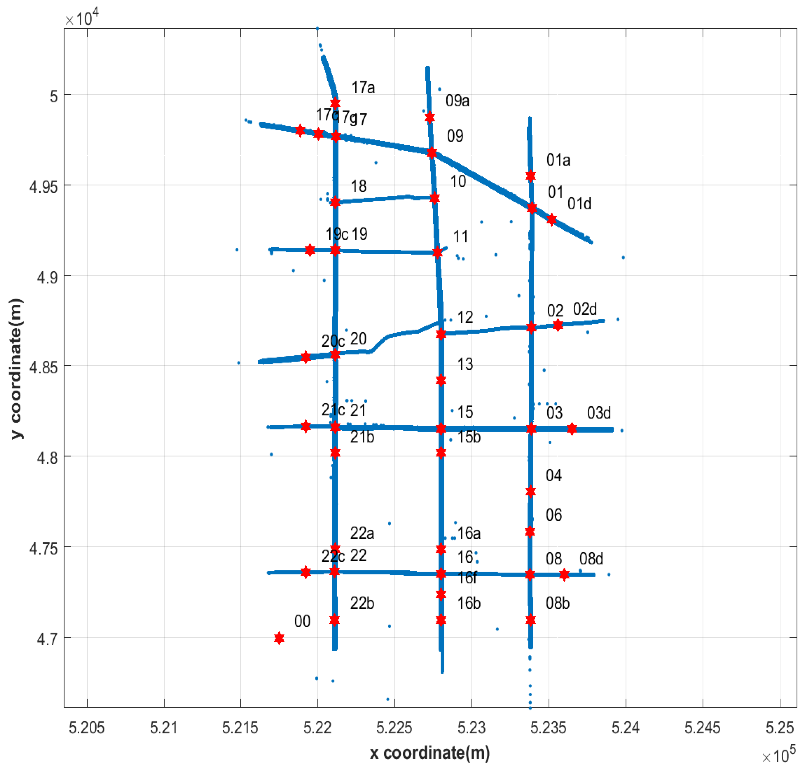
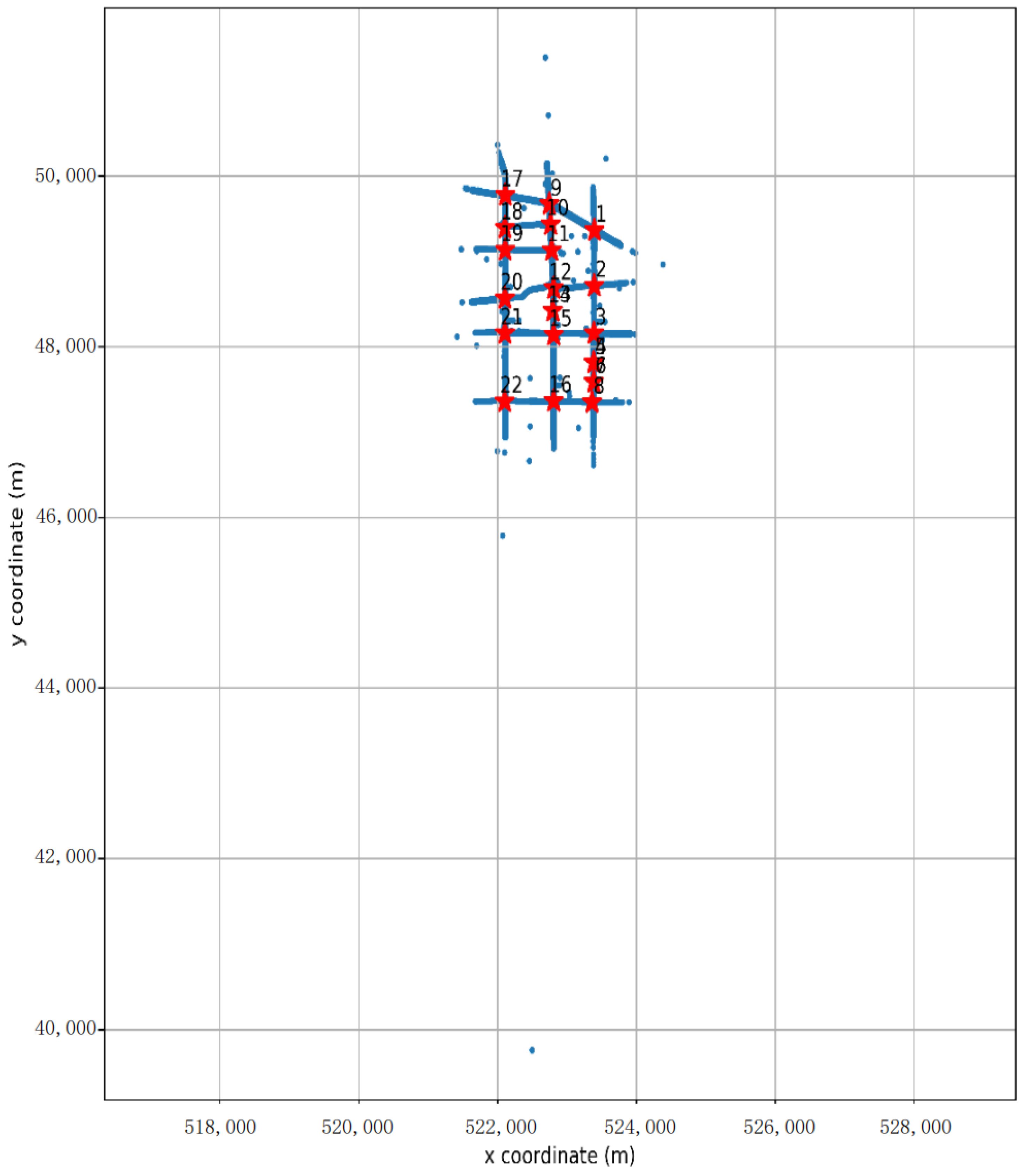
3.1.2. Spatial Coverage and Road Network Structure

The road network covered by the experimental data contains major intersections, forming a typical urban road network structure with the following characteristics:

(1)

Grid layout: Intersections exhibit a regular grid distribution, conforming to modern urban planning characteristics.

(2)

Clear hierarchy: There are distinct arterial roads (such as the arterial formed by intersections 1–8) and secondary roads.

(3)

Clear boundaries: The road network has explicit spatial boundaries, facilitating OD analysis.

(4)

Intersection coordinate data is provided in text file format, containing each intersection’s number and precise geographic coordinates. This coordinate information forms the foundation for spatial analysis and path identification.

3.1.3. Data Attributes and Quality

The trajectory data contains rich attribute information, primarily including:

(1)

Vehicle identifier (vid): Uniquely identifies each floating car

(2)

Timestamp (time): Unix timestamp format, accurate to the second

(3)

Spatial coordinates (xcoord, ycoord): Real-time vehicle position

(4)

Instantaneous speed (speed): Vehicle’s instantaneous speed in meters per second

(5)

Passenger status: Indicates whether the vehicle is carrying passengers

Regarding data quality, despite a 30.80% redundancy rate and some anomalous data, the overall quality is good and can meet analytical requirements after preprocessing. Particularly noteworthy is the high sampling frequency (primarily 3-s intervals), which ensures accurate trajectory analysis.

3.1.4. Data Representativeness and Validation

The dataset’s morning peak focus aligns with critical signal optimization needs, as this period experiences maximum traffic pressure and demonstrates the most pronounced directional flow imbalances requiring coordinated signal control. The 10 time periods (each spanning 2 h) provide sufficient temporal coverage to capture typical weekday traffic patterns while maintaining consistency. The dataset contains 7252 valid vehicles, enabling statistically reliable parameter estimation for network-level traffic analysis, though penetration rates vary across road segments. The data quality after preprocessing ensures robust parameter extraction, with successful path identification for all processed vehicles and comprehensive coverage of all major network movements.

3.2. Development Environment

This study adopts a dual-platform development strategy using Python and MATLAB, fully leveraging the advantages of both tools to construct a complete data processing and analysis system.

3.2.1. Python Development Environment

Python serves as the primary data processing platform, responsible for data preprocessing, feature engineering, and partial visualization work. The reasons for choosing Python include:

(1)

Rich data processing libraries: pandas provides powerful dataframe manipulation capabilities, numpy supports efficient numerical computation, and matplotlib and seaborn offer flexible visualization functions.

(2)

Excellent extensibility: Python’s modular design makes code easy to maintain and extend, facilitating the construction of reusable processing workflows.

(3)

Active community support: Python has widespread application in data science, making it easy to find solutions when encountering problems.

In the Python environment, this study developed a series of custom functions such as createPath(), loadData(), and dropDuplicated(). These functions encapsulate common data processing operations, improving code readability and reusability. The data storage system based on the shelve package, in particular, implements functionality similar to MATLAB’s .mat files, allowing multiple variables to be saved in a single data file, facilitating data management and sharing.

3.2.2. MATLAB Development Environment

MATLAB is primarily used for complex spatial analysis and visualization work, playing an important role particularly in intersection coordinate calibration and vehicle path identification. The reasons for choosing MATLAB include:

(1)

Powerful geometric computation capabilities: MATLAB’s built-in functions such as inpolygon() provide efficient and reliable solutions for geometric determination.

(2)

Interactive visualization: MATLAB’s graphical interface supports interactive operations such as zooming, panning, and other interactions, facilitating detailed visual analysis.

(3)

Matrix computation advantages: MATLAB excels when handling matrix operations on large-scale data.

In the MATLAB environment, core functions such as plotRoad(), selectRoad(), and routeInferMain() were developed, forming the technical foundation for path identification and parameter extraction.

3.2.3. Development Tool Integration

Data exchange between the two platforms is implemented through text files, ensuring data format compatibility. The specific workflow is as follows: Python completes data preprocessing and exports results as text files; MATLAB reads these files for further analysis; analysis results are then exported for Python to perform visualization or other processing.

While more advanced data serialization formats such as HDF5 or JSON could potentially improve I/O performance, text file exchange was selected for this study due to several practical considerations: (1) universal compatibility between Python and MATLAB environments without requiring additional libraries, (2) human-readable format facilitating debugging and data verification during algorithm development, (3) simplified data inspection and quality control processes, and (4) sufficient performance for the dataset size used in this study. For larger-scale implementations or real-time applications, more efficient serialization formats would be recommended. This loosely coupled integration approach ensures platform independence while achieving functional complementarity.

3.3. Experimental Procedure

3.3.1. Data Import and Initial Processing

The first step of the experiment is data import and format conversion. Raw data is provided in text file format and needs to be parsed and converted into structured data format. In the Python environment, data is read using pandas’ read_csv() function, followed by the following initial processing:

(1)

Data type conversion: Ensuring correct data types for each column, such as converting timestamps to integer type.

(2)

Index setting: Establishing appropriate indices to improve query efficiency.

(3)

Basic statistics: Computing basic statistical information to understand overall data characteristics.

This stage also includes creating necessary directory structures such as data/, figures/, results/, etc., preparing for subsequent processing.

3.3.2. Data Cleaning Workflow

Data cleaning is a crucial step in ensuring data quality, proceeding according to the following workflow:

(1)

Redundant data removal: Executing the dropDuplicated() function to remove duplicate records based on the combined uniqueness of vehicle ID, timestamp, and coordinates. During processing, the number of removed records is tracked in real time to assess the degree of data redundancy.

(2)

Anomalous data identification: Generating road network visualization through the plotRoadnet() function for manual identification of anomalous points obviously deviating from the road network. Based on identification results, spatial range thresholds are set for automatic anomalous data screening.

(3)

Anomalous data removal: Executing the removeOutlier() function to delete trajectory points with abnormal spatial positions and vehicles with only single trajectory points. Simultaneously, using the sortVidbyTime() function to sort vehicles by time, facilitating subsequent temporal analysis.

(4)

Data integrity check: Checking processed data for missing values and verifying data completeness.

3.3.3. Feature Engineering Implementation

Feature engineering transforms raw data into features suitable for analysis, primarily including:

(1)

Temporal feature extraction: Using the addTime() function to convert Unix timestamps to a readable time format, identifying time periods contained in the data through the timeSegment() function, and adding time period identifiers to each record using the addTimesegNo() function.

(2)

Vehicle feature construction: Generating vehicle basic feature data tables through the getVid() function, adding derived features such as time periods and start–end row numbers using the vinfoAdd() function, and constructing structured vehicle information tables to support rapid querying and analysis.

(3)

Spatial coordinate calibration: Importing processed data into the MATLAB environment, visualizing the relationship between intersection positions and trajectories using the plotRoad() function, manually adjusting intersection coordinates to trajectory convergence centers based on visualization results, and verifying calibration effects to ensure accurate positioning of all intersections.

3.3.4. Path Identification Experiment

Path identification is the core technical component of this study, with the experimental process as follows:

(1)

OD point addition: Adding original OD points at road network edges based on network topology, adding supplementary OD points for anomalous flow segments, and generating a complete node (intersection + OD point) list.

(2)

Parameter optimization experiment: Determining regular polygon radius candidate values (25 m and 49 m) based on sampling spatial distance distribution, running the path identification algorithm for each parameter setting, counting anomalous vehicle numbers, and selecting optimal parameters.

(3)

Path extraction execution:

Running the routeInferMain() main function, including the following sub-processes:

· makePolygon2(): Generating regular polygons for each node

· nodeDigger(): Determining node assignment for each trajectory point

· routeInfer(): Extracting vehicle path sequences

· routeDiagnose(): Diagnosing and processing anomalous paths

(4)

Result validation: Checking the reasonableness of path identification results, analyzing the distribution of nodes traversed by vehicles, and analyzing causes of anomalous paths. Quantitative evaluation of path inference accuracy was conducted by analyzing the proportion of successfully identified vehicle paths. With the optimal 49-m polygon radius, 7252 out of 7317 vehicles (99.1%) had their paths successfully identified, while 65 vehicles (0.9%) contained only single trajectory points and were excluded from analysis due to insufficient trajectory information for meaningful path reconstruction.

3.3.5. Traffic Parameter Calculation

Based on identified vehicle paths, various traffic parameters are calculated:

(1)

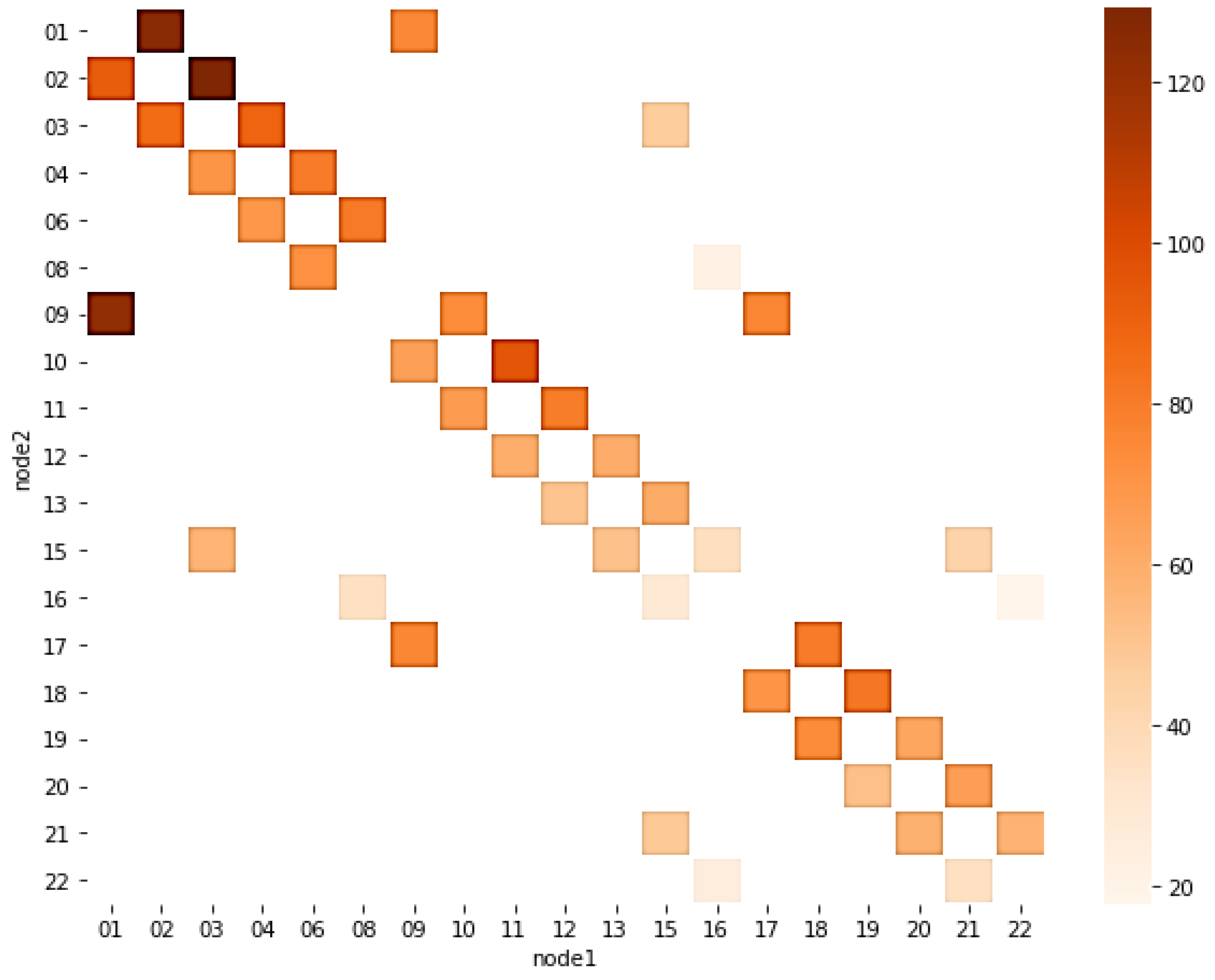
Link flow calculation: Defining the list of links to be analyzed, calling the selectVinfoMain() function with the parameter set to ‘volume’, counting vehicle numbers passing through each link in each time period, and calculating the mean and standard deviation of flow.

(2)

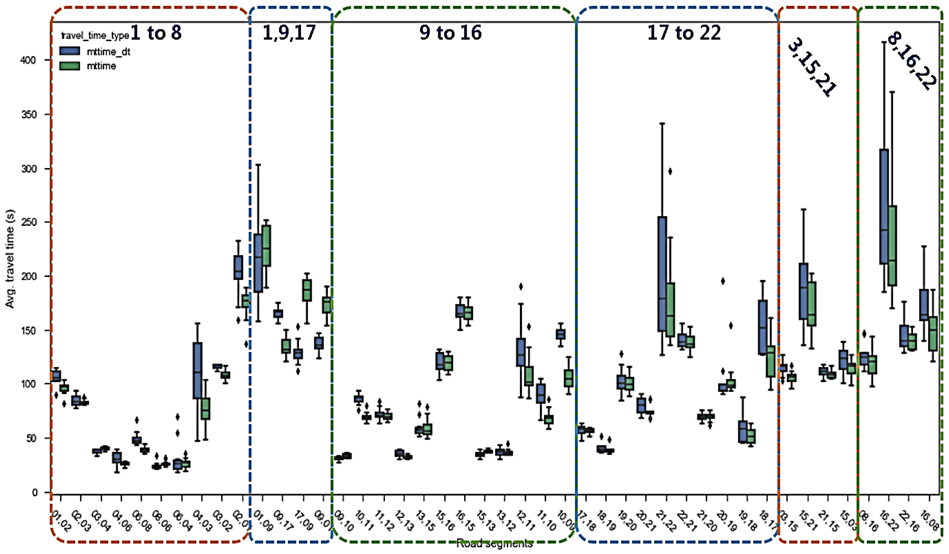
Speed and travel time calculation: Using dual calculation methods (based on instantaneous speed and time difference), extracting speed and time parameters simultaneously through the selectVinfoMain() function, fusing results from both methods to improve estimation accuracy.

(3)

Approach flow analysis: Identifying turning relationships at each intersection, calculating left-turn flow using the tpVolume3() function, and generating intersection-level flow statistics tables.

(4)

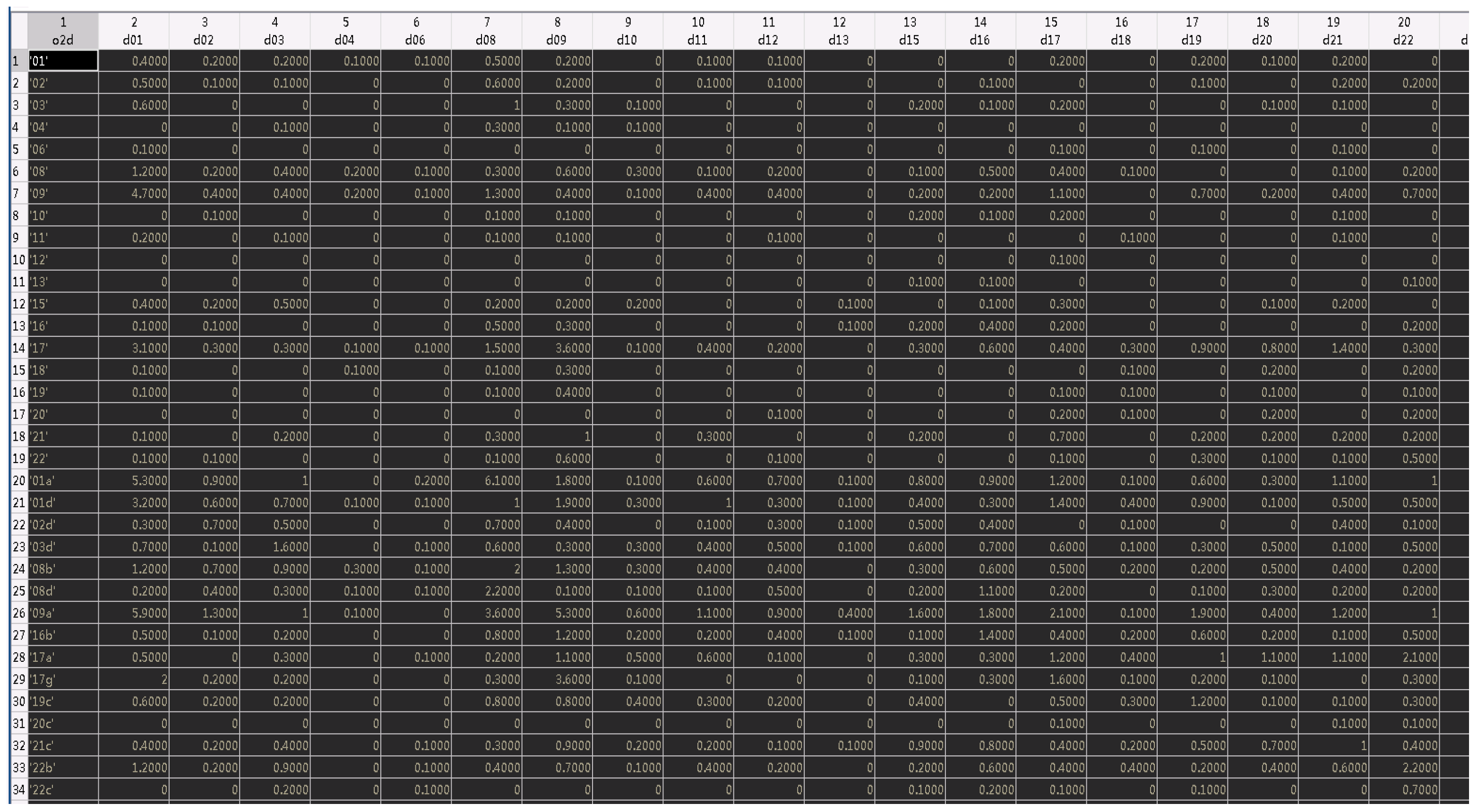
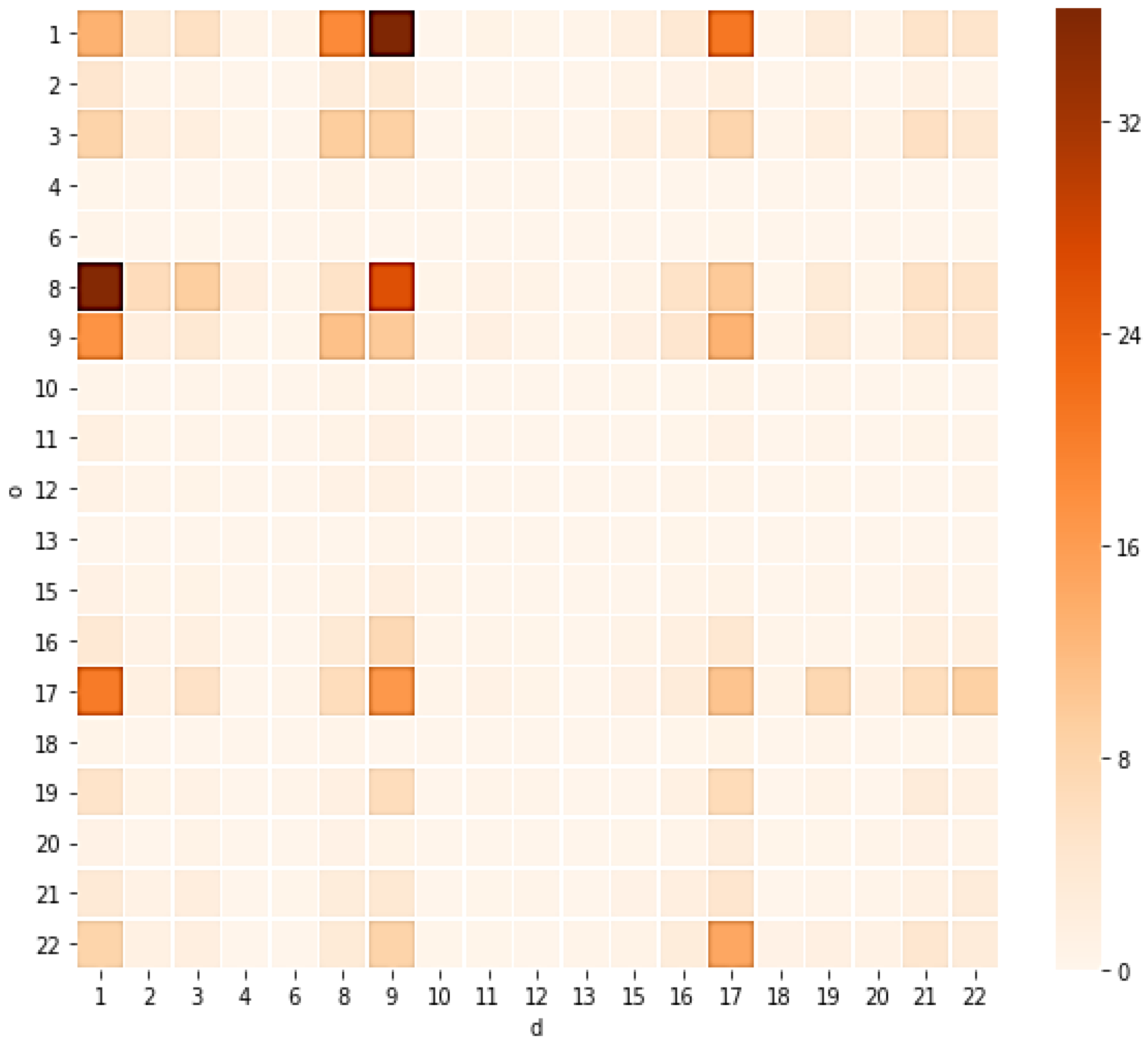
OD matrix construction: Counting OD pairs based on vehicle path data, generating both basic and detailed OD matrices, and calculating time period averages of OD flows.

3.3.6. Result Visualization

Visualization is an important means for understanding and presenting analysis results:

(1)

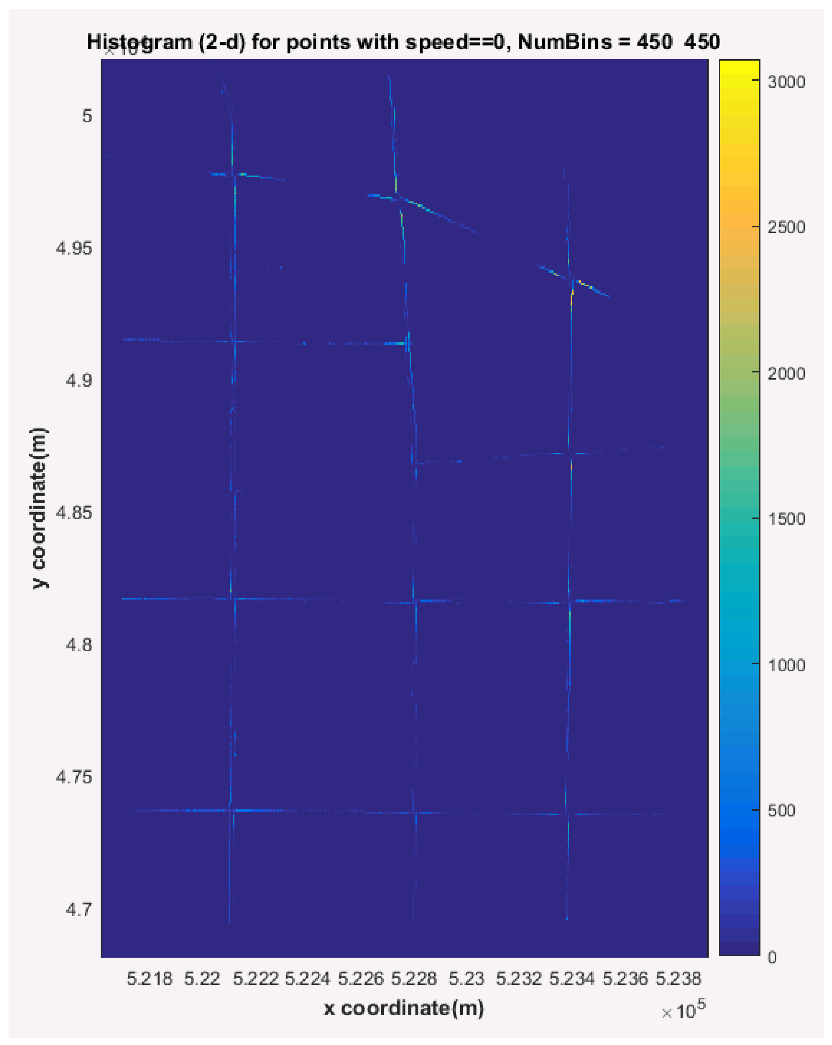
Stop point density visualization: Extracting trajectory points with zero speed, using 2D histograms to analyze spatial distribution, and generating heat maps to display congestion distribution.

(2)

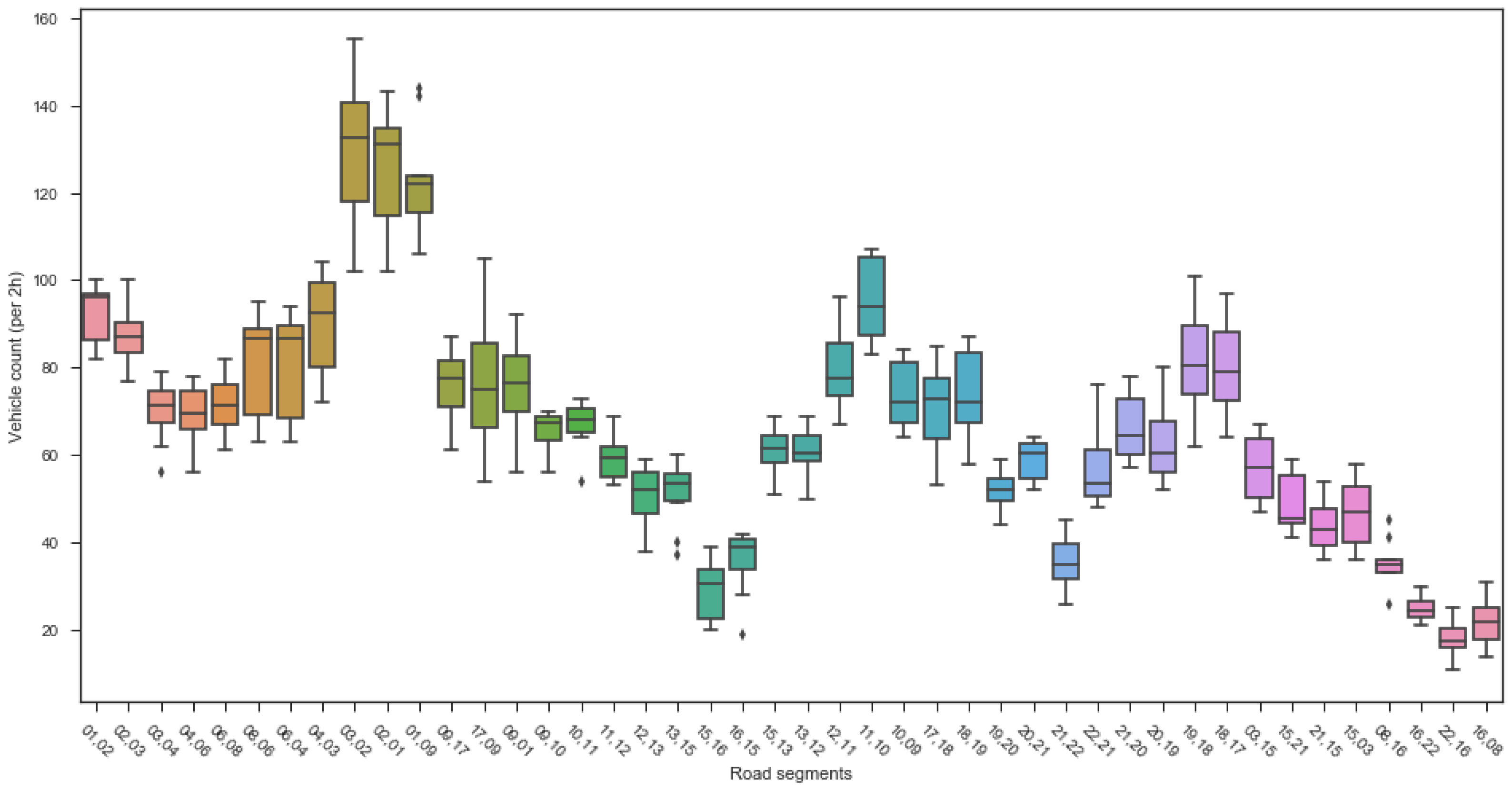
Traffic parameter visualization: Using box plots to display distributions of speed, travel time, and flow, generating time series plots to show temporal variation characteristics of parameters, and creating spatial distribution maps to show spatial differences in parameters.

(3)

Comprehensive analysis charts: OD matrix heat maps, road network flow distribution maps, and key indicator comparison charts.

3.4. Experimental Parameter Setting and Optimization

Key parameter settings in the experiment have a significant impact on results. This study ensures method effectiveness through systematic parameter optimization.

3.4.1. Spatial Parameter Settings

(1)

Regular polygon sides: Selecting hexadecagons as the shape for node coverage areas. This choice is based on the following considerations: too few sides (e.g., quadrilaterals) result in significant differences between coverage areas and actual road shapes; too many sides increase computational complexity with limited accuracy improvement. Hexadecagons achieve a good balance between accuracy and efficiency.

(2)

Circumscribed circle radius: The polygon radius selection was based on analysis of the spatial sampling characteristics of the trajectory data. Specifically, sampling spatial distances (excluding zero distances and sampling intervals ≥5 s) were analyzed, and the 99th percentile distance was calculated as 49 m. The second candidate radius of 25 m represents half of the 99th percentile value, allowing comparison of algorithm performance under different coverage scales to determine the optimal parameter setting.

(3)

Anomalous data threshold: Based on road network visualization results, setting determination thresholds for abnormal spatial positions to ensure removal of trajectory points obviously deviating from the road network while retaining normal data in edge areas.

3.4.2. Temporal Parameter Settings

(1)

Time window division: Each time period is set to 2 h, matching the actual morning peak duration, ensuring sufficient data volume while avoiding confusion from cross-period traffic patterns.

(2)

Sampling interval threshold: When analyzing sampling characteristics, sampling time intervals are divided into two categories: less than 10 s and greater than or equal to 10 s. This threshold selection is based on data distribution characteristics and can effectively distinguish normal sampling from anomalous intervals.

3.4.3. Algorithm Parameter Optimization

(1)

Data storage format: Providing two storage options, ‘manytable’ and ‘onetable’, where the former is suitable for detailed segment-by-segment analysis and the latter facilitates overall comparison and statistics.

(2)

Parallel processing settings: When processing large-scale data, reasonably setting the number of parallel processing threads to balance computational resources and processing efficiency.

(3)

Visualization parameters: Including histogram bin numbers, chart color schemes, and annotation detail levels. These parameter settings must ensure sufficient information display while avoiding visual clutter.

4. Experimental Results and Analysis

4.1. Traffic Parameter Extraction Results

Based on the identified vehicle trajectories, this study extracted multi-dimensional traffic parameters that comprehensively characterize the operational state of the road network.

4.1.1. Link Flow Characteristics

Link flow serves as a fundamental indicator reflecting road utilization intensity. By calculating the number of vehicles passing through each link during different time periods, the flow distribution characteristics of the road network were obtained.

According to the flow box plot analysis in Figure 6, the flow distribution in the road network exhibits distinct hierarchical characteristics. Major arterials, particularly the north–south arterial formed by intersections 1–8 and the east–west arterial formed by intersections 1, 9, and 17, carry the predominant traffic flow in the network. These links demonstrate significantly higher average flows compared to other segments, with relatively stable flow variations (indicated by smaller box sizes).

Secondary links exhibit notably lower flows with varying degrees of volatility. Some secondary links maintain stable but low flows, likely serving localized traffic demands, while others display higher flow fluctuations, potentially influenced by specific time periods or special events. This differentiated flow distribution provides a basis for differential signal timing design: major links should receive longer green times and better coordination control, while secondary links can adopt shorter cycles to minimize delays.

Temporal stability of flows is reflected through the dispersion of data across different time periods. Most links exhibit relatively small flow standard deviations, indicating good regularity in weekday morning peak traffic demands. This regularity constitutes an important prerequisite for implementing fixed-time signal control.

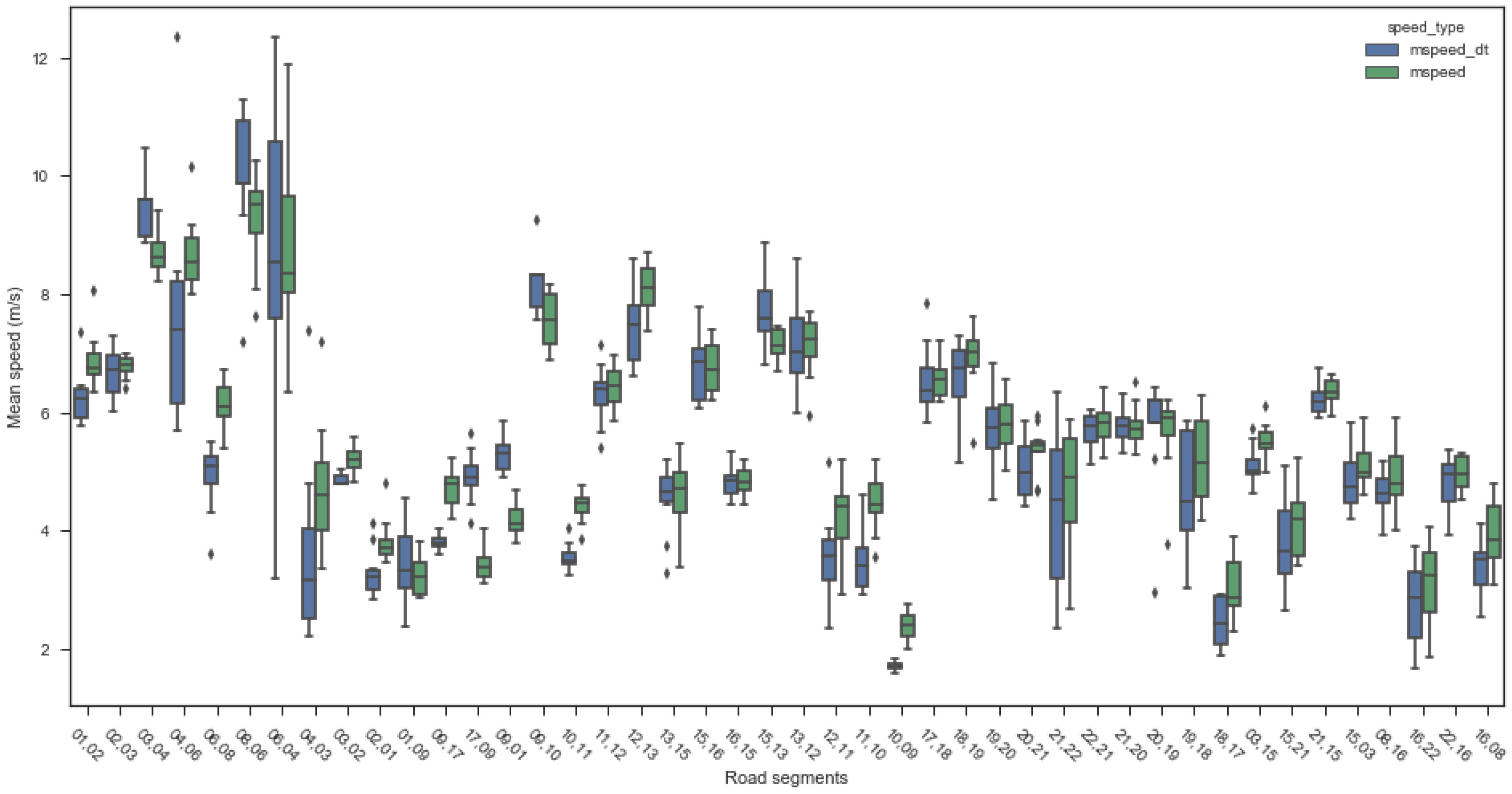
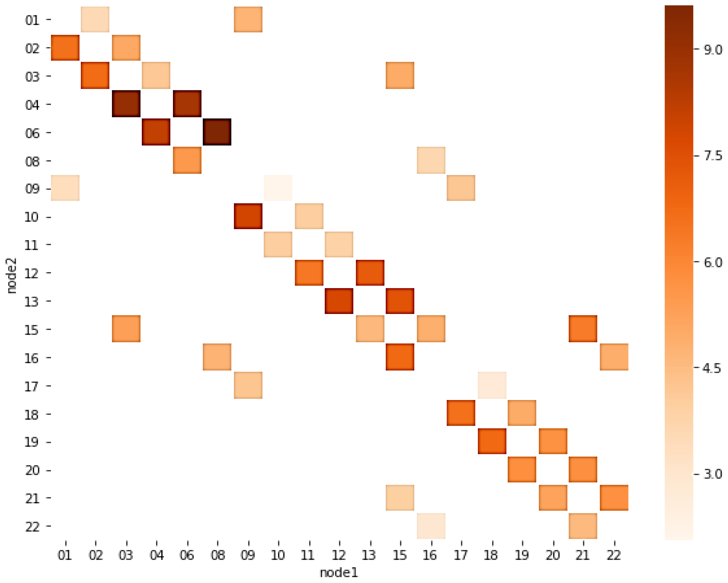
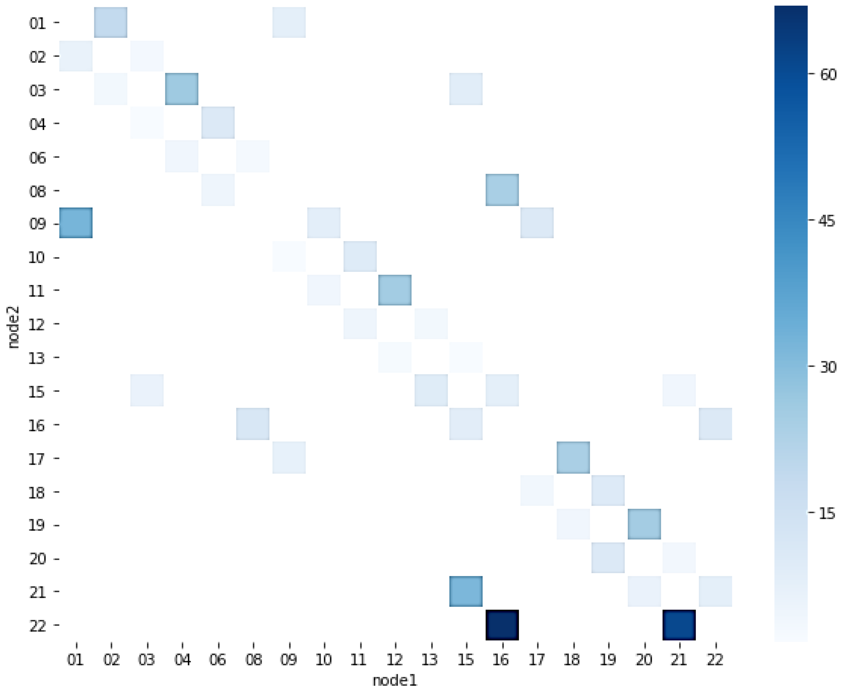
4.1.2. Link Average Speed

Speed represents a core indicator for evaluating traffic operational efficiency. The dual calculation method employed in this study provides more reliable speed estimates, with specific results shown in Figure 7.

The spatial heterogeneity of speed distribution is pronounced. Certain links, such as those between intersections 4 and 6, exhibit extreme speed fluctuations, with box plots revealing numerous outliers. Further analysis suggests these links may experience severe stop-and-go phenomena: free-flow conditions with high speeds during some periods, contrasted with severe congestion and near-zero speeds during others. This unstable traffic state poses challenges for signal control, potentially necessitating adaptive control strategies.

Links ‘21,22’ and ‘16,22’ also demonstrate substantial speed variations, albeit with slightly different patterns. The speed distributions for these links exhibit multimodal characteristics, potentially reflecting the coexistence of different traffic states: free-flow and congested conditions alternating across different time periods. This characteristic suggests these links may represent sensitive areas for traffic state transitions, requiring special attention in signal control design.

The two speed calculation methods (instantaneous speed-based mspeed and time difference-based mspeed_dt) yield generally consistent results, though systematic differences exist on certain links. These differences likely stem from the inherent characteristics of each method: the instantaneous speed approach is more sensitive to localized speed variations, while the time difference method provides link-level average effects. By fusing results from both methods, the robustness of speed estimation is enhanced.

4.1.3. Average Travel Time

Travel time represents the most directly perceived level-of-service indicator for travelers and serves as a key input parameter for signal coordination control. Figure 8 illustrates the distribution characteristics of travel times across various links:

Travel time variability correlates highly with speed fluctuations yet exhibits distinct characteristics. Links ‘4,3’, ‘1,9’, ‘21,22’, and ‘16,22’ display substantial travel time variations. These fluctuations not only reflect traffic state instability but may also relate to signal control discoordination. Particularly for link ‘1,9’, as part of a major arterial, its high travel time variability may severely impact arterial coordination effectiveness.

The distribution patterns of travel times provide additional insights. Several links exhibit pronounced right-skewed travel time distributions, characterized by a small number of extreme values. These extreme values typically correspond to travel times under severe congestion conditions, and while their occurrence frequency may be low, their impact on user experience is substantial. Signal optimization should consider not only minimizing average travel times but also performance under extreme conditions.

Travel times calculated using both instantaneous speed and time difference methods (mttime and mttime_dt) demonstrate good consistency across most links, validating the reliability of the calculation approaches. However, substantial differences between methods exist on certain specific links, typically areas with complex traffic states or data quality issues, requiring special attention in practical applications.

4.1.4. OD Matrix Analysis

The OD matrix comprehensively reflects travel demand distribution within the road network, serving as fundamental data for traffic planning and management. The two types of OD matrices generated in this study provide information at different levels:

The basic OD matrix (19 × 20 dimensions) focuses on flow exchanges between intersections. As shown in Figure 9, OD flow distribution is highly uneven, with several dominant OD pairs. These high-flow OD pairs typically correspond to important commuting corridors or connections between commercial and residential areas. The basic OD matrix (19×20 dimensions) clearly demonstrates that OD flow distribution is highly uneven, with several dominant OD pairs constituting the primary traffic flows within the network. These high-flow corridors typically represent important commuting routes, with intersections 1, 9, and 17 serving as major traffic generation and attraction points that maintain strong connections with multiple other intersections. Identifying these key OD pairs holds significant importance for arterial coordination control design: green wave coordination should be prioritized for high-flow OD pairs.

The detailed OD matrix incorporates OD point information, providing finer-grained origin–destination distributions. As partially shown in Figure 10, OD points at the network periphery handle substantial collection and distribution functions. This finding validates the necessity of adding OD points while also suggesting the need to consider special requirements of traffic entering and exiting the network in signal control design. The detailed OD matrix incorporates peripheral OD point information, revealing that boundary OD points handle substantial traffic collection and distribution functions. This finer-grained analysis provides essential input for designing signal coordination strategies that accommodate both internal circulation patterns and external access requirements at network entry/exit points.

Notably, the OD matrix contains a certain amount of same-point OD flows (identical origins and destinations). As mentioned earlier, the average flow from intersection 1 to intersection 1 reaches 13.1 vehicles. This phenomenon may have multiple explanations: vehicles conducting short-distance activities near the node before returning, data recording start and end times coincidentally falling within the node’s range, or taxi cruising behavior in the area. Such special travel patterns require particular consideration in signal control optimization.

4.2. Visualization Analysis

Data visualization transforms abstract numbers into intuitive graphics, facilitating the discovery of hidden patterns and regularities within the data.

4.2.1. Stop Point Density Analysis

Stop point density maps intuitively illustrate congestion distribution across the road network. Through spatial density analysis of trajectory points with zero speed, significant analytical results were obtained.

According to the overall density distribution in Figure 11, congestion in the road network exhibits distinct spatial clustering characteristics. Intersections 1, 2, 3, 9, and 17 form several prominent high-density centers, representing critical nodes within the network. High stopping densities not only indicate frequent vehicle stops but may also lead to queue spillback, affecting normal operations at upstream intersections.

Examining specific intersection levels reveals more detailed congestion characteristics. Congestion at intersection 1 primarily concentrates in the northbound direction, with stop point density maps indicating severe queuing in this direction. Similarly, the northbound approach at intersection 2 also exhibits high-density characteristics. This directional congestion distribution closely correlates with morning peak commuting patterns: substantial vehicular flow from southern residential areas toward northern commercial districts.

Intersections 9 and 17 display relatively uniform stop density distributions, with congestion present to varying degrees in all directions. This likely results from their strategic positions within the network, handling multi-directional traffic conversion functions. For such intersections, balanced consideration across all approaches is necessary to avoid favoring one direction at the expense of others.

Analysis of the intersection cluster comprising nodes 15, 16, 21, and 22 reveals another congestion pattern: stop densities at north–south approaches significantly exceed those at east–west approaches. This may relate to the area’s road network structure and land use layout. Signal optimization should allocate more green time to north–south movements.

4.2.2. Link Traffic Flow Direction Characteristic Analysis

To thoroughly understand directional characteristics of traffic flow, this study conducted a comparative analysis of traffic parameters for different flow directions on each link. By analyzing bidirectional average speeds, travel times, and flow distributions for each link, tidal traffic characteristics during morning peak periods can be accurately identified.

The distribution of average speeds by direction for each link (Figure 12) clearly demonstrates directional speed disparities. On most links, reverse direction speeds (westbound and southbound) significantly exceed forward direction speeds, consistent with the dominant flow from residential areas to employment centers during morning peak periods. This speed advantage is particularly pronounced on reverse direction links such as 8–1, 16–9, and 22–17, indicating relatively lower traffic pressure and underutilized road capacity in these directions.

The distribution of average travel times by direction for each link (Figure 13) validates the tidal phenomenon from another perspective. Forward direction links generally exhibit longer travel times with greater variation ranges, reflecting congestion severity and instability. In contrast, reverse direction links demonstrate shorter and relatively stable travel times. This disparity provides justification for implementing asymmetric signal control strategies.

The distribution of average flows by direction for each link (Figure 14) directly reflects directional imbalance in traffic demand. Forward flows significantly exceed reverse flows, with differences reaching 2–3 times on certain links. This flow distribution imbalance serves as an important basis for determining split allocations, with green times for each direction adjusted according to actual flow proportions.

Based on flow direction characteristic analysis, signal control optimization should adopt the following strategies: First, implement asymmetric green wave control, providing wider bandwidth for dominant flow directions; second, dynamically adjust splits, allocating green times according to real-time flow proportions; third, consider traffic space optimization measures such as reversible lanes to improve road resource utilization efficiency.

4.2.3. OD Distribution Visualization Analysis

The Origin–Destination (OD) matrix serves as an important tool for understanding the spatial distribution of traffic demand. Through visualization analysis of the extracted OD matrix, major traffic flows and key OD pairs can be identified.

The vehicle OD distribution diagram (Figure 15) employs a heat map format to display OD flows between intersections. Several characteristics are clearly evident from the diagram: First, OD distribution exhibits pronounced asymmetry, reflecting directional traffic flow characteristics during morning peak periods; second, several high-flow OD pairs exist, constituting the primary traffic flows within the network; finally, certain intersections (such as 1, 9, and 17) serve as major traffic generation or attraction points, maintaining strong connections with multiple other intersections.

Spatial pattern analysis of OD distribution reveals the functional structure of the road network. Peripheral intersections (such as 1, 2, and 3) primarily function as traffic generation points, channeling traffic flow toward inner intersections; central area intersections (such as 9, 10, and 11) mainly serve as traffic attraction points, receiving traffic flows from various directions. This “periphery-to-center” OD pattern represents typical centripetal commuting traffic characteristics.

Based on OD distribution characteristics, signal control optimization should focus on paths of high-flow OD pairs. Through path analysis, identify the primary travel routes of these OD pairs, ensuring signal coordination along these paths to reduce stops and delays. Meanwhile, for lower-flow OD pairs, their operational efficiency can be appropriately sacrificed to ensure the smooth flow of major traffic streams.

4.2.4. Traffic Parameter Volatility Analysis

Traffic parameter volatility reflects traffic flow stability and serves as an important indicator for assessing link operational reliability. This study analyzed traffic parameter fluctuation characteristics by calculating standard deviations of average speeds and travel times for each link.

The variance distribution of average speeds for each link (Figure 16) reveals spatial heterogeneity in speed fluctuations. Certain links exhibit significantly higher speed variances than others, indicating extremely unstable traffic conditions on these segments. High-volatility links often represent traffic bottlenecks, prone to cycles of congestion formation and dissipation. This instability imposes higher requirements on signal control, necessitating greater safety margins.

The variance distribution of average travel times for each link (Figure 17) further confirms traffic flow instability. Links with high travel time variance largely coincide with those exhibiting high speed variance, forming “vulnerable segments” within the network. These links are sensitive to external disturbances, where minor perturbations may lead to substantial delay increases.

Volatility analysis results provide important guidance for signal control optimization. For high-volatility links, the following measures should be adopted: First, consider volatility in offset calculations, using mean values plus a certain proportion of standard deviation to determine offsets; second, implement adaptive control strategies, dynamically adjusting signal timing based on real-time traffic conditions; third, strengthen traffic flow stability management, reducing inflow fluctuations through measures such as upstream metering control.

The average travel time diagram for each link (Figure 18) comprehensively illustrates the overall operational status of the road network. The diagram shows that the spatial distribution of travel times highly correlates with indicators such as stop density and speed fluctuations, validating the consistency of multi-dimensional parameter analysis. Links with longer travel times primarily concentrate along several key corridors, which should serve as priority areas for signal optimization.

Through the above multi-perspective visualization analysis, this paper has comprehensively grasped the traffic operational characteristics of the road network. Stop density analysis identified congestion hotspots, flow parameter box plots revealed parameter distribution characteristics, flow direction characteristic analysis discovered tidal traffic patterns, OD distribution analysis clarified major traffic demands, and volatility analysis assessed operational reliability. These visualization results mutually validate and complement each other, collectively forming the data foundation for signal control optimization. Based on these analytical results, targeted optimization strategies can be formulated, including coordination control subarea division, offset optimization, split adjustment, and oversaturation control, ultimately achieving overall improvement in network operational efficiency.

5. Guidance of Traffic Parameters for Signal Control Optimization

Traffic parameters extracted from vehicle trajectory data provide multi-dimensional and refined data support for traffic signal control optimization. Compared with traditional fixed detector-based data, the rich information contained in trajectory data can more comprehensively reflect traffic flow operational states, providing a scientific basis for formulating and optimizing signal control strategies. This section presents an in-depth analysis from multiple dimensions on how extracted traffic parameters guide and support signal control optimization.

5.1. Guidance for Coordination Control Subarea Division

Regional coordination control represents an important approach for improving overall network operational efficiency, while the scientific division of coordination control subareas constitutes a prerequisite for achieving effective coordination. Multi-dimensional traffic parameters extracted from trajectory data provide a quantitative basis for subarea division.

Through a comprehensive analysis of parameters including link flows, intersection spacing, average travel times, and vehicle OD volumes between intersections, traffic correlation between intersections can be accurately quantified. When flow from an upstream node into a downstream node approaches or exceeds the downstream node’s approach capacity, greater flows or larger ratios of average queue length at the downstream node approach to link length between upstream and downstream nodes indicate a stronger correlation between the two nodes. Additionally, more OD paths passing through two nodes and greater OD path flows also strengthen inter-node correlation.

Based on the above principles and combined with extracted traffic parameter analysis, the study network can be divided into four coordination control subareas:

(1)

Intersections 1, 9, 17 subarea: forming an east–west arterial coordination system

(2)

Intersections 2–8 subarea: constituting a north–south major arterial coordination system

(3)

Intersections 10–16 subarea: covering the central area network

(4)

Intersections 18–22 subarea: controlling peripheral area traffic flows

This subarea division method, based on actual traffic flow characteristics, compared with traditional methods based on geometric distance or administrative boundaries, better reflects inherent traffic flow relationships and helps improve coordination control effectiveness. Particularly during morning peak periods, this division can effectively address the special requirements of tidal traffic flows.

5.2. Decision Support for Offset Optimization

Offset constitutes the core parameter for arterial coordination control, directly affecting green wave bandwidth and coordination effectiveness. Link average travel times and average speeds extracted from trajectory data provide precise data foundation for offset calculation and optimization.

Traditional offset calculation typically assumes constant vehicle speeds, while actual traffic flow speeds exhibit significant spatiotemporal variations. By analyzing travel time distribution characteristics across different time periods and links, a more refined offset design can be achieved:

(1)

Basic offset determination: Calculate typical travel times between adjacent intersections based on link average travel times. For instance, if a link’s average travel time is 45 s, the basic offset should be set as an integer multiple of 45 s to ensure vehicles can pass through downstream intersections during green phases.

(2)

Dynamic adjustment strategy: For links with high speed fluctuations (such as link ‘4,6’ and links ‘21,22’ and ‘16,22’ in the experimental results), offsets need fine-tuning based on speed distribution standard deviations. When standard deviations are large, safety margins for offsets should be appropriately increased to prevent vehicles from missing green phases due to speed fluctuations.

(3)

Tidal phenomenon response: Pronounced directional imbalances exist during morning peak periods. Through analyzing bidirectional flow ratios and speed differences, offsets can be optimized accordingly. Experimental data indicates that directions 8–1, 16–9, and 22–17 (reverse green waves) carry substantial flows during morning peaks, warranting increased green wave bandwidth in these directions with corresponding offset adjustments to match actual demands.

(4)

Multi-path coordination: Based on OD matrix analysis, identify primary traffic flow paths and ensure offset settings along critical paths can form continuous green wave effects. This multi-path offset optimization approach can enhance overall network operational efficiency.

5.3. Oversaturation State Identification and Control

Oversaturation states during morning peak periods represent challenging aspects of urban traffic management, with traditional control methods often proving ineffective. Parameter extraction based on trajectory data provides new approaches for identifying and controlling oversaturation states.

Multi-dimensional identification of oversaturation states:

(1)

Stop point density identification: Through analyzing the spatial distribution of vehicle stop points, congestion hotspots can be intuitively identified. Experimental results indicate that intersections 1, 2, 3, 9, and 17 exhibit significantly higher stop densities than other areas, with the northbound approaches at intersections 1 and 2 being most severe.

(2)

Travel time volatility analysis: Standard deviations of link travel times reflect traffic flow stability. Large standard deviations indicate that links are prone to cycles of congestion formation and dissipation, representing potential bottleneck segments.

(3)

Queue length estimation: Based on stop point density and vehicle trajectories, queue lengths at various approaches can be estimated. When queue lengths approach link lengths, queue spillback risks exist.

Secondary congestion prevention strategies: Under oversaturated conditions, excessive intersection queues easily lead to secondary congestion, disrupting original coordination control effects. Preventive measures are therefore necessary:

(1)

Travel time reduction: In offset optimization, apply travel time reductions for links prone to queue spillback, reserving buffer space to absorb queue fluctuations.

(2)

Gating control: When links experience oversaturation, appropriately shorten green times for traffic entering the area, preventing or gating large vehicle volumes from entering to avoid regional gridlock.

(3)

Evacuation priority: Appropriately extend green times at congested area exits to accelerate vehicle evacuation from the area, alleviating internal congestion.

5.4. Signal Control Scheme Evaluation System

Extracted multi-dimensional traffic parameters not only provide inputs for signal control optimization but also constitute a comprehensive effectiveness evaluation system. This evaluation method, based on actual operational data, proves more objective and accurate compared with traditional simulation evaluation.

Multi-level evaluation indicator system:

(1)

Microscopic level: Vehicle-level indicators including number of stops, travel times, and speed fluctuations, reflecting individual travel experiences

(2)

Mesoscopic level: Link average speeds, flows, densities, and other indicators, evaluating link operational efficiency

(3)

Macroscopic level: Network average speeds, total delays, system throughput, and other indicators, measuring overall performance

Furthermore, parameter extraction based on trajectory data possesses near-real-time characteristics, enabling dynamic monitoring and feedback, specifically including: continuous monitoring of signal control effectiveness, timely detection of abnormal states, dynamic adjustment of control schemes, and long-term trend analysis and evaluation.

5.5. Data Support for Intelligent Control Algorithms

With the development of artificial intelligence technology, data-driven intelligent signal control has become a development trend. Rich parameters extracted from trajectory data provide high-quality inputs for intelligent control algorithms, specifically including:

(1)

Feature engineering for machine learning models: Extracted parameters including link flows, speeds, densities, and travel times can directly serve as feature inputs for machine learning models. Compared with traditional single-flow data, multi-dimensional features can more comprehensively describe traffic states, improving model prediction accuracy and generalization capability. Features include:

• Temporal features: Flow and speed variations across different time periods
• Spatial features: Correlation parameters of upstream and downstream links
• State features: Indicators reflecting saturation levels such as density and queue lengths

(2)

Application of Bayesian optimization: Average travel time parameters can be combined with Gaussian process-based Bayesian optimization methods to achieve intelligent offset optimization. Advantages of Bayesian optimization include:

• Capability to handle nonlinear and non-convex optimization problems
• High sample efficiency, suitable for computationally expensive scenarios
• Ability to quantify uncertainty, providing robust optimization results

(3)

State space for reinforcement learning: For more complex adaptive signal control, extracted traffic parameters can constitute the state space for reinforcement learning:

• Current state: Real-time density, speed, and queue lengths for each link
• Historical state: Parameter change trends over the past several cycles
• Predicted state: Future flow predictions based on OD matrices

This rich state representation can help agents learn superior control strategies, achieving proactive traffic control adaptable to demand changes.

In summary, traffic parameters extracted from vehicle trajectory data provide comprehensive data support for signal control optimization. From coordination control subarea division to specific offsets, from oversaturation state identification to intelligent control algorithm applications, these parameters play important roles in all aspects of signal control. Compared with traditional fixed detector-based methods, trajectory data not only provides equivalent information but also reveals spatiotemporal evolution patterns of traffic flows, providing a solid data foundation for achieving more intelligent and efficient signal control.

6. Conclusions and Future Directions

6.1. Main Conclusions

Main Research Objectives: (1) Develop a systematic trajectory data processing framework ensuring consistent data quality; (2) create an innovative trajectory point-labeling algorithm for accurate road network mapping; (3) establish multi-source data fusion methods to improve parameter estimation reliability; (4) build automated and reusable processing tools for practical engineering applications; (5) validate methodology effectiveness using large-scale real-world trajectory data.

This research addresses challenges faced by traditional traffic parameter acquisition methods, including poor data quality and acquisition difficulties, by proposing a comprehensive method for traffic parameter extraction and analysis based on vehicle trajectory data. Through theoretical innovation and engineering practice, the following main achievements and conclusions were obtained:

6.1.1. Method Effectiveness Validated

Through processing and analyzing actual trajectory data containing over 2.48 million records, the effectiveness of the proposed method was validated. The data preprocessing phase successfully eliminated 30.80% of redundant data, improving data quality. This result not only demonstrates the necessity of systematic data cleaning but also provides a quantitative reference for trajectory data quality control.

The path identification algorithm successfully processed trajectory data from 7252 vehicles, accurately identifying node sequences traversed by vehicles. Through parameter optimization, 49 m was determined as the optimal radius for polygon circumscribed circles, with this setting yielding the minimum number of abnormal vehicles and optimal path identification results. This achievement indicates that parameter optimization based on data characteristics is key to improving algorithm performance.

The research contributes to scientific knowledge through (1) the novel regular polygon coverage algorithm that solves trajectory point-labeling challenges more effectively than traditional nearest-neighbor approaches; (2) the systematic five-module processing framework addressing fragmentation in existing research; (3) the multi-source data fusion approach combining instantaneous speed and time difference calculations for enhanced reliability; and (4) the highly automated toolchain enabling practical engineering applications. Social implications include providing cost-effective alternatives for regions lacking traditional detection infrastructure, supporting intelligent traffic management through comprehensive parameter extraction, and facilitating data-driven traffic control optimization that can reduce congestion and improve urban mobility.

Traffic parameter extraction covered multiple dimensions, including link flows, average speeds, travel times, and OD matrices. These parameters were not only complete in quantity but also ensured accuracy through multi-source fusion calculations.

6.1.2. Technical Innovations Hold Significant Value

This study achieved technical innovations in multiple aspects, which not only solved specific technical problems but also provided new perspectives for related field development:

The trajectory point-labeling algorithm based on polygon coverage represents an innovation of this paper. This algorithm cleverly transforms the continuous trajectory discretization problem into geometric containment relationship determination, improving computational efficiency while ensuring identification accuracy. Compared with traditional map-matching algorithms, this method does not require detailed road network topology information, lowering application barriers. The algorithm demonstrates good interpretability and stability, performing excellently in practical engineering applications.

The systematic methodological framework represents another innovation. This study proposes, for the first time, a complete parameter extraction process oriented toward signal control optimization, from data preprocessing to feature extraction, from microscopic trajectories to macroscopic parameters, with each step carefully designed. This solution avoids disconnection between different processing stages, improving overall efficiency. The framework’s modular design provides good scalability, easily adapting to different application requirements.

The concept of multi-source data fusion permeates the entire study. Employing multiple methods in parameter calculation and fusing results not only improves estimation accuracy but also provides inherent quality control mechanisms. This concept has universal significance and can be extended to other types of traffic data analysis.

6.1.3. Parameter Extraction Results Accurately Reflect Network State

Extracted traffic parameters comprehensively reflect the operational state of the road network, providing a reliable data foundation for signal control optimization:

Flow analysis revealed the primary–secondary structure of the road network. Major arterials (formed by intersections 1–8 and 1, 9, 17) carry primary traffic flows with relatively stable volumes; secondary links have smaller flows but varying volatility. This differentiated flow distribution provides a basis for differential signal timing design.

Speed and travel time analysis identified unstable links. Links ‘4,6’, ‘21,22’, ‘16,22’ and others exhibited substantial speed fluctuations and travel time variability, suggesting these links may experience severe traffic state transitions requiring special attention in signal control.

Stop point density analysis intuitively illustrates congestion distribution. Intersections 1, 2, 3, 9, and 17 were identified as congestion hotspots, exhibiting pronounced directional characteristics (such as severe northbound approach congestion at intersections 1 and 2). These findings align with morning peak commuting patterns, validating the reasonableness of analysis results.

OD matrices provided demand distribution information. Identifying major OD pairs and high-flow corridors provides important inputs for network-level signal coordination. Additionally, edge OD point information contained in detailed OD matrices helps understand network collection and distribution characteristics.

6.1.4. Practical Value Fully Demonstrated

This study not only achieves theoretical innovation but, more importantly, demonstrates significant practical value:

It provides feasible technical solutions for regions lacking traditional detection equipment. With the development of new transportation modes such as connected vehicles, ride-hailing vehicles, and shared vehicles, trajectory data acquisition becomes increasingly accessible, and this method can precisely utilize such data to extract traffic parameters, avoiding expensive detection equipment investments.

The developed toolchain features high reusability and automation. The dual-platform implementation based on Python and MATLAB combines the advantages of both tools. Detailed code comments, standardized interface design, and flexible parameter configuration enable convenient method portability to other projects.

Extracted parameters can be directly applied to signal control optimization. Parameter types, granularity, and accuracy all meet practical signal control requirements, serving as inputs for various optimization algorithms. This practicality represents an important design objective and a direct manifestation of the method’s value.

6.1.5. Research Limitations and Assumptions

Several limitations and assumptions should be acknowledged in this study. The methodology’s effectiveness depends on trajectory data quality and sampling frequency, with validation conducted using predominant 3-s intervals that may not represent all data collection scenarios. The regular polygon coverage algorithm assumes vehicles follow relatively predictable paths near intersections, which may not hold during unusual traffic events or in complex network configurations. The approach assumes sufficient vehicle penetration rates across road segments, though actual penetration rates remain unknown and may affect parameter accuracy in low-traffic areas. Additionally, the intersection coordinate calibration currently requires manual adjustment, limiting fully automated deployment. While demonstrated effectiveness on a grid-like urban network, performance may vary with irregular network layouts or in different geographical contexts. These limitations suggest that careful consideration of local conditions and data characteristics is essential for successful implementation in diverse operational environments.

6.2. Future Directions

Based on this study’s achievements and identified issues, the following suggestions are proposed for future research:

6.2.1. Algorithm Optimization Directions

Improve the algorithm’s adaptive capability. Research how to automatically determine optimal parameters based on network characteristics and data properties, reducing manual tuning requirements. Consider introducing machine learning methods to learn parameter setting patterns from historical data.

Enhance computational efficiency to support real-time applications. Current offline processing mode limits application scope, necessitating research on stream processing algorithms to support incremental trajectory data processing. Explore parallel computing, distributed processing, and other technologies to address large-scale data challenges.

Strengthen algorithm robustness. Research how to handle severely degraded data quality situations, such as extremely low sampling rates and frequent GPS signal loss. Consider introducing data repair and interpolation techniques to improve algorithm fault tolerance.

6.2.2. Accuracy Enhancement Strategies

Study error propagation mechanisms. From trajectories to paths, from paths to parameters, each step may introduce errors. Error propagation models need to be established to quantitatively assess final parameter uncertainty.

Explore active learning strategies. Identify high-uncertainty situations during parameter extraction, gradually improving overall accuracy through manual annotation or supplementary data.

6.2.3. Application Extension Directions

Extend to multi-modal transportation systems. Current methods primarily target motor vehicles, but urban transportation is multi-modal. Research is needed on processing trajectory data from different transportation modes, such as buses and bicycles, to extract multi-modal traffic parameters.

Support dynamic traffic management applications. Beyond serving fixed-time signal control, support can be extended to adaptive control, dynamic route guidance, and other applications. Research is needed on real-time parameter update mechanisms and prediction methods.

Integration with emerging technologies. With the development of connected vehicles, autonomous driving, and other technologies, both the quality and quantity of trajectory data will substantially improve. Research is needed on fully utilizing such high-quality data to provide more precise traffic parameters.

Beyond computational advancement, this research provides practical support for traffic engineering decisions, including coordination control subarea division, offset optimization using actual travel times, and split allocation based on real turning movements. Alternative solutions include traditional fixed detectors, connected vehicle data, or smartphone-based collection, though these require substantial infrastructure investment or have coverage limitations. The trajectory-based approach offers unique advantages in cost-effectiveness for areas lacking detection infrastructure and direct applicability to signal control optimization, democratizing access to advanced traffic management capabilities without requiring extensive new infrastructure deployment.

6.3. Concluding Remarks

This research establishes a method for traffic parameter extraction and analysis based on vehicle trajectory data through systematic theoretical analysis and extensive experimental validation. Compared to conventional loop detectors that provide only cross-sectional traffic data, this trajectory-based approach offers comprehensive path-level information and broader spatial coverage without requiring extensive physical infrastructure installation and maintenance.

In today’s era of rapid intelligent transportation development, how to fully utilize increasingly abundant traffic big data represents an important challenge facing researchers and engineers. This study provides an application example for this challenge, demonstrating the complete path from raw trajectory data to practical traffic parameters. While this research assumes consistent GPS accuracy and sampling intervals, future research should address varying data quality conditions and validate the methodology across different vehicle types and larger-scale deployment scenarios.

With continuous advancement in data collection technology and sustained improvement in transportation system intelligence, trajectory data-based traffic analysis will play an increasingly important role. The theoretical foundation and methodological framework of this study will provide strong support for in-depth development in this field. We look forward to collaborating with more researchers in the future to advance traffic data science, contributing to the construction of more efficient, safe, and sustainable transportation systems. The research outcomes have implications for improving urban mobility by enabling more responsive and data-driven traffic management strategies that can reduce congestion, minimize travel delays, and optimize route efficiency. Furthermore, this methodology supports smart city initiatives by providing a cost-effective alternative to expensive fixed detector infrastructure, facilitating the integration of emerging connected vehicle technologies, and enabling dynamic traffic optimization systems that can adapt to real-time urban transportation demands.

References

- Ni, D.; Wang, H. Trajectory reconstruction for travel time estimation. J. Intell. Transp. Syst. 2008, 12, 113–125. [Google Scholar] [CrossRef]
- Cao, Q.; Zhao, Z.; Zeng, Q.; Wang, Z.; Long, K. Real-Time Vehicle Trajectory Prediction for Traffic Conflict Detection at Unsignalized Intersections. J. Adv. Transp. 2021, 2021, 8453726. [Google Scholar] [CrossRef]
- Shang, Y.; Li, X.; Jia, B.; Yang, Z.; Liu, Z. Freeway traffic state estimation method based on multisource data. J. Transp. Eng. Part A Syst. 2022, 148, 04022005. [Google Scholar] [CrossRef]
- Lai, W.K.; Kuo, T.H.; Chen, C.H. Vehicle speed estimation and forecasting methods based on cellular floating vehicle data. Appl. Sci. 2016, 6, 47. [Google Scholar] [CrossRef]
- Li, Y.; Wang, S.; Zhang, X.; Lv, M. Estimation and Reliability Research of Post-Earthquake Traffic Travel Time Distribution Based on Floating Car Data. Appl. Sci. 2022, 12, 9129. [Google Scholar] [CrossRef]
- Zheng, Y.; Liu, L.; Wang, L.; Xie, X. Learning transportation mode from raw GPS data for geographic applications on the web. In Proceedings of the 17th International Conference on World Wide Web, Beijing, China, 21–25 April 2008; pp. 247–256. [Google Scholar]
- Li, J.; Pei, X.; Wang, X.; Yao, D.; Zhang, Y.; Yue, Y. Transportation mode identification with GPS trajectory data and GIS information. Tsinghua Sci. Technol. 2021, 26, 403–416. [Google Scholar] [CrossRef]
- Sadeghian, P.; Håkansson, J.; Zhao, X. Review and evaluation of methods in transport mode detection based on GPS tracking data. J. Traffic Transp. Eng. Engl. Ed. 2021, 8, 467–482. [Google Scholar] [CrossRef]
- Zeng, J.; Yu, Y.; Chen, Y.; Yang, D.; Zhang, L.; Wang, D. Trajectory-as-a-sequence: A novel travel mode identification framework. Transp. Res. Part C Emerg. Technol. 2023, 146, 103957. [Google Scholar] [CrossRef]
- James, J.Q. Travel mode identification with GPS trajectories using wavelet transform and deep learning. IEEE Trans. Intell. Transp. Syst. 2020, 22, 1093–1103. [Google Scholar]
- Sadeghian, P.; Golshan, A.; Zhao, M.X.; Håkansson, J. A deep semi-supervised machine learning algorithm for detecting transportation modes based on GPS tracking data. Transportation 2024, 52, 1745–1765. [Google Scholar] [CrossRef]
- Ma, Y.; Guan, X.; Cao, J.; Wu, H. A multi-stage fusion network for transportation mode identification with varied scale representation of GPS trajectories. Transp. Res. Part C Emerg. Technol. 2023, 150, 104088. [Google Scholar] [CrossRef]
- Zhou, X.; Mahmassani, H.S. Dynamic origin-destination demand estimation using automatic vehicle identification data. IEEE Trans. Intell. Transp. Syst. 2006, 7, 105–114. [Google Scholar] [CrossRef]
- Rao, W.; Wu, Y.J.; Xia, J.; Ou, J.; Kluger, R. Origin-destination pattern estimation based on trajectory reconstruction using automatic license plate recognition data. Transp. Res. Part C Emerg. Technol. 2018, 95, 29–46. [Google Scholar] [CrossRef]
- Shi, C.; Zou, W.; Wang, Y.; Zhu, Z.; Chen, T.; Zhang, Y.; Wang, N. Enhancing Travel Time Prediction for Intelligent Transportation Systems: A High-Resolution Origin–Destination-Based Approach with Multi-Dimensional Features. Sustainability 2025, 17, 2111. [Google Scholar] [CrossRef]
- Sun, S.; Chen, J.; Sun, J. Traffic congestion prediction based on GPS trajectory data. Int. J. Distrib. Sens. Netw. 2019, 15, 1550147719847440. [Google Scholar] [CrossRef]
- Kong, X.; Xu, Z.; Shen, G.; Wang, J.; Yang, Q.; Zhang, B. Urban traffic congestion estimation and prediction based on floating car trajectory data. Future Gener. Comput. Syst. 2016, 61, 97–107. [Google Scholar] [CrossRef]
- Qu, D.; Liu, H.; Song, H.; Meng, Y. Extraction of Catastrophe Boundary and Evolution of Expressway Traffic Flow State. Appl. Sci. 2022, 12, 6291. [Google Scholar] [CrossRef]
- Ranjan, S.; Kim, Y.C.; Ranjan, N.; Bhandari, S.; Kim, H. Large-scale road network traffic congestion prediction based on recurrent high-resolution network. Appl. Sci. 2023, 13, 5512. [Google Scholar] [CrossRef]
- Kumar, N.; Raubal, M. Applications of deep learning in congestion detection, prediction and alleviation: A survey. Transp. Res. Part C Emerg. Technol. 2021, 133, 103432. [Google Scholar] [CrossRef]