Identification of NAPL Contamination Occurrence States in Low-Permeability Sites Using UNet Segmentation and Electrical Resistivity Tomography

Abstract

To address the challenges in identifying NAPL contamination within low-permeability clay sites, this study innovatively integrates high-density electrical resistivity tomography (ERT) with a UNet deep learning model to establish an intelligent contamination detection system. Taking an industrial site in Shanghai as the research object, we collected apparent resistivity data using the WGMD-9 system, obtained resistivity profiles through inversion imaging, and constructed training sets by generating contamination labels via K-means clustering. A semantic segmentation model with skip connections and multi-scale feature fusion was developed based on the UNet architecture to achieve automatic identification of contaminated areas. Experimental results demonstrate that the model achieves a mean Intersection over Union (mIoU) of 86.58%, an accuracy (Acc) of 99.42%, a precision (Pre) of 75.72%, a recall (Rec) of 76.80%, and an F1 score (f1) of 76.23%, effectively overcoming the noise interference in electrical anomaly interpretation through conventional geophysical methods in low-permeability clay, while outperforming DeepLabV3, DeepLabV3+, PSPNet, and LinkNet models. Time-lapse resistivity imaging verifies the feasibility of dynamic monitoring for contaminant migration, while the integration of the VGG-16 encoder and hyperparameter optimization (learning rate of 0.0001 and batch size of 8) significantly enhances model performance. Case visualization reveals high consistency between segmentation results and actual contamination distribution, enabling precise localization of spatial morphology for contamination plumes. This technological breakthrough overcomes the high-cost and low-efficiency limitations of traditional borehole sampling, providing a high-precision, non-destructive intelligent detection solution for contaminated site remediation.

1. Introduction

Rapid industrialization has rendered soil and groundwater contamination a global environmental challenge. Non-aqueous phase liquids (NAPLs), characterized by their persistent degradation resistance, high toxicity, and complex migration patterns, pose severe threats to ecosystems and human health [1,2]. In industrial sites, NAPLs frequently infiltrate subsurface environments through storage tank leaks, aging pipelines, or historical contamination incidents, forming concealed contaminant plumes [3]. Particularly in low-permeability clay sites, retarded contaminant migration leads to prolonged retention within the vadose zone, resulting in ambiguous delineation of pollution boundaries and significantly increased remediation difficulties [4]. Conventional investigation methods rely on borehole sampling, laboratory chemical analyses, and laboratory analysis. While these approaches have been widely used, they present several limitations when applied to complex geological settings, particularly low-permeability clay formations [5]. Direct sampling and laboratory analysis offer high accuracy but are invasive and labor-intensive and provide limited spatial coverage, often failing to capture the full extent of heterogeneous contamination plumes [6,7]. Geophysical methods, though non-invasive, often suffer from low sensitivity to weak electrical anomalies associated with NAPLs, especially in clayey soils where low contrast in resistivity and high background noise reduce detection reliability [8,9]. Additionally, traditional inversion techniques typically require manual interpretation, which is subjective, time-consuming, and prone to inconsistencies. These issues become more pronounced in contaminated sites with complex stratigraphy, high heterogeneity, or shallow water tables [10].

As a cornerstone of electrical geophysical methods, ERT offers novel pathways for contaminant identification through analysis of subsurface electrical property variations [11,12,13,14,15]. Its physical foundation lies in resistivity contrasts between contaminants and background media: petroleum-based NAPLs typically exhibit significantly higher resistivity than groundwater (light oil resistivity ranges from 10²–10⁴ Ω·m), while pore fluid composition changes induced by contamination (e.g., salt dissolution or organic enrichment) also generate distinctive resistivity responses [16,17]. Recent studies have highlighted the importance of incorporating micro-scale mechanical behavior into resistivity modeling. For example, discrete element method (DEM) simulations offer valuable insights into the structural evolution of cohesive soils under different conditions. Work by Lupo et al. [18] provides a useful reference for understanding how cohesion impacts the rearrangement of soil particles, which in turn affects porosity and electrical transport mechanisms. Integrating such understanding supports a more comprehensive interpretation of resistivity changes in NAPL-contaminated sites. Compared to conventional electrical profiling, modern ERT systems employing multi-electrode arrays and automated data acquisition enable rapid acquisition of high-resolution 2D/3D resistivity profiles. These datasets, when reconstructed through inversion algorithms, facilitate visual characterizations of contaminant spatial distribution [19,20]. Recent integration of intelligent algorithms and artificial intelligence (AI) technologies [21,22] has substantially enhanced the efficiency and accuracy of resistivity data interpretation, driving the transformation of environmental geophysics toward intelligent and automated solutions [23].

The electrical response mechanisms of NAPL contamination in low-permeability sites present unique characteristics. While the low hydraulic conductivity of clayey media retards contaminant migration, it simultaneously enhances the correlation between electrical anomalies and contaminant concentration [24]. Research demonstrates that NAPL presence in clay alters porewater ionic concentrations and double-layer structures, inducing resistivity elevation, while contaminant–soil particle interactions may further modify dielectric properties [25,26]. Nevertheless, a quantitative interpretation of electrical anomalies in low-permeability media remains challenging: (1) soil resistivity exhibits coupled dependence on moisture content, porosity, and temperature, allowing contamination signals to be easily obscured by background noise [27], and (2) conventional inversion methods relying on empirical parameters struggle to adapt to heterogeneous field conditions [28]. These limitations necessitate the development of intelligent interpretation methodologies integrating physical mechanisms with data-driven approaches [29,30] to improve contamination identification reliability. Current applications of ERT in contamination detection have achieved notable progress. Internationally, Loke et al. [11] successfully monitored petroleum plume migration using time-lapse resistivity imaging, while domestic scholar Wang Wei [31] elucidated chlorinated hydrocarbon distribution in chemical sites through 3D ERT surveys. However, existing research predominantly focuses on high-permeability sandy soils [32], with limited systematic analyses of electrical response characteristics in low-permeability clays. Furthermore, resistivity data interpretation remains heavily reliant on expert experience, exhibiting low efficiency and strong subjectivity when processing massive datasets [33]. Recent breakthroughs in deep learning techniques for image segmentation provide new perspectives for automated interpretation [34]. By training neural networks to recognize mapping relationships between resistivity anomalies and contamination zones, rapid localization of polluted areas can be achieved with minimized human intervention, enhancing monitoring system responsiveness [21].

Therefore, this study presents a novel integration of high-density ERT and an enhanced UNet model to form an intelligent and automated interpretation system, significantly improving the accuracy and objectivity of contamination detection in complex subsurface environments. Through field resistivity testing, we acquire electrical datasets from contaminated sites, achieving precise contamination localization via data preprocessing, inversion imaging, and UNet network segmentation. This paper is structured as follows: Section 2 details the study area’s geological setting and ERT operational principles, including comprehensive descriptions of data acquisition, preprocessing, and inversion workflows. Section 3 analyzes field test data, revealing contamination extent through time-lapse resistivity imaging. Section 4 develops a UNet-based contamination segmentation model and evaluates its localization accuracy. Section 5 concludes with research findings and future directions. By integrating multidisciplinary methodologies, this research aims to establish an efficient and reliable technical framework for NAPL contamination identification in low-permeability sites.

2. Research Area and Methodology

2.1. Site Overview

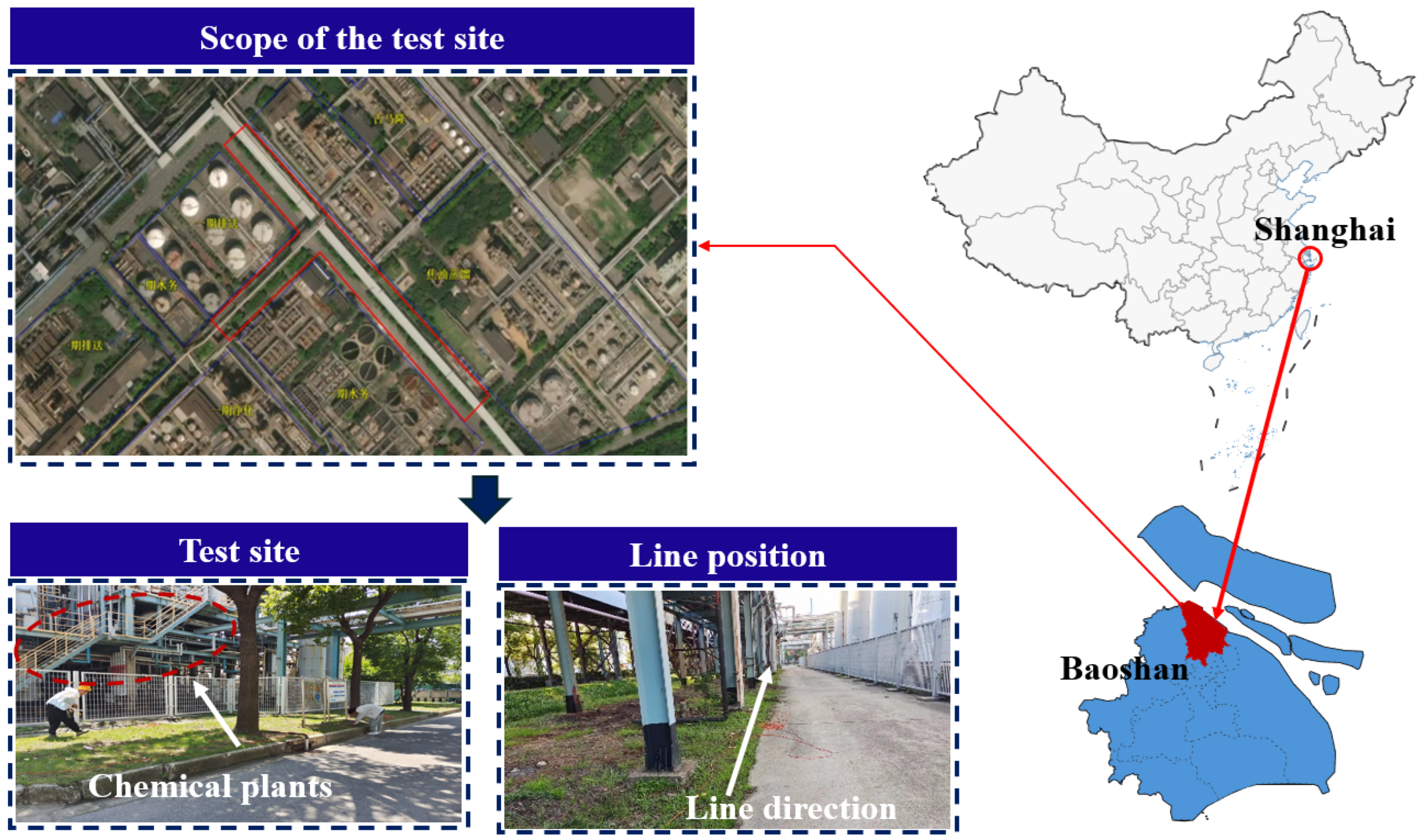
The study area is located at an industrial site in Baoshan District, Shanghai, situated within Quaternary alluvial clay deposits of the Yangtze River Delta. Geomorphologically classified as part of the dish-rim highland east of the ancient Songbei “Gangchen” paleo-coastal ridge, this open estuarine plain features gentle topography with minimal geological variation. The terrain slopes slightly northwest to southeast, maintaining an average surface soil thickness of approximately 300 m. As shown in Figure 1, the site is surrounded by functional zones including Phase I coal-refining facilities, water management infrastructure, and tar distillation operations. This investigation focuses on the red T-shaped roadway marked in Figure 1, comprising two main routes: a 200 m NW-SE axis and a 100 m NE-SW corridor.

Formerly housing chemical raw material production facilities, this site exhibits potential subsurface leakage of light non-aqueous phase liquids (LNAPLs) from undocumented underground infrastructure, posing significant environmental risks, including soil contamination and groundwater pollution. To address these challenges, this study implements ERT for long-term real-time monitoring of soil and groundwater resistivity variations. The system enables the following: early leakage detection through resistivity anomaly identification, visual tracking of remediation progress in contaminated zones, and predictive monitoring of potential pollutant migration pathways.

2.2. Working Principles of High-Density Electrical Resistivity Tomography

This investigation is based on electrical resistivity methods, with the primary principle for detecting organic contaminant leakage as follows: In oil-contaminated soil samples, the current conduction pathway can be considered as a composite system comprising soil particles, pore water, and oil. Since the resistivity of oil is significantly higher than that of water, an increase in oil saturation leads to greater occupation of pore spaces by oil, potentially blocking water-dominated conductive pathways, thereby elevating the bulk resistivity of contaminated soil [35]. Petroleum hydrocarbon contamination induces two key alterations: (1) a modification of the pore fluid composition and a restructuring of the double layer at soil–particle interfaces, and (2) resistivity variations caused by differences in the dielectric constant and electrical conductivity between petroleum products and pore water. Although soil resistivity is influenced by multiple factors—including water saturation, oil saturation, porosity, temperature, soil type, salinity, and organic content—the dominant controlling parameters follow this hierarchical order: water content, oil content, and porosity.

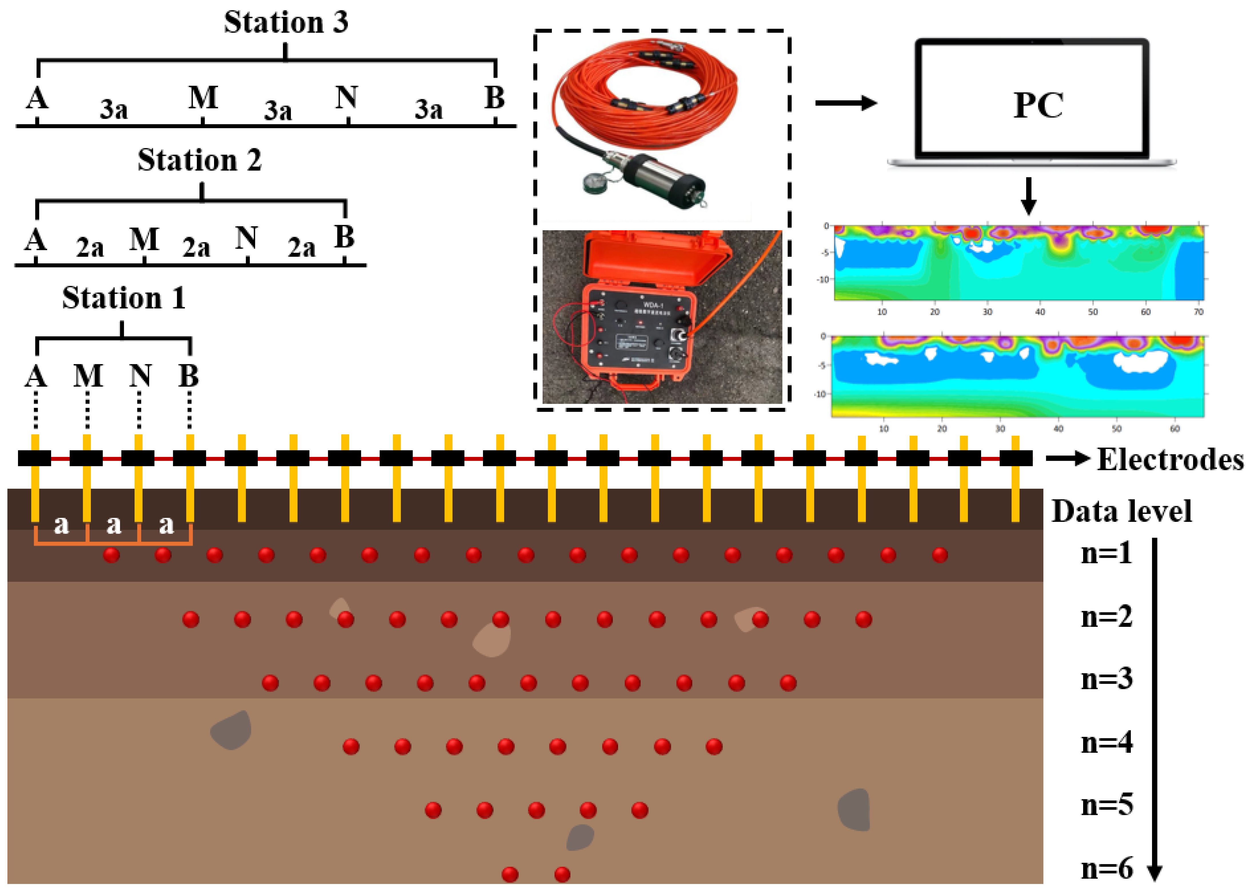
Electrical exploration methods can be divided into conductive electrical methods and inductive electrical methods. This investigation primarily adopts the high-density resistivity method (HDRM) from the conductive category. As a development of conventional electrical exploration techniques within the DC resistivity domain, HDRM fundamentally relies on electrical property differences in geological media to study the distribution patterns of subsurface conduction currents under applied electric fields [36], as shown in Figure 2. Compared to traditional electrical methods, HDRM is characterized by a high data volume. Through programmable electrode switchers controlled by microcomputers for automatic selection of current injection (A/B) and potential measurement (M/N) electrodes, this method achieves efficient data acquisition capable of rapidly collecting substantial raw data. It demonstrates high measurement accuracy, an extensive data collection capacity, rich geological information content, and superior production efficiency. A single-electrode deployment completes both vertical and horizontal 2D exploration processes, simultaneously reflecting lateral electrical property variations of subsurface media at specific depths and providing vertical electrical characteristic changes of stratigraphic lithology, thereby integrating the detection capabilities of both electrical profiling and electrical sounding methods.

Assuming a homogeneous subsurface medium with resistivity (ρ), when an electric current (I) is injected and a potential difference (ΔV) is measured, the apparent resistivity (ρ_a) is expressed as follows:

$${\rho }_{\mathrm{a}}=k{\displaystyle \frac{\Delta V}{I}}$$

(1)

where K represents the geometric factor determined by the electrode configuration [37]. Common electrode configurations in high-density resistivity surveys include the Wenner array, dipole–dipole array, and gradient array. The advantages and disadvantages of these configurations have been extensively analyzed in previous studies [38,39,40]. This study employs a four-electrode configuration, comprising current injection electrodes (A and B) and potential measurement electrodes (M and N), as illustrated in Figure 2.

In a homogeneous half-space medium, when current injection electrodes A and B transmit an electrical current into the subsurface, the potential difference (ΔV) measured between electrodes M and N allows for the calculation of the medium resistivity. The geometric factor (K), a constant determined solely by the electrode array geometry, can be expressed as follows:

$$k={\displaystyle \frac{2\pi }{\frac{1}{AM}-\frac{1}{AN}-\frac{1}{BM}+\frac{1}{BN}}}$$

(2)

where AM, AN, BM, and BN denote the distances between the respective electrodes.

2.3. ERT Configurations and Field Deployment

The “WGMD-9 High-Density Electrical Resistivity System” used in this study is a novel detection system developed by the Chongqing Benteng Numerical Control Technology Institute in China. This system utilizes the WDA-1 Super Digital DC Resistivity Meter as the control unit, which integrates with the WDZJ-4 multi-channel electrode switcher, distributed high-density cables, and electrodes to achieve distributed two-dimensional high-density resistivity measurements. The spacing, “a” (unit: meters), between current injection electrodes (A/B) and potential measurement electrodes (M/N) serves as a core parameter, determining the detection resolution and minimum depth. The number of profile layers, “n”, controls the vertical detection range through expanded electrode arrangements. During field measurements, electrodes are deployed at fixed intervals, “a”, along survey points and were connected to a programmable multi-electrode switcher via multi-core cables. Measurement signals from the electrode switcher are transmitted to the engineering resistivity meter, with results sequentially stored in random-access memory. The data are then transferred to a computer for post-processing, where the geometric factor (K) is calculated based on the electrode geometry corresponding to the layer number, “n” (see Equation (2)), ultimately completing the data processing workflow.

Based on the field conditions of the Baowu Carbon Industry site and the reconnaissance of the monitoring area, the high-density resistivity survey lines were systematically deployed. Monitoring wells MW4 and W5 are situated at the intersection of two main roads, leading to the arrangement of survey lines around the tar processing area, coal-refining area, and water management zone. A total of eleven survey lines were established: six in the tar processing area, including three transverse lines (each 60 m long with 2 m electrode spacing, labeled 1-1, 1-2, and 1-3), two densified lines (EL-1 and EL-2, measuring 60 m in length and with 2 m spacing), and one vertical line (20 m long with 1 m spacing, labeled a); three lines in the coal-refining area (each 60 m long with 2 m spacing, labeled 2-1, 2-2, and 3-1); and two lines in the water management zone (each 60 m long with 2 m spacing, labeled 2-3 and b).

2.4. Technical Workflow

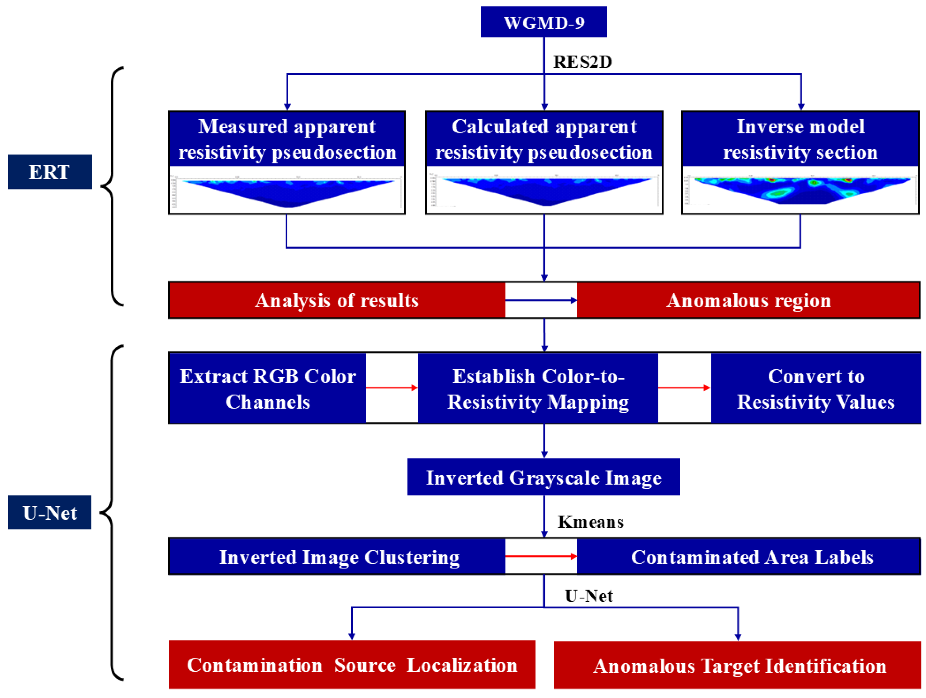
The technical workflow of this study is illustrated in Figure 3.

3. Field Test Analysis

3.1. ERT Data Interpretation Workflow

Field testing was conducted using the “WGMD-9 High-Density Resistivity System”, yielding extensive apparent resistivity datasets. During data acquisition, anomalies may arise from the following: (1) poor electrode contact with brick/gravel substrates in grassy areas, (2) power supply interference, or (3) high-resistivity surface obstructions (e.g., concrete/asphalt pavements). Such anomalous high-resistivity data were systematically eliminated to minimize interpretive bias. Post-electrode anomaly removal, datasets exhibiting voltage > 5000 mV or current > 1000 mA—attributable to overcurrent or electromagnetic interference—were further excluded. To mitigate random errors and verify data reliability, each survey line was measured twice, producing dual apparent resistivity (ρs) values per spatial measurement point. Data consistency was quantified using the sample standard deviation formula:

$$S=\sqrt{{\displaystyle \frac{1}{N-1}}{\displaystyle \sum _{i=1}^N{(X_i-\overline{X})}^2}}$$

(3)

The standard deviation (S) represents the dispersion of the two measurements (X₁) and (X₂), while $\overline{X}$ denotes their mean value. The percentage standard deviation (M), calculated as the ratio of S to $\overline{X}$, quantifies the relative deviation of the dual measurements from the mean apparent resistivity. Data points with M > 5% were discarded to ensure signal stability. The retained data were converted into inversion-compatible formats, requiring parameter specifications including the measurement method, electrode count, and electrode spacing during format conversion.

3.2. Analysis of Detection Results

The inversion process of high-density resistivity testing involves converting measured apparent resistivity data through format transformation, data preprocessing, forward modeling, and inversion calculations, ultimately generating apparent resistivity tomographic images. The formatted apparent resistivity data undergo preprocessing to eliminate outliers while retaining points with higher consistency. Using the optimal fitting method, an initial geoelectric section is defined to calculate theoretical apparent resistivity curves. These theoretical curves are then compared with measured curves, and parameters are iteratively adjusted to achieve optimal fitting results, producing the final inversion-derived resistivity tomographic images.

(1) Survey Line 2-1

Survey Line 2-1 spans 60 m in length and is aligned colinearly with monitoring wells. The subsurface in this area contains a substantial gravel layer beneath the soil stratum, with a surface soil moisture content higher than that of Line 1-1. This survey line traverses two concrete steps at its midpoint. An inversion analysis of the acquired data yielded the geoelectric cross-section presented in Figure 4.

The forward modeling results demonstrate a minimal discrepancy of 1.37% compared to the measured apparent resistivity values, indicating robust inversion performance. The subsurface exhibits distinct layered stratigraphy with resistivity values uniformly below 20 Ω·m, consistent with soil geotechnical reports and literature-derived resistivity values, showing no significant anomalies. As revealed by the inversion profile, localized high-resistivity zones occur at 22–26 m and 42–46 m along the survey line, corresponding to two reinforced concrete steps traversed by the measurement transect.

(2) Survey Line 2-2

Survey Line 2-2 extends 60 m in length, collinear with Survey Line 2-1 and the monitoring wells, traversing two concrete steps along its path. An inversion analysis of the acquired data yielded the geoelectric cross-section presented in Figure 5.

The forward modeling results show a 5.8% discrepancy compared to the measured apparent resistivity values, demonstrating good inversion performance. Distinct layered stratigraphy is observed beneath the surface. Due to the survey line crossing two reinforced concrete steps, localized high-resistivity zones are present at 18–22 m and 40–42 m along the line.

(3) Survey Line a

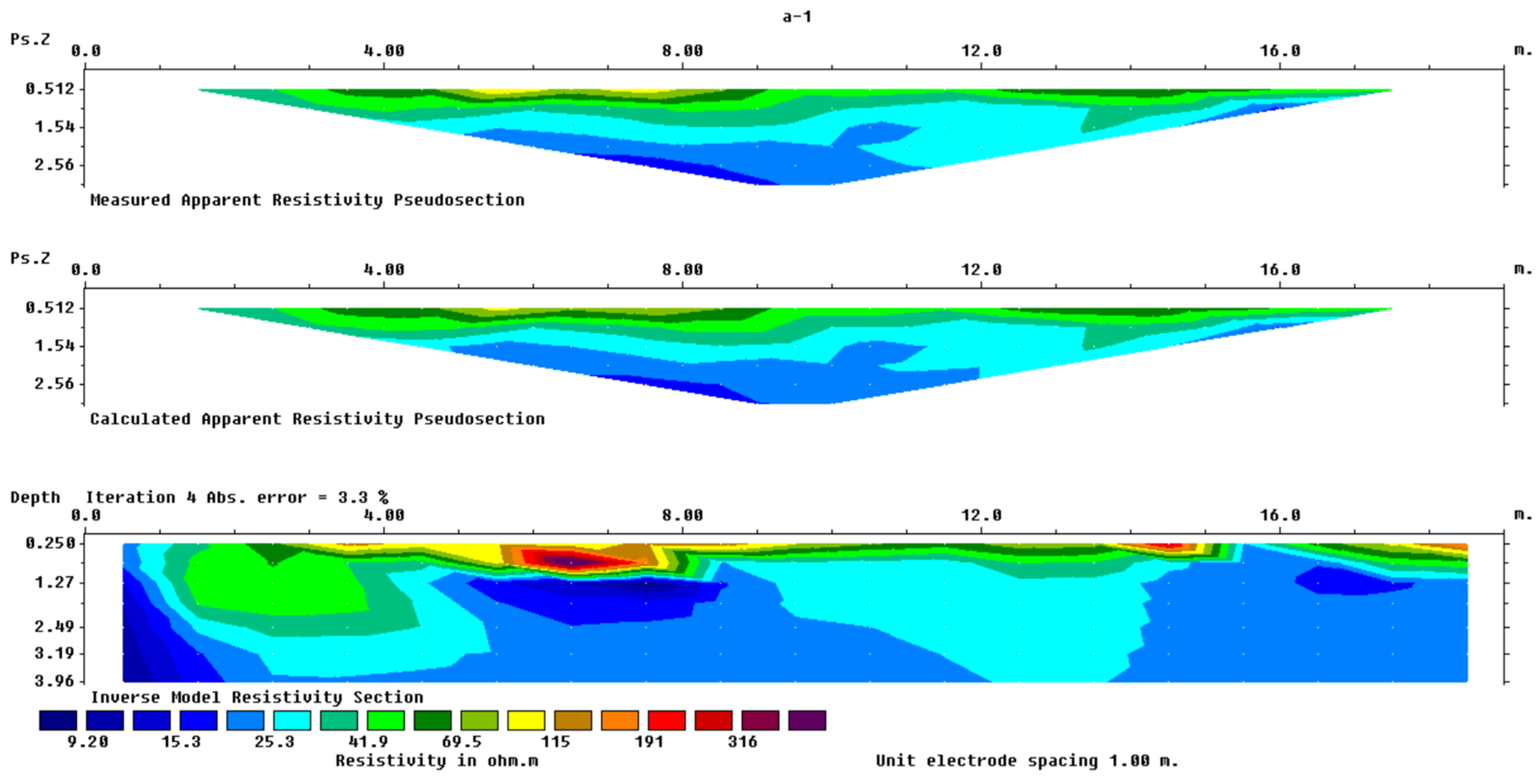
Survey Line a spans 20 m in length, positioned between Survey Lines 1-2 and 1-3. As it runs parallel to the water flow direction, this transverse line was designed to determine the horizontal distribution of subsurface contaminants. By collecting electrical resistivity data along the transverse direction, the horizontal extent and distribution characteristics of underground pollutants can be determined. The inversion analysis results of the acquired data are presented in Figure 6.

The forward modeling results demonstrate a minimal discrepancy of 3.3% compared to the measured apparent resistivity values, indicating satisfactory inversion performance. At a detection depth of 4 m, the imaging results do not exhibit strictly layered stratigraphy, with the majority of the subsurface composed of silty soil. This image reveals approximately circular high-resistivity zones at a burial depth of 1.5 m, necessitating verification of potential subsurface structures.

3.3. Re-Survey Testing in the Tar Processing Area

Based on the detection results of each survey line in Section 3.2, the key monitoring area (tar processing side) was re-examined after conducting a preliminary investigation of subsurface structures. Special attention was given to Survey Lines 1–3 and Densified Line 2. Repeating high-density resistivity surveys in this area helps monitor the evolution of subsurface contamination. By comparing resistivity data from different time periods, the migration and diffusion of subsurface pollutants can be identified. This provides critical insights into the activity level of pollution sources, the extent of contaminant spread, and groundwater flow directions—particularly important for pollution monitoring at industrial sites involving groundwater protection, where re-survey lines can track contamination trends and detect potential risks of spreading.

A time-lapse resistivity analysis offers more detailed information on subsurface contamination. By conducting a temporal analysis of resistivity data from different periods, the transport and variation of pollutants in the subsurface medium are revealed. This helps determine the migration velocity, diffusion range, and pathways of contaminants, thereby providing a scientific basis for developing effective remediation strategies.

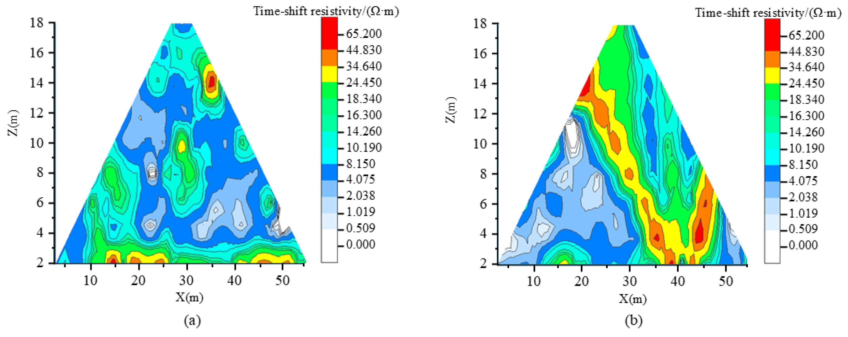
After completing the survey, all 60 electrode points were marked with small red flags. Two rounds of testing were conducted one week apart. The absolute difference in apparent resistivity was calculated. The results are presented as numerical differences in resistivity changes between the two tests: positive values indicate an increase in resistivity, while negative values indicate a decrease. According to Figure 7a, the absolute resistivity change plot for Survey Line 1-3 shows a reduction of 10–40 Ω·m in near-surface resistivity, likely due to increased soil moisture from rainfall during the testing period. Figure 7b reveals localized resistivity increases of 5–10 Ω·m at depths of 2–14 m along Densified Line 2, possibly caused by changes in contaminant infiltration.

Relative resistivity is calculated as follows: (difference in absolute resistivity) ×/(first apparent resistivity value + second apparent resistivity value). As shown in Figure 8, the variation patterns of the two survey lines can directly reveal locations with significant resistivity change rates. For operating industrial plants, a time-lapse resistivity analysis can also assist in evaluating environmental risks and formulating relevant emergency plans. By real-time monitoring of subsurface medium changes, it can better predict the diffusion trends of contaminants, enabling timely implementation of corresponding countermeasures to safeguard surrounding residents and ecological environment safety.

4. Construction of Deep Learning Database

Upon completing field testing operations, the core focus of laboratory work involves achieving an automated, efficient, and precise identification of contaminated soil regions based on resistivity images. Given that the research subject consists of resistivity images from contaminated sites, computer vision technology was selected as the primary solution for data interpretation. The three fundamental tasks of computer vision are classification, detection, and segmentation. Classification determines the presence of contaminated areas within images, addressing problems at the image level. Object detection locates contaminated regions within images, presenting results through confidence scores and rectangular bounding boxes to solve spatial positioning challenges. Segmentation constitutes pixel-level classification, resolving issues at the pixel scale by providing detailed shapes and contours of contaminated areas, which enables a visual assessment of the soil contamination status and facilitates further quantitative analysis of contamination characteristics. Through systematic analysis and verification, this study has transformed the contaminated area identification challenge into an image segmentation problem. A high-performance semantic segmentation model was trained and subsequently applied to perform inference on resistivity inversion images, automatically delineating contaminated zones to support contamination assessments and decision-making processes.

The emergence of large-scale open datasets and advancements in high-performance GPU technology have established convolutional neural networks (CNNs) as the predominant architecture in computer vision over the past decade. When integrated with fully supervised learning paradigms, CNNs have become the preferred approach for automated image interpretation tasks in civil engineering applications [41,42,43,44,45]. The critical requirement for CNN-based supervised training lies in constructing high-quality databases. This section details the development process of a specialized database containing original resistivity inversion images and label maps generated through clustering algorithm assistance.

4.1. ERT Data Preprocessing

Prior to inversion, the raw ERT measurements undergo a series of preprocessing steps to reduce noise and correct artifacts: (1) Data filtering and outlier removal: Extremely high or negative apparent resistivity values, often resulting from poor electrode contact or instrumental errors, are identified and removed using a threshold-based approach and manual quality inspection; (2) Stacking and signal averaging: Multiple measurements are stacked to improve the signal-to-noise ratio (SNR), particularly in regions with high contact resistance; (3) Geometric and topographic corrections: Electrode positions are adjusted based on differential GPS data and corrected for terrain effects using a topographic correction module in the inversion software; and (4) Reciprocity checks: Forward and reverse measurements are compared to identify inconsistent data, which are then excluded from inversion. These preprocessing techniques significantly enhance data reliability and ensure stable convergence during the subsequent inversion and imaging stages.

4.2. Contamination Zone Analysis

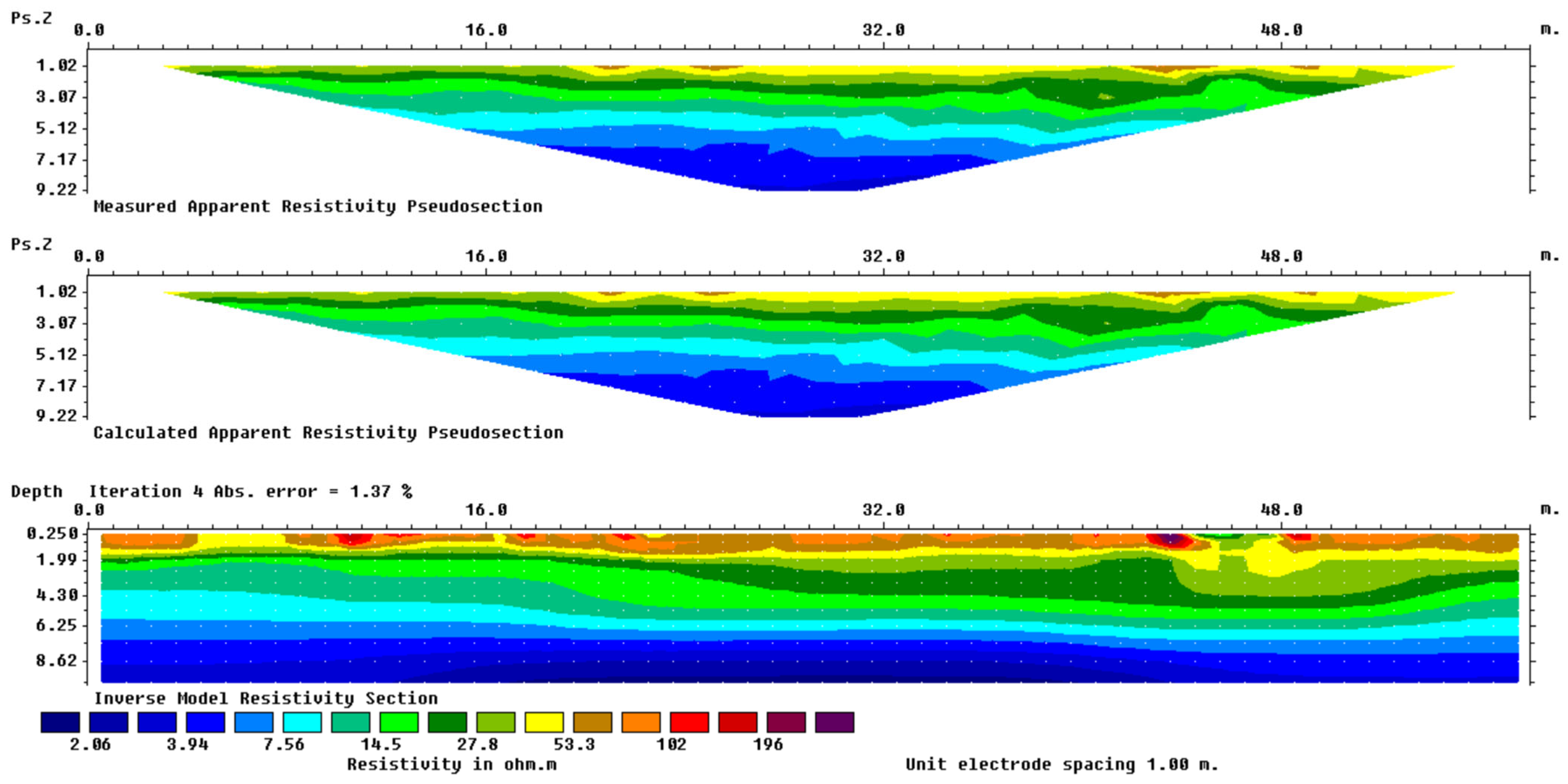
Figure 9 presents the measured apparent resistivity cross-section and calculated apparent resistivity cross-section obtained from high-density resistivity testing at a specific survey point. Figure 9a displays the original apparent resistivity contour map with resistivity values ranging from 5 to 25 Ω·m, exhibiting significant lateral heterogeneity. A distinct low-resistivity zone (<10 Ω·m) is observed in the central portion of the profile (horizontal position: 10–15 m; depth: 0–5 m), potentially caused by loose sediments or aquifers. In contrast, high-resistivity zones (>20 Ω·m), identified at both sides (positions: 0–5 m and 20–25 m), may correspond to dry compacted soil layers or bedrock outcrops. Figure 9b shows the computed apparent resistivity distribution, where data processing enhances the spatial characteristics of the low-resistivity anomaly (depth: 3–7 m). Compared with Figure 9a, these results minimize topographic and measurement configuration artifacts, more accurately reflecting the true electrical property variations of subsurface media.

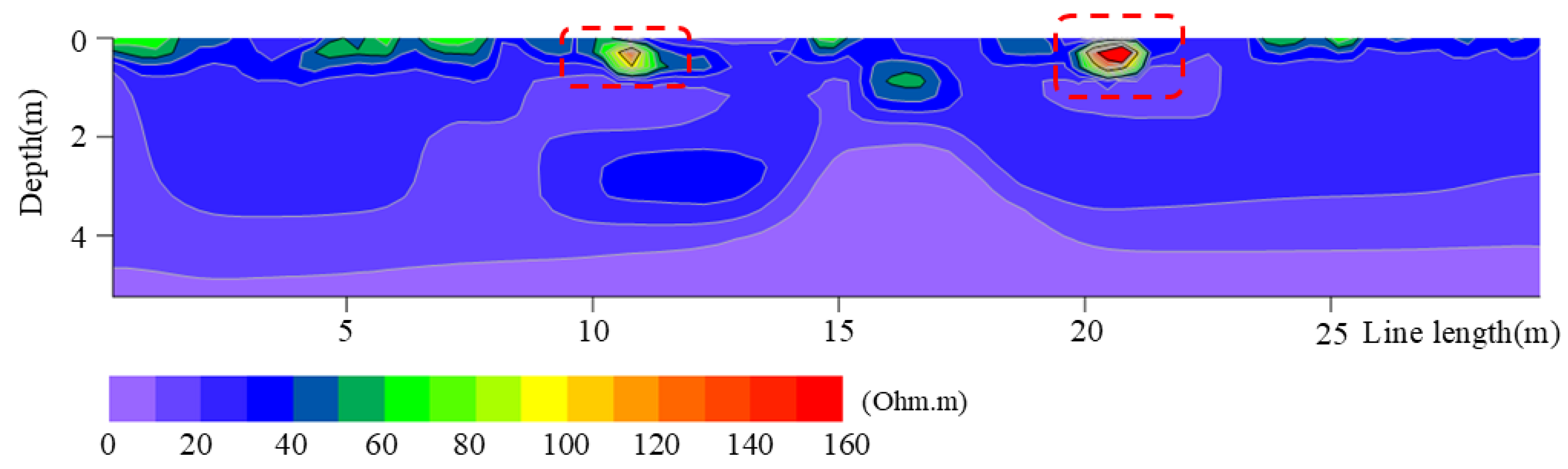
The inversion of the apparent resistivity test results from Figure 9 using the Surfer software 15 yielded the inversion-imaged chromatogram shown in Figure 10. After four iterations with an absolute error of 2.3%, the results clearly characterize the subsurface electrical structure of the study area. The results show a medium-resistivity (15–20 Ω·m) surface overburden layer at 0–1.5 m in depth. A distinct low-resistivity anomaly zone (5–10 Ω·m) is developed at 1.5–3.5 m in depth, which is most prominent at horizontal positions at 10–15 m along the survey line. Below 3.5 m in depth, the resistivity gradually increases to above 25 Ω·m, reflecting the undulating characteristics of the bedrock surface. Particularly noteworthy are two pronounced high-resistivity anomalies (>35 Ω·m) developed within the depth range of 1.5–4 m at horizontal positions 5–8 m and 18–22 m, with resistivity values significantly higher (approximately 2–3 times) than the surrounding media. The inversion results demonstrate excellent consistency with the apparent resistivity profile in Figure 10 while providing higher-resolution electrical structure details, offering reliable evidence for identifying potential water-bearing structures and delineating bedrock weathering interfaces.

4.3. Inversion Image Clustering Based on K-Means Algorithm and Binary Contamination Area Label Map Generation

First, the color intensity or values of the inversion image in Figure 10 were mapped to a single grayscale level to generate a single-channel grayscale image, as shown in Figure 11. In the grayscale image, the intensity of each pixel is represented by a single value ranging from 0 (black) to 255 (white) for an 8-bit grayscale image, reflecting the brightness of that pixel.

The grayscale inversion image is subsequently input into the K-means algorithm [46] to achieve clustering of different soil regions. The algorithm primarily consists of three steps:

(1) K-value selection: Determine the number of clusters (K) for classification.

(2) Centroid initialization: Randomly select K data points (pixels) as initial centroids.

(3) Iterative optimization: First assign each data point (pixel) to its nearest centroid. Then, calculate new centroids for each cluster. Repeat these steps until the centroid positions no longer change significantly or the preset maximum number of iterations is reached. Finally, examine the clustering results, and manually adjust the K-value to obtain optimal clustering outcomes. The clustering results for the example image in Figure 11 are shown in Figure 12. It can be clearly observed that multiple connected regions have formed in the resistivity inversion image, which contain potential target contamination zones.

Based on the aforementioned clustering results, the clusters of interest are extracted as contaminated areas to obtain a binary label map. The key steps involve creating a blank image with the same dimensions as the original data or inversion image and iterating through each pixel in the image—if the pixel (or data point) belongs to the target cluster, it is set to 1; otherwise, it is set to 0. This process yields a binary image of the contamination area labels, as shown in Figure 13, where the white areas (value 255) represent contaminated zones, and the black areas (value 0) denote non-contaminated zones.

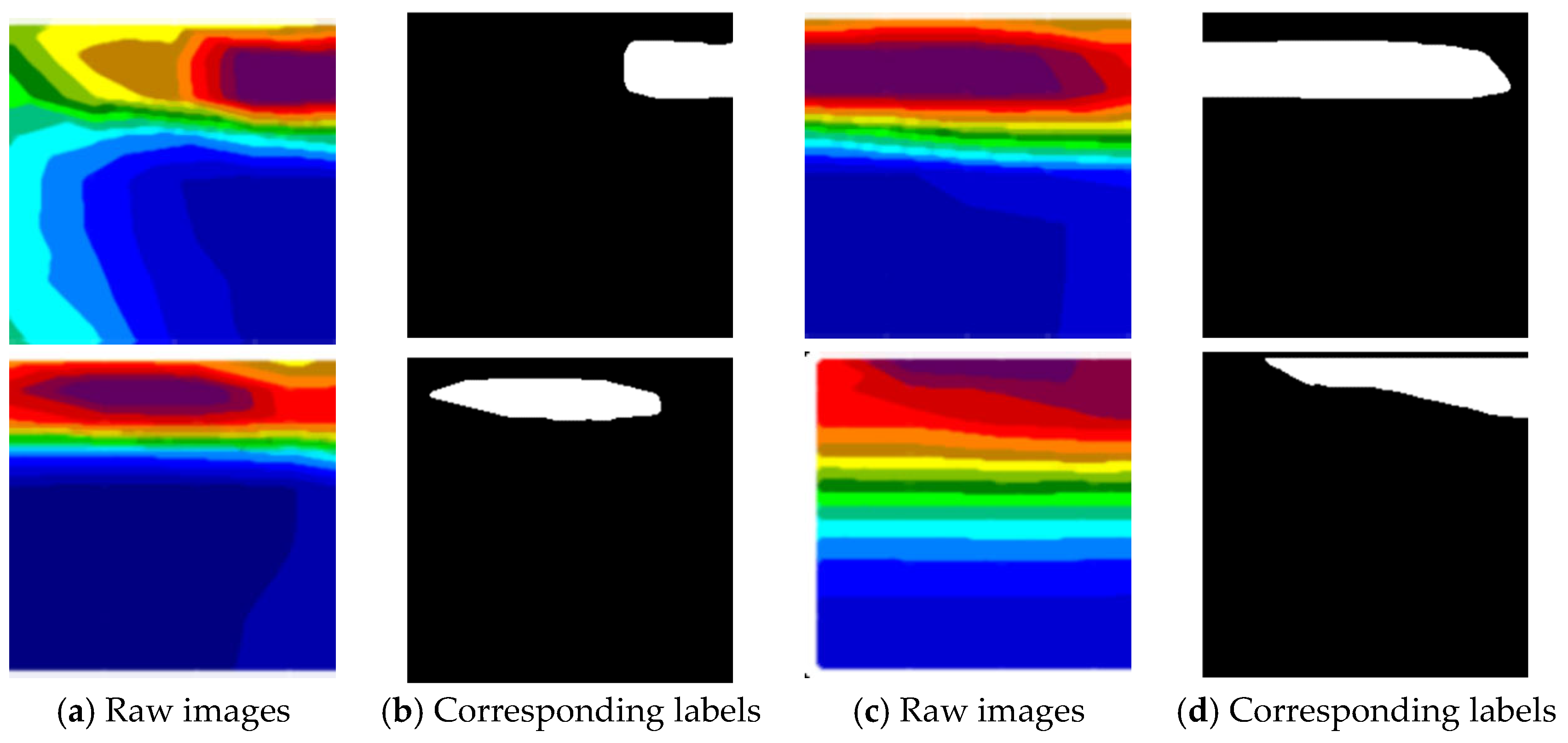
Following the aforementioned procedures, each original inversion image is processed to generate corresponding labels. Considering that ultra-high-resolution images impose extreme hardware requirements for CNN learning and inference while significantly reducing model training and testing speeds, the image-label pairs, composed of Figure 10 and Figure 13, are partitioned using a sliding window approach. This process yields 204 pairs of 512 × 512 original inversion images with their corresponding labels, ultimately forming the final deep learning database. Four representative samples are displayed in Figure 14. It should be noted that the original inversion images in the database were stored in 24-bit PNG format, while the label images maintain the previously described 8-bit PNG format.

The dataset was further partitioned into training and testing sets for CNN application, following an 8:2 ratio. This division yielded 163 training samples and 41 testing samples. Throughout the training process, the testing samples remained completely isolated to ensure a comprehensive and unbiased evaluation of the model’s contamination identification performance. It is important to note that the UNet model does not explicitly classify NAPL types. Instead, it identifies regions with anomalous resistivity values, which may result from either single-type or mixed-type NAPL contamination.

5. Establishment, Training, and Testing of Deep Learning Model

UNet [34], proposed by Ronneberger et al., is a deep learning model widely applied in image segmentation tasks. Its core architecture consists of symmetrical encoder and decoder components, with the network structure illustrated in Figure 15a. Figure 15b details the structural components of UNet, where Conv represents the convolution operation, max pooling denotes the max pooling operation, BN stands for batch normalization, and ReLU and Sigmoid are activation functions. The encoder (primarily composed of Blocks 2–5) progressively extracts high-level semantic features through successive convolution and downsampling operations (max pooling), while reducing the spatial resolution to decrease the computational load. Blocks 2–5 are essentially convolutional blocks, each containing two or three convolutional layers. The convolution operation, characterized by weight sharing and translation invariance, can effectively extract local features of contamination data regardless of the spatial distribution of pollutants. The max pooling operation within the convolutional blocks reduces feature map dimensions, gradually expanding the model’s receptive field and generating a series of soil contamination feature maps at different scales. This expansion of the network’s receptive field enhances its understanding of long-range dependencies in contamination data. The decoder (mainly comprising Blocks 7–10) gradually restores the image resolution through upsampling operations and achieves a refined fusion of multi-scale features by incorporating skip connections (red dashed arrows) that integrate features from different stages of the encoder. Blocks 7–10 progressively restore feature maps to their original dimensions through interpolation operations, followed by channel-wise concatenation with multi-scale feature maps extracted from the encoder and subsequent convolution operations.

The entire network adopts a lightweight design, with an encoder identical to VGG [47] (specifically, VGG-16, as shown in Figure 15), featuring a relatively small parameter scale that maintains high computational efficiency and inference speed. Meanwhile, UNet ensures high segmentation accuracy by directly concatenating and fusing the encoder’s low-level high-resolution features with the decoder’s high-level low-resolution features through skip connections. Another important reason for selecting UNet in this study is its exceptional performance in small-sample learning scenarios, which stems from two key advantages: First, the skip connections and symmetrical architecture enable full utilization of multi-scale information from limited annotated data, reducing reliance on large-scale training samples through feature reuse—particularly suitable for the contaminated soil resistivity image data in this study. Second, UNet directly optimizes pixel-level predictions through end-to-end training, and when combined with data augmentation strategies, can further enhance the model’s robustness to sample scarcity.

5.1. Algorithm Performance Evaluation Metrics

In the semantic segmentation task of contaminated site images, Acc serves as the most intuitive evaluation metric, reflecting the overall correctness of pixel-level category predictions by the model. It is defined as the ratio of correctly predicted pixels to the total number of pixels in the test images, with the mathematical expression given in Equation (4). Pre measures the proportion of correctly predicted positive-class pixels among all pixels predicted as positive, as defined in Equation (5). Rec quantifies the proportion of actual positive-class pixels that are correctly identified by the model, specified in Equation (6). The f1 represents the harmonic mean of precision and recall, providing a comprehensive evaluation of model performance across both metrics, given in Equation (7). The mIoU, a widely adopted evaluation metric in image semantic segmentation tasks, measures the spatial overlap between predicted segmentation results and ground truth annotations, defined in Equation (8).

$$Acc={\displaystyle \frac{TP+TN}{TP+FP+TN+FN}}$$

(4)

$$Pre={\displaystyle \frac{TP}{TP+FP}}$$

(5)

$$Rec={\displaystyle \frac{TP}{TP+FN}}$$

(6)

$$f1=2\times {\displaystyle \frac{Pre\times Rec}{Pre+Rec}}$$

(7)

$$mIoU={\displaystyle \frac{1}{C}}{\displaystyle \sum _{c=1}^C\frac{T{P}_c}{T{P}_c+F{P}_c+F{N}_c}}$$

(8)

where TP (true positive) represents the number of correctly predicted positive-class pixels, TN (true negative) denotes the number of correctly predicted negative-class pixels, while FP (false positive) and FN (false negative) correspond to misclassified positive-class and negative-class pixels, respectively. C denotes the category, specifically, foreground or background pixels. Here, C takes the value 2, indicating that this study treats the segmentation of contaminated and non-contaminated areas as a binary segmentation problem.

5.2. Model Training and Hyperparameter Optimization

The experiments in this study were conducted on a professional workstation running the Windows 10 operating system, equipped with a 12th Gen Intel(R) Core(TM) i9-12900KF CPU (Intel, Santa Clara, CA, USA) and two NVIDIA RTX 3090 GPUs (Nvidia, Santa Clara, CA, USA). All algorithms were implemented in Python 3.9, with the K-means clustering algorithm based on the scikit-learn library and the UNet algorithm built upon the PyTorch 2.4.0 framework.

The UNet hyperparameters were configured as follows: epochs set to 50; batch size set to 8; initial learning rate of 0.0001, which decayed to 0.00001 after 30 training epochs; the loss function employed Dice Loss to adequately account for class imbalance (where contaminated areas represent a relatively small portion of the entire site); and during training, image–label pairs were randomly horizontally or vertically flipped with a 50% probability to enhance model robustness and ensure optimal training outcomes. The training process is illustrated in Figure 16. The loss function decreased sharply during the first 5 epochs, exhibited fluctuating declines between epochs 6–25, and gradually converged thereafter. Conversely, the IoU metric showed rapid initial improvement in the early epochs, followed by fluctuating increases until stabilization. These training dynamics demonstrate that the UNet model successfully converged on our custom dataset.

Based on testing conducted with the trained UNet model, the evaluation results are as follows: mIoU reached 86.58%, Acc achieved 99.42%, Pre attained 75.72%, Rec reached 76.80%, and f1 registered 76.23%. Additionally, this study evaluated the inference speed of UNet on contaminated soil resistivity images, obtaining a processing rate of 15.51 images per second. These results demonstrate UNet’s exceptional suitability for automated segmentation tasks in contaminated site identification, exhibiting outstanding accuracy and efficiency.

Qualitative testing results of the model are shown in Figure 17. The segmentation outputs from UNet show high consistency with the actual contaminated areas, further validating the model’s superior contamination identification performance.

To further validate the optimal selection of two core hyperparameters in the UNet training process, learning rate, and batch size, a series of hyperparameter optimization experiments were conducted, with results documented in

Table 1. Hyperparameter optimization experimental results.

Hyperparameter Configurations	mIoU (%)	Acc (%)	Pre (%)	Rec (%)	f1 (%)
initial learning rate = 0.0001 batch size = 8	86.58	99.42	75.72	76.80	76.23
initial learning rate = 0.001 batch size = 8	82.94	98.57	73.09	75.48	73.66
initial learning rate = 0.01 batch size = 8	79.30	97.23	67.82	74.38	69.74
initial learning rate = 0.0001 batch size = 4	86.34	99.37	75.47	76.63	76.01
initial learning rate = 0.0001 batch size = 2	83.48	98.60	73.06	76.91	74.88

. The initial learning rate was tested at three values, 0.0001, 0.001, and 0.01, while the batch size, determined by the workstation configuration, was evaluated at 8, 4, and 2. It should be noted that after 30 training epochs, the learning rate was adjusted to 1/10 of its initial value for each configuration. When employing a smaller initial learning rate (0.0001) with a batch size of 8, the model achieved optimal performance (mIoU 86.58%). As the learning rate increased to 0.001 and 0.01, mIoU decreased by 3.64% and 7.28%, respectively, while f1 declined by 2.57% and 6.49%, indicating that excessively large learning rates destabilize the optimization process. Notably, with a fixed learning rate of 0.0001, reducing the batch size from 8 to 4 had a limited impact on accuracy (0.24% mIoU reduction), but further reduction to 2 caused significant performance degradation (3.10% mIoU decrease). This demonstrates that moderate batch sizes help maintain gradient update stability. Experimental results confirm that for contaminated site segmentation tasks, the UNet model exhibits considerable sensitivity to hyperparameter configuration. The best practice is to use a small learning rate (0.0001) with a large batch size (8).

Further investigation examined the impact of the model’s encoder on segmentation performance. While the UNet architecture, shown in Figure 15, employs VGG-16 as its encoder, we additionally considered VGG-13 and VGG-19 configurations. Training and testing maintained identical optimal hyperparameters established previously. With VGG-13 as the encoder, UNet achieved an mIoU of 85.86%, an Acc of 99.26%, a Pre of 75.22%, an Rec of 76.26%, and an f1 of 75.68%. Using VGG-19 yielded an mIoU of 85.79%, an Acc of 99.22%, a Pre of 75.45%, an Rec of 76.03%, and an f1 of 75.70% [P6.1]. These results demonstrate reduced segmentation accuracy for contaminated areas with both VGG-13 and VGG-19 encoders. Therefore, the optimal configuration employs VGG-16 as UNet’s backbone architecture.

5.3. Model Inference and Case Validation

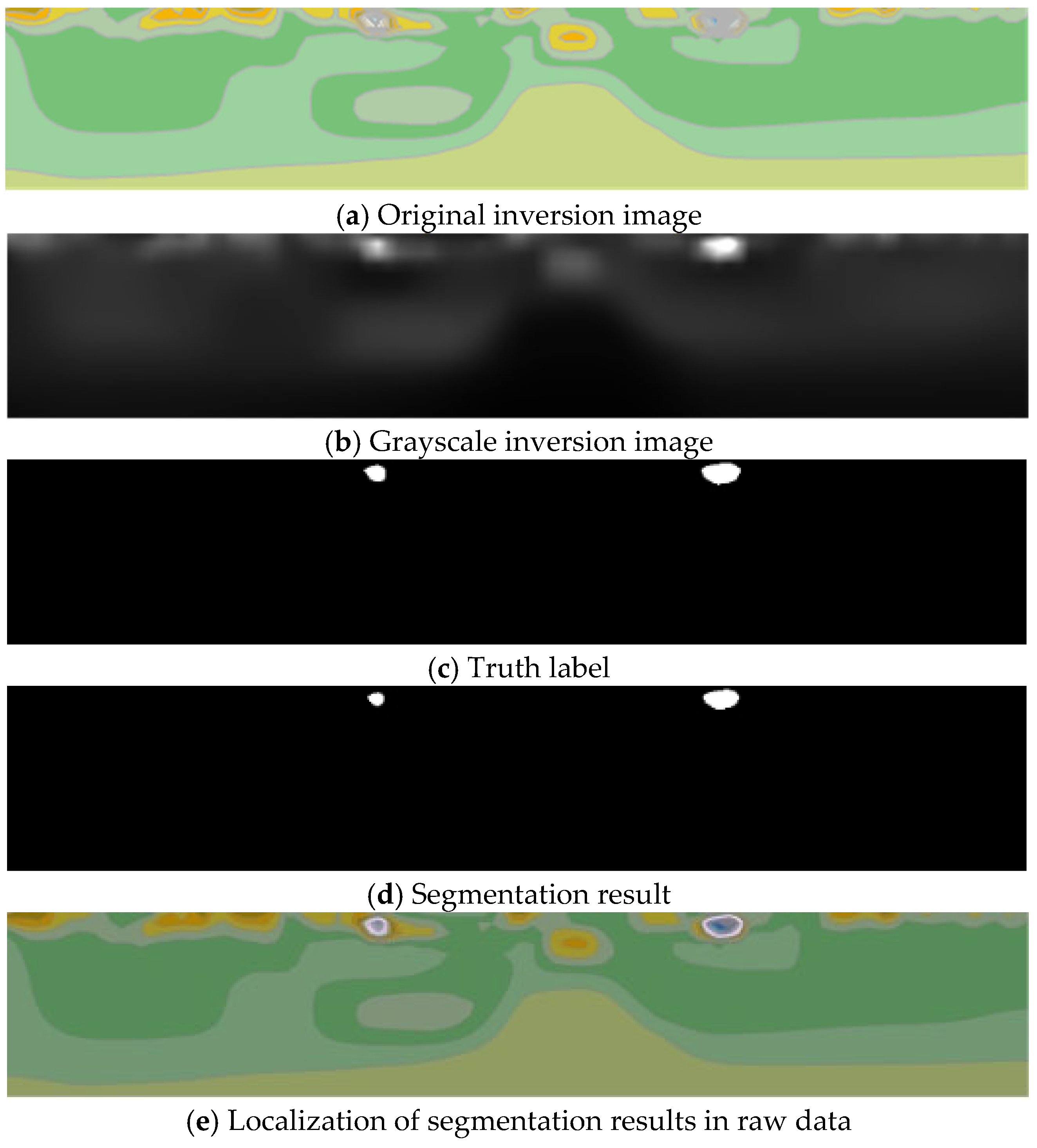
To verify the applicability and reliability of UNet in practical contaminant detection tasks, this section presents a comprehensive case study. Figure 18 displays the original image based on high-density electrical method inversion, the ground truth annotation, and the segmentation results from the deep learning model for a specific site. The target anomalies to be identified are the two white regions in Figure 18c. After feeding the original image into the UNet recognition network, the output is shown in Figure 18d. By overlaying the identification results with the original image (where pink represents the localized contaminant plumes and blue denotes the target contaminants to be localized), it is evident that the network achieves robust segmentation and localization performance.

Traditional NAPL identification approaches, which provide high specificity but are time-consuming, invasive, and costly, primarily rely on direct sampling. Geophysical methods such as ERT have also been applied by interpreting resistivity anomalies manually; however, this process is often subjective and labor-intensive, especially for large datasets. Geostatistical methods, like kriging or Bayesian approaches, require prior assumptions about spatial continuity and distribution, which may not hold in complex contaminated sites. In contrast, the proposed UNet-based model enables rapid and automated identification of resistivity anomaly zones associated with potential NAPL contamination. This significantly improves efficiency and reproducibility, particularly in field-scale surveys. Future work will focus on integrating additional site knowledge and multi-physics data to enhance classification performance.

5.4. Comparison with Mainstream Models

To validate the strong applicability and high accuracies of the UNet adopted in this study for pollution detection tasks, a series of comparative experiments were conducted. Four representative semantic segmentation models, LinkNet [48], PSPNet [49], DeepLabV3 [50], and DeepLabV3+ [51], were selected for comparison. To ensure fairness, all models were trained and tested on the same workstation using identical datasets. For clarity of discussion, we focus on two core accuracy metrics: mIoU and f1. The experimental results are recorded in the table below.

As shown in

Table 2. Comparison of four representative semantic segmentation models.

Models	mIoU (%)	f1 (%)
UNet	86.58	76.23
DeepLabV3	84.77	73.53
DeepLabV3+	84.85	73.91
PSPNet	84.38	74.70
LinkNet	85.66	75.71

, UNet demonstrates clear superiority across both evaluation metrics compared to all other models. It outperforms DeepLabV3 by significant margins of 1.81% in mIoU and 2.70% in f1, while also maintaining advantages of 1.73% in mIoU and 2.32% in f1 against DeepLabV3+. When compared to PSPNet, UNet shows even stronger dominance in segmentation accuracy, with a 2.20% higher mIoU, along with a 1.53% f1 improvement. Even against the closest competitor LinkNet, UNet preserves a consistent lead of 0.92% in mIoU and 0.52% in f1, solidifying its position as the top-performing model with the highest absolute scores in both critical segmentation metrics.

6. Conclusions

Focusing on the requirements for precise identification and dynamic monitoring of non-aqueous phase liquid (NAPL) contamination in low-permeability clay sites, this study systematically addresses the limitations of traditional detection methods in complex geological environments through methodological innovation, technical integration, and engineering validation. The findings offer innovative solutions for precise identification and remediation of contamination in complex geological settings. The core findings are summarized as follows:

(1) A unified technical system integrating high-density ERT and an improved UNet deep learning model was developed, forming a complete workflow from data acquisition to intelligent interpretation. This effectively resolves the challenges of weak electrical anomalies and high noise in clay-rich environments, enabling an accurate reconstruction of contamination plume morphology.

(2) The improved UNet model, incorporating multi-scale feature fusion and skip connections, attained an mIoU of 86.58%, an Acc of 99.42%, a Pre of 75.72%, an Rec of 76.80%, and an f1 of 76.23% in contamination zone segmentation. Compared to manual interpretation in traditional geophysical exploration, this approach enhances efficiency by over 80% while significantly reducing misjudgment rates.

(3) Time-lapse resistivity imaging and case validation at a contaminated site demonstrate the method’s capability to dynamically track contaminant migration with positioning errors below 0.5 m. This provides spatial decision-making support for remediation, reducing costs by 60% compared to conventional borehole sampling and driving the transition toward non-destructive, intelligent environmental detection.