
Experimental Investigation in Drag Coefficient of Cubes


 ,
,
Abstract
1. Introduction
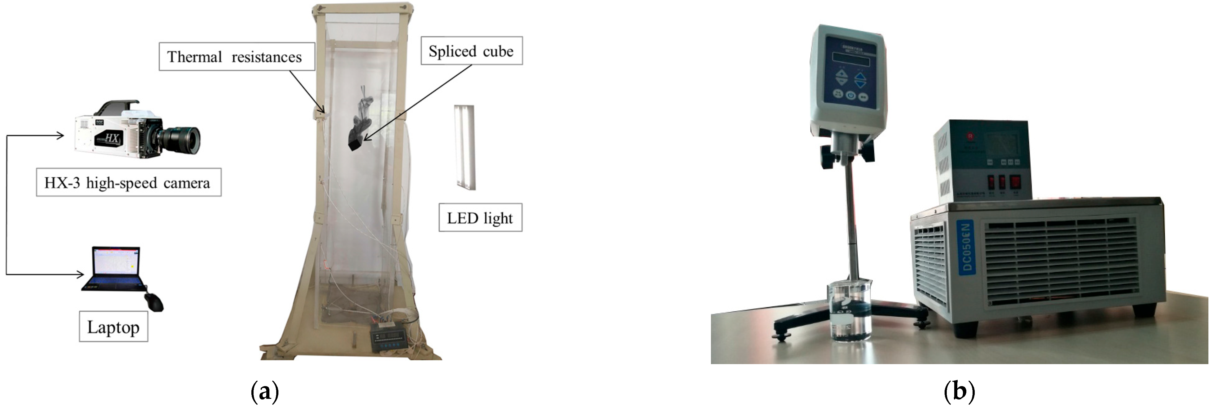
2. Experimental Facility and Procedure
3. Calibration of Experimental Facility
4. Results and Discussion
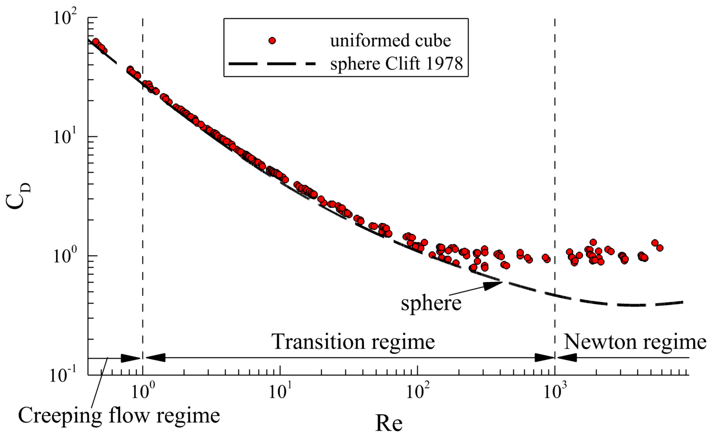
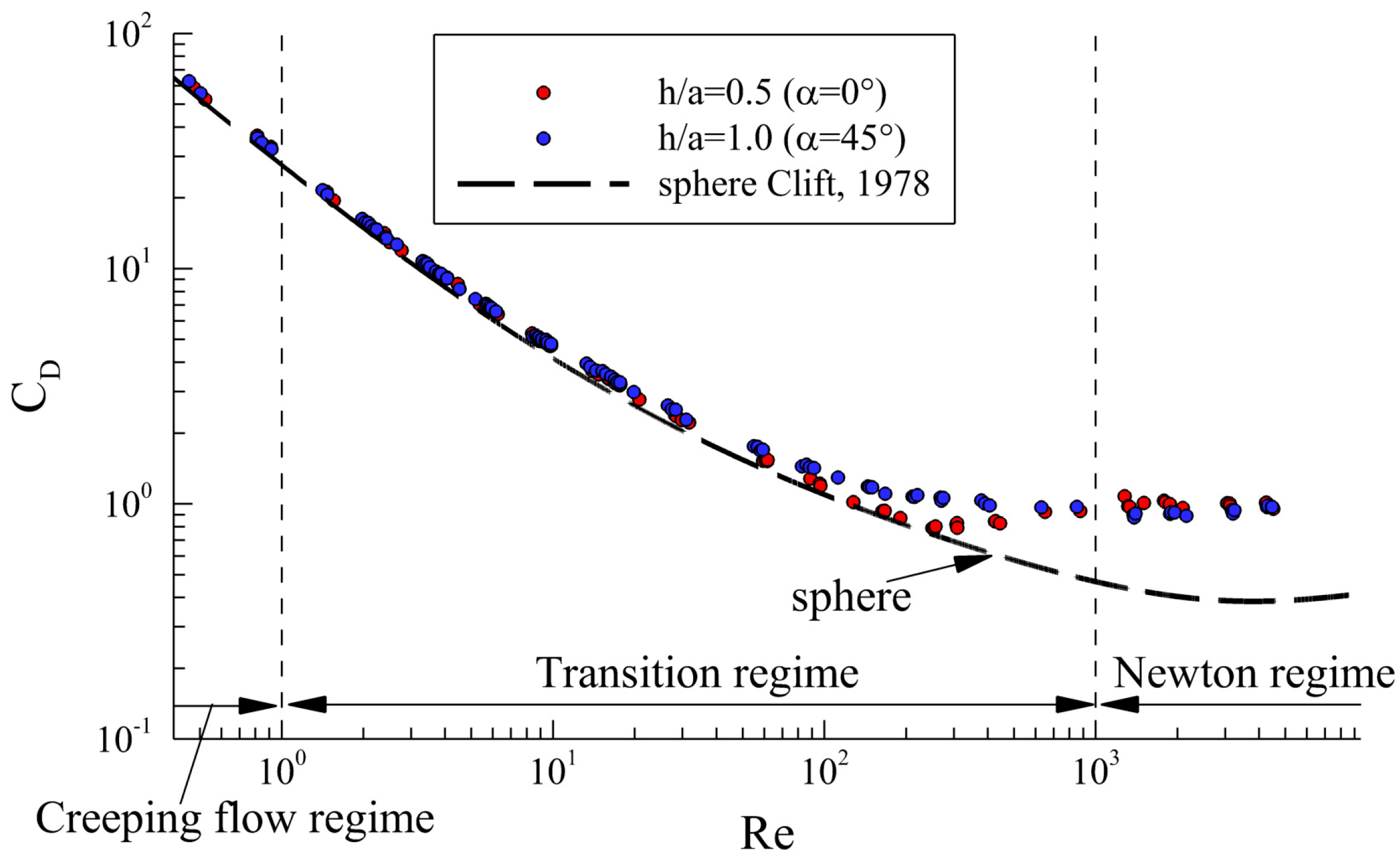
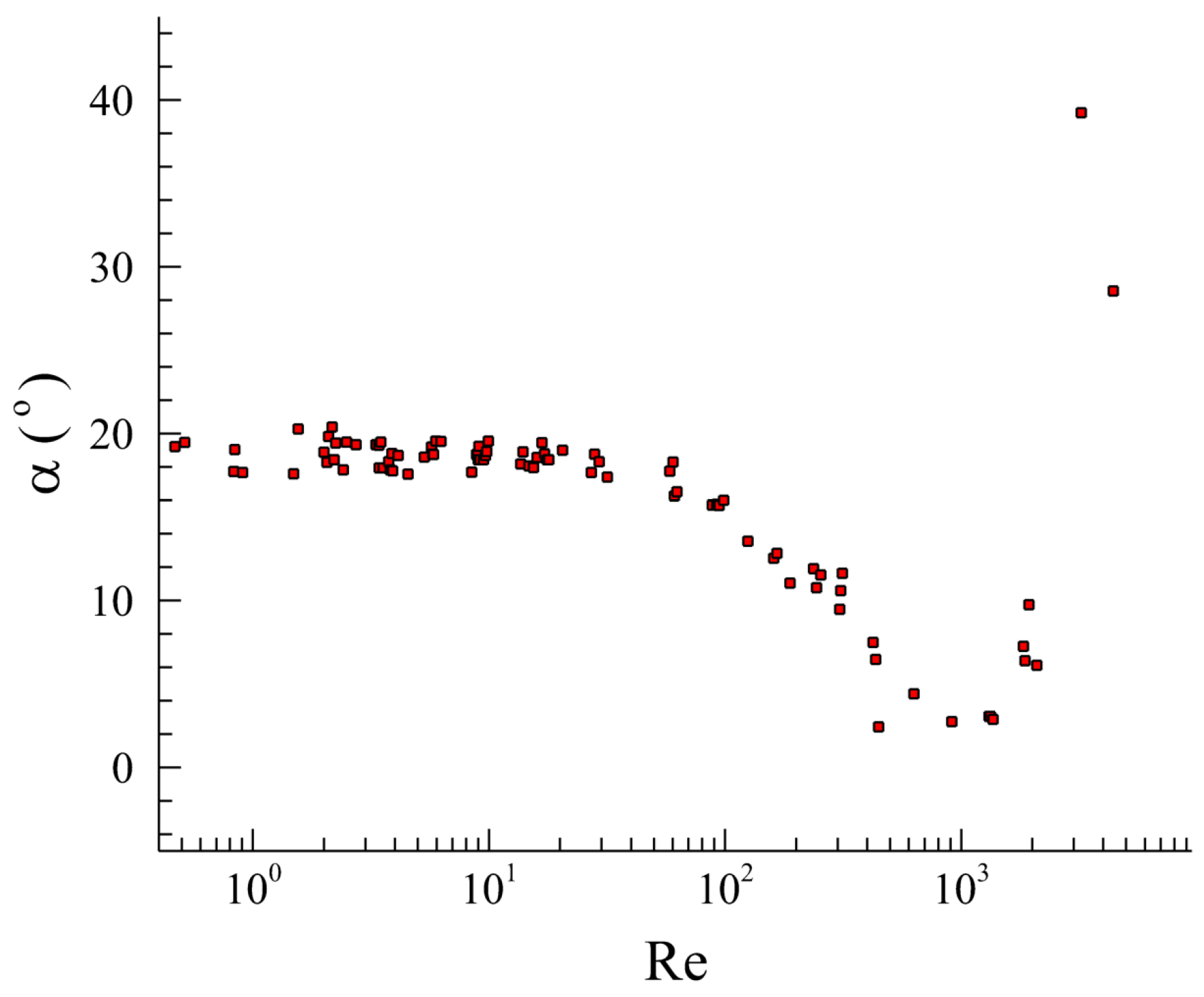
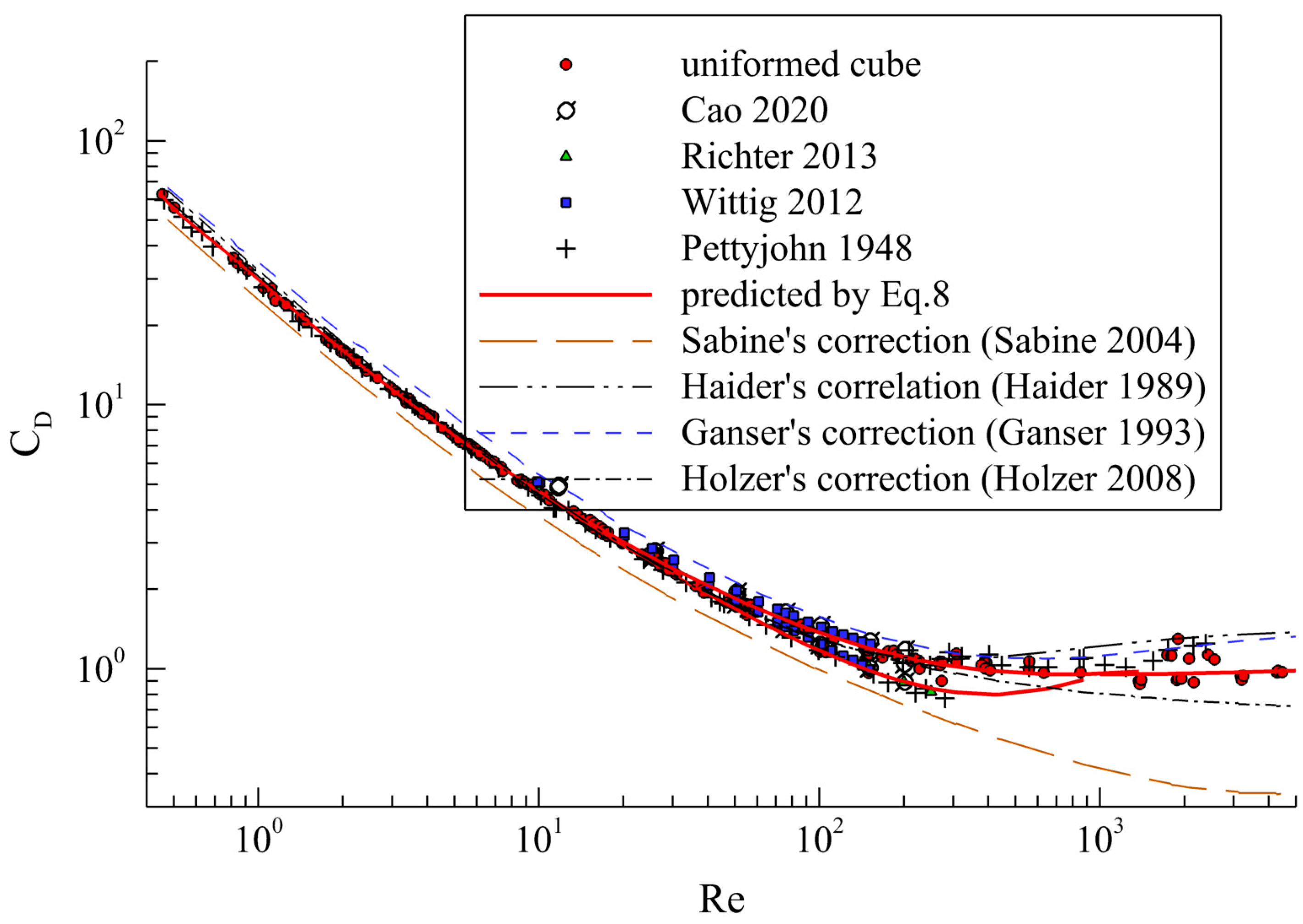
4.1. Behavior of Uniform Cube Drag Coefficient
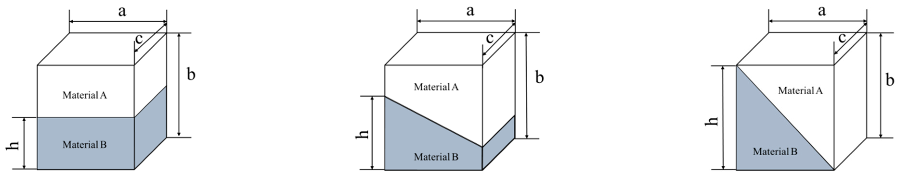
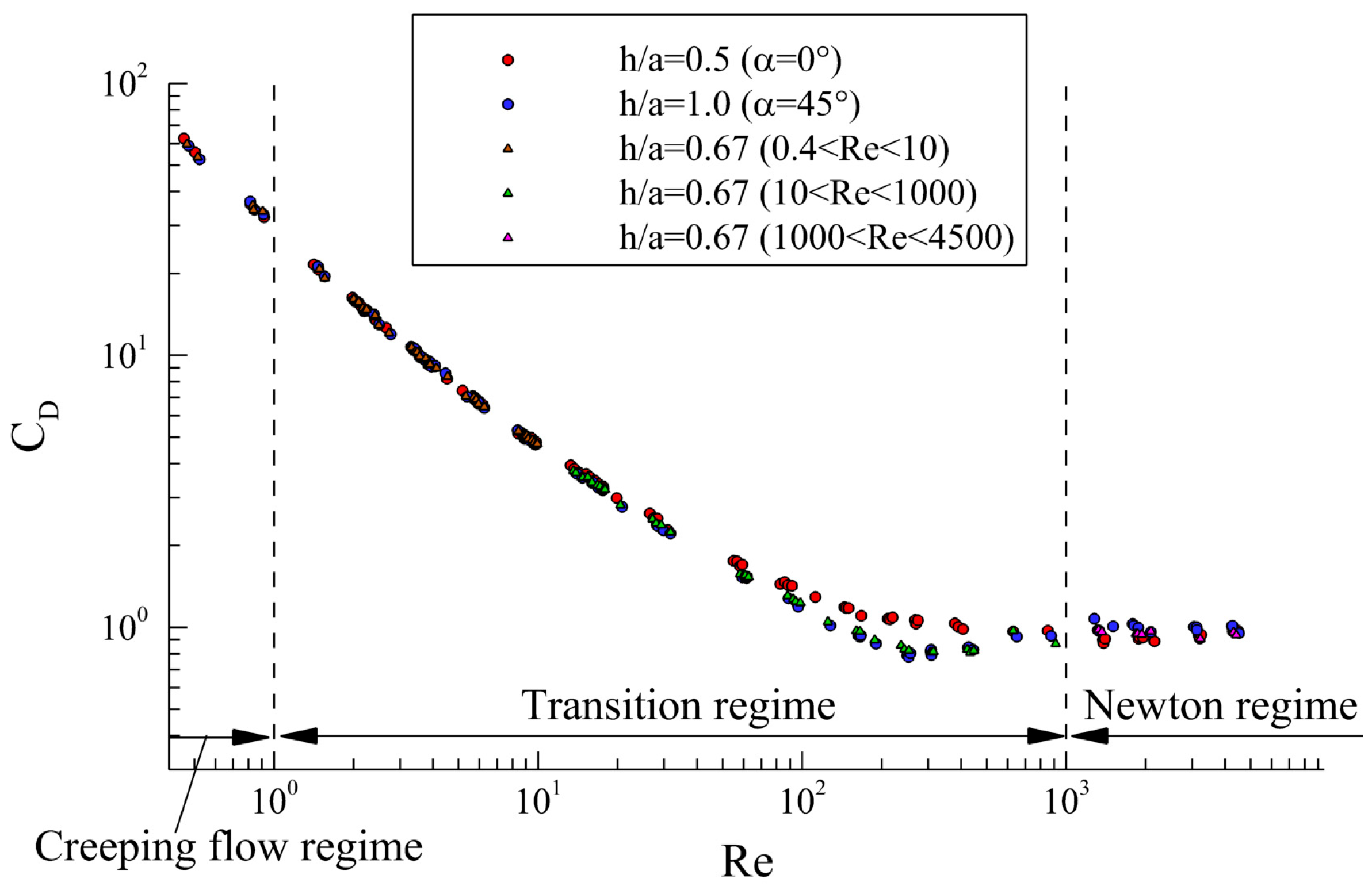
4.2. Behavior of the Spliced Cube Drag Coefficient
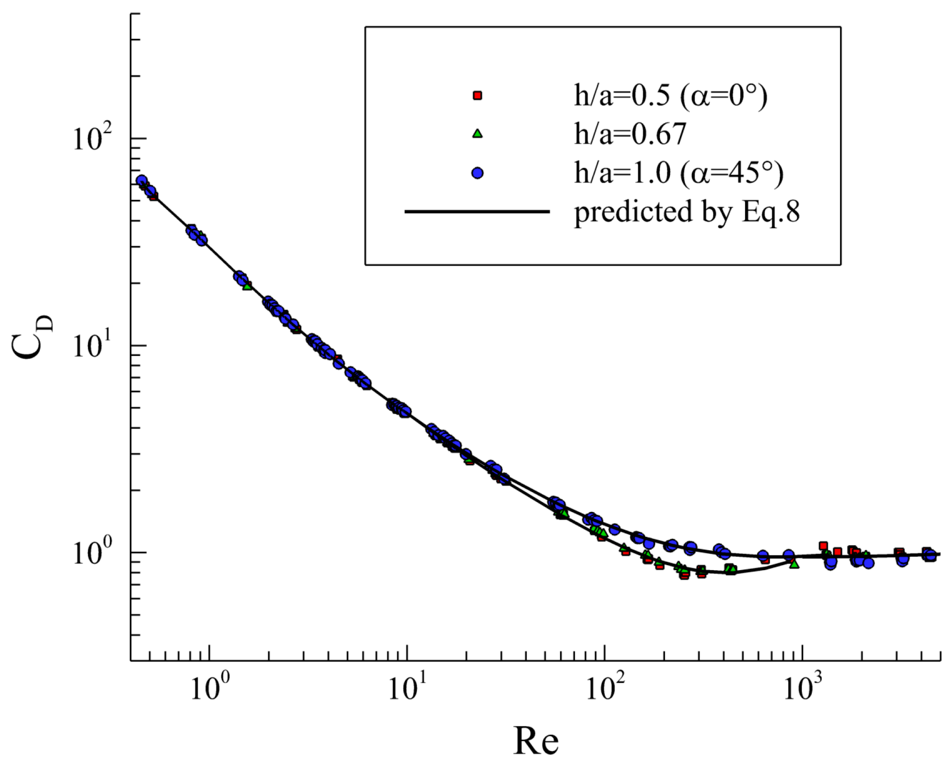
4.3. Universal Drag Model for the Cube
5. Conclusions
Author Contributions
Funding
Institutional Review Board Statement
Informed Consent Statement
Data Availability Statement
Conflicts of Interest
Nomenclature
| Re | particle Reynolds number |
| Cd | the drag coefficient |
| a,b,c | edge length of a cube |
| h | thickness of Material B |
| Vp | the volume of particle |
| dn | the volume-equivalent-sphere diameter |
| dA | the surface-equivalent sphere diameter |
| Pp | the projected perimeter of the particle in its direction of motion |
| A | maximum dimension of particle |
| B | intermediate dimension of particle |
| C | minimum dimension of particle |
| D | model parameters |
| ϕ | sphericity |
| ρp | the density of particle |
| ρf | the density of experimental liquids |
| the terminal velocity | |
| RMSE | The Root Mean Square Error |
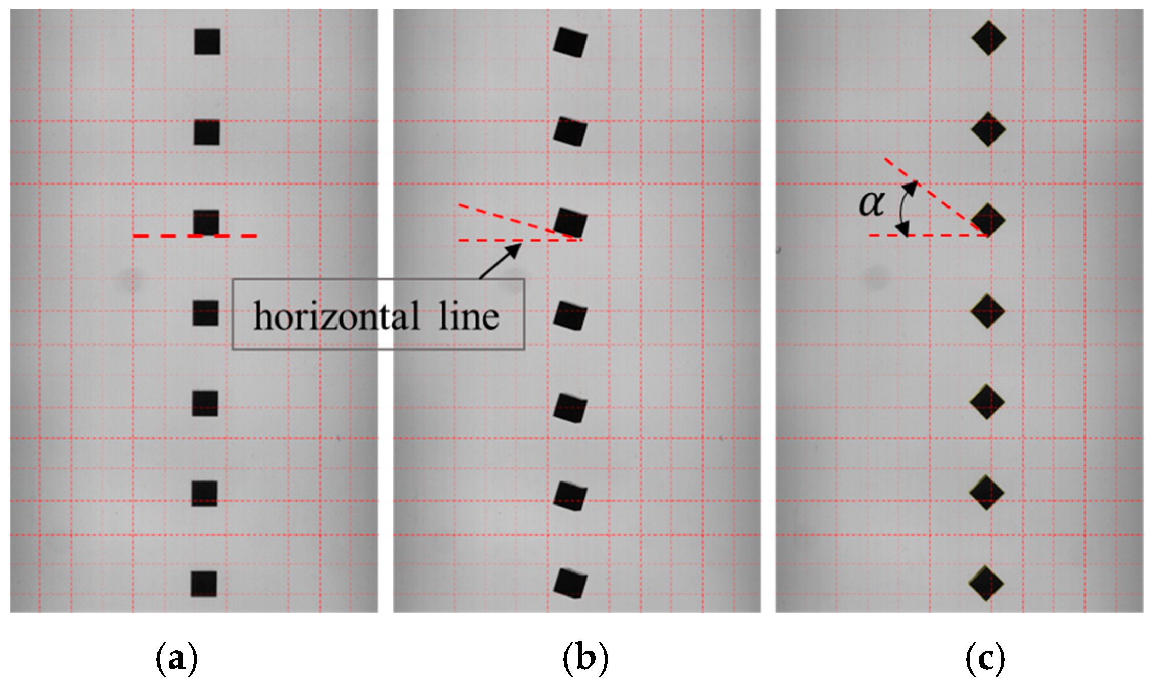
| α | the orientation angle |
| , | model parameters |
References
- Hamed, A.; Tabakoff, W.; Wenglarz, R. Erosion and Deposition in Turbomachinery. J. Propuls. Power 2006, 22, 350–360. [Google Scholar] [CrossRef]
- Filippone, A.; Bojdo, N. Turboshaft engine air particle separation. Prog. Aerosp. Sci. 2010, 46, 224–245. [Google Scholar] [CrossRef]
- Bagheri, G.; Bonadonna, C. On the Drag of Freely Falling Non-Spherical Particles. Powder Technol. 2016, 301, 526–544. [Google Scholar] [CrossRef]
- Brown, P.P.; Lawler, D.F. Sphere drag and settling velocity revisited. J. Environ. Eng.-ASCE 2003, 129, 222–231. [Google Scholar] [CrossRef]
- Turton, R.; Levenspiel, O. A short note on the drag correlation for spheres. Powder Technol. 1986, 47, 83–86. [Google Scholar] [CrossRef]
- Concha, F.; Barrientos, A. Settling velocities of particulate systems, 3. Power-series expansion for the drag coefficient of a sphere and prediction of the settling velocity. Int. J. Miner. Process. 1982, 9, 167–172. [Google Scholar] [CrossRef]
- Almedeij, J. Drag coefficient of flow around a sphere: Matching asymptotically the wide trend. Powder Technol. 2008, 186, 218–223. [Google Scholar] [CrossRef]
- Cheng, N. Comparison of formulas for drag coefficient and settling velocity of spherical particles. Powder Technol. 2009, 189, 395–398. [Google Scholar] [CrossRef]
- Clift, R.; Grace, J.R.; Weber, M.E. Bubbles, Drops and Particles; Academic Press: New York. NY, USA, 1978. [Google Scholar]
- Cao, Z.; Tafti, D.K.; Shahnam, M. Development of drag correlation for suspensions of ellipsoidal particles. Powder Technol. 2020, 369, 298–310. [Google Scholar] [CrossRef]
- Sabine, T.; Gay, M.; Michaelides, E.E. Drag coefficients of irregularly shaped particles. Powder Technol. 2004, 139, 21–32. [Google Scholar]
- Haider, A.; Levenspiel, O. Drag coefficient and terminal velocity of spherical and non-spherical particles. Powder Technol. 1989, 58, 63–70. [Google Scholar] [CrossRef]
- Swamee, P.K.; Ojha, C.S.P. Drag coefficient and fall velocity of nonspherical particles. J. Hydraul. Eng. 1991, 117, 660–667. [Google Scholar] [CrossRef]
- Ganser, G.H. A rational approach to drag prediction of spherical and nonspherical particles. Powder Technol. 1993, 77, 143–152. [Google Scholar] [CrossRef]
- Chien, S.F. Settling velocity of irregularly shaped particles. SPE Drill. Complet. 1994, 9, 281–289. [Google Scholar] [CrossRef]
- Yow, H.N.; Pitt, M.J.; Salman, A.D. Drag correlations for particles of regular shape. Adv. Powder Technol. 2005, 16, 363–372. [Google Scholar] [CrossRef]
- Hölzer, A.; Sommerfeld, M. New simple correlation formula for the drag coefficient of non-spherical particles. Powder Technol. 2008, 184, 361–365. [Google Scholar] [CrossRef]
- Rosendahl, L. Using a multi-parameter particle shape description to predict the motion of non-spherical particle shapes in swirling flow. Appl. Math. Model. 2000, 24, 11–25. [Google Scholar] [CrossRef]
- Wang, J.; Qi, H.; Zhu, J. Experimental study of settling and drag on cuboids with square base. Particuology 2011, 9, 298–305. [Google Scholar] [CrossRef]
- Richter, A.; Nikrityuk, P.A. Drag forces and heat transfer coefficients for spherical, cuboidal and ellipsoidal particles in cross flow at sub-critical Reynolds numbers. Int. J. Heat Mass Transf. 2012, 55, 1343–1354. [Google Scholar] [CrossRef]
- Agarwal, N.; Chhabra, R.P. Settling velocity of cubes in Newtonian and Power law liquids. Powder Technol. 2007, 178, 17–21. [Google Scholar] [CrossRef]
- Delidis, P.; Stamatoudis, M. Comparison of the velocities and the wall effect between spheres and cubes in the accelerating region. Chem. Eng. Commun. 2009, 196, 841–853. [Google Scholar] [CrossRef]
- Richter, A.; Nikrityuk, P.A. New correlations for heat and fluid flow past ellipsoidal and cubic particles at different angles of attack. Powder Technol. 2013, 249, 463–474. [Google Scholar] [CrossRef]
- Miyamura, A.; Iwasaki, S.; Ishii, T. Experimental Wall Correction Factors of Single Solid Sphere in Triangular and Square Cylinders, and Parallel Plates. Int. J. Multiph. Flow 1981, 7, 41–46. [Google Scholar] [CrossRef]
- Wittig, K.; Richter, A.; Nikrityuk, P.A. Numerical Study of Heat and Fluid Flow Past a Cubical Particle at Sub-Critical Reynolds Numbers. In Proceedings of the ICHMT International Symposium on Advances in Computational Heat Transfer, Bath, UK, 1–5 July 2012. [Google Scholar]
- Pettyjohn, E.S.; Christiansen, E.R. Effect of particle shape on freesettling rates of isometric particles. Chem. Eng. Prog. 1948, 44, 157–172. [Google Scholar]


| Ref. | Prediction Model |
|---|---|
| Sabine et al. [11] | , where . |
| Haider and Levenspiel [12] | , |
| Swamee and Ojha [13] | , where . |
| , | |
| Ganser [14] | where for isometric particles. |
| for non-isometric particles. | |
| . | |
| Chien [15] | . |
| Yow et al. [16] | . |
| Hölzer and Sommerfeld [17] | . |
| Bagheri and Bonadonna [3] | , |
| where and is the same as the Ganser [14]. |
| No | (mm) | (mm) | (mm) | Material A | Material B | Particle Density (kg/m3) | Initial Released Angle | |
|---|---|---|---|---|---|---|---|---|
| 1 | 16.10 | 16.26 | 16.08 | 0.5 | PVC | aluminum | 1912.33 | 0° ± 1° |
| 2 | 16.08 | 15.98 | 15.90 | brass | 4624 | |||
| 3 | 16.08 | 16.28 | 16.10 | steel | 4394.15 | |||
| 4 | 16.24 | 16.24 | 16.20 | 0.67 | aluminum | 1894.18 | 20° ± 1° | |
| 5 | 16.04 | 16.26 | 15.92 | brass | 4543.91 | |||
| 6 | 16.10 | 16.34 | 16.20 | steel | 4370.69 | |||
| 7 | 16.40 | 16.38 | 16.20 | 1.0 | aluminum | 1877.60 | 45° ± 1° | |
| 8 | 16.30 | 16.36 | 16.00 | brass | 4534.20 | |||
| 9 | 16.50 | 16.60 | 16.30 | steel | 4199.51 | |||
| 10 | 19.92 | 19.96 | 20.10 | 0.5 | PVC | aluminum | 1887.18 | 0° ± 1° |
| 11 | 20.00 | 19.96 | 20.10 | brass | 4684.99 | |||
| 12 | 20.10 | 19.92 | 20.30 | steel | 4453.89 | |||
| 13 | 19.96 | 20.40 | 19.92 | 0.67 | aluminum | 1884.21 | 20° ± 1° | |
| 14 | 20.00 | 20.40 | 20.00 | brass | 4648.28 | |||
| 15 | 20.16 | 20.30 | 20.26 | steel | 4352.84 | |||
| 16 | 20.16 | 20.24 | 19.90 | 1.0 | aluminum | 1868.11 | 45° ± 1° | |
| 17 | 20.20 | 20.22 | 19.96 | brass | 4621.75 | |||
| 18 | 20.30 | 20.18 | 19.90 | steel | 4325.75 |
| No | R (mm) | Material | Particle Density (kg/m3) |
|---|---|---|---|
| 1 | 7.00 | Steel | 7730 |
| 2 | 12.70 | ||
| 3 | 14.30 | ||
| 4 | 11.99 | Brass | 8300 |
| Re | ||||||
|---|---|---|---|---|---|---|
| 0.4 < Re < 10 | −0.02 | −3.633 | 3.907 | 0.754 | −0.378 | |
| 10 < Re < 1 × 10³ | upper bound | 0.213 | 0.653 | 0.05 | 1.344 | 152.85 |
| (α = 45°) | ||||||
| lower bound | 0.249 | 0.586 | 0.06 | 1.416 | 818.921 | |
| (α = 0°) | ||||||
| 1 × 10³ < Re < 4.516 × 10³ | 0.338 | 0.145 | 0.669 | 1.044 | −0.002 | |
Disclaimer/Publisher’s Note: The statements, opinions and data contained in all publications are solely those of the individual author(s) and contributor(s) and not of MDPI and/or the editor(s). MDPI and/or the editor(s) disclaim responsibility for any injury to people or property resulting from any ideas, methods, instructions or products referred to in the content. |
© 2025 by the authors. Licensee MDPI, Basel, Switzerland. This article is an open access article distributed under the terms and conditions of the Creative Commons Attribution (CC BY) license (https://creativecommons.org/licenses/by/4.0/).
Share and Cite
Wang, J.; Zhang, Y.; Miao, H.; Niu, J.; Cheng, D.; Chen, M. Experimental Investigation in Drag Coefficient of Cubes. Appl. Sci. 2025, 15, 7025. https://doi.org/10.3390/app15137025
Wang J, Zhang Y, Miao H, Niu J, Cheng D, Chen M. Experimental Investigation in Drag Coefficient of Cubes. Applied Sciences. 2025; 15(13):7025. https://doi.org/10.3390/app15137025
Chicago/Turabian StyleWang, Juanjuan, Yue Zhang, Huabing Miao, Jiajia Niu, Daishu Cheng, and Mingzhu Chen. 2025. "Experimental Investigation in Drag Coefficient of Cubes" Applied Sciences 15, no. 13: 7025. https://doi.org/10.3390/app15137025
APA StyleWang, J., Zhang, Y., Miao, H., Niu, J., Cheng, D., & Chen, M. (2025). Experimental Investigation in Drag Coefficient of Cubes. Applied Sciences, 15(13), 7025. https://doi.org/10.3390/app15137025