Author Contributions
Methodology, M.W. and C.C.; software, M.W., W.F. and C.C.; validation, M.W. and W.F.; formal analysis, M.W., W.F. and C.C.; data curation, M.W., W.F. and C.C.; writing—original draft preparation, M.W., W.F., X.L. and C.C.; writing—review and editing, M.W., W.F., X.L. and C.C.; visualization, M.W., X.L. and C.C.; supervision, M.W. and Y.L.; project administration, M.W. and Y.L.; and funding acquisition, M.W. and Y.L. All authors have read and agreed to the published version of the manuscript.
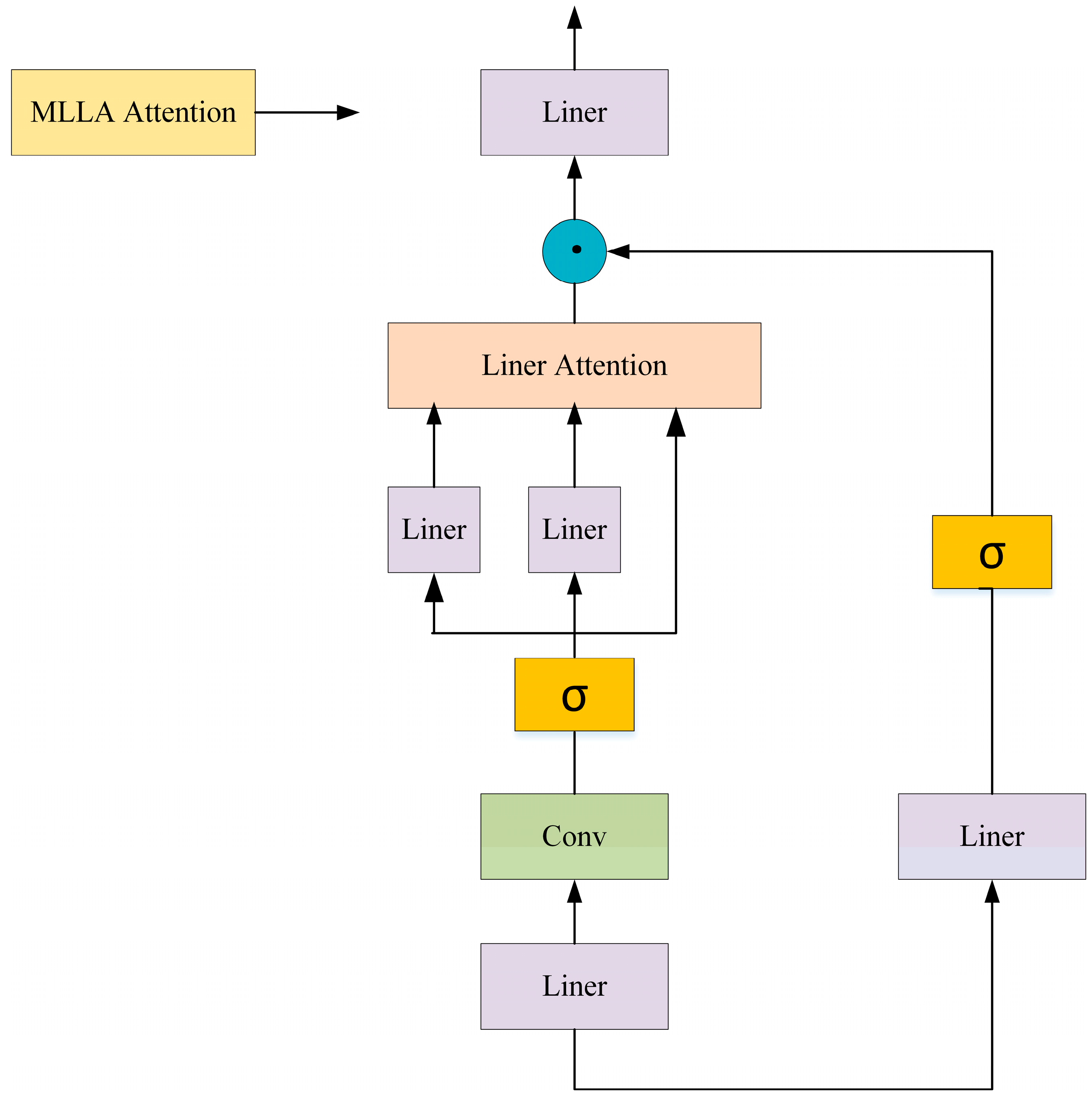
Figure 1.
MLLA structure.
Figure 1.
MLLA structure.
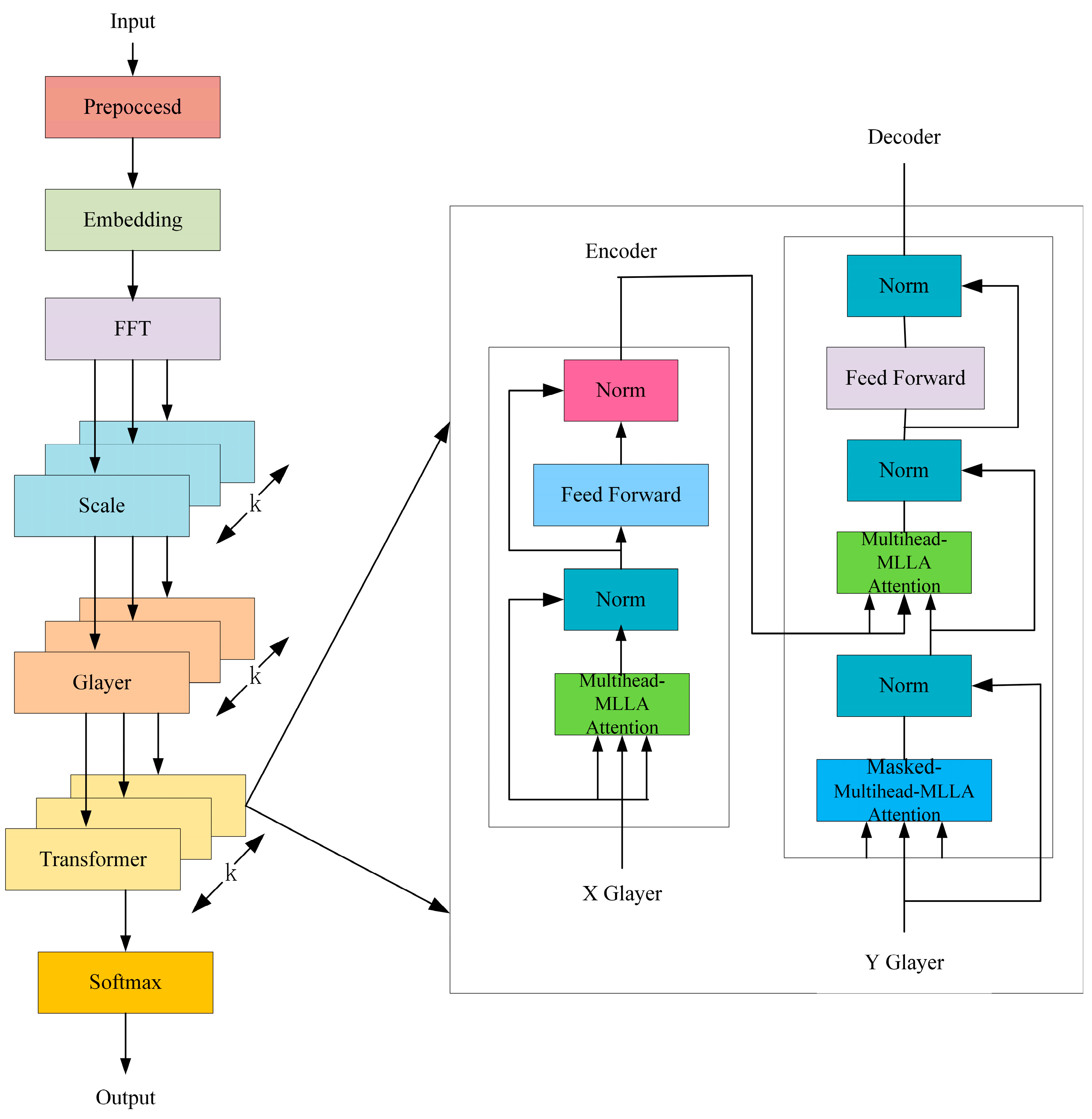
Figure 2.
MSGNet-MLLA-Transformer method flow.
Figure 2.
MSGNet-MLLA-Transformer method flow.
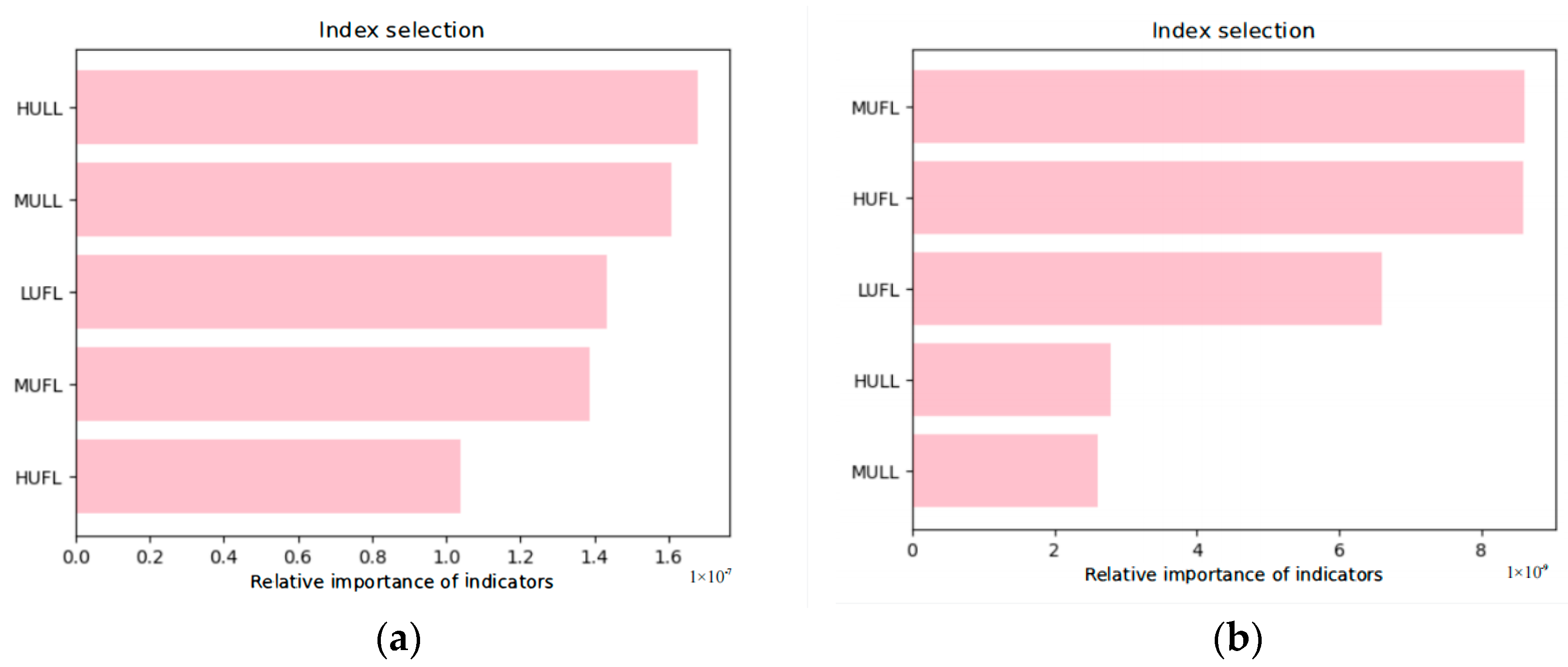
Figure 3.
Sequences left after random forest feature selection processing based on the ETTh1 and ETTm1 datasets, listed as (a) ETTh1 and (b) ETTm1.
Figure 3.
Sequences left after random forest feature selection processing based on the ETTh1 and ETTm1 datasets, listed as (a) ETTh1 and (b) ETTm1.
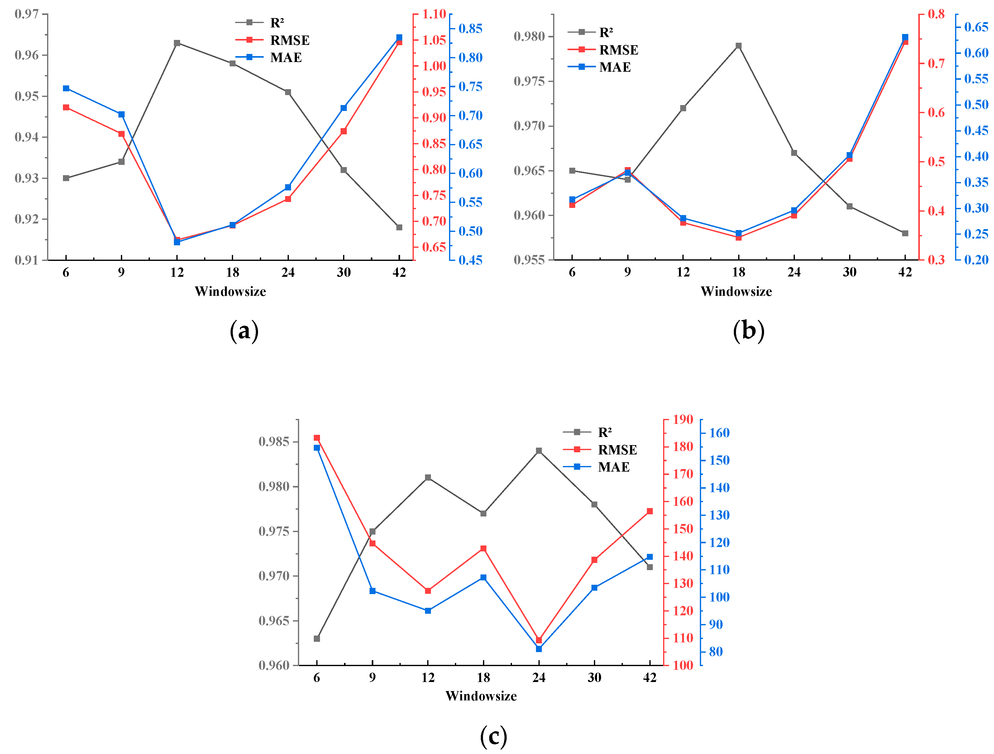
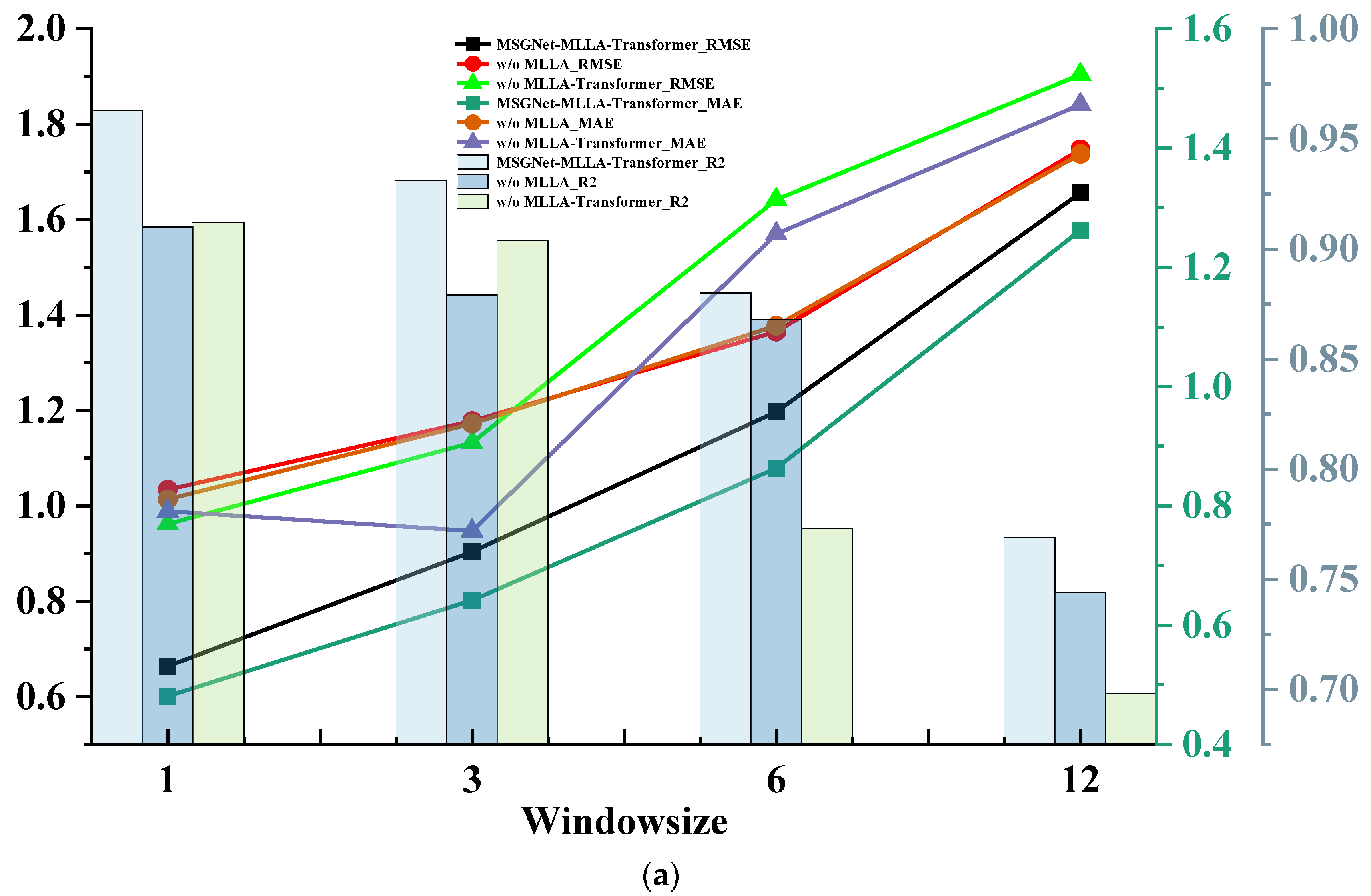
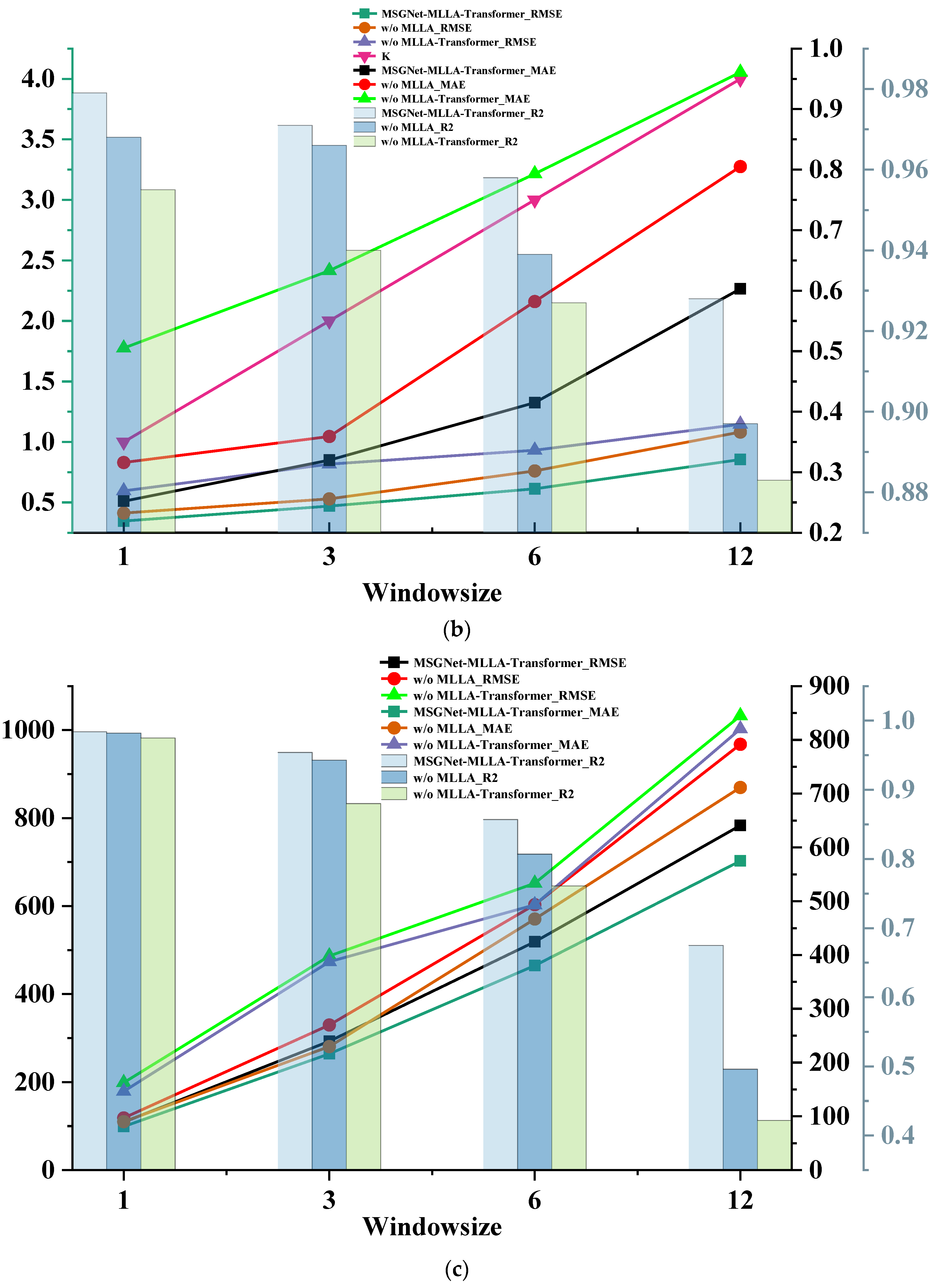
Figure 4.
Plot of time window metrics results on three datasets, listed as (a) ETTh1, (b) ETTm1, and (c) Australian electricity load.
Figure 4.
Plot of time window metrics results on three datasets, listed as (a) ETTh1, (b) ETTm1, and (c) Australian electricity load.
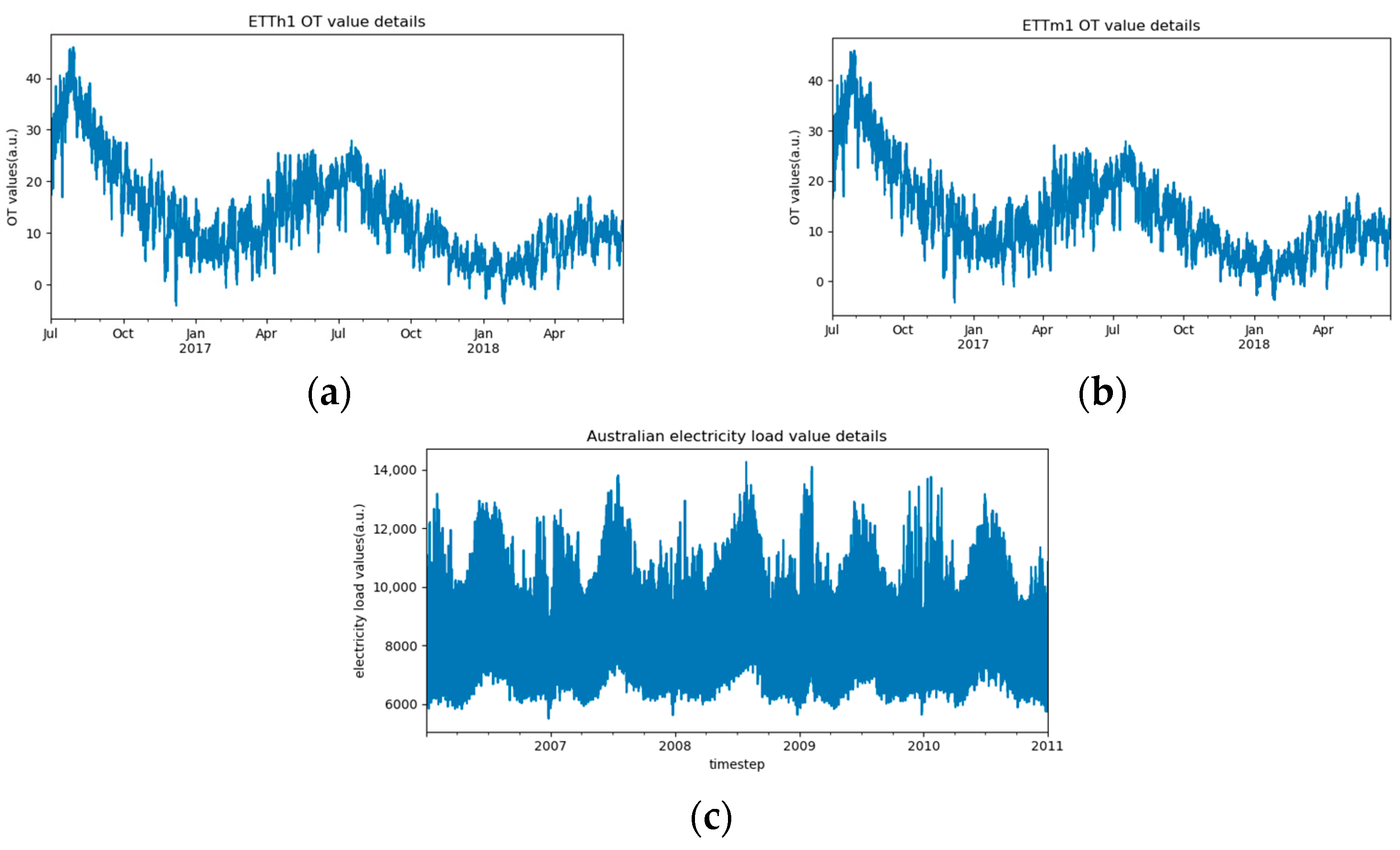
Figure 5.
Visualization of the target sequences of the three datasets, listed as (a) ETTh1; (b) ETTm1; and (c) Australian electricity load.
Figure 5.
Visualization of the target sequences of the three datasets, listed as (a) ETTh1; (b) ETTm1; and (c) Australian electricity load.
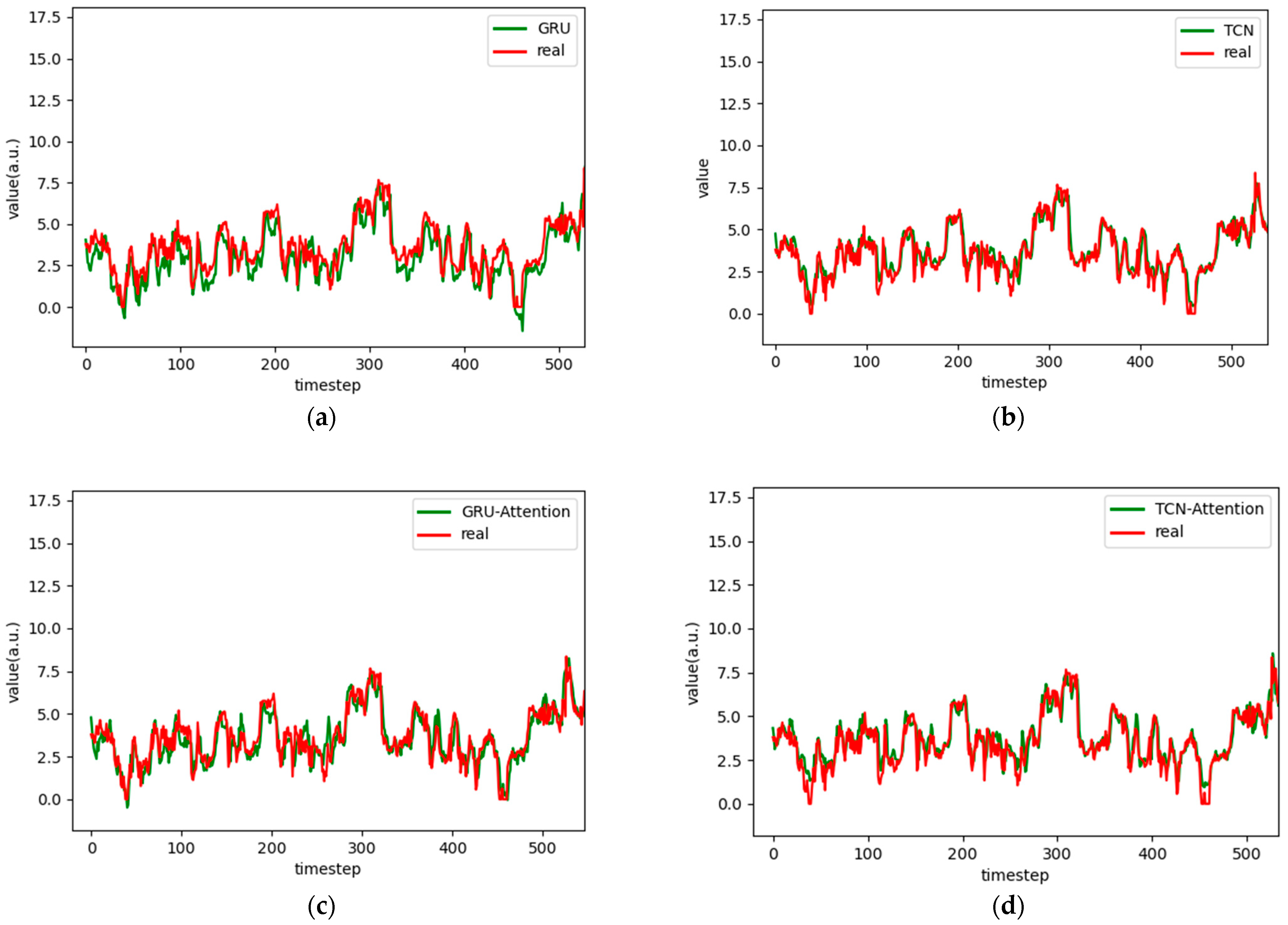
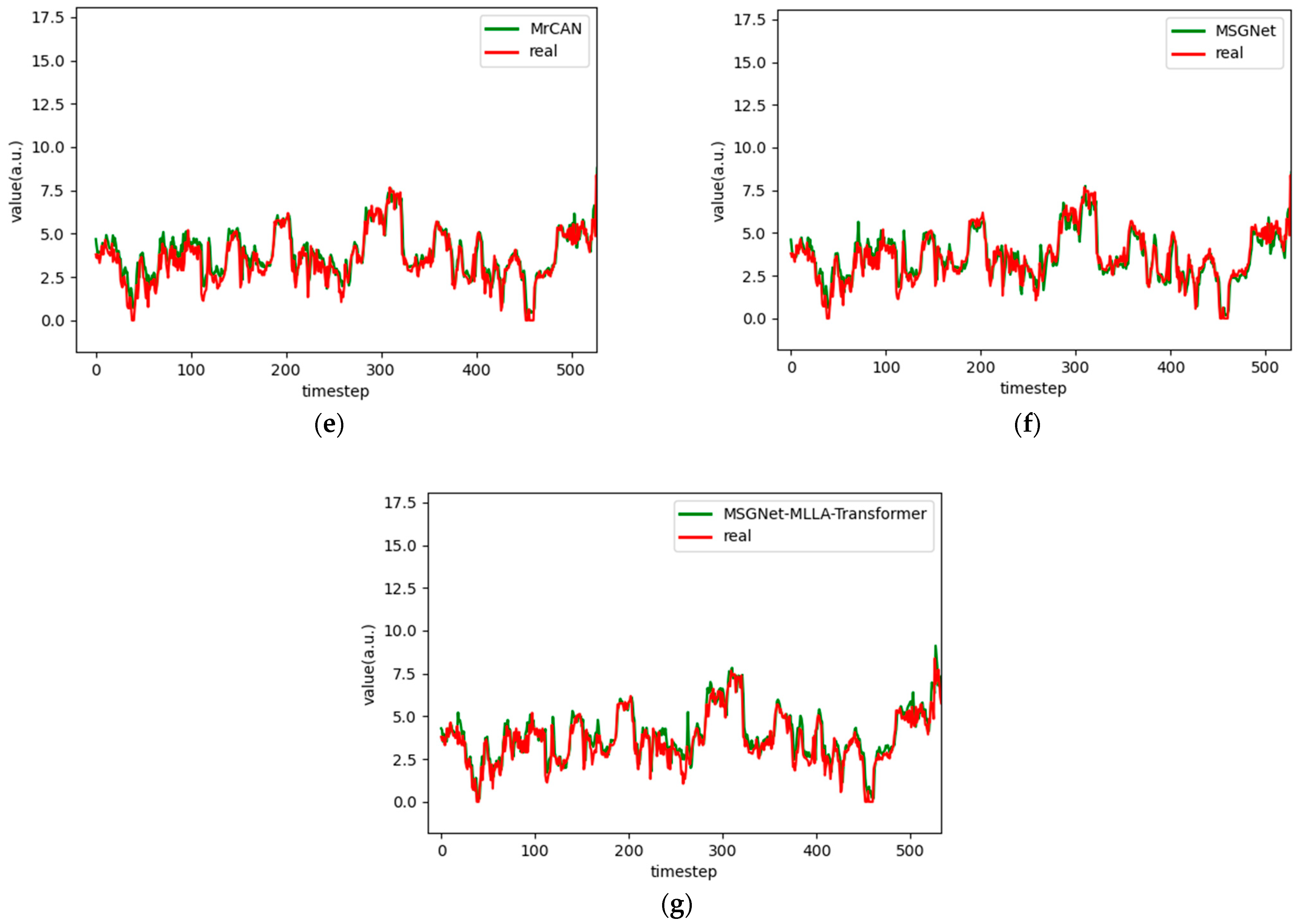
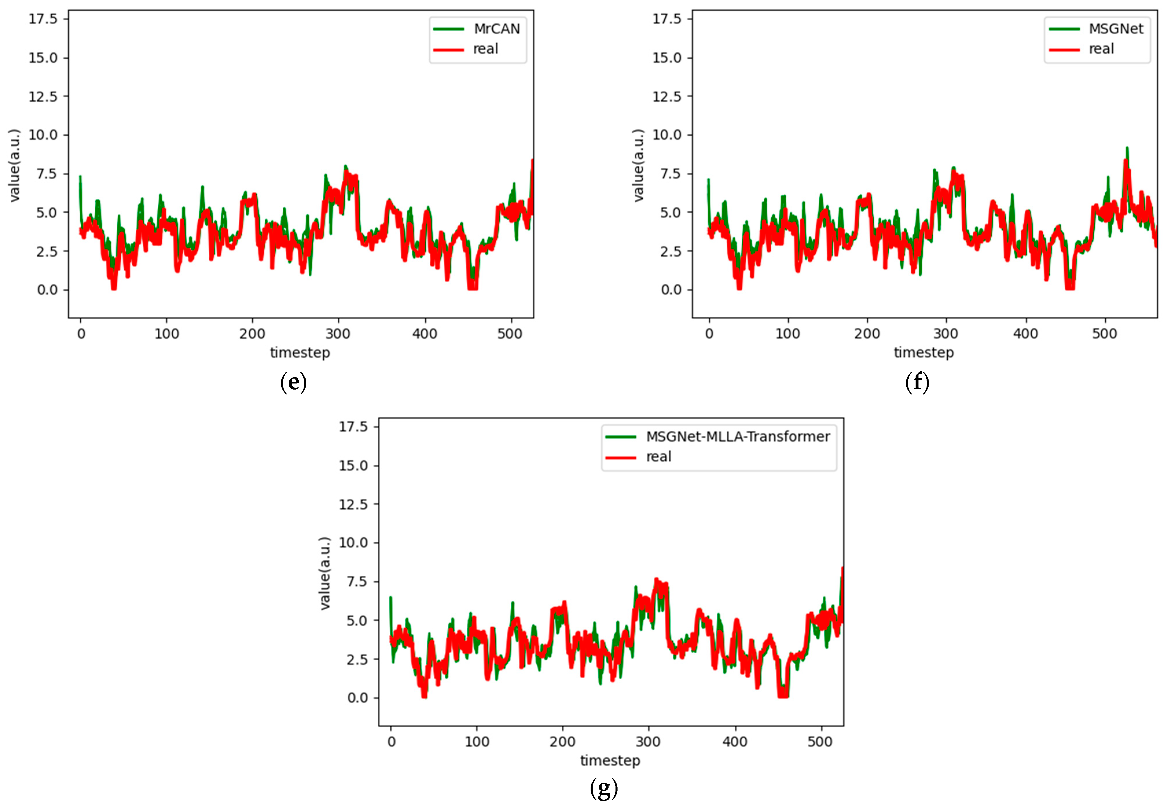
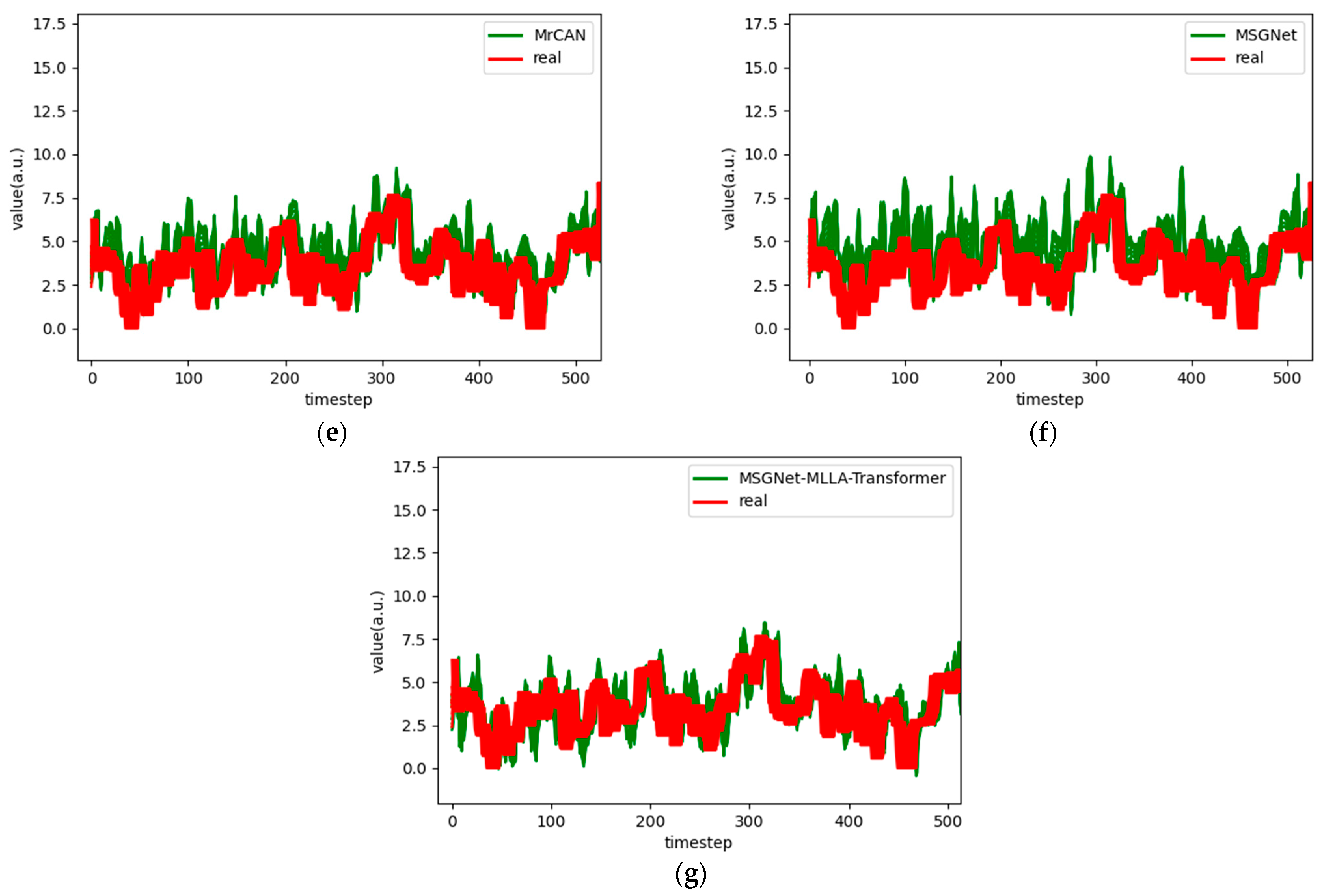
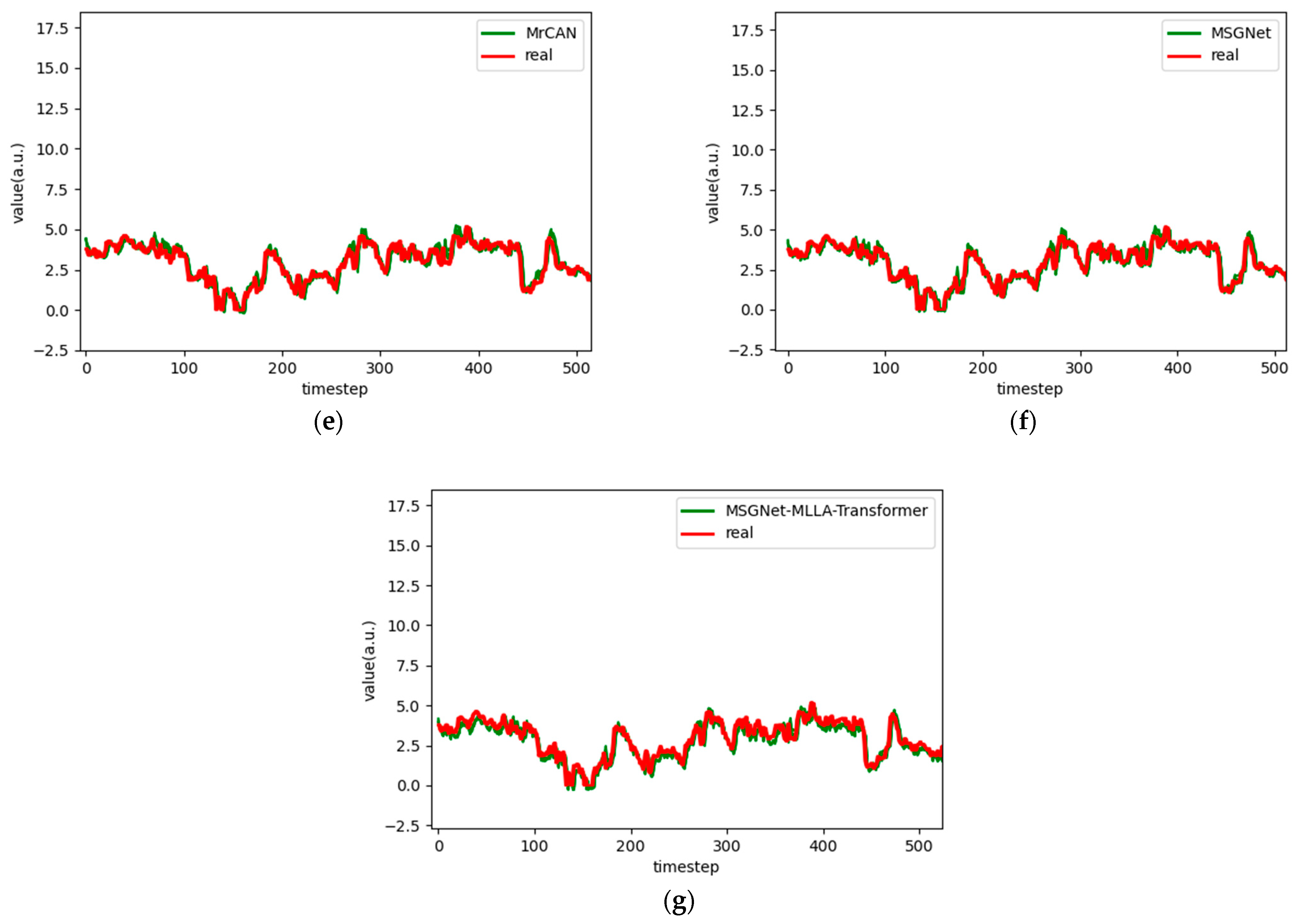
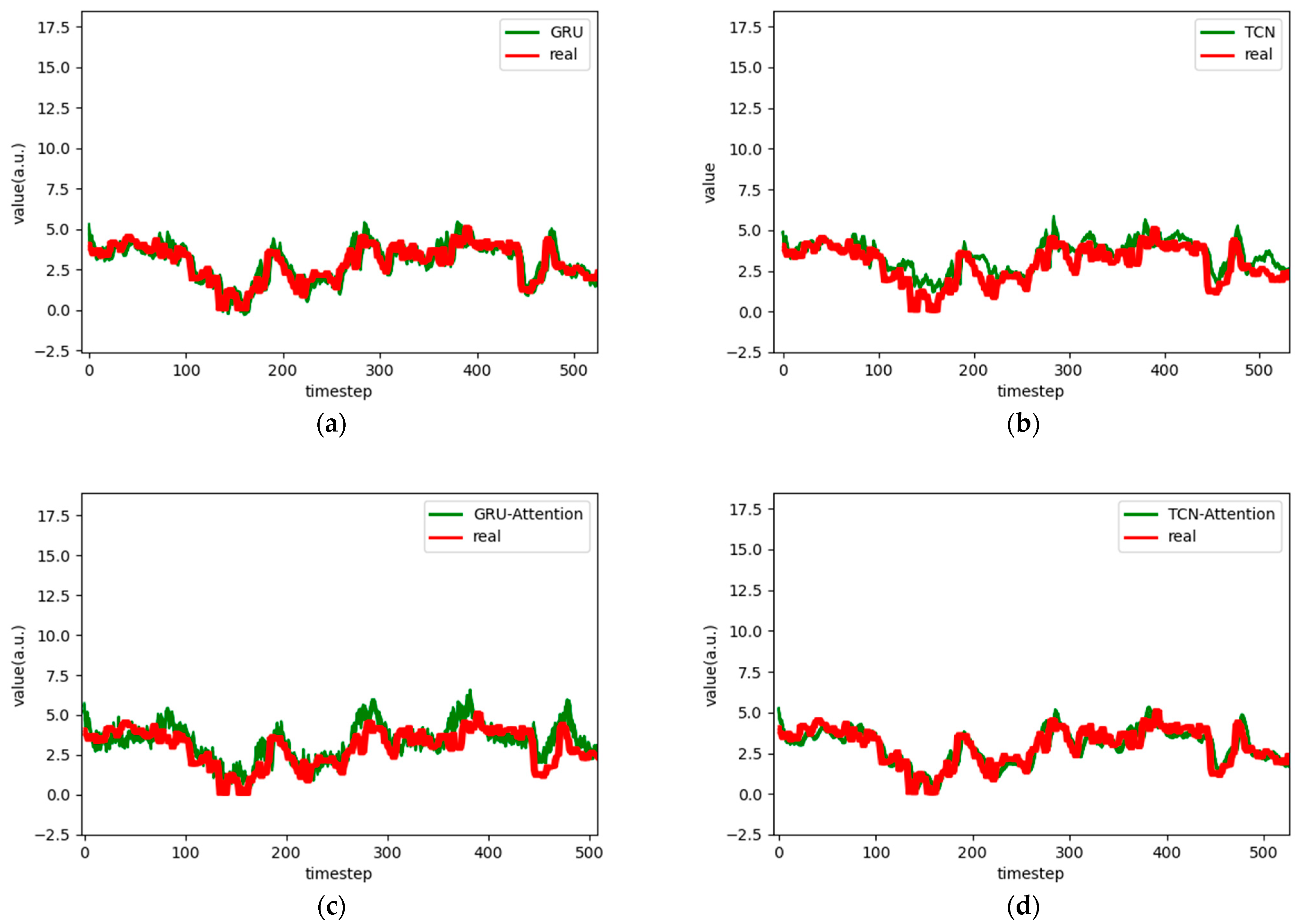
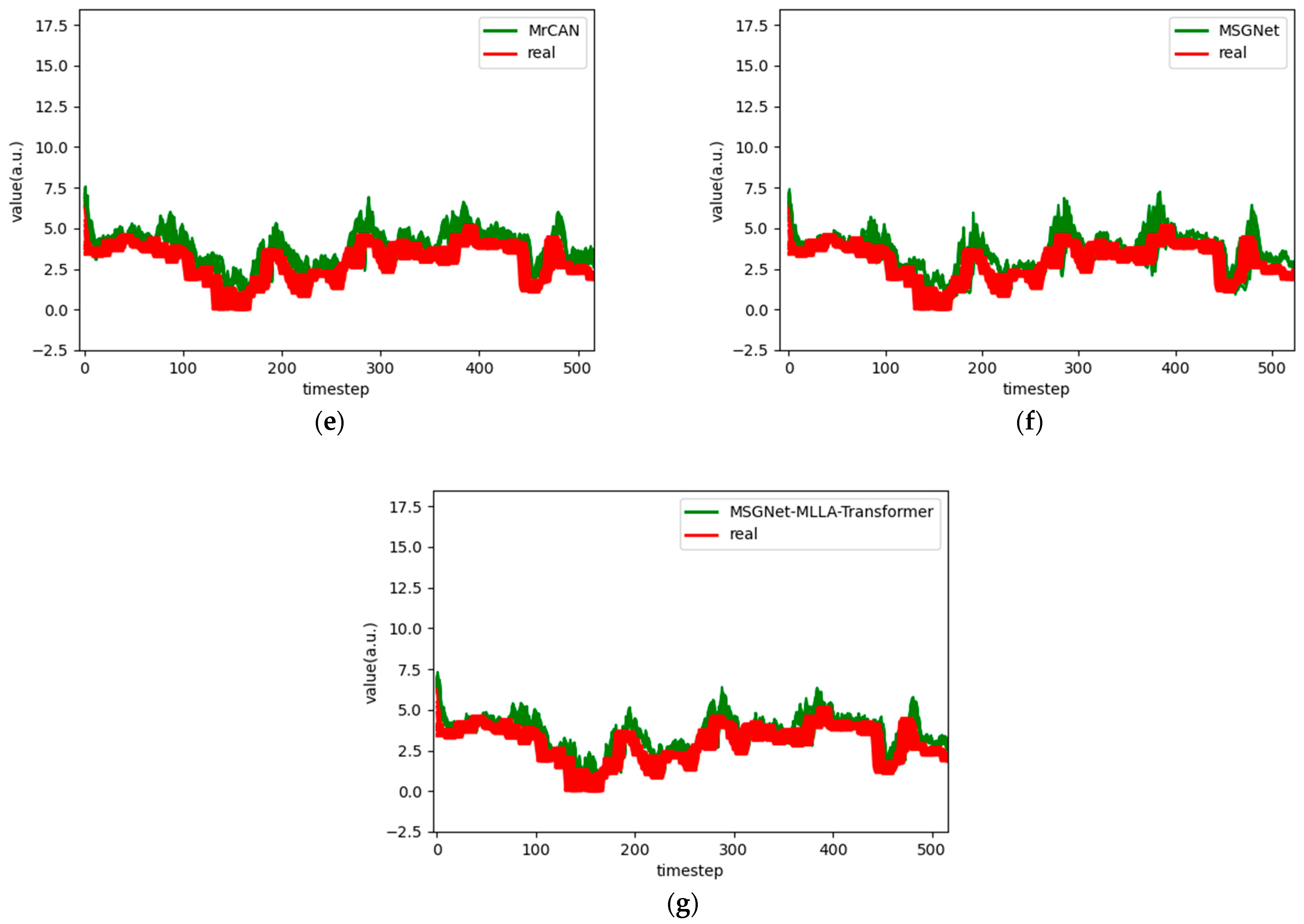
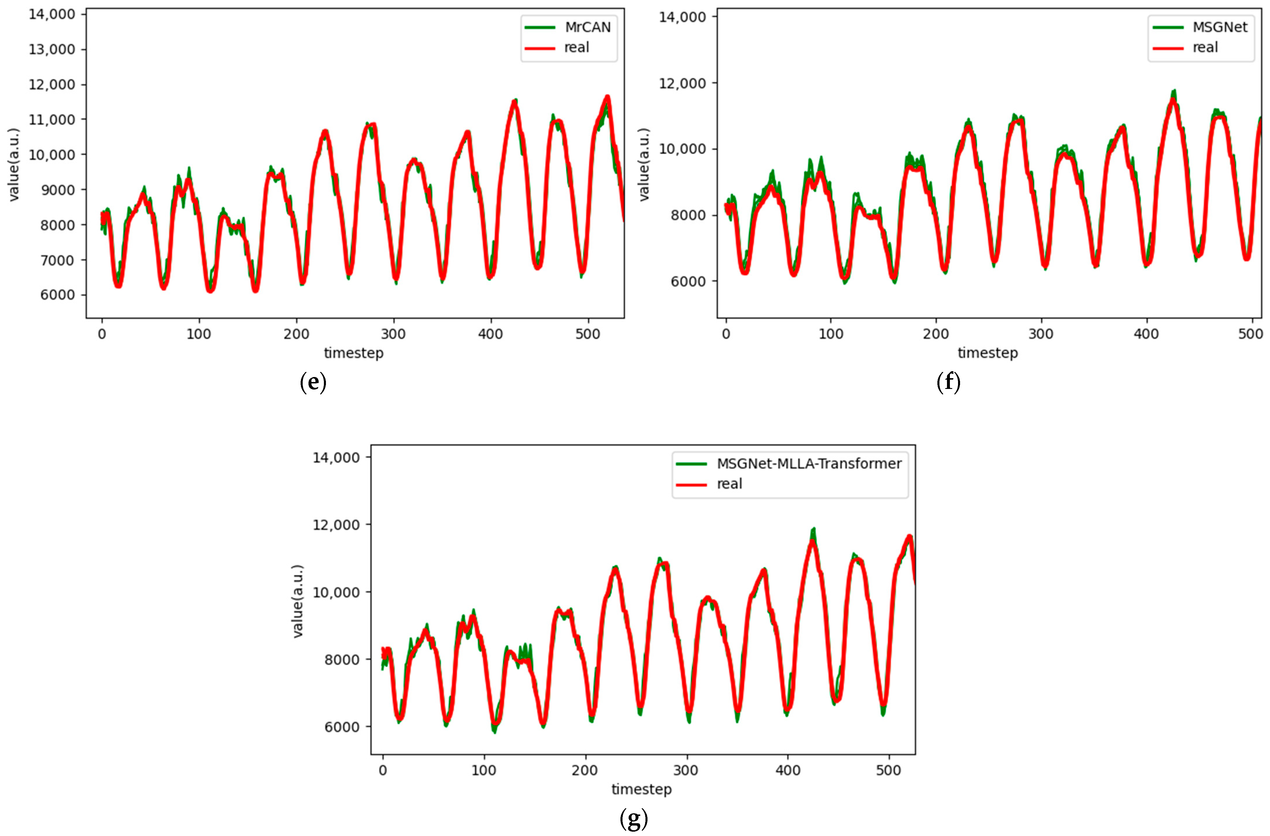
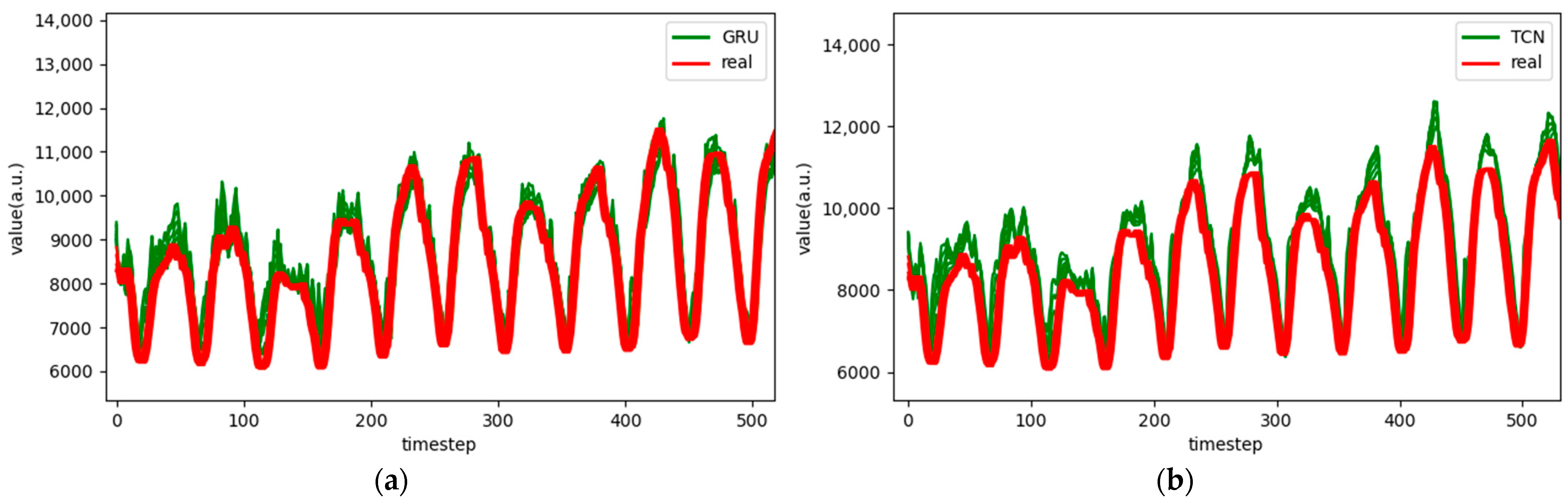
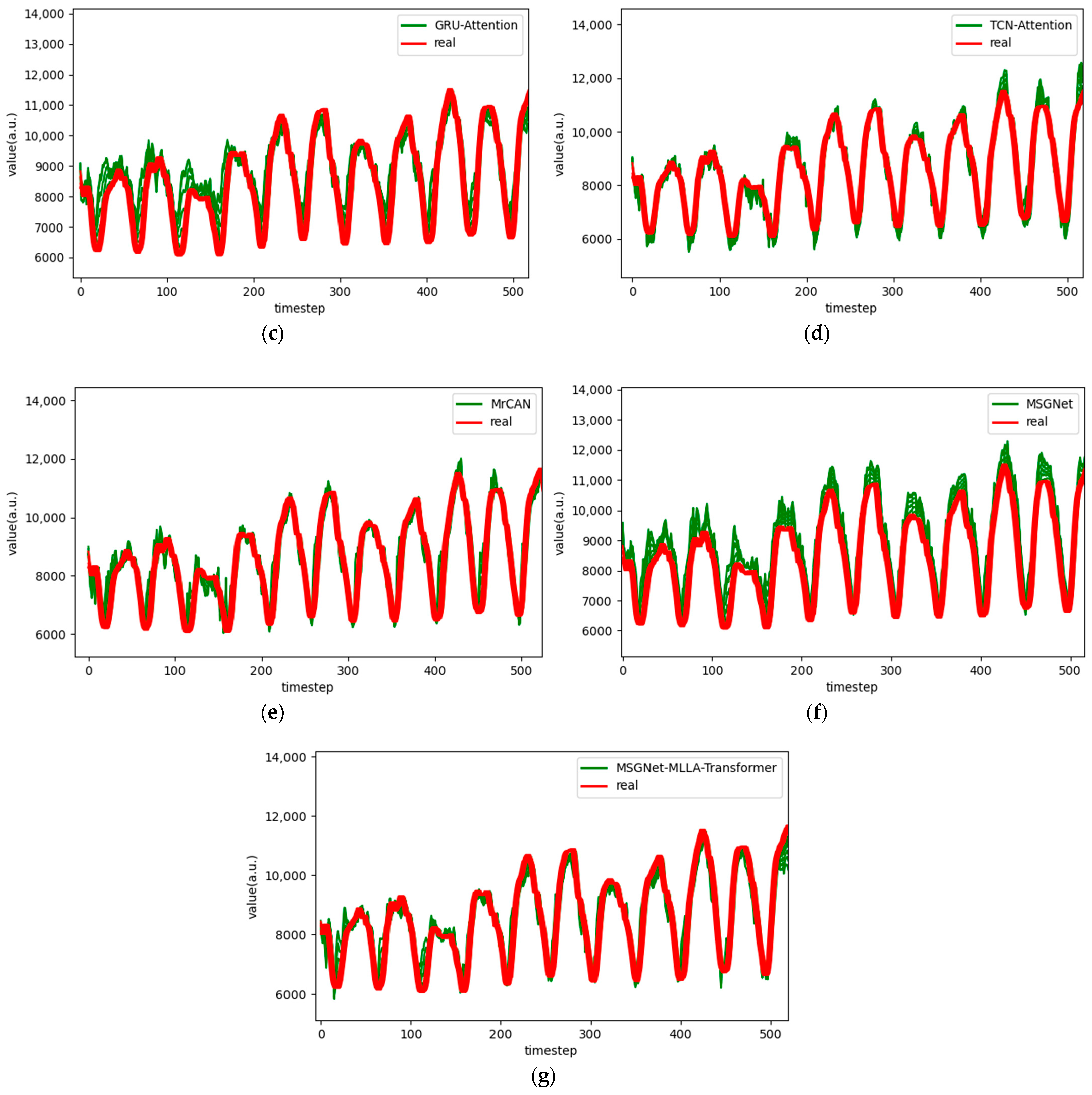
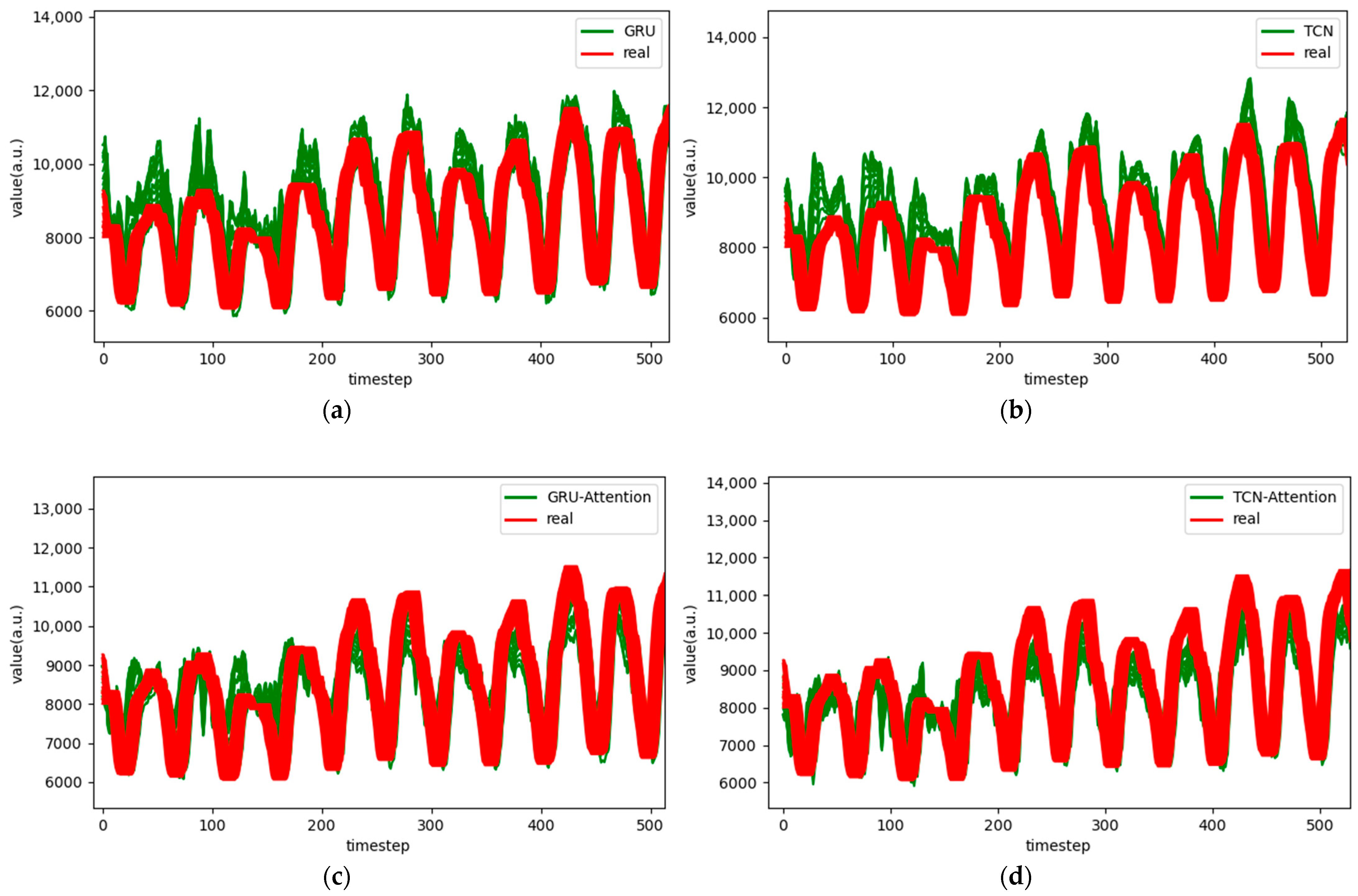
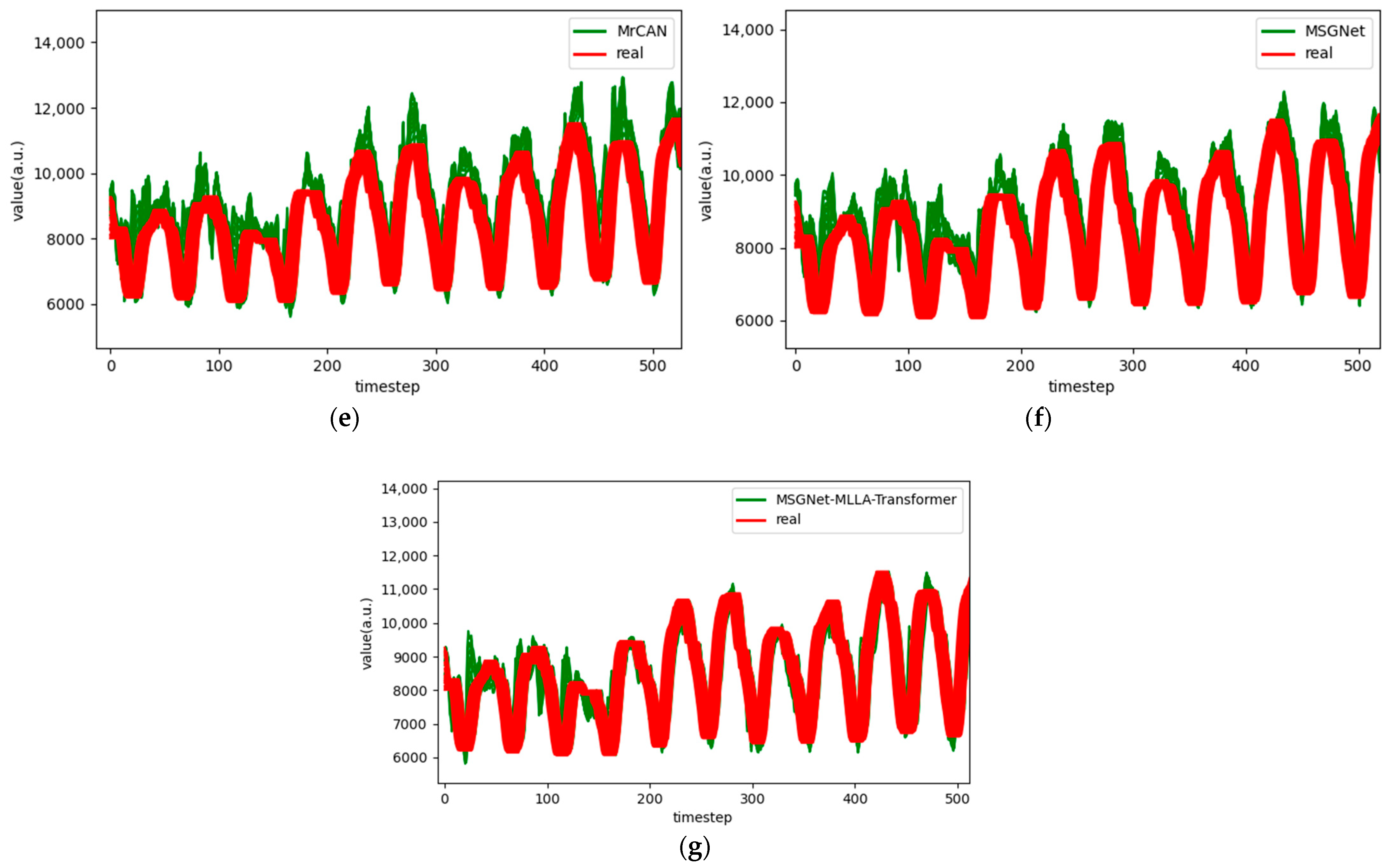
Figure 6.
Comparison chart fitting the 1-step prediction experimental model of the ETTh1 dataset, listed as (a) GRU; (b) TCN; (c) GRU-Attention; (d) TCN-Attention; (e) MrCAN; (f) MSGNet; and (g) Ours.
Figure 6.
Comparison chart fitting the 1-step prediction experimental model of the ETTh1 dataset, listed as (a) GRU; (b) TCN; (c) GRU-Attention; (d) TCN-Attention; (e) MrCAN; (f) MSGNet; and (g) Ours.
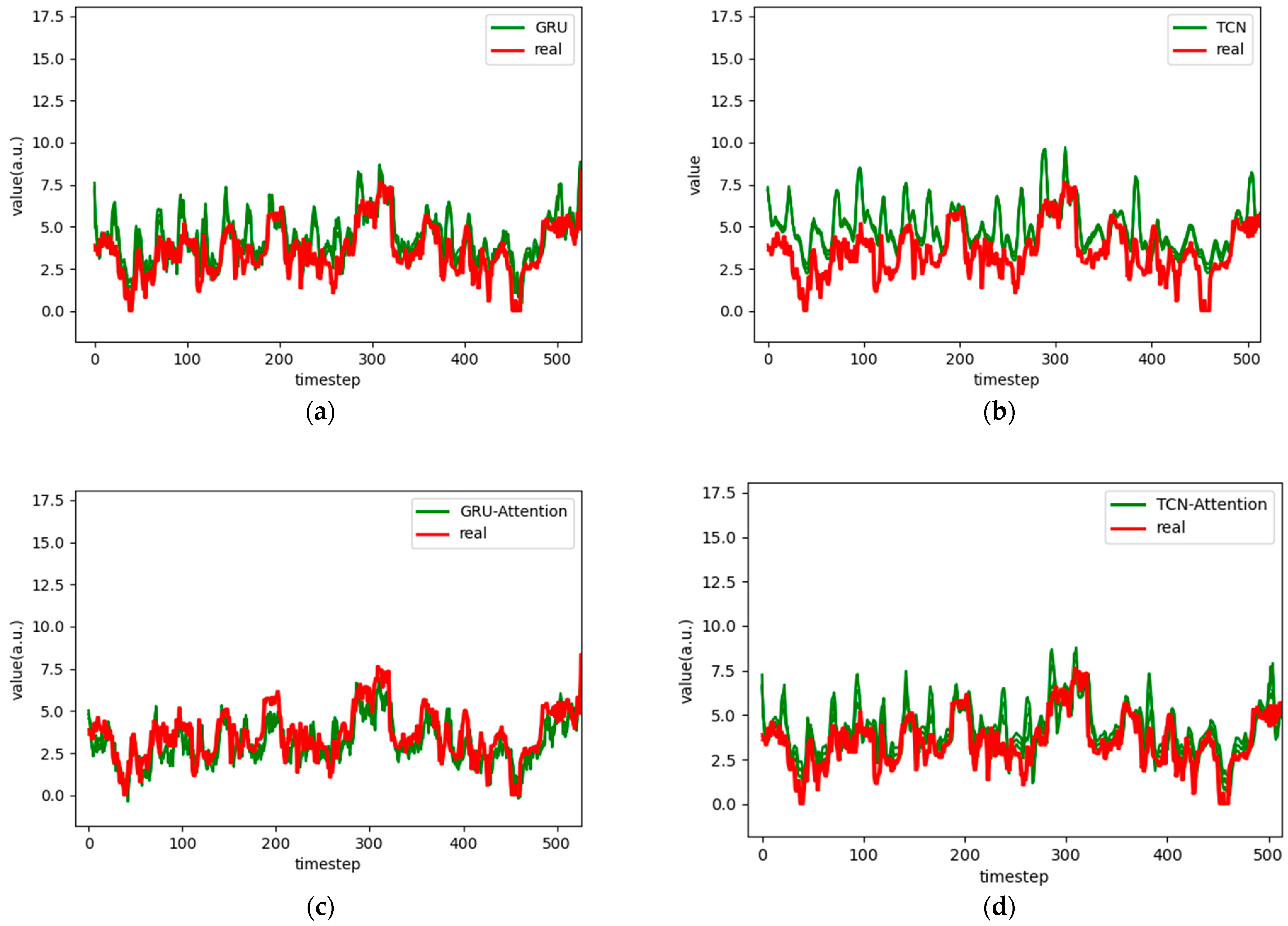
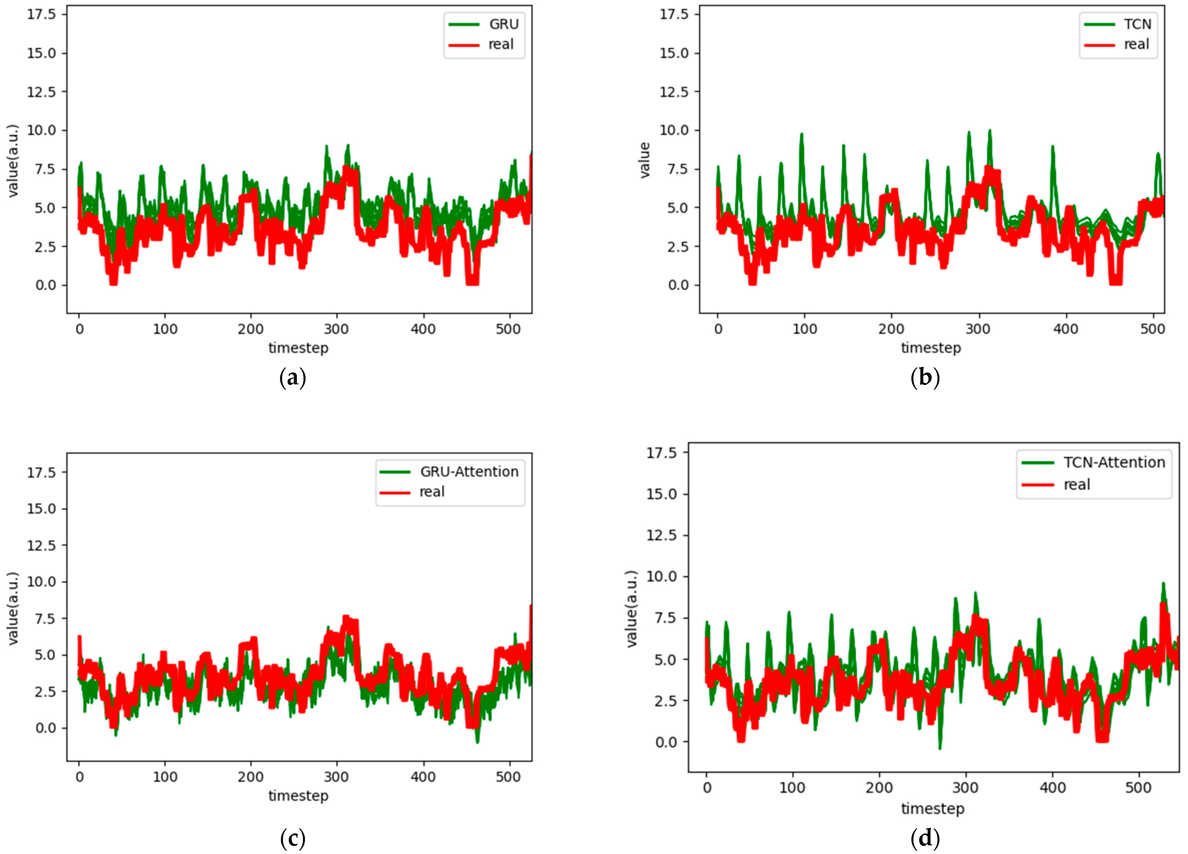
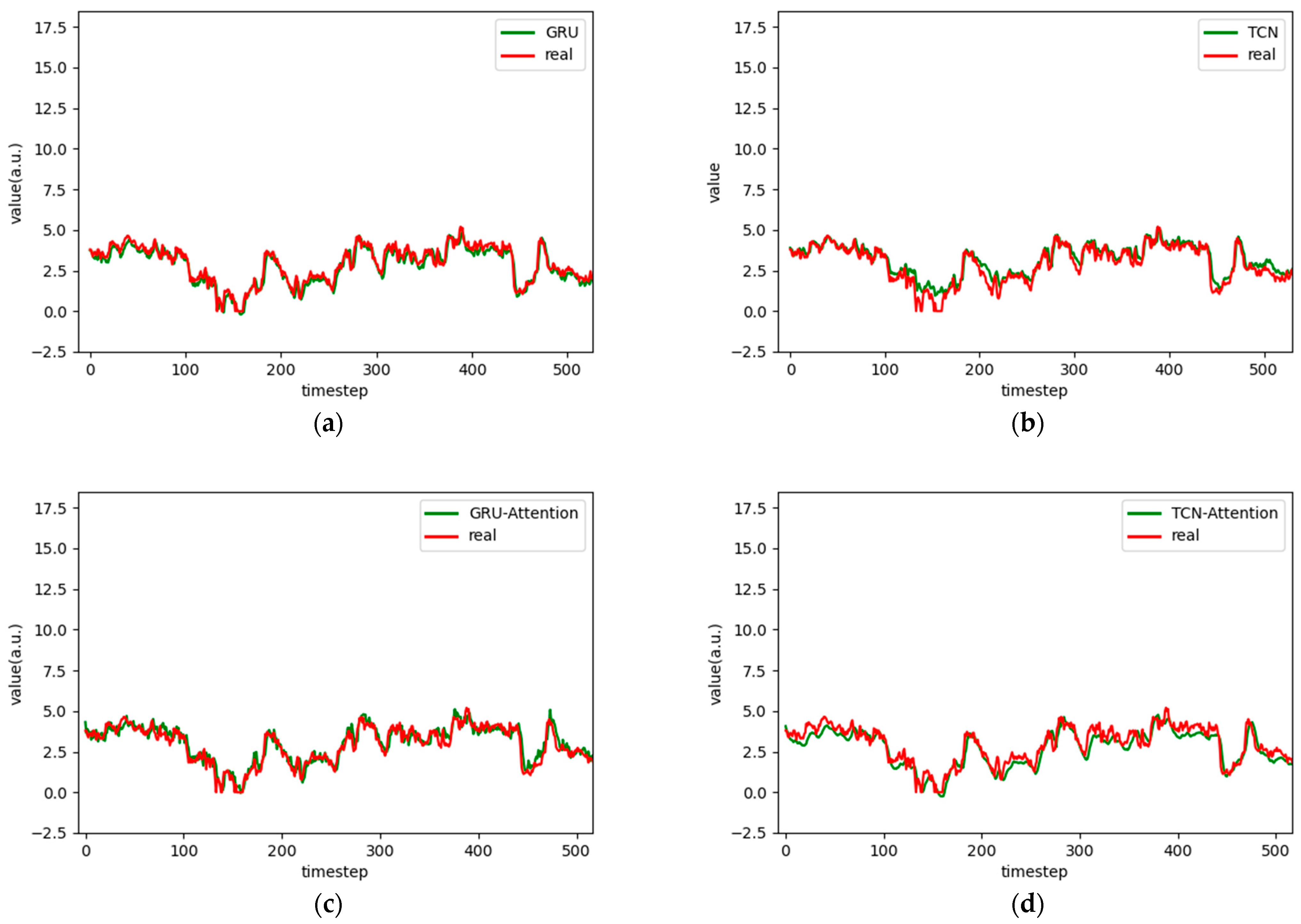
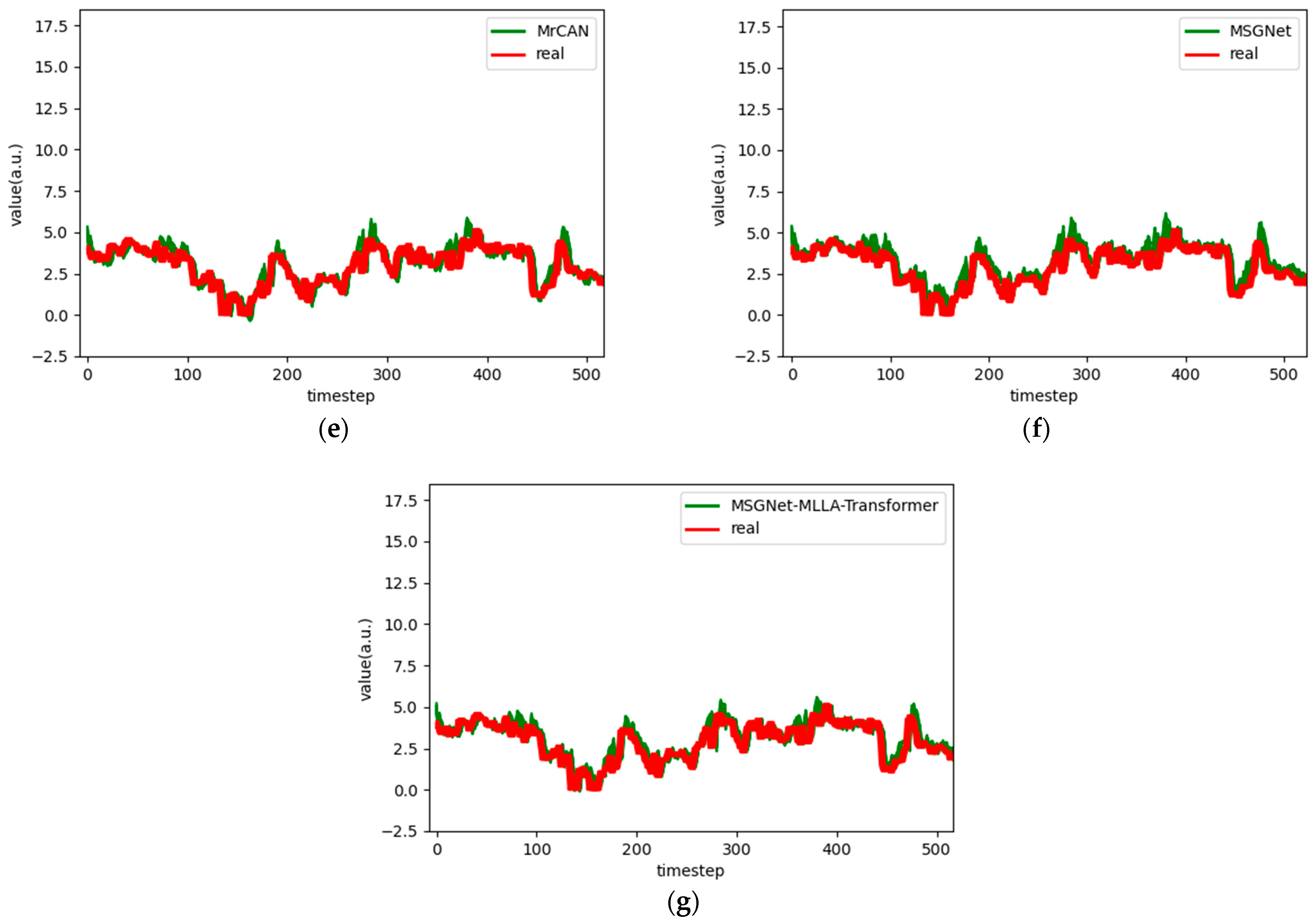
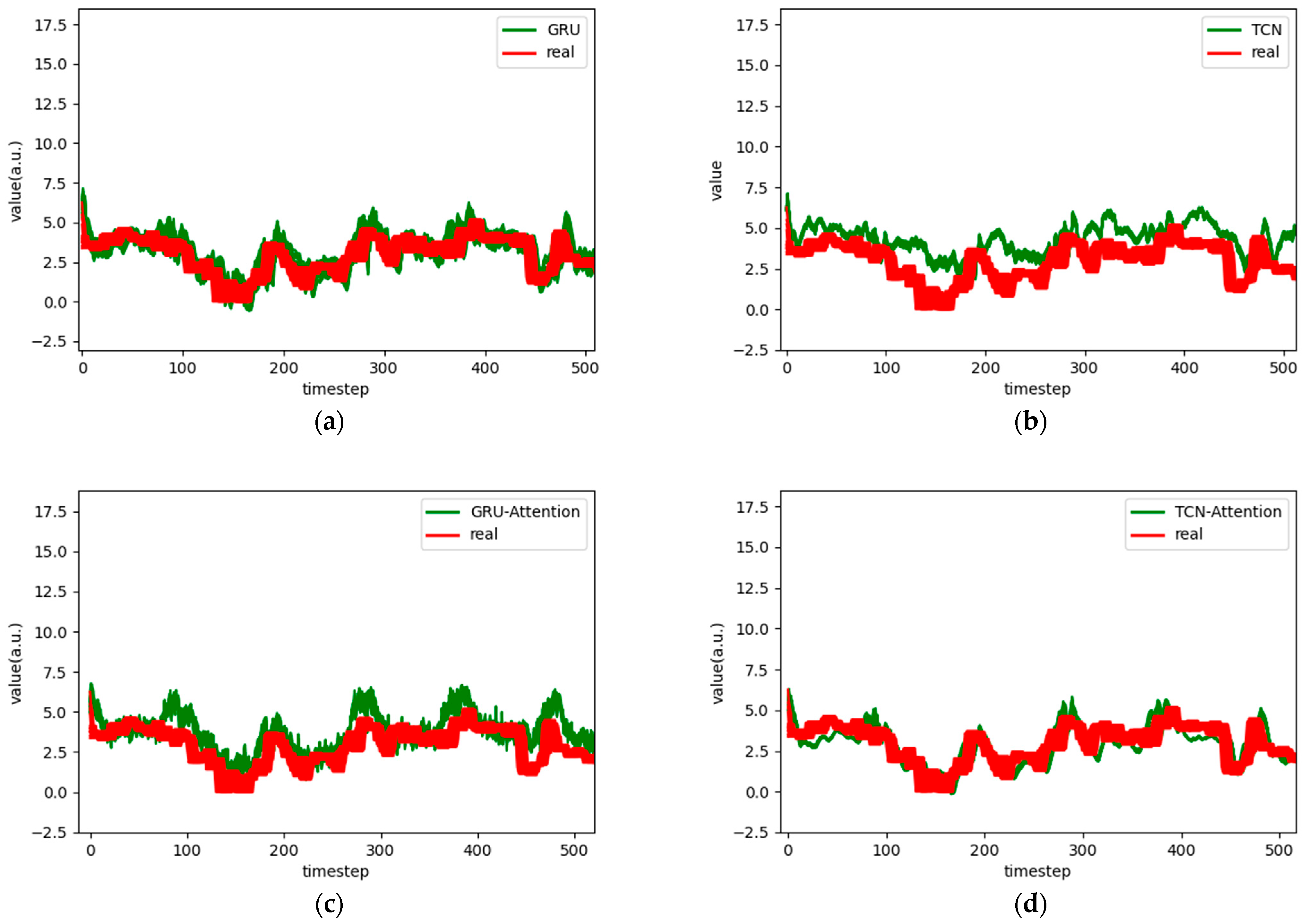
Figure 7.
Comparison chart fitting the 3-step prediction experimental model of the ETTh1 dataset, listed as (a) GRU; (b) TCN; (c) GRU-Attention; (d) TCN-Attention; (e) MrCAN; (f) MSGNet; and (g) Ours.
Figure 7.
Comparison chart fitting the 3-step prediction experimental model of the ETTh1 dataset, listed as (a) GRU; (b) TCN; (c) GRU-Attention; (d) TCN-Attention; (e) MrCAN; (f) MSGNet; and (g) Ours.
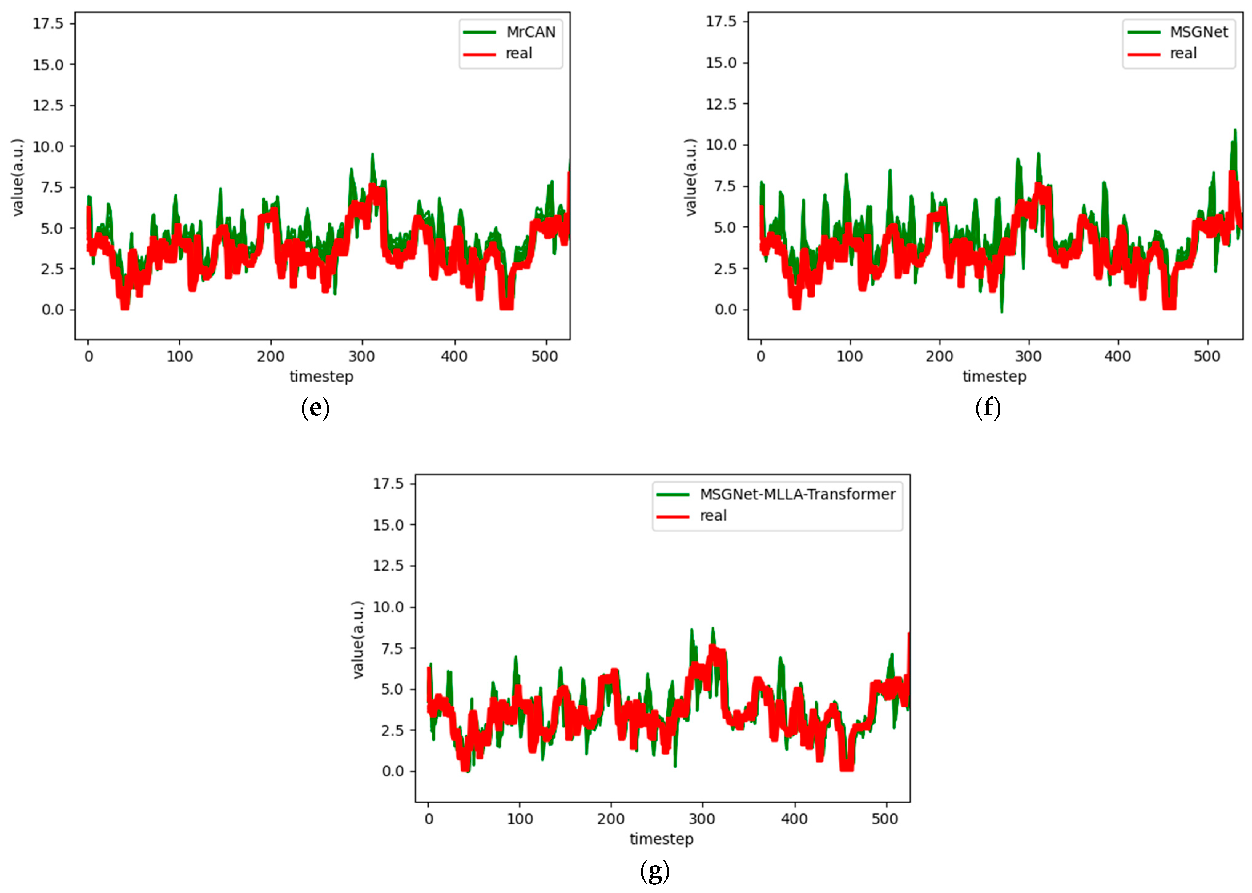
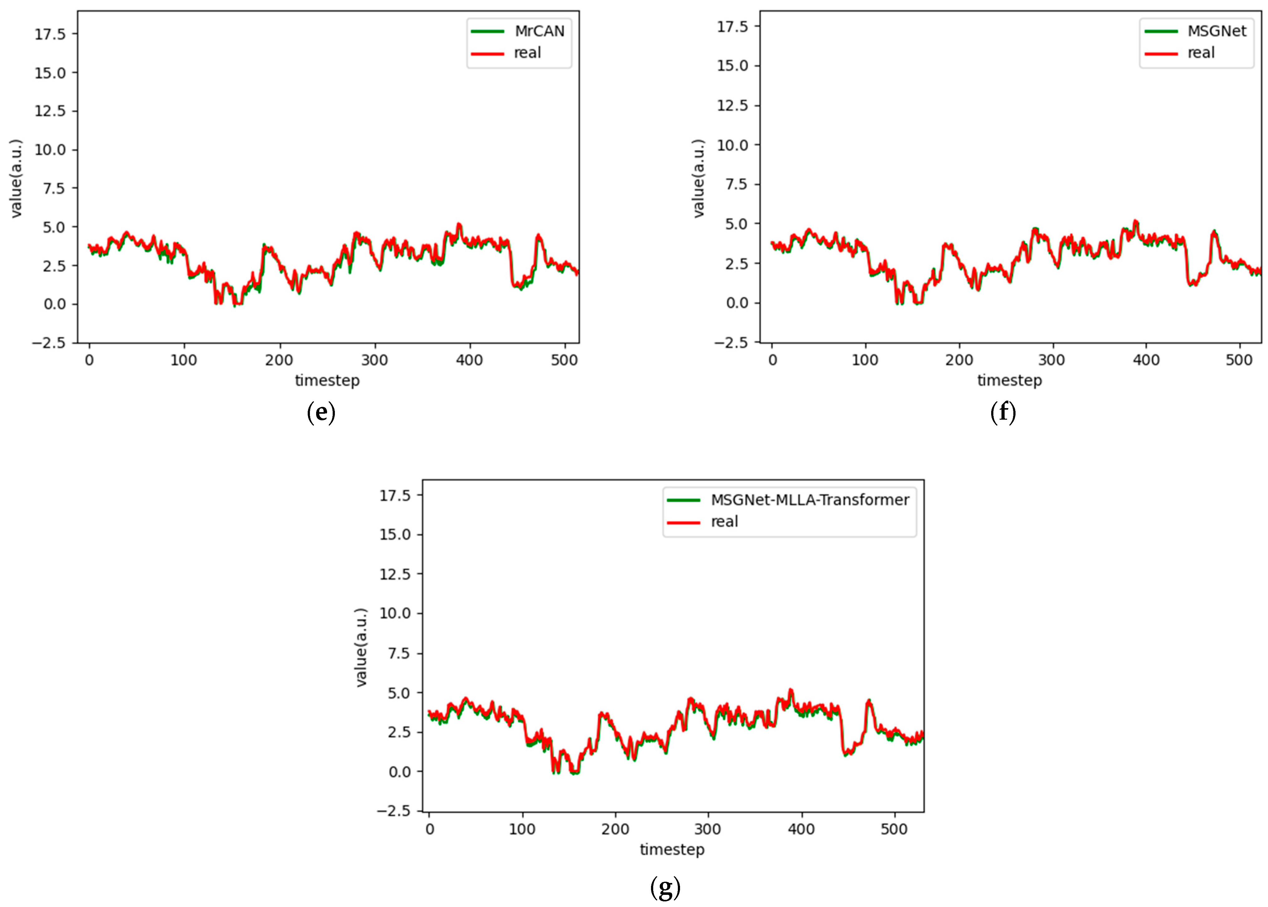
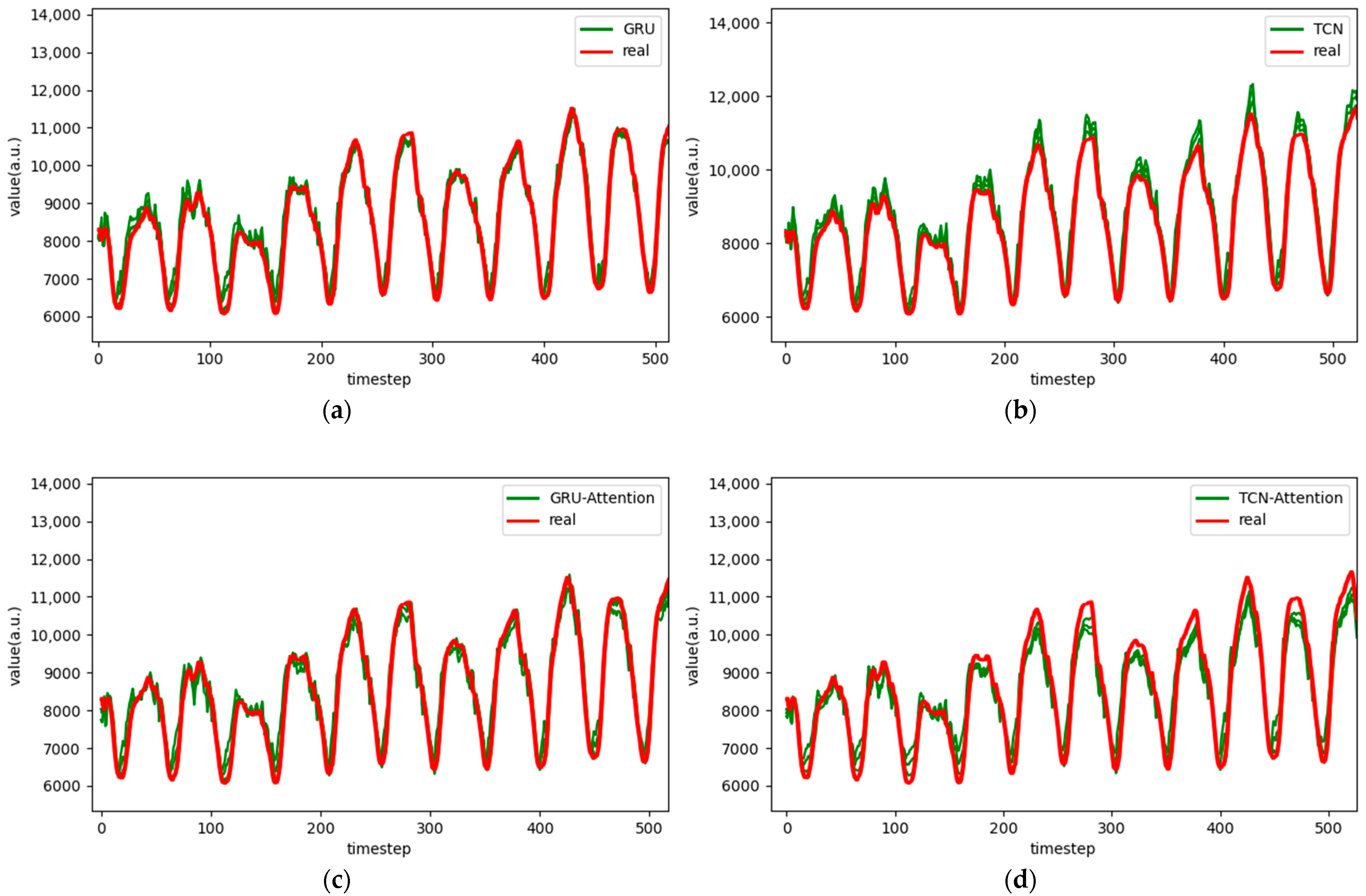
Figure 8.
Comparison chart fitting the 6-step prediction experimental model of the ETTh1 dataset, listed as (a) GRU; (b) TCN; (c) GRU-Attention; (d) TCN-Attention; (e) MrCAN; (f) MSGNet; and (g) Ours.
Figure 8.
Comparison chart fitting the 6-step prediction experimental model of the ETTh1 dataset, listed as (a) GRU; (b) TCN; (c) GRU-Attention; (d) TCN-Attention; (e) MrCAN; (f) MSGNet; and (g) Ours.
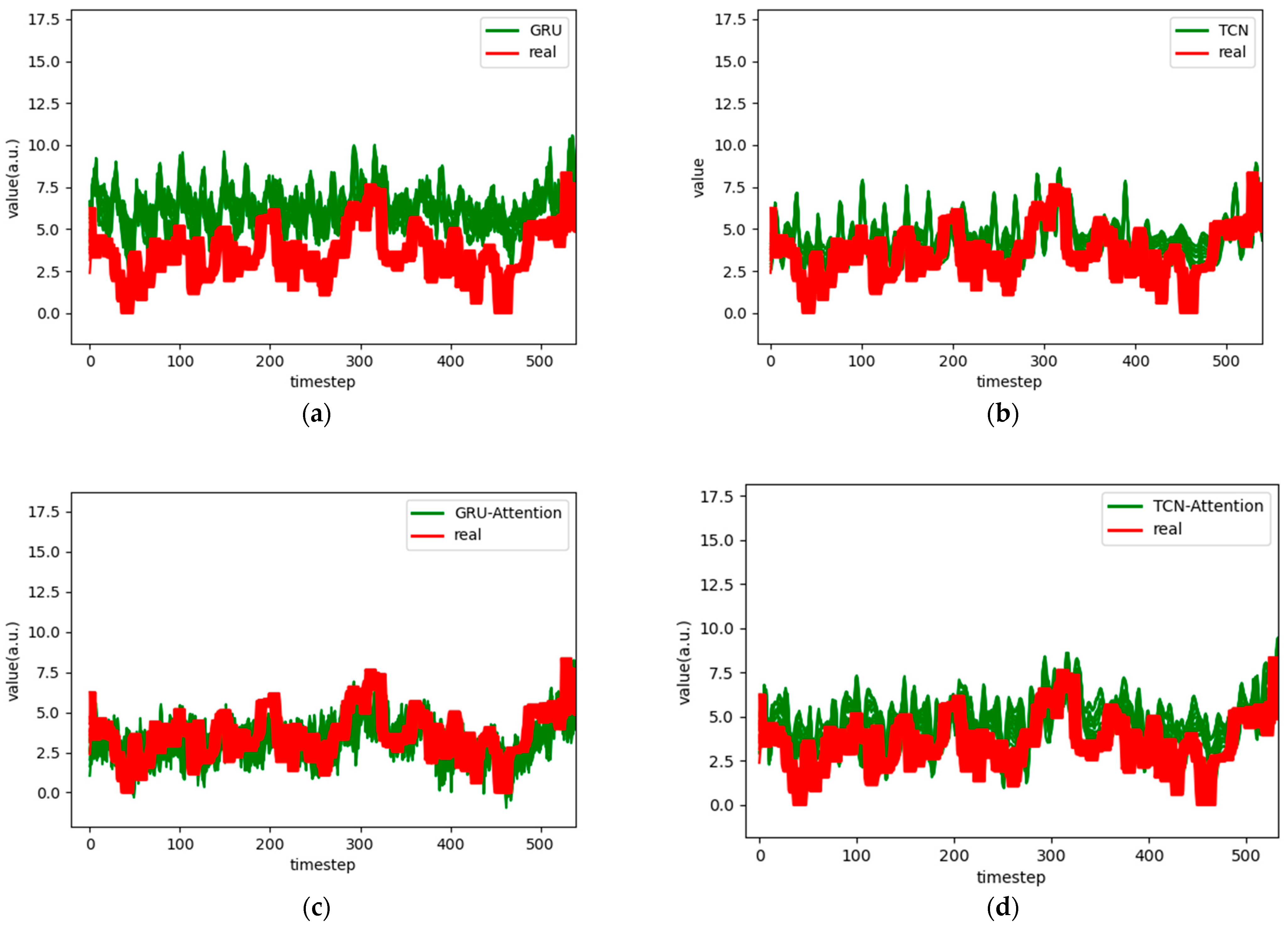
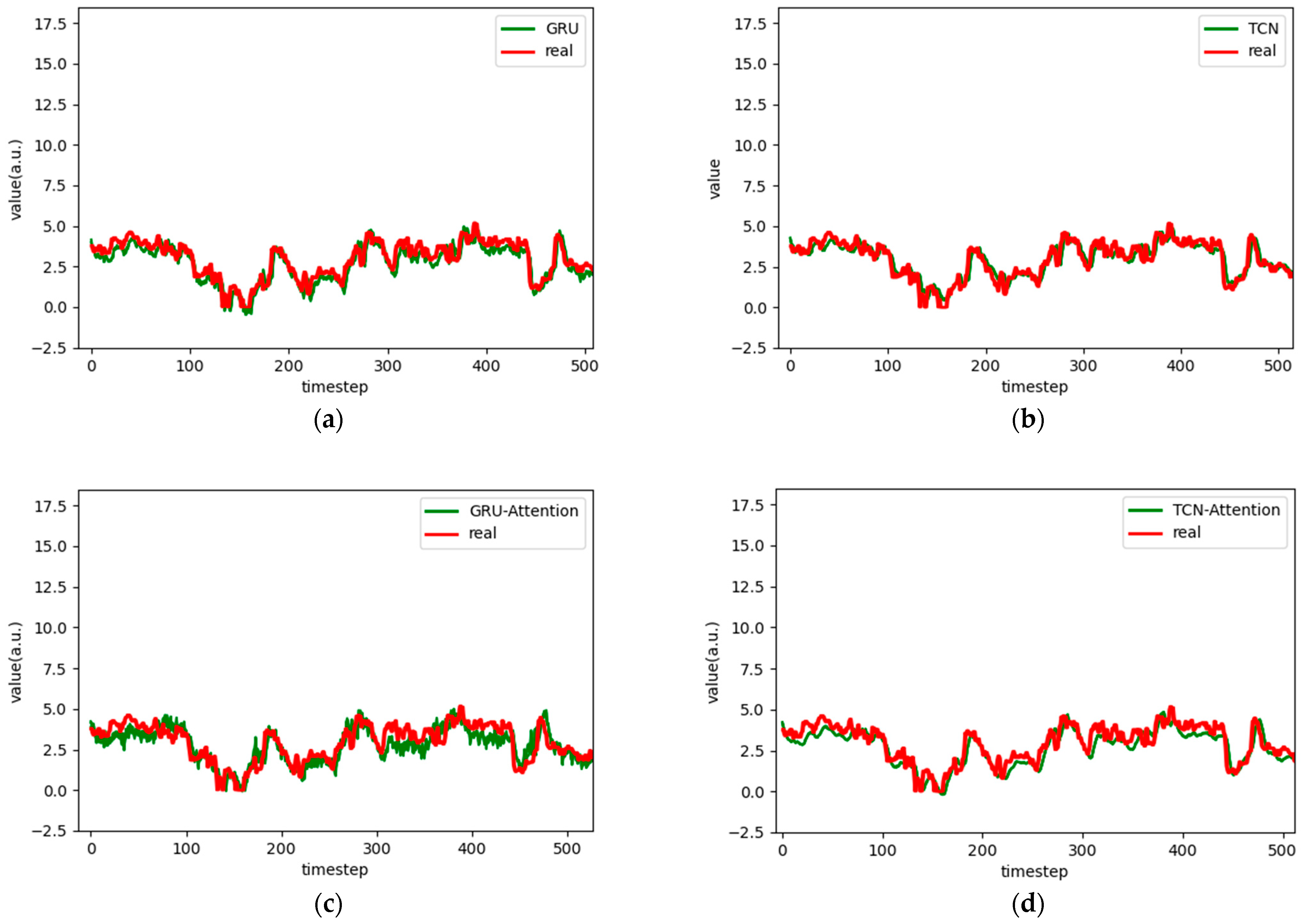
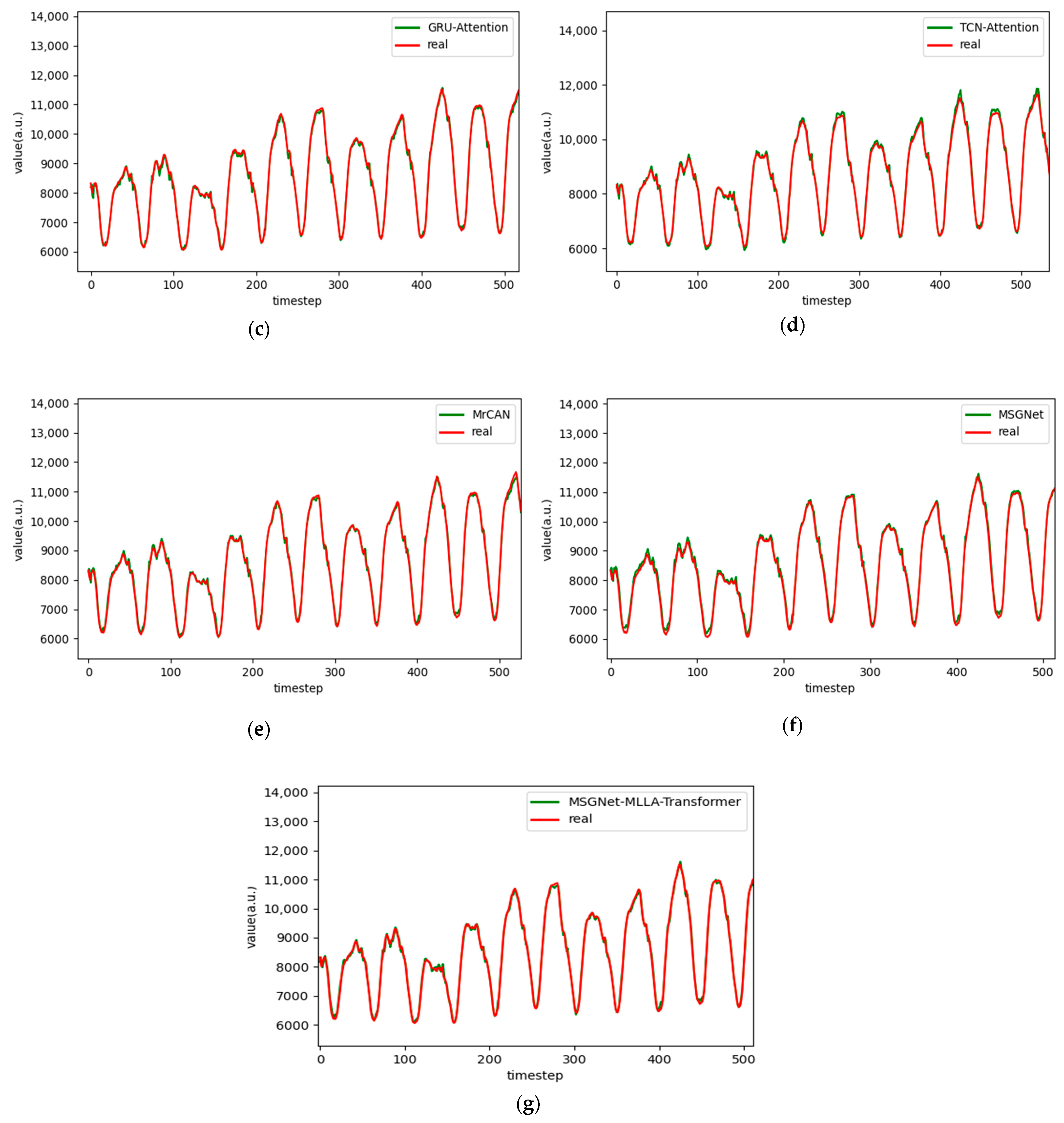
Figure 9.
Comparison chart fitting the 12-step prediction experimental model of the ETTh1 dataset, listed as (a) GRU; (b) TCN; (c) GRU-Attention; (d) TCN-Attention; (e) MrCAN; (f) MSGNet; and (g) Ours.
Figure 9.
Comparison chart fitting the 12-step prediction experimental model of the ETTh1 dataset, listed as (a) GRU; (b) TCN; (c) GRU-Attention; (d) TCN-Attention; (e) MrCAN; (f) MSGNet; and (g) Ours.
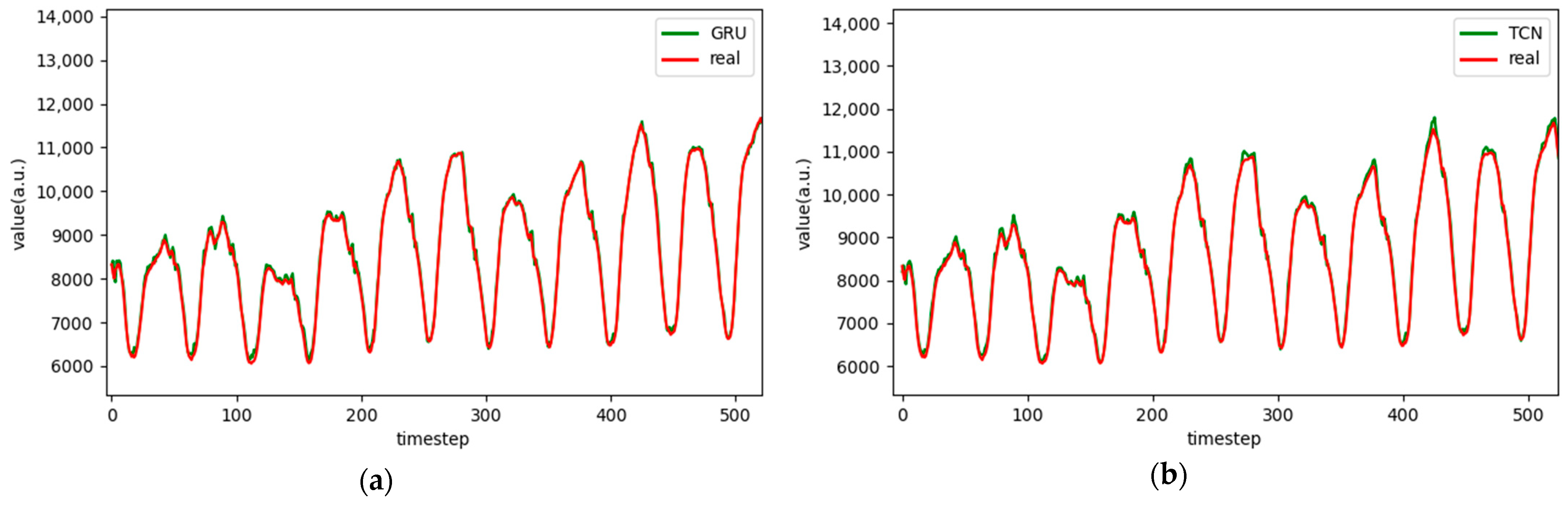
Figure 10.
Comparison chart fitting the 1-step prediction experimental model of the ETTm1 dataset, listed as (a) GRU; (b) TCN; (c) GRU-Attention; (d) TCN-Attention; (e) MrCAN; (f) MSGNet; and (g) Ours.
Figure 10.
Comparison chart fitting the 1-step prediction experimental model of the ETTm1 dataset, listed as (a) GRU; (b) TCN; (c) GRU-Attention; (d) TCN-Attention; (e) MrCAN; (f) MSGNet; and (g) Ours.
Figure 11.
Comparison chart fitting the 3-step prediction experimental model of the ETTm1 dataset, listed as (a) GRU; (b) TCN; (c) GRU-Attention; (d) TCN-Attention; (e) MrCAN; (f) MSGNet; and (g) Ours.
Figure 11.
Comparison chart fitting the 3-step prediction experimental model of the ETTm1 dataset, listed as (a) GRU; (b) TCN; (c) GRU-Attention; (d) TCN-Attention; (e) MrCAN; (f) MSGNet; and (g) Ours.
Figure 12.
Comparison chart fitting the 6-step prediction experimental model of the ETTm1 dataset, listed as (a) GRU; (b) TCN; (c) GRU-Attention; (d) TCN-Attention; (e) MrCAN; (f) MSGNet; and (g) Ours.
Figure 12.
Comparison chart fitting the 6-step prediction experimental model of the ETTm1 dataset, listed as (a) GRU; (b) TCN; (c) GRU-Attention; (d) TCN-Attention; (e) MrCAN; (f) MSGNet; and (g) Ours.
Figure 13.
Comparison chart fitting the 12-step prediction experimental model of the ETTm1 dataset, listed as (a) GRU; (b) TCN; (c) GRU-Attention; (d) TCN-Attention; (e) MrCAN; (f) MSGNet; and (g) Ours.
Figure 13.
Comparison chart fitting the 12-step prediction experimental model of the ETTm1 dataset, listed as (a) GRU; (b) TCN; (c) GRU-Attention; (d) TCN-Attention; (e) MrCAN; (f) MSGNet; and (g) Ours.
Figure 14.
Comparison chart fitting the 1-step prediction experimental model of the Australian electricity load dataset, listed as (a) GRU; (b) TCN; (c) GRU-Attention; (d) TCN-Attention; (e) MrCAN; (f) MSGNet; and (g) Ours.
Figure 14.
Comparison chart fitting the 1-step prediction experimental model of the Australian electricity load dataset, listed as (a) GRU; (b) TCN; (c) GRU-Attention; (d) TCN-Attention; (e) MrCAN; (f) MSGNet; and (g) Ours.
Figure 15.
Comparison chart fitting the 3-step prediction experimental model of the Australian electricity load dataset, listed as (a) GRU; (b) TCN; (c) GRU-Attention; (d) TCN-Attention; (e) MrCAN; (f) MSGNet; and (g) Ours.
Figure 15.
Comparison chart fitting the 3-step prediction experimental model of the Australian electricity load dataset, listed as (a) GRU; (b) TCN; (c) GRU-Attention; (d) TCN-Attention; (e) MrCAN; (f) MSGNet; and (g) Ours.
Figure 16.
Comparison chart fitting the 6-step prediction experimental model of the Australian electricity load dataset, listed as (a) GRU; (b) TCN; (c) GRU-Attention; (d) TCN-Attention; (e) MrCAN; (f) MSGNet; and (g) Ours.
Figure 16.
Comparison chart fitting the 6-step prediction experimental model of the Australian electricity load dataset, listed as (a) GRU; (b) TCN; (c) GRU-Attention; (d) TCN-Attention; (e) MrCAN; (f) MSGNet; and (g) Ours.
Figure 17.
Comparison chart fitting the 12-step prediction experimental model of the Australian electricity load dataset, listed as (a) GRU; (b) TCN; (c) GRU-Attention; (d) TCN-Attention; (e) MrCAN; (f) MSGNet; and (g) Ours.
Figure 17.
Comparison chart fitting the 12-step prediction experimental model of the Australian electricity load dataset, listed as (a) GRU; (b) TCN; (c) GRU-Attention; (d) TCN-Attention; (e) MrCAN; (f) MSGNet; and (g) Ours.
Figure 18.
Graphs showing the results of the ablation experiment indicators for the three datasets, listed as (a) ETTh1; (b) ETTm1; and (c) Australian electricity load.
Figure 18.
Graphs showing the results of the ablation experiment indicators for the three datasets, listed as (a) ETTh1; (b) ETTm1; and (c) Australian electricity load.
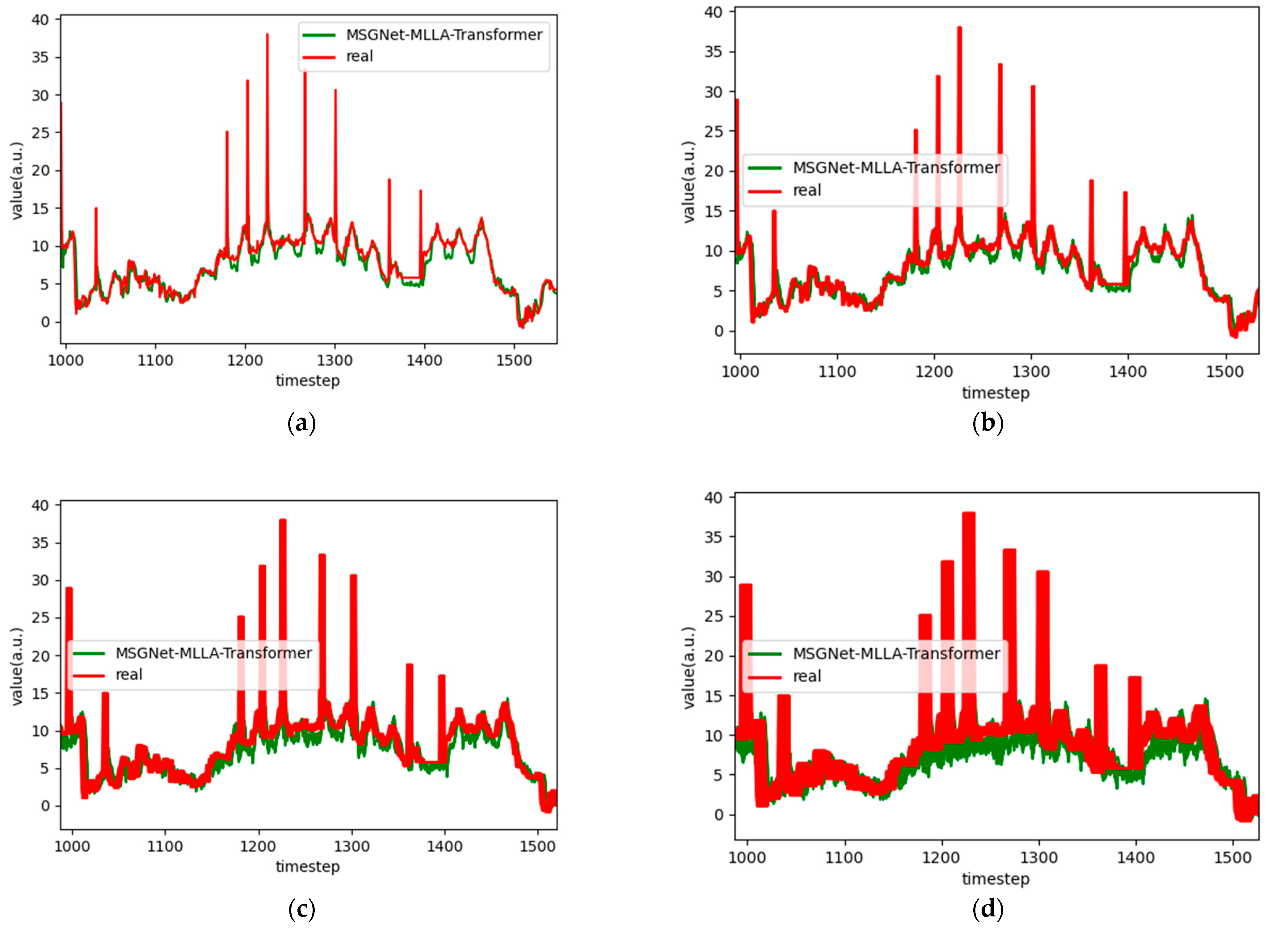
Figure 19.
Graphs of robust analysis results for the ETTh1 dataset, listed as (a) 1-step, (b) 3-step, (c) 6-step, and (d) 12-step.
Figure 19.
Graphs of robust analysis results for the ETTh1 dataset, listed as (a) 1-step, (b) 3-step, (c) 6-step, and (d) 12-step.
Table 1.
Dataset description.
Table 1.
Dataset description.
| Dataset | Prediction Target | Dataset Division (Training Set:Validation Set:Test Set) |
|---|
| ETTh1 | OT | 12,194:1742:3484 |
| ETTm1 | OT | 48,776:6968:13,936 |
| Australian Electricity Load | Electricity Load | 61,354:8765:17,529 |
Table 2.
Model parameter settings.
Table 2.
Model parameter settings.
| Parameters | Values |
|---|
| Learning rate | 0.001 |
| Batch size | 128 |
| Optimizer | Adam [44] |
| Epochs | 200 |
| Dropout | 0.2 |
Table 3.
RMSE, MAE, and evaluation metrics of the ETTh1 dataset.
Table 3.
RMSE, MAE, and evaluation metrics of the ETTh1 dataset.
| Metrics | Method | Predicted Length |
|---|
| 1 | 3 | 6 | 12 |
|---|
| RMSE | ARIMA | 1.900 | 2.418 | 2.732 | 3.348 |
| GRU | 0.942 | 1.107 | 1.266 | 1.702 |
| TCN | 0.806 | 1.206 | 1.511 | 1.968 |
| GRU-Attention | 0.852 | 0.915 | 1.239 | 1.671 |
| TCN-Attention | 0.730 | 1.015 | 1.313 | 1.736 |
| MrCAN | 0.705 | 1.002 | 1.283 | 1.688 |
| MSGNet | 0.741 | 0.931 | 1.210 | 1.662 |
| Ours | 0.664 | 0.904 | 1.197 | 1.656 |
| MAE | ARIMA | 1.691 | 2.112 | 2.493 | 3.016 |
| GRU | 0.772 | 0.745 | 0.940 | 1.311 |
| TCN | 0.601 | 0.946 | 1.143 | 1.542 |
| GRU-Attention | 0.668 | 0.664 | 0.913 | 1.272 |
| TCN-Attention | 0.517 | 0.758 | 1.031 | 1.383 |
| MrCAN | 0.510 | 0.746 | 0.974 | 1.312 |
| MSGNet | 0.559 | 0.677 | 0.887 | 1.263 |
| Ours | 0.481 | 0.642 | 0.863 | 1.262 |
| ARIMA | 0.731 | 0.683 | 0.554 | 0.328 |
| GRU | 0.925 | 0.913 | 0.865 | 0.756 |
| TCN | 0.945 | 0.877 | 0.807 | 0.675 |
| GRU-Attention | 0.939 | 0.929 | 0.871 | 0.767 |
| TCN-Attention | 0.951 | 0.913 | 0.855 | 0.746 |
| MrCAN | 0.958 | 0.915 | 0.861 | 0.760 |
| MSGNet | 0.953 | 0.927 | 0.876 | 0.768 |
| Ours | 0.963 | 0.931 | 0.880 | 0.769 |
Table 4.
RMSE, MAE, R2 evaluation metrics of the ETTm1 dataset.
Table 4.
RMSE, MAE, R2 evaluation metrics of the ETTm1 dataset.
| Metrics | Method | Predicted Length |
|---|
| 1 | 3 | 6 | 12 |
|---|
| RMSE | ARIMA | 1.432 | 2.857 | 3.586 | 4.338 |
| GRU | 0.460 | 0.640 | 0.751 | 0.951 |
| TCN | 0.385 | 0.690 | 0.879 | 0.999 |
| GRU-Attention | 0.510 | 0.658 | 0.894 | 0.963 |
| TCN-Attention | 0.678 | 0.857 | 0.943 | 0.956 |
| MrCAN | 0.378 | 0.606 | 0.728 | 0.913 |
| MSGNet | 0.365 | 0.514 | 0.735 | 0.855 |
| Ours | 0.346 | 0.470 | 0.613 | 0.855 |
| MAE | ARIMA | 1.217 | 2.625 | 3.398 | 4.164 |
| GRU | 0.370 | 0.518 | 0.577 | 0.719 |
| TCN | 0.292 | 0.551 | 0.642 | 0.731 |
| GRU-Attention | 0.378 | 0.500 | 0.670 | 0.710 |
| TCN-Attention | 0.580 | 0.640 | 0.799 | 0.704 |
| MrCAN | 0.283 | 0.471 | 0.560 | 0.676 |
| MSGNet | 0.273 | 0.352 | 0.531 | 0.611 |
| Ours | 0.252 | 0.320 | 0.415 | 0.603 |
| ARIMA | 0.736 | 0.682 | 0.545 | 0.331 |
| GRU | 0.966 | 0.955 | 0.942 | 0.913 |
| TCN | 0.970 | 0.949 | 0.935 | 0.906 |
| GRU-Attention | 0.958 | 0.953 | 0.932 | 0.908 |
| TCN-Attention | 0.951 | 0.938 | 0.925 | 0.923 |
| MrCAN | 0.971 | 0.959 | 0.945 | 0.920 |
| MSGNet | 0.972 | 0.967 | 0.942 | 0.928 |
| Ours | 0.979 | 0.971 | 0.958 | 0.928 |
Table 5.
RMSE, MAE, evaluation metrics of the Australian electricity load dataset.
Table 5.
RMSE, MAE, evaluation metrics of the Australian electricity load dataset.
| Metrics | Method | Predicted Length |
|---|
| 1 | 3 | 6 | 12 |
|---|
| RMSE | ARIMA | 1114.640 | 1497.295 | 2427.290 | 2969.202 |
| GRU | 132.349 | 388.518 | 753.815 | 1157.247 |
| TCN | 319.052 | 477.217 | 856.929 | 1277.548 |
| GRU-Attention | 126.481 | 335.018 | 583.403 | 980.216 |
| TCN-Attention | 180.761 | 381.154 | 591.088 | 1045.967 |
| MrCAN | 132.296 | 307.270 | 576.016 | 884.175 |
| MSGNet | 132.257 | 310.001 | 564.320 | 828.189 |
| Ours | 109.301 | 292.855 | 518.900 | 783.182 |
| MAE | ARIMA | 1099.937 | 1276.531 | 2101.269 | 2735.886 |
| GRU | 99.840 | 279.779 | 552.986 | 878.398 |
| TCN | 235.910 | 390.566 | 708.918 | 1067.904 |
| GRU-Attention | 94.676 | 242.491 | 417.174 | 730.904 |
| TCN-Attention | 134.382 | 275.569 | 425.921 | 819.309 |
| MrCAN | 100.884 | 218.761 | 414.341 | 650.945 |
| MSGNet | 99.612 | 224.166 | 410.227 | 658.960 |
| Ours | 81.107 | 216.314 | 380.461 | 574.777 |
| ARIMA | 0.426 | 0.391 | 0.283 | −0.494 |
| GRU | 0.980 | 0.920 | 0.699 | 0.290 |
| TCN | 0.936 | 0.879 | 0.611 | 0.135 |
| GRU-Attention | 0.982 | 0.941 | 0.816 | 0.491 |
| TCN-Attention | 0.972 | 0.923 | 0.819 | 0.420 |
| MrCAN | 0.980 | 0.950 | 0.824 | 0.585 |
| MSGNet | 0.980 | 0.949 | 0.831 | 0.636 |
| Ours | 0.984 | 0.954 | 0.857 | 0.675 |
Table 6.
Robustness analysis metrics of the ETTh1 dataset.
Table 6.
Robustness analysis metrics of the ETTh1 dataset.
| Dataset | Metrics | Predicted Length |
|---|
| 1 | 3 | 6 | 12 |
|---|
| ETTh1 | RMSE | 1.800 | 1.963 | 2.301 | 2.567 |
| MAE | 0.872 | 0.909 | 1.327 | 1.589 |
| 0.932 | 0.924 | 0.868 | 0.755 |
| ETTh2 | | 0.533 | 0.617 | 0.728 | 0.981 |
| 0.383 | 0.472 | 0.590 | 0.803 |
| 0.966 | 0.959 | 0.954 | 0.931 |
| Australian Electricity Load | | 216.247 | 401.082 | 665.439 | 892.131 |
| 193.460 | 314.960 | 582.718 | 719.004 |
| 0.973 | 0.948 | 0.836 | 0.682 |
Table 7.
Computational cost of MSGNet-MLLA-Transformer on the Australian electricity load dataset.
Table 7.
Computational cost of MSGNet-MLLA-Transformer on the Australian electricity load dataset.
| Method | Predicted Length |
|---|
| Training Time | Inference Time | RMSE |
|---|
| Ours | 0.178 s | 0.0457 s | 783.182 |
| MSGNet | 0.266 s | 0.084 s | 828.189 |
| MrCAN | 0.087 s | 0.025 s | 884.175 |


