Forecasting Day-Ahead Electricity Demand in Australia Using a CNN-LSTM Model with an Attention Mechanism

Abstract

Accurate energy demand forecasting is vital for optimizing resource allocation and energy efficiency. Despite advancements in various prediction models, existing approaches often struggle to capture the complex, nonlinear relationships between temperature variations and electricity consumption. To address this issue, this paper introduces a novel hybrid deep learning model that integrates Convolutional Neural Networks (CNNs) and Long Short-Term Memory (LSTM) networks with an attention mechanism designed to forecast day-ahead electricity demand in Australia. This research aims to enhance the accuracy of electricity demand predictions by effectively modeling the impact of heating degree days (HDDs) and cooling degree days (CDDs) on energy usage. The HDDs and CDDs capture extreme weather conditions. They are critical for understanding spikes in energy consumption for heating and cooling needs. The proposed model leverages the strengths of CNNs in extracting spatial features in HDDs and CDDs, LSTMs in capturing temporal dependencies, and the attention mechanism in focusing on the most relevant aspects of the data. This study compares the CNN-LSTM-Attention model with traditional methods, including Deep Neural Networks, and demonstrates superior performance. The results show a significant reduction in both Mean Absolute Error and Mean Absolute Percentage Error, confirming the model’s effectiveness. The primary contribution of this paper lies in the novel integration of CDD and HDD data within the CNN-LSTM framework, which has not been extensively explored in prior studies. This approach offers a robust solution for energy management, particularly in climates with significant temperature fluctuations.

1. Introduction

The accurate prediction of future energy demand enables better planning and operation for electricity providers, allowing them to prepare adequately and avoid issues of overproduction or underproduction. This not only reduces costs but also increases the efficiency of the energy industry. Electricity demand can be predicted using two primary methods: physical model-based approaches and data-driven techniques. Physical models are easy to understand and implement. However, the high computational cost required can make real-time forecasting or large-scale simulations impractical in some cases [1]. Furthermore, aggregating multiple physical models, each with inherent uncertainties, can decrease the overall accuracy of the forecast, especially for large-scale prediction problems [2].

Data-driven techniques are further categorized into statistical and machine learning methods. Statistical methods often utilize a regression analysis or time series prediction. Regression analysis involves creating mathematical models that define the relationships between independent and dependent variables to forecast electricity demand. For example, an enhanced multivariable linear regression model has been employed to predict daily average cooling loads in office buildings [3]. Time series analysis, another statistical method, was used to handle dynamic data for prediction purposes. Although these statistical methods are straightforward, they can struggle with complex interactions between input variables, leading to lower calculation efficiency and accuracy [4].

Machine learning and data mining techniques have attracted much attention worldwide for both short-term and long-term electricity demand forecasting. Many deep learning models have been employed to predict electricity demand or load, such as Convolutional Neural Networks (CNNs), Deep Neural Networks (DNNs), and Long Short-Term Memory (LSTM). These models can independently learn and predict electricity demand by scrutinizing energy usage patterns, effectively addressing the nonlinear problem [5].

Reference [6] presented a short-term load prediction model based on a DNN and the stacked ensemble method. In the study of [7], the authors applied a multiple regression model alongside three CNNs to forecast Florida’s future electricity usage. The multiple regression model results indicated that the variable month, cooling degree days (CDDs), heating degree days (HDDs), and gross domestic product (GDP) were significant predictors of future electricity demand. Reference [8] developed two regression models—ordinal and multiple linear regression—to predict electricity demand in Greece, utilizing seventeen years of historical data that included economic, weather, and energy efficiency variables. This study concluded that the GDP had the most significant influence on electricity demand, with HDDs and CDDs also playing important roles. The ordinal model achieved a Mean Absolute Percentage Error (MAPE) of 0.74%. Another study examined the impact of climate variables on electricity demand in Sydney, Australia, using a backward selection multiple regression model. Ten years of historical data were analyzed, and the model produced an R-square value of 0.816, identifying the CDD, wind speed, evaporation, and humidity as significant variables [9]. Reference [10] also applied multiple linear regression to forecast hourly and monthly electricity demand in a region of Australia, identifying the CDD, HDD, humidity, and the number of rainy days as key predictors.

Many data-driven methods have been used for long-term load forecasting for strategic power system planning. Conventionally, long-term load forecasting has relied on Artificial Neural Networks (ANNs) or regression-based methods, utilizing extensive historical data on electricity load, weather, economic factors, and population. However, these classical approaches have limitations, such as insensitivity to changing trends over long periods and difficulty in managing a large number of variables and complex relationships. To address these challenges, a novel sequence-to-sequence hybrid model was introduced in [11], which combines the CNN with LSTM networks to forecast monthly peak loads over a three-year horizon. By focusing on the monthly peak load, the model avoided unnecessary complications while still providing all the essential information needed for effective long-term strategic planning. The accuracy of the proposed method was validated using load data from New South Wales (NSW), Australia, with numerical results demonstrating superior prediction accuracy compared to existing long-term load forecasting models.

To further improve the prediction accuracy of electricity demand, some other strategies have been employed recently, such as a combination of various machine learning models and using the latest deep learning models with an attention mechanism. In [12], the authors utilized a CNN-LSTM model with an attention mechanism to forecast electricity demand within a smart grid environment. Their findings indicated that the attention-enhanced model outperformed conventional CNN-LSTM models, achieving a reduced MAPE and Mean Absolute Error (MAE). Reference [13] utilized a CNN-LSTM model with an attention mechanism to predict day-ahead electricity demand in a renewable energy-heavy grid. The model combined historical demand data with weather factors such as temperature, wind speed, and solar radiation. Their results demonstrated that this approach can significantly improve the forecasting performance compared to conventional models, making it particularly useful for managing the variability and uncertainty inherent in renewable energy sources. In the study of [14], the author developed an enhanced sequence-to-sequence GRU model capable of capturing dynamic temporal dependency patterns in the data. This model used calendar, weather, and historical load data to achieve its predictions. The author of [15] applied the Temporal Fusion Transformer (TFT) model for electricity demand forecasting. This model leverages self-attention mechanisms to capture the relationships between various elements in a sequence.

Despite the advancements in electricity demand forecasting, existing models still face challenges in capturing the complex and dynamic nature of electricity consumption, especially in the context of varying climatic conditions. Most conventional models, including those utilizing machine learning and regression-based approaches, often struggle to adequately account for the nonlinear relationships between multiple influencing factors such as temperature fluctuations, economic activity, and energy usage patterns over time. Moreover, while some studies have incorporated weather variables like the HDD and CDD, there is still a lack of integration of advanced techniques that can enhance prediction accuracy by focusing on the most relevant data points. This research addresses these issues by introducing a hybrid CNN-LSTM model enhanced with an attention mechanism. The proposed model distinctly utilizes HDD and CDD data to effectively capture the significant impact of temperature fluctuations on energy demand. It improves the precision of day-ahead electricity demand forecasting. It is a reliable energy management tool, particularly in regions such as NSW, Australia, where climate variability greatly influences energy consumption patterns.

The rest of this paper is organized as follows: Section 2 presents the proposed prediction model. Section 3 demonstrates the prediction results of various models, including the proposed model, and discusses the results. Finally, Section 4 concludes this paper.

2. The Proposed Prediction Method

The proposed prediction method was divided into four main steps: data collection, pre-processing of the data, constructing benchmark DL models, and building the CNN-LSTM-Attention model.

• Step 1: Data Collection

The dataset used in this study was aggregated by combining the energy data from AEMO’s dataset with the weather data from the Sydney Bureau of Meteorology. This dataset contains 8640 records per year, which includes hourly electricity demand (MW) and hourly weather parameters. The weather data that were utilized to build the benchmark and the proposed electricity demand prediction models include the temperature (°C), humidity (%), wind speed (km/h), CDD (Degree-days), and HDD (Degree-days). The dataset range utilized for the forecasting model in this study spans from January 2020 to December 2020. In addition, the models were evaluated based on the data from the years 2022 and 2023.

CDD and HDD are critical indices that quantify the impact of temperature on energy consumption. The degree day is a numerical index initially developed by engineers specializing in heating, ventilation, and air conditioning [16]. The HDD index assumes that people will start using their furnaces when the average daily temperature falls below a specific threshold. In NSW, the heating critical temperature (CT) was set to 17 °C by the Australian National Electricity Market (NEM) [17]. The CDD index evaluates the energy demands necessary to cool buildings and residences. When the average daily temperature exceeds a specific threshold, individuals will start using measures such as air conditioning to cool their surroundings. In NSW, the cooling critical temperature was set to 19.5 °C by NEM [17]. By incorporating CDD and HDD into our hybrid CNN-LSTM model, we can accurately model the temperature sensitivity of energy demand. This approach is particularly valuable for forecasting in climates like NSW, where seasonal temperature changes lead to substantial fluctuations in energy usage.

• Step 2: Data Pre-Processing

The electricity demand dataset comprises 8760 hourly entries spanning 1 January 2020, to 31 December 2020, with features including DEMAND, temperature, wind speed, humidity, heat index, CDD, and HDD. This dataset was used to train a CNN-LSTM-Attention model for electricity demand forecasting. Given the model’s reliance on sequential input features and its sensitivity to temporal dependencies and feature scales, several preprocessing steps were applied to optimize the data for analysis.

An initial assessment identified a minor proportion of missing values within the dataset, primarily in the wind speed and humidity features, accounting for approximately 1.5% of the total entries. To address this, we imputed missing values using the mean value of the respective feature, calculated across the entire dataset.

To ensure consistent input scales for the CNN and LSTM layers of the CNN-LSTM-Attention model, we standardized the numerical features using the standardization formula:

$$X_{stand}={\displaystyle \frac{x-\mu }{\sigma }}$$

(1)

where X_stand is the standardized variable, $x$ is the actual value, µ is the mean, and σ is the standard deviation.

Standardization was implemented using the StandardScaler from the scikit-learn library, with parameters fitted on the training set and applied to both training and test sets to prevent data leakage. After standardization, all features had a mean of 0 and a standard deviation of 1, which facilitated faster convergence during training and improved the model’s ability to learn temporal patterns. The target variable (DEMAND) was similarly standardized to align with the model’s input–output scale, with an inverse transformation applied to obtain predictions in the original MW scale. This preprocessing step notably improved prediction accuracy, as evidenced by a reduction in the Mean Absolute Percentage Error (MAPE) during model training.

To ensure a robust evaluation and minimize the risk of overfitting in our electricity demand forecasting model, we implemented a 5-fold cross-validation strategy using TimeSeriesSplit from the scikit-learn library [18]. This time-based cross-validation method preserves the chronological order of the data, ensuring that training sets consistently preceded validation sets temporally.

• Step 3: Benchmark Deep Learning Models:

The proposed energy prediction model was compared with many benchmark deep learning models such as DNNs and CNNs. Integrating various deep learning algorithms significantly improved the accuracy of energy demand prediction. The configuration details of the benchmark deep learning models are presented in

Table 1. Configuration of the benchmark models.

Hyper Parameter	Setting
Layers—DNN—(Fully Connected)	Dense—64
Layers—CNN	Conv1D—128 MaxPooling1D—128
Layers—LSTM	64
Batch Size	128
Dropout	0.25
Epochs	500
Activation Function	ReLU
Optimizer	Adam
Loss	MAE, MAPE

.

• Step 4: CNN-LSTM with Attention Mechanism for Prediction:

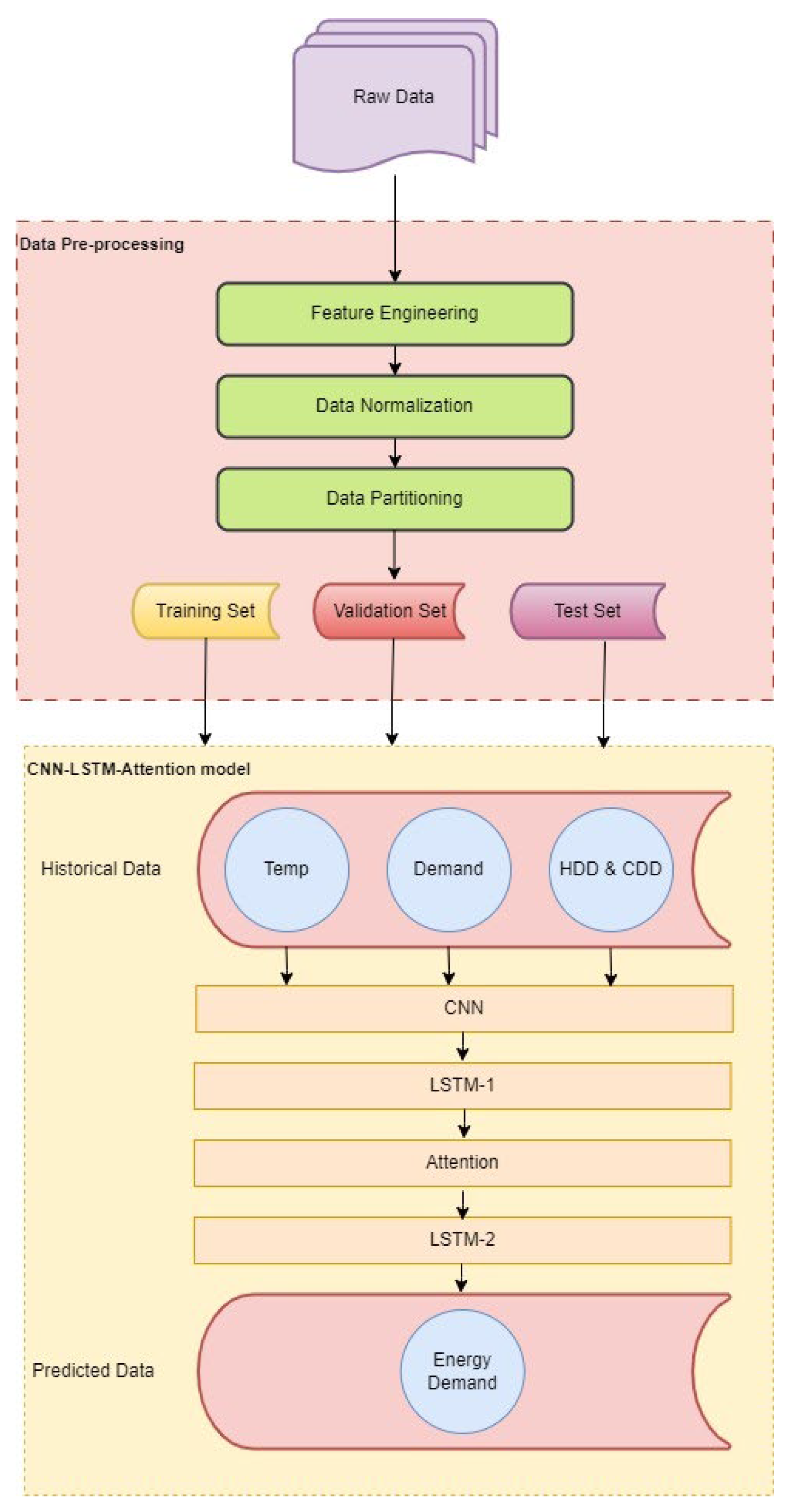
The proposed energy prediction model architecture, which is based on CNN-LSTM with a self-attention model, is used to predict energy demand based on HDDs and CDDs. Figure 1 depicts the structure of the proposed model.

The proposed model integrates CNN and LSTM algorithms with an attention mechanism. The soft attention technique is expressed as follows:

$$O=softmax({\displaystyle \frac{Q{K}^T}{\sqrt{d_k}}})V$$

(2)

where O is the output of the attention mechanism, Q is the query matrix, K is the key matrix, V is the value matrix, and $d_k$ is the dimension of the key vectors.

The CNN algorithm plays a vital role in feature extraction from the input features. The CNN consists of twenty convolution layers with another twenty pooling layers; each layer consists of 128 neurons. To avoid the risk of overfitting, a dropout layer with a 20% rate was incorporated. The outputs of the CNN algorithms were then fed into a two-layer LSTM, each layer comprising 64 neurons, to enable sequence prediction. The output of the first LSTM layer was passed to a self-attention layer, which focuses on specific network features by assigning weights to relevant temporal dependencies. The second LSTM layer, integrated with an attention mechanism and a dropout layer, employed the same number of neurons (64) and dropout rate (20%) as the first LSTM layer. Nonlinearity was introduced via the Rectified Linear Unit (ReLU) activation function across the proposed CNN-LSTM-Attention model. Finally, a dense layer with a ReLU activation function processes the output to generate the model’s predictions.

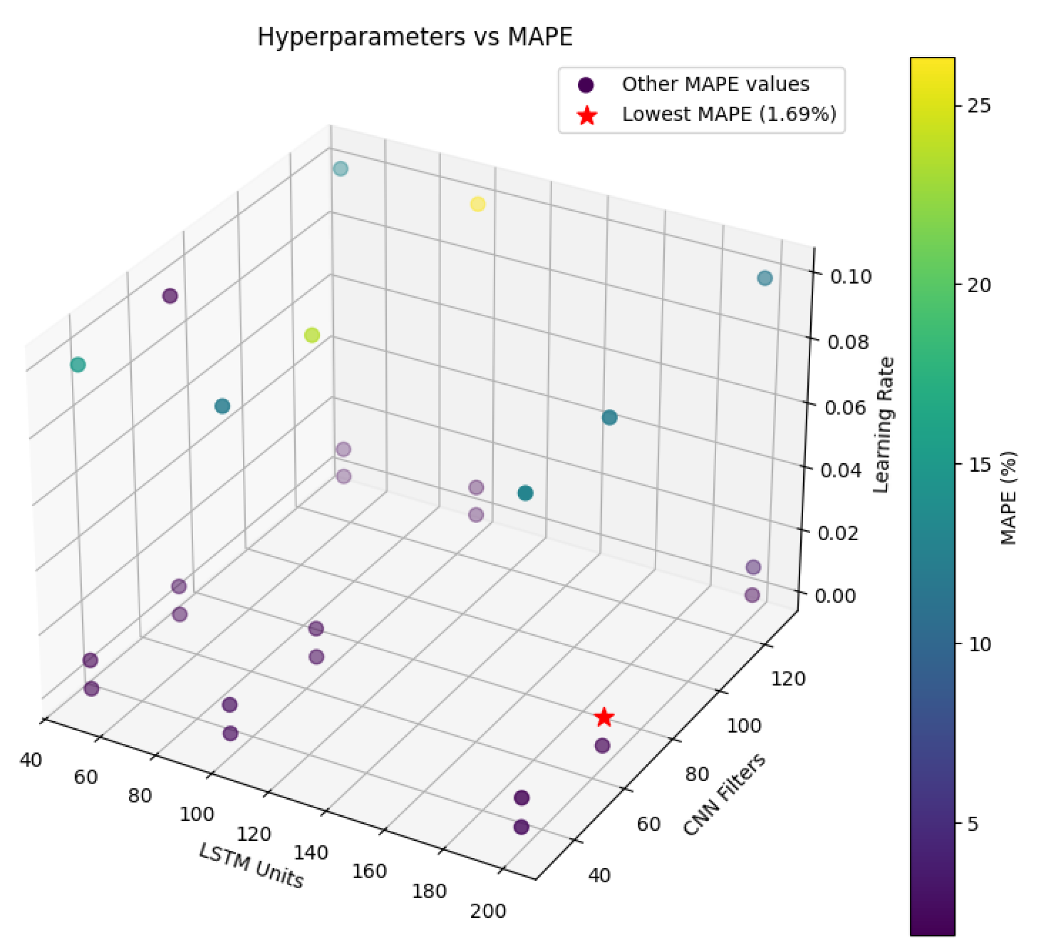
To systematically identify the optimal hyperparameter values and enhance model robustness, grid search was applied during the training phase. A comprehensive experimental evaluation was conducted to analyze the effects of various hyperparameters, including the number of LSTM units, filters, and learning rate, on model performance.

Table 2. Impact of hyperparameter tuning on MAPE.

		MAPE
Filters	LSTM Units	Learning Rate
		0.1	0.01	0.001
32	50	15.24	1.88	1.95
32	100	12.17	2.54	2.40
32	200	12.94	2.10	2.44
64	50	1.96	2.32	1.99
64	100	23.58	2.15	2.21
64	200	12.11	1.69	1.99
128	50	13.24	2.20	2.08
128	100	26.33	1.96	2.00
128	200	11.80	3.44	1.88

presents the impact of different hyperparameter settings, such as the number of filters, LSTM units, and learning rates on MAPE. For instance, the first row shows a configuration with 32 filters and 50 LSTM units, yielding MAPE values of 15.24, 1.88, and 1.95 for learning rates of 0.1, 0.01, and 0.001, respectively.

A visual representation of the hyperparameter analysis is provided in Figure 2, which illustrates the relationship between LSTM units, CNN filters, learning rate, and MAPE across all tested configurations.

In this study, all model structures and layers were constructed using Google TensorFlow 2.16.1 and the Keras library 2.16.1. During the experimental phase, the proposed model and the baseline models were trained and evaluated on Google Colab. The configuration details of the proposed model are presented in

Table 3. Configuration of the proposed model.

Hyper Parameter	Setting
Epochs	500
Batch Size	128
Activation Function	ReLU
FC Layer	64
LSTM Layer	64
Optimizer	Adam
Loss	MAE
Attention Type	Soft

.

3. Results and Discussion

3.1. Prediction Results and Comparisons

The Adam (Adaptive Moment Estimation) optimizer is among the most widely used optimization algorithms for training deep learning models. It combines the advantages of two other extensions of Stochastic Gradient Descent (SGD): AdaGrad and RMSProp. By adjusting the learning rate for each parameter individually, Adam accelerates the convergence of the training process and can enhance the overall performance. Therefore, Adam optimizer has been chosen for all DL models in this study. Two error indicators are used in this study to assess the performance of the proposed model and other models. They are MAE and MAPE and are defined as follows:

$$MAE={\displaystyle \frac{\sum _{i=1}^n|y_i-x_i|}{n}}$$

(3)

$$MAPE={\displaystyle \frac{1}{n}} {\sum }_{i=1}^n\left|{(y}_i-x_i)/x_i\right|\ast 100$$

(4)

where $y_i$ is the predicted value, $x_i$ is the actual value at a given time, and $n$ is the number of samples.

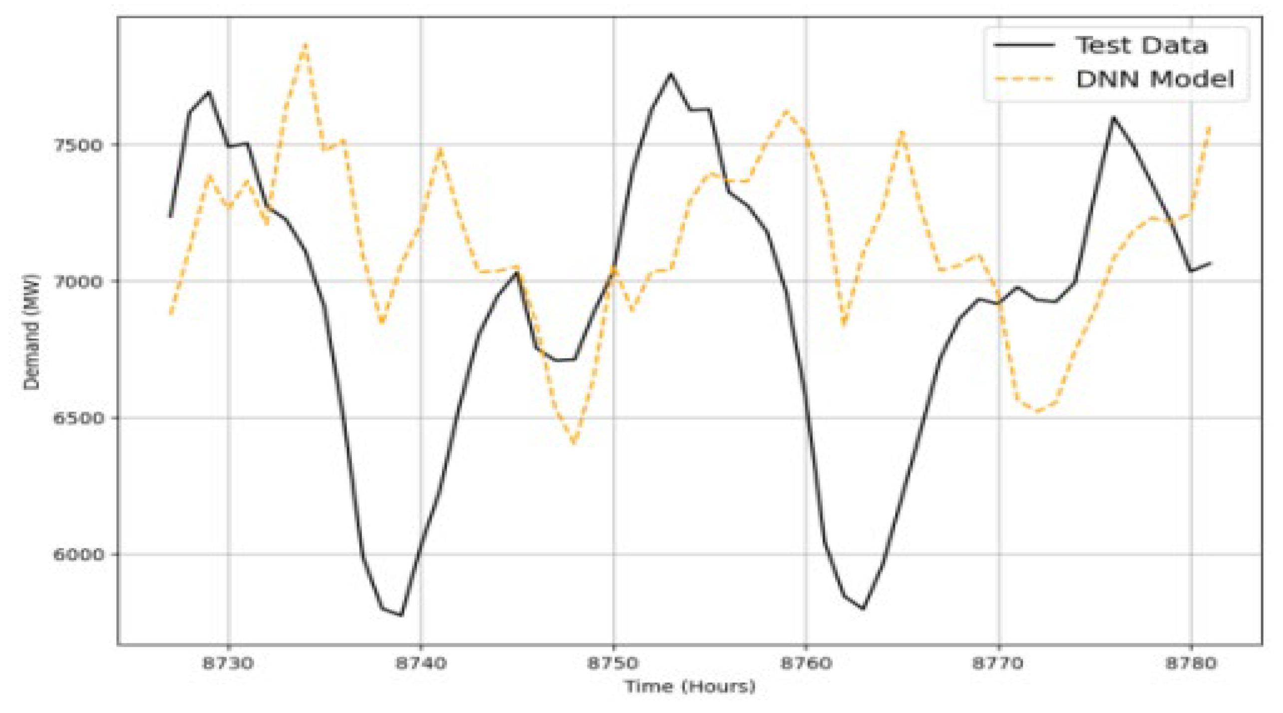
First, as a benchmark to compare all models, Figure 3 shows the forecasting results using the DNN model. As shown, the electricity prediction using the DNN model only is not promising.

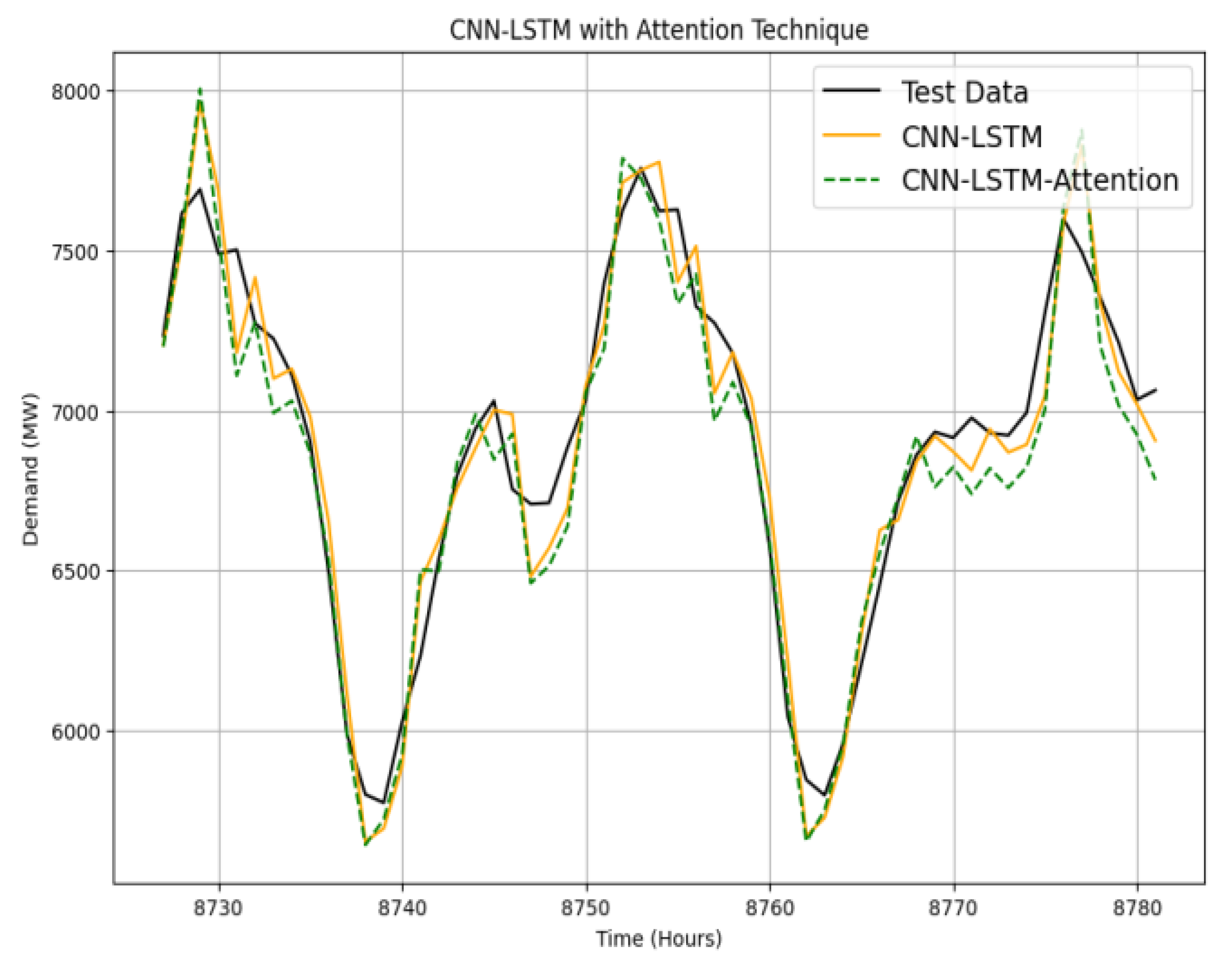
Figure 4 illustrates the prediction results using hybrid CNN and LSTM models with and without an attention mechanism. The HDD and CDD are integrated into the hybrid prediction models. As shown, the integration of CNNs and LSTM networks in the proposed hybrid model has shown significant promise in capturing the complex temporal and spatial dependencies inherent in electricity demand forecasting. CNNs are particularly effective in extracting local patterns and spatial features from the input data, such as the variations in the HDD and CDD, which are critical in understanding the impact of temperature on energy consumption. By passing these extracted features into the LSTM layers, the model can capture long-term dependencies and sequential relationships within the data, which are essential for accurate forecasting over time. This dual approach ensures that both spatial and temporal aspects of the data are effectively utilized, leading to more accurate predictions than models relying solely on one type of neural network.

Table 4. Evaluation metrics for the dataset of year 2020.

Model	MAE	MAE Improvement of the Proposed Model	MAPE	MAPE Improvement of the Proposed Model
CNN	838	85.44%	11.9	85.80%
DNN	807	84.88%	11	84.64%
DNN and CNN	153.3	20.42%	2.1	19.52%
DNN and LSTM	138	11.59%	1.89	10.58%
CNN and LSTM	135	9.63%	1.83	7.65%
CNN and LSTM with Attention	122	--	1.69	--

lists the performance of various models, including the baseline DNN, CNN, LSTM, and the proposed hybrid models, for the 2020 dataset. It offers a detailed comparison of MAE, MAPE, and the percentage improvement of the proposed method compared with other methods.

First, the MAE and MAPE of CNN are 838 and 11.9, respectively; the MAE and MAPE of DNN are 807 and 11, respectively.

Second, to enhance prediction accuracy, three hybrid models with two from CNN, DNN, and LSTM models are trained and compared. The MAE and MAPE of a hybrid model with CNN and DNN are 153.3 and 2.1, respectively; the MAE and MAPE of a hybrid model with DNN and LSTM are 138 and 1.89, respectively; and the MAE and MAPE of a hybrid model with CNN and LSTM are 135 and 1.83, respectively. Integrating the DNN-CNN model improved the prediction accuracy by 81% and 81.7%, compared with the DNN and CNN model, respectively. Integrating the CNN-LSTM model has further improved the prediction accuracy by 83% and 83.9% compared to the DNN and CNN only. These models represent key steps in the development of more advanced hybrid architectures, such as the proposed CNN-LSTM with attention model.

Third, for the proposed model (a hybrid model with the CNN and LSTM and attention mechanism), its MAE and MAPE are 122 and 1.69, respectively. The MAE and MAPE of the proposed model are the smallest ones among these models, highlighting the effectiveness of the proposed approaches. The proposed CNN-LSTM with attention model substantially improves prediction accuracy. For instance, it reduces the MAE by approximately 84.88% compared to the baseline DNN model and 9.63% compared to the standard CNN-LSTM model. These improvements underscore the effectiveness of integrating the attention mechanism into the CNN-LSTM architecture, particularly in capturing the most relevant features for accurate electricity demand forecasting.

In summary, in the evaluation of the CNN-LSTM model, the results indicate that it outperforms traditional models, such as the DNN, in terms of the MAE and MAPE. This demonstrates the effectiveness of combining CNN and LSTM architectures in a hybrid model for electricity demand forecasting. The reduction in the MAE and MAPE highlights the model’s ability to more accurately predict energy demand, which is crucial for efficient resource allocation and management. However, while the CNN-LSTM hybrid model improves prediction accuracy, it has limitations. One of the challenges observed is that the model’s performance can be sensitive to the choice of hyperparameters, such as the number of filters in the CNN and the number of neurons in the LSTM layers. This sensitivity requires careful tuning and extensive experimentation to achieve optimal results, which can be computationally intensive. Additionally, the model may struggle with capturing very long-term dependencies beyond a certain threshold, like LSTMs, despite their design to handle long sequences, and can still face difficulties when the sequence length becomes exceedingly large. This limitation suggests that further enhancements, such as incorporating attention mechanisms, could improve the model’s ability to focus on the most relevant time steps in the sequence. Therefore, integrating the attention approach in the CNN-LSTM model has achieved higher electricity prediction accuracy than the hybrid CNN-LSTM model.

Table 5. Evaluation metrics for the dataset of years 2022 and 2023.

		2022		2023
No.	Model	MAE	MAPE	MAE	MAPE
1	CNN	1096	17.9	1102	18
2	DNN	816	11.3	1010	16
3	DNN-LSTM	216	3.11	217	3.13
4	CNN and LSTM—Attention	171	2.2	194	2.4

presents the results of applying both the base models and the proposed model to the data from the years 2022 and 2023. As can be seen, the proposed model’s MAE and MAPE are the smallest among these models. Therefore, the advantages of the proposed models can be verified.

3.2. Learning Curves and Model Features

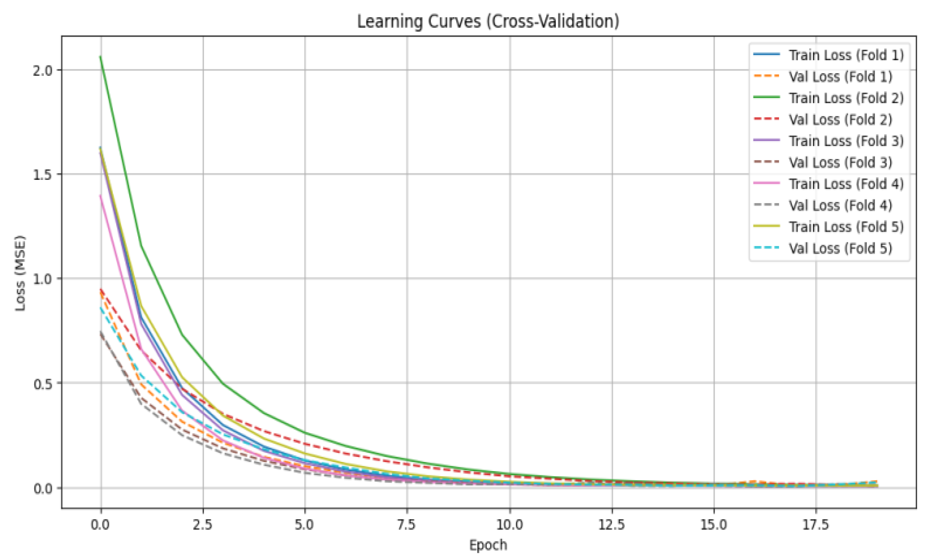
The learning curves derived from the five-fold cross-validation of the proposed CNN-LSTM model with an attention mechanism demonstrate robust performance and effective generalization for electricity demand forecasting, as illustrated in Figure 5. The implementation of early stopping, with a patience of 5 epochs, successfully halted training around 10–15 epochs, preventing overfitting and ensuring stable validation loss across all folds. The close alignment between training and validation losses, facilitated by regularization techniques such as dropout, L2 regularization, and batch normalization, underscores the model’s ability to capture the inherent seasonality and trends in electricity demand without memorizing noise.

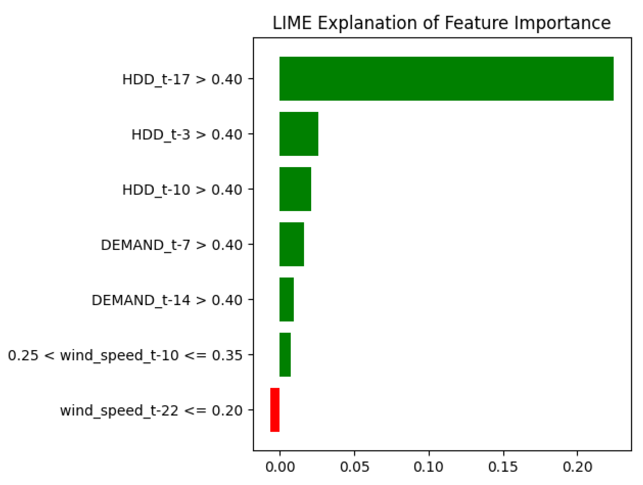
In this study, we leveraged LIME (Local Interpretable Model-Agnostic Explanations) to identify the most influential input parameters affecting our model’s decisions. The feature importance visualization shown in Figure 6 highlights the key variables that contributed the most to the predictions, providing a clear understanding of their impact on electricity demand forecasting.

The LIME feature importance analysis for the electricity demand prediction at a randomly selected timestamp, derived from the CNN-LSTM-Attention model, reveals the primary factors shaping this single instance, as presented in Figure 6. The HDD emerges as the most influential, with the HDD at a 17-day lag (HDD_t-17 > 0.40) exhibiting the greatest positive contribution (weight ≈ 0.225), followed by HDD_t-3 (>0.40, ≈0.026) and HDD_t-10 (>0.40, ≈0.021). These results underscore the pivotal role of temperature-related features across various lags in driving the demand forecast for this specific case. Furthermore, prior demand values at lags of 7 and 14 days (DEMAND_t-7 > 0.40, ≈0.016; DEMAND_t-14 > 0.40, ≈0.009) positively influence the prediction, highlighting the model’s dependence on historical demand trends for this timestamp. Wind speed features display opposing effects: moderate wind speed at a 10-day lag (0.25 < wind_speed_t-10 ≤ 0.35, ≈0.007) boosts the predicted demand, while low wind speed at a 22-day lag (wind_speed_t-22 ≤ 0.20, ≈−0.006) exerts a minor negative impact. These results highlight the model’s strength in integrating diverse temporal and meteorological inputs, with the HDD and lagged demand emerging as dominant predictors. This interpretability, grounded in the feature importance analysis, enhances the model’s reliability and practical value for electricity demand forecasting, demonstrating its capacity to model complex real-world dynamics.

The proposed CNN-LSTM with attention model substantially enhances electricity demand forecasting accuracy compared to the baseline CNN-LSTM model, demonstrating the value of incorporating an attention mechanism to capture intricate temporal dependencies. This improvement, however, comes at a significant computational expense. Training the proposed model on a dataset of 8000 samples using Google Colab with a GPU is markedly more time-intensive than training simpler architectures. For instance, the CNN-LSTM-Attention model, with 1,630,047 parameters, required approximately 50 min to train with a batch size of 128 and 500 epochs, achieving a MAPE of 1.69%. In contrast, the baseline CNN-LSTM model, with 1,307,343 parameters, completed training in 30–45 min under the same conditions, yielding a MAPE of 1.88%. Less computationally intensive models, such as the DNN with 45,000 parameters (training time: 5 min), the standalone CNN with 301,319 parameters (training time: 5–15 min), and the DNN-LSTM with 150,000 parameters (training time: 10–15 min), demanded significantly fewer computational resources. This trend reflects the increased complexity introduced by combining convolutional layers, recurrent LSTM units, and an attention mechanism, which collectively elevate processing demands. Despite the prolonged training duration, the superior predictive performance of the proposed model justifies its computational cost, particularly in applications where precision in electricity demand forecasting is critical. These findings highlight a key trade-off: while simpler models offer faster training and lower resource requirements, the CNN-LSTM with Attention model delivers enhanced accuracy, making it a compelling choice for scenarios prioritizing forecast reliability over computational efficiency.

4. Conclusions

This paper proposed a novel deep learning model that combines CNNs and LSTM networks with an attention mechanism to predict electricity demand in NSW. The forecasting results indicated that the proposed model outperforms other models, achieving the lowest MAE and MAPE among two individual models (CNN and DNN), and four hybrid models (DNN and CNN, DNN and LSTM, CNN and LSTM, CNN and LSTM with attention). This hybrid architecture offers a promising approach for electricity demand prediction, potentially leading to better electricity management and cost savings. This study is the first to utilize a CNN-LSTM model with an attention mechanism for forecasting electricity demand, leveraging HDD and CDD data specific to NSW, Australia, during the years 2020 through 2023.

Future research could incorporate additional weather variables, expand the model’s application to diverse geographical regions, and evaluate its performance on multi-year data to gain a deeper understanding of seasonal trends and long-term fluctuations in electricity demand. We also plan to explore emerging technologies, including probabilistic forecasting and advanced Transformer-based models like the TFT or Informer, which have become increasingly influential in time series processing. Moreover, future studies could examine optimization strategies for this model, such as implementing distributed training, to reduce its computational burden while preserving its prediction capabilities.