Fairness Criteria in Multi-Agent Systems: Optimizing Autonomous Traffic Management Through the Hierarchical Stackelberg Strategy

Abstract

As urban traffic density and congestion increase, effective urban traffic management becomes increasingly challenging, negatively impacting travel times and the overall efficiency of transportation systems. In this paper, a hierarchical Stackelberg model is presented to address both priority for emergency vehicles (EVs) and fairness for other vehicles. This model involves the Traffic Management Center (TMC) as the top-level authority, with emergency vehicles as the first-level leaders and regular vehicles (RVs) as the second-level followers. The multilevel decision-making structure enables real-time adjustments to prioritize critical traffic and ensure equitable treatment for regular traffic. Simulations were conducted under various traffic scenarios, including normal conditions, emergency vehicle priority, and peak traffic congestion. According to the results, the hierarchical Stackelberg model outperforms traditional models in terms of reducing average travel time, waiting time, and congestion. The model also incorporates fairness metrics such as Gini coefficients and skewness to ensure that regular vehicles are not disproportionately affected by emergency vehicle priority. According to these findings, the hierarchical Stackelberg model improves both traffic efficiency and fairness in complex urban environments, positioning it as a promising solution.

1. Introduction

Traffic management is a challenge for modern cities due to urbanization, which has increased vehicle density and resulted in frequent traffic jams, which negatively affect travel time and transportation efficiency. Traffic systems are complex, especially in urban areas with high traffic volumes, and require sophisticated control mechanisms that adapt dynamically to real-time conditions. With the aim of reducing delays, reducing congestion, and improving traffic flow through intersections, traffic signal optimization and vehicle traffic routing have become major research areas [1]. Stackelberg games, which treat traffic control as a problem of leadership and followers, have been shown to be effective in solving some of these challenges. This model equates central traffic management with a leader, while vehicles act as followers, adjusting routes and behaviors based on traffic signals and conditions set by the leader.

Over the past decade, game theory models—especially Nash and Stackelberg’s formulations—have gained interest in traffic control due to their ability to model competitive and hierarchical decision-making. Ref. [2] investigated the Nash/Stackelberg Q-learning model for traffic at a single intersection. Although the framework of reinforcement learning has been adapted to dynamic traffic conditions, the model remains limited to isolated small-scale environments and lacks scaling for multi-agent traffic control across cities. Furthermore, the lack of fairness guarantees led to a biased signal allocation, which adversely affected non-prioritized agents. Ref. [3] proposed a deep Q-network (DQN) method for controlling large-scale traffic signaling based on Nash equilibrium. The model addressed the computational flexibility of large networks but neglected priority differentiations such as emergency vehicles (EVs) and did not consider the level of equitable collaboration between agents or across intersections. Ref. [4] used the Nash and Stackelberg formulations on the real road network in Warsaw to verify them based on empirical data. However, the lack of static modeling of driver behavior and hierarchical priority for important agents, such as EVs, has revealed deficiencies in dynamic traffic allocation and fairness maintenance. Ref. [5] introduced the Nash–Stackelberg–Nash (NSN) game to integrate traffic and energy networks. Their model dealt well with system-level coordination but gave priority to economic efficiency over real-time response, making it inappropriate for traffic situations that require rapid reconfiguration, such as emergency situations or peak traffic congestion. Ref. [6] explored various game structures, including Nash, Stackelberg, and hybrid control. Although theoretically robust, this work lacked a comprehensive vehicle priority management strategy and fairness assurance strategy, making it not practical for heterogeneous urban traffic. Ref. [7] developed a Nash–Stackelberg planner that was adapted to multi-vehicle racing. The model has successfully handled aggressive maneuvers and priority-oriented tactics, but it is highly domain-specific and cannot be transferred to urban traffic management, where shared resources and fairness dominate. Ref. [8] presented a strategy-focused interaction algorithm with real traffic data, incorporating Stackelberg logic. Although their approach captures real-world dynamics, the model lacks system-level fairness restrictions and shows unstable behavior under unbalanced demand conditions.

Despite significant advances, existing models often fail in several critical areas. Many approaches give priority to efficiency, such as reducing travel time, but do not include fair considerations, leading to unfair access and allocation of resources. Others lack hierarchical differentiation, treat all vehicles the same way, and therefore neglect the priority of emergency routing. In addition, many models show limited scalability and struggle with coordination when facing dynamic, high-load, or emergency conditions. The proposed hierarchical Stackelberg Fairness Model addresses these limitations directly. It introduces a multi-tier decision-making framework that separates the strategic role of the Traffic Management Center (TMC) from the individual vehicle level. By incorporating fairness constraints measured with Gini coefficients and skewness into the optimization process, the model guarantees fair results. In addition, it includes a dynamic priority processing system that allows emergency vehicles (EVs) to adjust their route in real time while maintaining the regular vehicles (RVs)’ balance flow. This structure improves both scalability and adaptability, enabling effective performance at different traffic densities and operational demands.

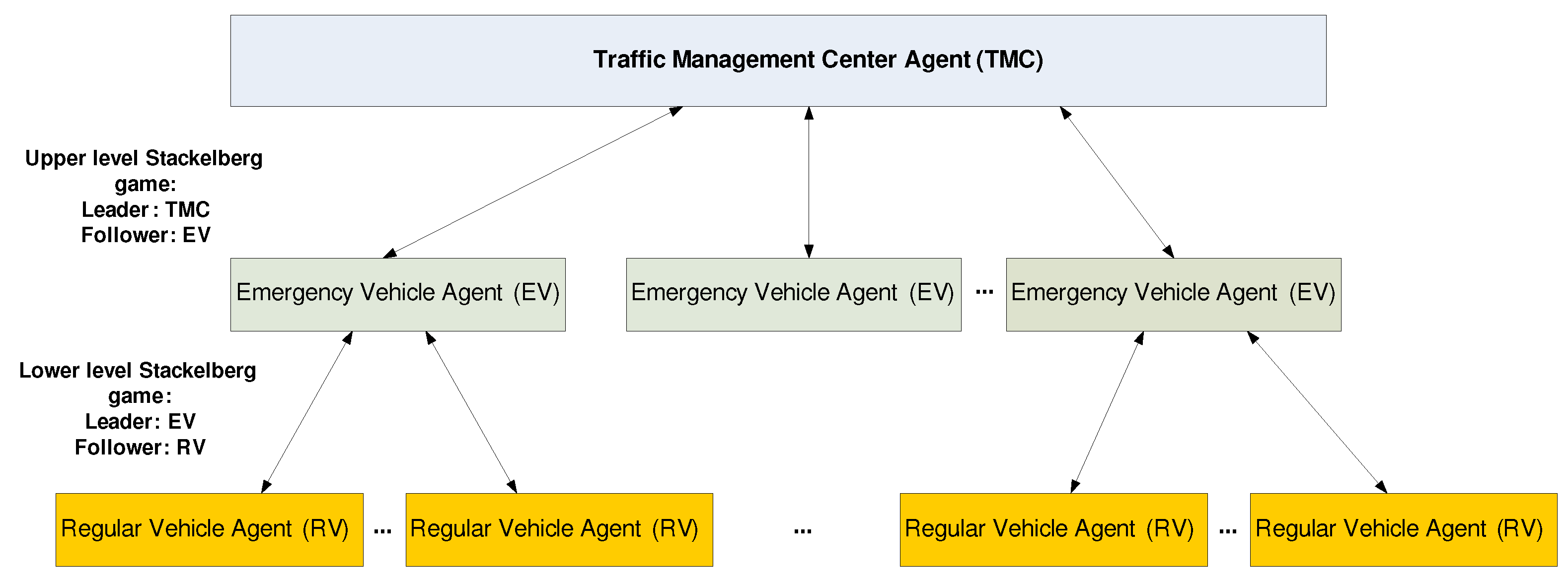
The paper proposes a hierarchical Stackelberg model for traffic management, which extends the traditional framework with multiple decision-making levels. Using this model, the Traffic Management Center (TMC) sets traffic signals and routing priorities as the top-level leader. A first-level follower is an emergency vehicle that receives priority within the network, while a second-level follower is a regular vehicle that adjusts their route according to emergency vehicle decisions and traffic control strategies. As a result of this hierarchical structure, we can control traffic more precisely, particularly in scenarios where emergency vehicles deserve priority while minimizing the delays of regular traffic and ensuring fairness.

This is the first study to explore traffic management using a hierarchical Stackelberg approach. In previous studies, the Stackelberg model was used mainly without indicating vehicle types or traffic flows. On the contrary, our hierarchical approach allows more flexibility and efficiency in dealing with complex traffic situations, even in highly congested urban areas where different levels of traffic priority must be balanced. Previous studies have widely adopted Nash and Stackelberg’s formulations for traffic management, including the optimization of isolated intersections [2], deep- reinforcement learning for signal control [3], and urban implementation in the real world [4]. Other works include autonomous vehicle control [6] and vehicle racing scenarios [7] in game theoretical frameworks. However, none of these studies implemented a hierarchical Stackelberg architecture that explicitly separated the decision-making layers (such as traffic management centers and individual agents), integrated fairness metrics, and dynamically reconfigured signal priorities in emergency and congestion scenarios. To the best of our knowledge, this is the first study to develop urban traffic control using a Hierarchical Stackelberg game incorporating multi-agent fairness constraints and real-time emergency responses.

Based on our simulations, we demonstrate that the Hierarchical Stackelberg model outperforms conventional models in terms of reduced travel times, shorter queues, and improved fairness in traffic management. The current model abstracts certain elements of the real-world traffic layout for clarity and computational feasibility but still captures the structural dynamics of signals-controlled urban intersections. This abstraction enables us to focus on assessing the effectiveness of the proposed decision-making mechanism (the hierarchical Stackelberg model) under controlled and interpretable conditions. In addition, the simplified layout retains key features that represent real intersections, such as directional lane and multi-agent interaction. Our main goal at this stage is to validate the fundamental algorithm behavior and assess its efficiency in the process of priority-based scenarios.

As for the rest of this paper, it is organized as follows: Section 2 provides a review of related literature on traffic control and game theory approaches. In Section 3, we explain the theoretical foundation for our Hierarchical Stackelberg model. In Section 4, the experimental setup is described, the results are discussed, and the proposed model is compared with existing approaches. Lastly, Section 5 concludes the paper and discusses future research directions.

2. Related Work

In several studies, biologically inspired algorithms have been used to optimize traffic. According to [9], dynamic vehicular traffic control systems can improve traffic management by reducing congestion through ant colony optimization (ACO) and traffic light optimization.

Machine learning and graph-based neural networks have been used to improve traffic-flow forecasting. Ref. [10] researched traffic-flow distribution forecasting in transport networks, presenting statistical methods for predicting vehicular distribution. To prevent traffic congestion zones, ref. [11] used a resilience-based approach, integrating vulnerability analysis of transportation systems. However, ref. [12] forecast traffic flow using graph convolutional neural networks (GCNs ) and branch-and-bound optimization, achieving high predictive accuracy, while [13] used spatial-temporal GCNs for real-time traffic forecasting, applying long-term short-term fusion. Through the application of deep learning and graph-based networks, these methods demonstrate the potential of traffic-flow forecasting to improve urban mobility systems through accurate forecasting [14].

Despite the value of accurate forecasting, we make our contribution by adapting traffic signals and routes in real time rather than relying only on predictive models. As a result of incorporating Stackelberg games into traffic control, we ensure a more dynamic and responsive system that can adjust in real time rather than just forecasting.

For adaptive traffic signal control, reinforcement learning has emerged as a key technique. A study [15] pioneered the use of deep reinforcement learning to optimize traffic signal timing, minimizing delays and improving the overall flow of traffic. Ref. [16] applied deep reinforcement learning to vehicular networks for traffic light control, further improving efficiency by learning dynamic traffic patterns. In their study of deep learning and discrete reinforcement learning, [17] emphasized the benefits of DRL for determining traffic signals. The study [18] examined reward definitions for reinforcement learning, which are crucial to adaptive signal control. As a result of these contributions, reinforcement learning can be used to create efficient and responsive traffic systems.

Although reinforcement learning (RL) has proven effective for adaptive signal control, our model relies on game theory (Stackelberg games). We incorporate hierarchical prioritization into traffic signal control, making the system responsive to emergency and regular vehicles, whereas traditional RL methods only optimize signal timings based on traffic flow.

Stackelberg and multi-agent games have been important in the development of traffic management strategies. A study [19] investigated socially aware multi-agent learning, which takes into account vehicle interactions and optimizes traffic outcomes. In [20], graph attention neural networks were applied to multi-agent game abstraction, which made it possible for agents to make more effective decisions together. Ref. [21] also studied consistent neighborhood cognition through cooperative learning in multi-agent reinforcement learning (MARL).

As opposed to multi-agent reinforcement learning (MARL), which emphasizes decentralized learning and agent cooperation, our model applies a Hierarchical Stackelberg game structure that explicitly distinguishes between leaders (Traffic Management Centers and Emergency Vehicles) and followers (Regular Vehicles). As opposed to MARL models, which generally lack explicit prioritization mechanisms, this hierarchical structure is better suited for transportation systems where prioritization is crucial, such as emergency vehicle routing.

Traffic congestion has also been modeled and resolved using game theory. According to [22], game-theoretic models have been shown to reduce traffic congestion by applying Stackelberg routing to parallel networks. According to [23], noncooperative transportation can be solved by linear generalized Nash games. The authors [24] distinguish between pure, mixed, and stochastic Nash equilibrium. Through cooperative and competitive strategies, their work provides insights into how congestion and traffic distribution can be managed.

In contrast with other game-theoretic models used in route planning, our model prioritizes emergency vehicles while maintaining overall network efficiency through Stackelberg games. Our approach incorporates hierarchical fairness mechanisms to ensure regular vehicles are not disproportionately affected by the prioritization of emergency traffic, as opposed to Nash equilibrium or pure Stackelberg games. Furthermore, we focus on real-time adaptive control rather than static route optimization.

Congestion pricing is another area in which game theory has been applied. As a means of managing traffic across multiple regions in transportation networks, [25] propose cooperative and competitive congestion pricing schemes based on Stackelberg games. In these models, network efficiency is balanced with revenue generation. The Stackelberg game model was extended by [26], incorporating option theory to optimize intermodal freight pricing strategies [27].

Instead of focusing on congestion pricing or competitive pricing strategies, our work focuses on real-time control and fairness-based decision-making within a hierarchical traffic management system. We use a game-theoretic framework rather than price incentives to manage congestion, ensuring that emergency vehicles receive priority while all road users are kept fair.

The combination of Nash and Stackelberg games has been explored in the planning of traffic routes and the control of traffic signals. Using Nash/Stackelberg Q-learning for traffic routes, [2] demonstrates how hybrid game models can optimize intersection traffic. In addition, [28] applied Nash game-based distributed control to balance traffic density across freeway networks, improving traffic-flow management significantly.

Although existing studies have employed Nash and Stackelberg games for traffic control, our innovation lies in the hierarchical Stackelberg model, which introduces multiple levels of decision-making, namely the Traffic Management Center (TMC) as leader, emergency vehicles as first-level followers, and regular vehicles as second-level followers. Compared to conventional Stackelberg models, this hierarchical structure is more effective at handling emergency traffic scenarios. Fairness measures are also implemented, ensuring that regular traffic does not experience excessive delays despite emergency traffic being prioritized.

To the best of our knowledge, this study is the first to investigate traffic congestion management using a hierarchical Stackelberg model. While numerous studies have explored traffic control using the standard Stackelberg framework, our contribution extends this by introducing a hierarchical structure, wherein decision-making occurs at multiple levels to better prioritize traffic. The results obtained from our model demonstrate its superiority over simpler Stackelberg approaches, showcasing improved efficiency and performance in managing both congestion and priority traffic scenarios.

3. Hierarchical Stackelberg Game Model for Traffic Management

In Figure 1, vehicles are represented by color-coded blocks at four traffic intersections: North, South, East, and West signals. Traffic flow is organized by designating lanes for left turns (LL), straight movements (SL), and right turns (RL). A red block represents an emergency vehicle positioned in the right lane (RL) at the South signal, indicating that in a real-world scenario, traffic management systems will prioritize its movement to facilitate quick navigation. In this diagram, multiple signals control the flow of vehicles in an urban traffic setting, ensuring that different lanes receive appropriate signals to proceed accordingly.

The current model abstracts certain elements of the real-world traffic layout for clarity and computational feasibility but still captures the structural dynamics of signals-controlled urban intersections. This abstraction enables us to focus on assessing the effectiveness of the proposed decision-making mechanism (the hierarchical Stackelberg model) under controlled and interpretable conditions. In addition, the simplified layout retains key features that represent real intersections, such as directional lane and multi-agent interaction. Our main goal at this stage is to validate the fundamental algorithm behavior and assess its efficiency in the process of priority-based scenarios.

There are three key components of the Hierarchical Stackelberg Game Model for Traffic Management: the Traffic Management Center (TMC), Emergency Vehicles (EVs), and Regular Vehicles (RVs). A TMC acts as a central authority for regulating and coordinating traffic flow, similar to a traffic control system used by cities. EVs, such as ambulances and fire trucks, are the system’s high-priority agents (leaders) that must reach their destinations quickly. Priority is given to these vehicles over regular traffic, which influences optimal routing. RVs, as lower-priority agents (followers), adjust their routes and speeds based on decisions made by emergency vehicles and the TMC, ensuring efficient and coordinated traffic management.

With a Stackelberg traffic management system, the Traffic Management Center (TMC) would prioritize certain lanes based on traffic flow. Depending on the signal changes, the vehicles would adjust their actions.

Figure 2 depicts a hierarchical Stackelberg game model for traffic management, focusing on the interaction between the Traffic Management Center (TMC), the Emergency Vehicle Agents (EV), and the Regular Vehicle Agents (RV). Two levels of Stackelberg games are represented in the diagram at different levels of the decision-making hierarchy. Similarly, emergency vehicles ensure that regular vehicles can move through traffic efficiently around them. While maintaining a smooth traffic flow, the hierarchical Stackelberg game structure balances the needs of emergency and regular vehicles.

By coordinating signal management, such a hierarchical decision-making model can help demonstrate its efficiency.

Two levels are involved in the game. At the higher levels, the Traffic Management Center (TMC) acts as the leader, while Emergency Vehicles (EVs) follow. For traffic management modeling, the TMC considers several variables, such as the vehicle’s position on the x- and y-axes, speed, orientation angle, direction of approach (left, center, right), intended path (right turn, straight turn, left turn), and intersection branch (North, South, East, West). To minimize EV travel times, the TMC sets dynamic signal timings and route priorities for EVs to ensure they follow the fastest routes. In the lower levels of the game, emergency vehicles (EVs) lead, and regular vehicles (RVs) follow. EVs determine their routes and signal them to the TMC, while RVs adjust their routes accordingly, maintaining a balance between their own travel times and EV priority.

4. Algorithm Overview

The adapted algorithm consists of a two-level hierarchical Stackelberg game, where the Traffic Management Center (TMC) acts as the upper-level leader and Emergency Vehicles (EVs) serve as the lower-level leaders. Regular Vehicles (RVs) are the followers that respond to the strategies set by the TMC and EVs.

4.1. Upper-Level Decision

To optimize signal time and determine EV route priorities, TMC uses input data, including traffic conditions, EV locations, and RV locations. Based on current traffic conditions, the estimated travel time for EVs and RVs is calculated. Once the priority level for each segment of the route is determined, the system gives priority to those who minimize the time of EV travel. To ensure smoothness and speed, traffic signals along the EV route are adjusted to create a “green wave” effect. Therefore, traffic signals and priority routes are updated accordingly, allowing EVs to move faster and more efficiently.

Objective for TMC: Maximize the combined objective function using Equation (1).

$$U_{\mathrm{TMC}}=\beta \times \left(\mathrm{Priority}\mathrm{EV}\mathrm{Success}\mathrm{Rate}\right)-\alpha \times \left(\mathrm{Total}\mathrm{Delay}\right)-\gamma \times \left(\mathrm{Fairness}\mathrm{Penalty}\right)$$

(1)

where: $\alpha ,\beta ,\gamma$ are the weights assigned to different objectives (minimizing delay, maximizing EV success, and ensuring fairness).

The fairness penalty measures the inequality in the distribution of road resources (lanes and signal priority) between emergency and regular vehicles.

The TMC’s utility function $U_{\mathrm{TMC}}$ aggregates rewards (EV success) and penalties (delays, fairness violations) to be maximized.

4.2. Lower-Level Decision

4.2.1. Emergency Vehicle Process Overview

The EV receives updated traffic signal times and route priorities from the Traffic Management Center (TMC). EVs use this information to evaluate routes considering updated signal times, such as dedicated routes or green waves. The aim is to select routes that minimize travel time and maximize the use of priority routes. Once the optimal route is determined, the EV communicates it to the TMC for coordination and traffic-flow optimization.

Objective for EVs: Maximize the utility function using Equation (2).

$${\mathrm{U}}_{\mathrm{EV}}=-\delta \times ({\mathrm{Delay}}_{\mathrm{EV}})+\zeta \times (\mathrm{Traffic}\mathrm{Rerouting}\mathrm{Efficiency})$$

(2)

where:

• $\delta$ is the weight for minimizing the emergency vehicle’s delay.
• $\zeta$ captures the effectiveness of rerouting regular vehicles to clear the path for the EV.

4.2.2. Regular Vehicle Process Overview

RVs receive input from EVs regarding EV decisions, traffic signals, and route priorities. The RV adjusts its route and speed based on priority routes for EVs and traffic signal conditions using this information. RV route selection is based on minimizing travel time while avoiding conflicts with priority EV routes. The congestion costs are also considered, and the speed is adjusted to maintain smoother traffic flows without affecting the priority EVs.

Objective for RVs: Maximize the utility function using Equation (3).

$${\mathrm{U}}_{\mathrm{RV}}=-\theta \times ({\mathrm{Delay}}_{\mathrm{RV}})+\kappa \times (\mathrm{Rerouting}\mathrm{Penalty})$$

(3)

where:

• $\theta$ represents the weight for minimizing the regular vehicle’s delay.
• $\kappa$ accounts for the inconvenience or penalty imposed by rerouting regular vehicles to prioritize emergency vehicles.

4.3. Algorithm Overview

The Hierarchical Stackelberg Fairness Algorithm (Algorithm 1) implements a Stackelberg-based fairness mechanism for traffic management involving emergency vehicles (EVs) and regular vehicles (RVs). This algorithm is designed to dynamically balance the needs of both types of vehicles using a hierarchical decision-making approach. The hierarchical Stackelberg algorithm iteratively maximizes the utility functions of the TMC, EVs, and RVs, balancing competing objectives through weight adjustments.

Algorithm 1 Hierarchical Stackelberg Fairness Algorithm

1: Initialize road network, traffic signals, vehicle positions 2: Set initial utility function weights (alpha, beta, gamma, delta, lambda, mu) 3: while traffic is active do 4:     Input real-time traffic data 5:     Update road network state 6:     // Upper-Level Decision: TMC Optimization 7:     Calculate expected travel times for EVs and RVs 8:     Determine route priorities for minimizing EV travel time 9:     Optimize traffic signals for “green wave” effect 10:     Output updated signal timings and priorities 11:     // Lower-Level Decision: EV and RV Strategy Optimization 12:     for each EV do 13:         Evaluate route options based on updated signal timings 14:         Choose a route that minimizes travel time and maximizes priority 15:         Output optimal route choices to TMC 16:     end for 17:     for each RV do 18:         Adjust route and speed based on EV decisions and signal states 19:         Choose a route that minimizes travel time and avoids conflicts 20:         Output adjusted routes and speeds 21:     end for 22:     // Evaluate Fairness 23:     Calculate Gini coefficient for travel times 24:     Calculate skewness for travel time distribution 25:     if fairness constraints are not met then 26:         Adjust signal timings and route priorities 27:         Continue optimization loop 28:     else 29:         Break 30:     end if 31: end while

A Stackelberg-based fairness mechanism is implemented using a hierarchical decision-making framework, dynamically prioritizing EVs while maintaining fair and efficient traffic flow for RVs. Iterative optimization ensures that fairness metrics, such as the Gini coefficient and skewness, are kept within acceptable limits, which enables all road users’ needs to be met.

The Gini coefficient is calculated by combining the average travel times of EVs (emergency vehicles) and RVs (regular vehicles) into one dataset and using a similar approach to calculate waiting times. Let ${\mathrm{T}}_{EV}$ be the EV travel time and ${\mathrm{T}}_{\mathrm{RV}}$ be the RV travel time. In the next step, these values are sorted ascending. The cumulative proportion of travel and waiting times is calculated for each value ${\mathrm{X}}_{\mathrm{i}}$ in the sorted data. Using Formula (4), we can calculate the Gini coefficient:

$$G={\displaystyle \frac{{\sum }_{i=1}^n{\sum }_{j=1}^n\left|X_i-X_j\right|}{2n^2\overline{X}}}$$

(4)

where ${\mathrm{X}}_{\mathrm{i}}$ and ${\mathrm{X}}_{\mathrm{j}}$ are individual travel or waiting times, n is the total number of data points (both EVs and RVs), and $\overline{X}$ is the mean of the travel or waiting times. The Gini coefficient, which ranges from 0 (perfect equality) to 1 (maximum inequality), measures the disparity between the two groups. In the context of traffic management, it indicates how fairly resources, such as signal timing, are distributed between emergency and regular vehicles.

Calculating Skewness

The skewness of a distribution helps determine whether the distribution of travel times or waiting times is symmetrical, positively skewed (indicating a longer tail on the right), or negatively skewed (indicating a longer tail on the left). To calculate skewness, the first step is to calculate the mean, where ${\mathrm{X}}_{\mathrm{i}}$ represents individual travel times, and n is the number of values. As a next step, the standard deviation is calculated to determine the degree of dispersion in the data. Finally, we calculate skewness using Formula (5):

$$\mathrm{Skewness}={\displaystyle \frac{1}{n}}\sum {\left({\displaystyle \frac{X_i-\mu }{\sigma }}\right)}^3,$$

(5)

where $\mu$ is the mean calculated as Formula (6):

$$\mu ={\displaystyle \frac{\sum X_i}{n}},$$

(6)

and $\sigma$ is the standard deviation calculated as Formula (7):

$$\sigma =\sqrt{{\displaystyle \frac{\sum {\left(X_i-\mu \right)}^2}{n}}}.$$

(7)

The interpretation of skewness is as follows: when skewness equals 0, the distribution is symmetrical; when skewness is greater than 0, the distribution is positively skewed with a longer right tail; and when skewness is less than 0, the distribution is negatively skewed with a longer left tail.

5. Simulation and Results

Firstly, the methods will be evaluated based on standard parameters defined as follows:

The average travel time represents the total time spent by all vehicles within the transport network, divided by the number of vehicles that have entered the simulation. This parameter is mathematically expressed in Equation (8) as:

$$\overline{t}={\displaystyle \frac{1}{N}}\sum _{i=0}^N\left(t_{i,\mathrm{end}}-t_{i,\mathrm{start}}\right)$$

(8)

where the variable $\overline{t}$ represents the average time calculated over a total of N vehicles. For each vehicle, i, $t_{i,start}$ denotes the start time, and this value is used alongside other time data to compute the overall average time for the vehicles within the traffic system, $t_{i,\mathrm{end}}$ is the end time for vehicle i. The relationship between these variables helps assess traffic flow and efficiency in the model.

The average waiting time Equation (9) is determined by dividing the total accumulated waiting time of all vehicles by the total number of vehicles in the system.

$$\overline{t_w}={\displaystyle \frac{1}{N}}\sum _{i=0}^N{t}_{i,w}$$

(9)

where the variable $\overline{t_w}$ represents the average waiting time across N vehicles, where $t_{i,w}$ is the specific waiting time for vehicle i. This metric is used to evaluate traffic efficiency and delays within the system.

Each lane’s queue length is determined by counting the number of halted vehicles within it. The statistical queue length can be calculated by adding the queue lengths across all lanes and dividing by the total number of lanes, resulting in a single value indicating the length of the network. Equation (10) describes how to compute this value:

$$q_l={\displaystyle \frac{{\sum }_{i=0}^{L}q{l}_i}{L}}$$

(10)

where the variable $q_l$ represents the average queue length across L lanes, where ${\mathrm{ql}}_{\mathrm{i}}$ is the specific queue length for lane i.

5.1. Multi-Objective Optimization of Traffic Signal Prioritization: Balancing Emergency Response, System Efficiency, and Fairness

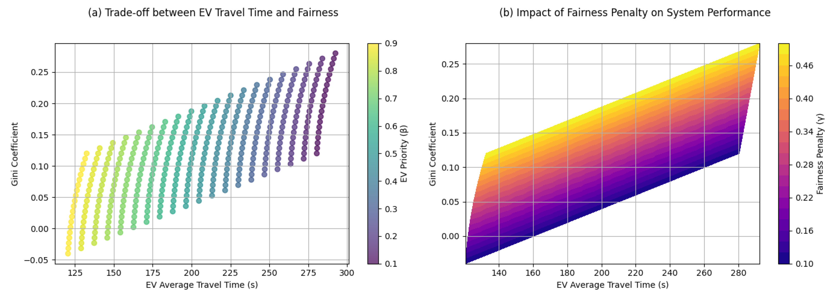
Figure 3 includes two subfigures to compare traffic signal optimization and traffic signal delay for EV travel time. Figure 3a Trade-off between EV Time and Fairness shows a distribution diagram where each point represents a simulation example, the x-axis indicates the average EV travel time in seconds, and the y-axis shows the Gini coefficient corresponding to the metric to quantify the fairness of the travel time distribution of all vehicles. Color gradient encodes EV priority weight ($\beta$). This graph shows that the lower travel time of EVs is generally associated with a higher value $\beta$, which means a better priority for emergency vehicles. However, with increasing and EV travel time declining, the Gini coefficient also tends to increase, indicating increased system unfairness. This demonstrates a trade-off where improving EV response times may lead to equity losses among regular vehicle users. Figure 3b accentuates this by presenting the values of the fairness penalty ($\gamma$) as contour levels on the same two variables: the EV travel time and the Gini coefficient. The contour map shows how varying $\gamma$ affects the system’s ability to balance performance and fairness. Lower $\gamma$ values dominate regions with longer EV travel times and an equal traffic flow (lower Gini), while higher $\gamma$ values appear in areas where fairness is compromised, indicating shorter EV periods. This supports the concept that $\gamma$ is a regulatory parameter and penalizes solutions that undermine fairness, even if they are beneficial to EV travel time. Collectively, these two subfigures illustrate the dynamic tension between efficiency and equity in traffic management and indicate that adjustment of weights ($\beta$ and $\gamma$) is required to achieve an appropriate balance based on operational objectives.

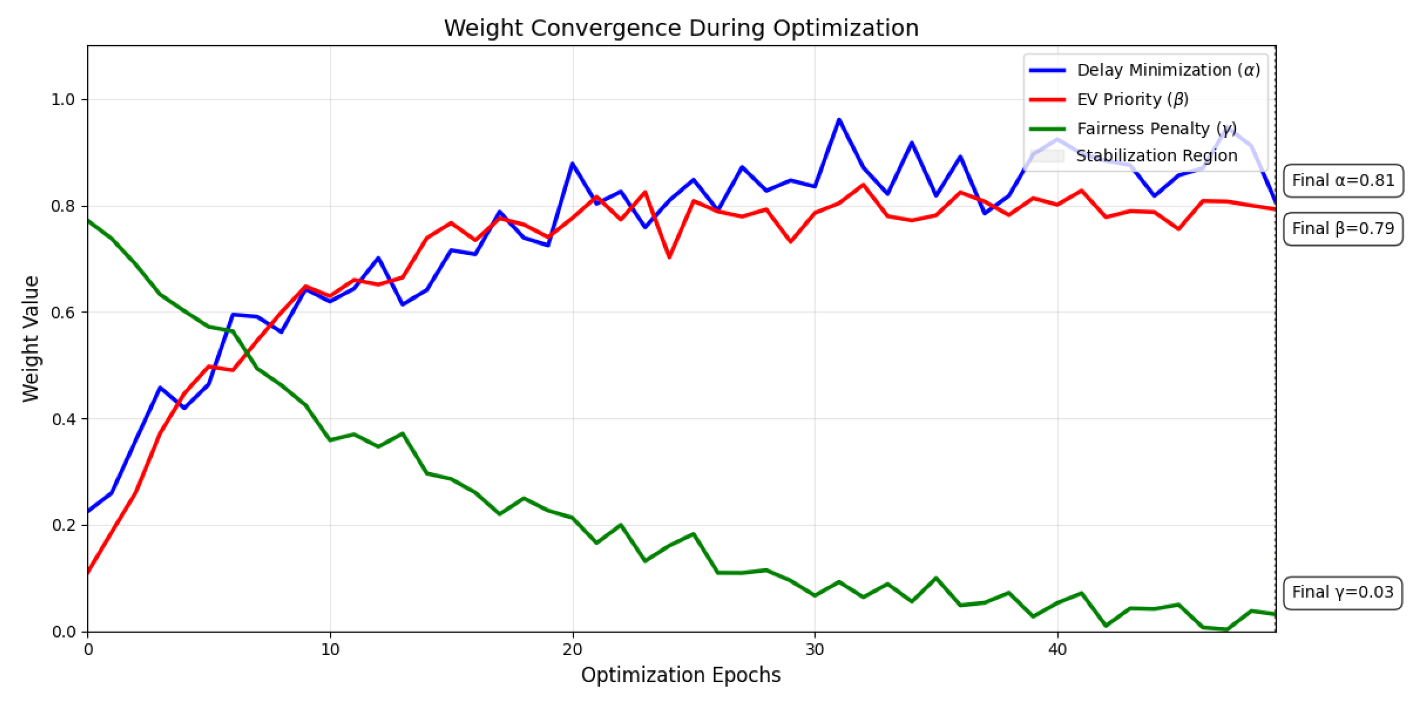
Figure 4 shows the evolution of optimization weights over 50 epochs. Initially, $\alpha$ (delay minimization) decreased rapidly from 0.9 to 0.25, while $\beta$ (EV priority) increased from 0.1 to 0.75 by the 30th epoch, highlighting the shift to priority for emergency vehicles. The fairness weight $\gamma$ gradually decreased from 0.8 to about 0.15, reflecting a reduction in the emphasis on fairness, as other objectives are at the forefront. Stabilization points are marked with vertical lines, and all weights converge within 30 epochs. The initial dynamics highlight a sharp increase in $\alpha$ and $\beta$, and a steady decline in $\gamma$. These convergence models show that the optimization process has succeeded in navigating the differences between competing objectives. The final weight distribution (moderate $\alpha$, high $\beta$, low $\gamma$) implies that the system prioritizes emergency vehicles while accepting some delays for regular traffic, with relatively relaxed fairness constraints. All parameters are stable within 30 epochs, showing efficient convergence.

The practical values of parameters $\alpha$ (delay reduction), $\beta$ (emergency vehicle priority), and $\gamma$ (fairness penalty) must be determined in relation to specific operational contexts, policy priorities, and dominant traffic dynamics. In the case of delay minimization parameter $\alpha$, a value between 0.5 and 0.7 is generally recommended. This emphasizes the overall efficiency of the network and is particularly suitable in situations where congestion management is important, but there is no immediate need for emergency vehicles (EVs). When the efficiency of the entire system is a priority, $\alpha$ should be relatively high.

The parameter $\beta$, which controls the priority of emergency vehicles, is best kept between 0.2 and 0.5 in normal traffic operations. In emergency situations, however, $\beta$ should be increased considerably and could reach values between 0.6 and 0.9. This ensures that EVs receive sufficient priority without unnecessarily disrupting regular traffic in emergency situations. The fairness penalty parameter $\gamma$ is usually selected between 0.1 and 0.4. A higher $\gamma$ reflects a stronger emphasis on an equitable distribution of resources, minimizing the differences in travel time between different types of vehicles. This is especially relevant in urban environments where social equity or public transport vehicles (such as buses) are part of the traffic ecosystem. However, in emergency situations where the priority routing is more important, $\gamma$ should be reduced to prevent it from reversing the priority expected. Under regular traffic conditions, parameters such as $\alpha$ = 0.6, $\beta$ = 0.3, and $\gamma$ = 0.2 can be effective in maintaining a balanced balance between network efficiency, emergency preparedness, and fairness. On the other hand, in emergency scenarios where emergency vehicles (EVs) need priority routing, weights are adjusted to emphasize response by adjusting $\beta$ to 0.8, reducing $\gamma$ to 0.1, and moderate $\alpha$ to about 0.4. In cases of severe congestion, when the stabilization of the overall network flow becomes important, higher priority is placed on the minimization of delay by setting $\alpha$ to 0.7, $\beta$ to 0.2, and $\gamma$ to 0.3. In contexts where equity considerations are of paramount importance, the Fairness component ( $\gamma$ = 0.4) is given more weight, and $\alpha$ and $\beta$ are properly adjusted to maintain system balance. These configurations reflect the adaptability of the model to various operational objectives and traffic environments. In adaptive systems, these parameters can be continuously adjusted with real-time feedback or reinforcement learning. However, initial calibration should be informed by simulations based on realistic traffic scenarios to ensure the effectiveness and robustness of the model in practical deployment.

5.2. Scenario Design and Network Specifications

The simulation scenario is based on hypothetical variations to test the robustness of our hierarchical Stackelberg model under different traffic conditions. These scenarios include normal traffic conditions, emergency vehicle priority situations, and peak congestion times. Normal condition scenario reflects the typical weekday traffic patterns during morning peak hours, while emergency priority scenarios simulate the network traffic flow of emergency vehicles. Peak congestion scenarios model high-density traffic with queues to evaluate system performance under pressure. The simulated urban subnet covers an area of 4 km² and represents mixed-use areas for commercial and residential activities. The network consists of 12 signal crossings and 24 bidirectional road segments. This configuration enables us to study the interaction between emergency vehicles and regular vehicles in a controlled but representative urban environment. The network includes three functional road classes: arterial, collector, and local access roads. Arterial roads make up 60% of the network, with a speed limit of 60 km/h and three routes in each direction. Collector roads account for 30%, 40 km/h speed limit, and two lanes per direction. Local access roads constitute the remaining 10% with a speed limit of 30 km/h and a lane per direction. The intersections are primarily signaled (12 of which are in total) using adaptive time-controlled active signals, while four unsigned intersections are modeled with priority rules. Traffic demand is synthesized to reflect real urban conditions. Origin Destination matrices (ODs) are constructed to represent baseline traffic flows, with peak time demand reduced to 120% of baseline to simulate congestion. Emergency vehicles are introduced at 5–10 vehicles per hour, representing 2% of total traffic flow, while regular vehicles are 1800–2400 vehicles per hour and vary by scenario. Turn ratios at intersections are set at 25% left, 50% straight, and 25% right to mirror typical urban traffic behavior.

Traffic Flow Modeling Assumptions

The speed-flow relationship used in our model is based on the Macroscopic Traffic-Flow Formula of Greenshields, which assumes a linear relationship between the vehicle speed (v) and the traffic density (k). This relationship is mathematically expressed as:

$$v=v_f\left(1-{\displaystyle \frac{k}{k_j}}\right)$$

(11)

where $v_f$ represents the free-flow speed (i.e., the maximum speed possible under low traffic density), $k_j$ represents the jam density (critical traffic density), and k represents the current vehicle density per unit length.

The formula allows a direct estimate of traffic flow (q) as the product of density and speed:

$$q=k·v_f\left(1-{\displaystyle \frac{k}{k_j}}\right)$$

(12)

With increasing density, the speed gradually decreases, eventually reducing the flow rate and simulating the beginning of congestion. The Greenshields model is chosen for its empirical relevance and analytical utility, especially in urban traffic systems, and is a standard reference in traffic engineering literature.

In terms of road capacity and free-flow speed, identifying the peak of the speed curve determines the maximum theoretical capacity of a road segment ($q_{\max }$), which is given by:

$$q_{\max }={\displaystyle \frac{v_f·k_j}{4}}$$

(13)

The capacity values are determined according to established standards such as the Highway Capacity Manual (HCM), which estimates about 1900 vehicles per hour per lane for urban arterials. These values were then refined by empirical adjustments, considering contextual factors such as traffic signal timing and pedestrian interference, based on local traffic surveys conducted at key intersections.

5.3. Simulation

We conduct a comparative analysis of the proposed Hierarchical Stackelberg strategy against two benchmark approaches: the baseline control model and the conventional Stackelberg model. This evaluation aims to assess the performance improvements introduced by incorporating hierarchical coordination mechanisms. Firstly, the baseline model represents a traditional fixed-time signal control system that does not give priority to emergency vehicles (EVs) and does not facilitate adaptive coordination. It serves as a reference point for assessing the value of game theory and hierarchical strategies. In the Stackelberg standard model, the Stackelberg single-level game also includes the Traffic Management Center (TMC), which acts as the leader, and the regular vehicle reacts as the follower. Although the model introduces interaction optimization, the vehicle types (e.g., EVs and RVs) do not differ, and its response is limited in priority scenarios.

5.3.1. Scenario 1: Normal Traffic Conditions

Scenario 1 shows normal and balanced traffic flow without extreme congestion or special priority requirements. This scenario reflects a moderate traffic flow where Regular vehicles (RVs) and occasional emergency vehicles (EVs) are available. Under these standard conditions, a smooth flow of traffic is the goal, with minimal waiting time and delays. In ideal steady-state traffic, this scenario provides a baseline for assessing the system’s performance.

Based on

Table 1. Comparison of EV and RV performance metrics under normal traffic conditions for three traffic management models.

Model	EV Average Travel Time (s)	EV Average Waiting Time (s)	RV Average Travel Time (s)	RV Average Waiting Time (s)	Average Queue Length (Vehicles)
Hierarchical  Stackelberg  Model	280	60	320	80	10
Standard  Stackelberg  Model	300	65	340	90	12
Baseline Model	350	80	380	110	15

, in the hierarchical Stackelberg model, emergency vehicles (EVs) had a waiting time of 60 s, a $25\%$ decrease compared to the basic model of 80 s. RVs also benefit from improved traffic flow and reduced wait times from 110 s to 80 s in the hierarchy model. Moreover, the hierarchical Stackelberg model significantly reduced intersection queues and congestion by $33\%$ compared to the baseline model, demonstrating its efficiency in managing emergency and routine traffic. Standard Stackelberg models have moderate improvements over baseline models, but they are less effective than hierarchy models, especially for RVs.

5.3.2. Scenario 2: Emergency Vehicle Priority

In scenario 2, emergency vehicles (EVs), such as ambulances or fire trucks, must be prioritized so that they can pass directly through the traffic network. As in a real-life emergency, the Traffic Management Center (TMC) must adjust the traffic signal time dynamically to prioritize EV traffic while minimizing disruptions to normal traffic flow. The objective is to identify whether the system reduces EV travel and waiting times and maintains a reasonable flow of regular vehicles (RVs) while managing to reduce EV travel and waiting times.

Based on

Table 2. Comparative performance of traffic control models under emergency vehicle priority conditions.

Model	EV Average Travel Time (s)	EV Average Waiting Time (s)	RV Average Travel Time (s)	Average Queue Waiting Time (s)	Length (Vehicles)
Hierarchical  Stackelberg  Model	150	20	350	100	11
Standard  Stackelberg  Model	200	40	380	120	14
Baseline  Model	300	80	450	150	25

, the hierarchical Stackelberg model significantly reduced the average travel time of emergency vehicles (EVs) to 150 s, a $50\%$ reduction compared with the basic model. In the case of regular vehicles, the average number of queues is significantly shorter, with 11 hierarchical models and 25 base models, reflecting a 56 percent improvement in congestion management. Even though the standard Stackelberg model improves the performance of emergency vehicles, it leads to longer waiting times and queues for regular vehicles due to the absence of hierarchical priority. Using a hierarchical model, emergency vehicles receive priority without exacerbating the flow of normal vehicles, which is critical in real emergency situations.

5.3.3. Scenario 3: Peak Traffic with Congestion

In Scenario 3, heavy traffic congestion occurs during rush hours, or there are major traffic delays. There is a high number of regular vehicles (RVs) at the intersection, resulting in bottlenecks. EVs may still require priority, but the main challenge is to manage increased traffic volumes without creating congestion or excessive delays. This scenario tests the system’s ability to efficiently manage high-density traffic, reduce queue lengths, maintain fair resource allocation, and prioritize EVs when necessary.

Based on

Table 3. Evaluation of traffic control strategies under peak congestion: Impact on emergency and regular vehicle performance.

Model	EV Average Travel Time (s)	EV Average Waiting Time (s)	RV Average Travel Time (s)	RV Average Waiting Time (s)	Average Queue Length (Vehicles)
Hierarchical  Stackelberg  Model	150	20	350	100	21
Standard  Stackelberg  Model	200	40	380	120	25
Baseline  Model	300	80	450	150	33

, the hierarchical Stackelberg model maintains an average line length of 25 vehicles, $44\%$ less than the 45 vehicles observed in the base model under high traffic conditions. Hierarchical priority also benefits emergency vehicles, reducing wait times from 200 s to 120 s. For regular vehicles, the hierarchical model has a 150 s waiting time, which is significantly better than the 250 s waiting time of the baseline model, reflecting a $40\%$ improvement in queue management. Standard Stackelberg models perform fairly well but lack the efficiency of hierarchy models, as their average line lengths are 30 vehicles instead of 25. It is demonstrated that the Stackelberg Hierarchical Model provides a better balance between emergency vehicles and regular traffic management, reducing congestion and maintaining fairness during peak traffic hours.

Based on the analysis, it is clear that the hierarchical Stackelberg model consistently outperforms other models in all scenarios and reduces emergency and regular vehicle travel times significantly. It prioritizes emergency vehicles efficiently, maintains fairness, avoids excessive delays in regular traffic, and manages congestion well, especially during peak hours. In comparison, Stackelberg’s standard model offers improvements over the base model but lacks the hierarchical structure required for optimal congestion management and priority setting. Baseline models consistently underperform, especially in emergency and high-volume situations, with longer travel times, ineffective congestion management, and long queues.

5.4. Interpretation

1.

Explicit priority and separation of objectives: the hierarchical structure allows a clear priority for the emergency vehicle (EV) while at the same time optimizing the route for the regular vehicle (RV). This decoupling ensures that the priority of EVs is not at the expense of excessive RV delays, as the Traffic Management Centre (TMC) dynamically balances the two objectives through utility functions (Equations (1)–(3)). Table 1, Table 2 and Table 3 show this balance, showing that the EV travel time has been significantly reduced (e.g., 50% of the improvement in Scenario 2) and that there has been no disproportionate increase in RV delays (e.g., only 33% of the RV wait time in Scenario 2 has been extended compared to 67% of baseline).

2.

Real-time adaptability: Hierarchy allows real-time adjustments by distributing decision-making between levels. For example, TMC acts as a global coordinator (upper level), and EVs and RVs react locally (lower level). This avoids the rigidity of single-level models where centralized control struggles to adapt to local emergency or congestion.

3.

Fairness through hierarchical feedback: The inclusion of fairness indicators (Gini coefficients, skewness) in the algorithm ensures that resource allocation is monitored and iteratively adjusted. The hierarchical structure fundamentally supports this, allowing the TMC to penalize unfair results (e.g., through the Fairness Penalty in Equation (1) and to redistribute signal timing or lane priority. This explains why all scenarios achieve the Gini values below (approximately 0) in the model compared to a non-hierarchical approach.

4.

Mitigation of conflict propagation: In the traditional Stackelberg or Nash model, conflicts between EVs and RVs often spread uncontrollably, leading to congestion. Hierarchical models mitigate this by limiting EV decisions to priority only critical routes, while RVs maximize the remaining resources. This is demonstrated in scenario 3 (peak congestion), where hierarchical models reduce queue length by 44% compared to baseline models, whereas standard Stackelberg models (lack of hierarchy) do not manage spillover effects as effectively.

6. Conclusions and Future Work

This study proposes a hierarchical Stackelberg model for traffic management to address the complex challenges of prioritizing emergency vehicles (EVs) while maintaining fairness and minimizing delays for ordinary vehicles (RVs). This approach extends the traditional Stackelberg framework by introducing a multilevel decision-making structure in which the Traffic Management Center (TMC) is the leader, followed by emergency vehicles as the first and regular vehicles as the second. A hierarchical traffic control structure is more effective in situations involving emergency vehicles. Based on the simulation results, the hierarchical Stackelberg model is superior to the traditional one. Across all traffic scenarios, including normal conditions, emergency vehicle priority, and peak traffic congestion, the model consistently reduces the average travel time and waiting time for emergency vehicles. By including fairness metrics like Gini and Skewness coefficients, regular vehicle delays remained within acceptable bounds, as reflected in fairness metrics if emergency vehicles were prioritized. This model improves overall traffic flow, reduces congestion, and addresses the often overlooked issue of distributing resources equally among different types of vehicles.

Critical direction for future research includes the inclusion of unexpected infrastructure disturbances such as bridge failures, accidents, and scheduled road closures [29,30]. These disturbances can have a significant impact on travel behavior and system reliability, thereby reducing network resilience. Included in this dynamic, the model would better capture the uncertainties of the real world and improve its operational application. Another promising extension is the explicit integration of road safety into the objective function of the model [31,32], in addition to efficiency and fairness. Safety has economic, social and ethical dimensions, and ignoring it can ignore critical aspects of system performance. The inclusion of penalties for crash risk could provide a more comprehensive assessment of traffic management strategies.