Solving Collaborative Scheduling of Production and Logistics via Deep Reinforcement Learning: Considering Limited Transportation Resources and Charging Constraints

Abstract

With the advancement of logistics technology, Automated Guided Vehicles (AGVs) have been widely adopted in manufacturing enterprises due to their high flexibility and stability, particularly in flexible and discrete manufacturing domains such as tire production and electronic assembly. However, existing studies seldom systematically consider practical constraints such as limited AGV transport resources, AGV charging requirements, and charging station capacity limitations. To address this gap, this paper proposes a flexible job shop production-logistics collaborative scheduling model that incorporates transport and charging constraints, aiming to minimize the maximum makespan. To solve this problem, an improved PPO algorithm—CRGPPO-TKL—has been developed, which integrates candidate probability ratio calculations and a dynamic clipping mechanism based on target KL divergence to enhance the exploration capability and stability during policy updates. Experimental results demonstrate that the proposed method outperforms composite dispatching rules and mainstream DRL methods across multiple scheduling scenarios, achieving an average improvement of 8.2% and 10.5% in makespan, respectively. Finally, sensitivity analysis verifies the robustness of the proposed method with respect to parameter combinations.

1. Introduction

With the continuous advancement of technology, intelligent manufacturing has emerged as a key approach to improving production efficiency, optimizing resource allocation, and enhancing market competitiveness—thereby promoting high-quality development in the manufacturing industry. As a core component of intelligent manufacturing, the job shop scheduling problem (JSP) [1] plays a crucial role in optimizing resource allocation, shortening production cycles, and controlling manufacturing costs.

Driven by increasingly customized and diversified production demands, flexible job shops have gained prominence. As an extension of traditional job shop scheduling, the flexible job shop scheduling problem (FJSP) allows operations to be assigned to multiple machines, each capable of processing different tasks [2]. This flexibility enables dynamic resource allocation and improves the shop’s ability to handle uncertain order requirements. However, this increased flexibility also introduces new challenges, particularly frequent job transfers between machines, thereby giving rise to complex intra-shop transportation issues. Traditionally, production scheduling and logistics scheduling in FJSPs have been addressed independently, overlooking the intricate coupling between processing machines and transport equipment.

As logistics technology evolves, AGVs have been widely adopted in manufacturing systems due to their high flexibility and operational stability. According to recent statistics, the global AGV market reached approximately USD 2.74 billion by the end of 2023, up from USD 1.86 billion in 2018, with a compound annual growth rate (CAGR) of 8.02%. In the same year, the global shipment of forklift AGVs—commonly used in manufacturing workshops—reached around 30,700 units, marking a year-over-year increase of 46.19% [3].

In real-world manufacturing scenarios, once an operation is completed on a machine, it must be transferred—often via AGVs—to the next designated machine or a storage buffer [4]. The subsequent operation can only commence once the processed part has been delivered to the area. This creates a strong interdependence between production scheduling and logistics scheduling. Therefore, production scheduling and logistics scheduling are intricately coupled in flexible job shops. However, most existing studies tend to ignore this coupling by investigating production scheduling [5,6,7] and logistics scheduling [3,8,9,10] independently, which often results in infeasible scheduling solutions in real-world applications [11].

In recent years, some researchers have begun exploring collaborative scheduling approaches that jointly consider production and logistics in FJSP environments. Nonetheless, most of these studies assume either unlimited transportation resources [12,13,14], like a sufficient number of AGVs or mobile robots, or fixed transfer times [15]. A few works have attempted to address limited AGV availability by designing case-specific AGV configurations for different problem scales [16,17]. Moreover, current research on the collaborative scheduling of production and logistics in flexible job shops is still in its infancy. Many practical factors have not been thoroughly addressed, such as the power consumption of AGVs, variations in transportation speed, charging strategies, and the availability of charging stations. In fact, such issues have already been well considered in other AGV-related application domains, such as port handling systems [18,19,20,21].

To fill these research gaps, this study investigates a flexible job shop production-logistics collaborative scheduling problem with limited transportation resources and charging constraints (FJSPLSP-LTCC). On top of machine and operation selection, the proposed model integrates AGV assignment for each transport task, taking into account battery depletion, in-transit charging requirements, and charger constraints. To ensure alignment with practical conditions, multiple scenarios with different shop sizes have been designed, each with limited AGV and charger resources. In addition, this study introduces the “deterioration” effect of AGVs: as the battery level decreases, the transportation efficiency declines, resulting in prolonged handling time. This assumption is based on engineering observations of AGV operation in industrial scenarios, where AGVs typically reduce their operating speed at lower battery levels to conserve energy or ensure operational safety. Although comprehensive empirical modeling data are currently lacking, the incorporation of this effect enhances the practical applicability of the proposed scheduling model and reflects the actual operating characteristics of AGVs. Future research will focus on collecting empirical data to further validate and optimize the model.

Heuristic algorithms [22,23,24] and Deep Reinforcement Learning (DRL) approaches [17,25] are commonly used to solve collaborative scheduling problems in flexible job shops. However, the problem addressed in this paper incorporates several additional decision dimensions—such as charging constraints—compared with traditional models, making it a high-dimensional scheduling problem. DRL, as a fully reactive scheduling method, leverages data to learn the correlation between data distributions and decision behaviors, and has demonstrated superior optimization performance in solving such high-dimensional and complex scheduling tasks [17,26,27]. Among DRL methods, PPO and its variants have gained significant attention in recent years for their robustness, stability, and ease of implementation [28,29,30,31,32]. Accordingly, this study develops a customized PPO-based DRL algorithm named CRGPPO-TKL to solve the FJSPLSP-LTCC. The algorithm samples candidate actions and computes candidate probability ratios to better evaluate policy divergence. Furthermore, it introduces a target KL divergence mechanism to dynamically adjust the clipping range, thus maintaining a balance between exploration and policy stability.

In summary, the main contributions of this study are as follows:

(1)

A comprehensive modeling framework for collaborative production-logistics scheduling in flexible job shops is proposed, which incorporates limited AGV resources, AGV charging constraints, and the deterioration effect between battery level and transportation speed, thereby enhancing the practical applicability of the scheduling model.

(2)

Multiple flexible job shop scenarios with varying workshop scales are designed, and a systematic analysis is conducted to determine the optimal AGV configuration for each layout, providing valuable guidance for resource allocation in practical applications.

(3)

An improved PPO algorithm—CRGPPO-TKL—is developed, which enhances action evaluation through candidate probability ratio sampling and dynamically adjusts the clipping range based on the target KL divergence, thereby improving learning stability and performance in solving complex collaborative scheduling problems.

The remainder of this paper is organized as follows: Section 2 reviews related literature on production-logistics collaborative scheduling in flexible job shops. Section 3 defines the proposed FJSPLSP-LTCC problem. Section 4 describes the developed DRL framework. Section 5 presents experimental results and analysis. Finally, Section 6 concludes the paper and outlines future research directions.

2. Literature Review

This section presents a comprehensive literature review to contextualize the problem addressed in this paper. We organize the discussion into three thematic areas: (1) Flexible Job Shop Scheduling Problems (FJSPs) assuming unlimited transportation resources, (2) Job Shop Scheduling Problems (JSPs) under transport resource constraints, and (3) applications of Deep Reinforcement Learning (DRL) in solving complex scheduling problems. This structure allows us to clarify the research gap and highlight the novelty of our proposed approach in integrating production-logistics scheduling with intelligent decision making under limited AGV resources and charging constraints.

2.1. FJSP with Unlimited Transport Resources

Integrating job transportation into the FJSP and solving it by assuming unlimited transport resources has been a common approach in earlier research. Karimi et al. [33] identified the unrealistic omission of transportation time in traditional FJSP models. To address this, they introduced multiple transport devices into the system, where transportation time depended solely on the distance between machines, excluding other disturbances. This study was among the first to incorporate transportation time into FJSP and applied a novel imperialist competitive algorithm to solve the model. Dai et al. [4] and Li et al. [34] formulated a multi-objective FJSP aiming to minimize energy consumption and makespan. They demonstrated that transportation not only affects makespan but also generates additional energy consumption, impacting total shop floor energy usage. Dai proposed an enhanced genetic algorithm, while Li applied an improved gray wolf optimization algorithm to tackle the problem. Jiang et al. [35] extended this line of research by introducing the concept of machine deterioration, where prolonged machine operation leads to decreased efficiency and increased processing time. This notion laid a foundation for the deterioration effect of AGVs proposed in this study. Further complexity was introduced by Sun et al. [36], Zhang et al. [24], and Pai et al. [37], who considered setup times and job transportation times. Sun and Zhang also accounted for transportation energy consumption and employed multi-objective optimization algorithms, while Pai focused on minimizing makespan through a multi-agent system. In all of these studies, the assumption of unlimited transport resources remained prevalent, with transportation time modeled merely as a function of machine distance. However, such assumptions diverge significantly from real manufacturing environments, where transportation time is closely tied to the number and operational state of transport devices, like battery levels. As a result, the practical feasibility of these scheduling strategies is limited.

2.2. JSP with Limited Transport Resources

Compared with the assumption of unlimited transport resources, the assumption of limited transport resources is more in line with real-world production environments and has therefore attracted increasing attention from researchers. Nouri et al. [16] studied the FJSP involving transport time and a limited number of robots, and proposed a clustering-based hybrid metaheuristic multi-agent model to minimize makespan. Ham et al. [12] pointed out that, unlike traditional JSPs, the target workstation for subsequent operations in FJSP is not predetermined, and each transport device has a fixed capacity. They proposed two constraint programming-based methods to minimize makespan. Homayouni et al. [13], Meng et al. [14], and Amirteimoori et al. [23] improved traditional genetic algorithms to solve the FJSP under limited transport resources with the objective of minimizing makespan. Yan et al. [38] further refined the modeling of the transport process by considering four states of AGVs: idle, unloaded transport, loaded transport, and return transport. They proposed an improved genetic algorithm validated through a digital twin system, enhancing the practical feasibility of the scheduling results. Pan et al. [25] addressed the high complexity and NP-hard nature of FJSP under limited transport resources by proposing a learning-based multi-population evolutionary optimization algorithm to tackle large-scale and complex instances. Li et al. [17] investigated a dynamic FJSP scenario with limited transport resources, aiming to minimize both makespan and total energy consumption. They incorporated disruptions such as machine breakdowns and proposed a hybrid deep Q-network (DQN) algorithm. Zhang et al. [39] presented a memetic algorithm combined with DQN for solving energy-aware FJSPs involving multiple AGVs, also targeting makespan and energy consumption minimization. Lei et al. [40] addressed the often-overlooked assumption of infinite buffer capacity in previous research. They analyzed the impact of buffer size on job waiting time and makespan, and further explored scheduling optimization in zero buffer capacity settings using a memetic algorithm. Chen et al. [41] also applied a DQN algorithm to solve multi-AGV FJSPs with objectives of minimizing makespan, total energy consumption, and their combination. Furthermore, Shi et al. [11] introduced a novel nested hierarchical reinforcement learning framework that coordinates “production agents” and “logistics agents” to simultaneously minimize makespan and energy consumption. This framework also considers AGV breakdowns, a factor rarely addressed in prior studies.

In summary, under the constraint of limited transport resources, the FJSP commonly aims to minimize makespan and total energy consumption. Solution approaches include linear programming, heuristic algorithms, and machine learning methods. Most studies consider AGVs as the primary transport resource. Although some have accounted for AGV status, energy consumption, and failure events, few have considered AGV charging behavior, and most assume unlimited battery capacity—an unrealistic simplification. Additionally, most studies assume a fixed number of AGVs, ignoring the real-world variability in AGV availability, which can lead to scheduling solutions that are impractical in actual production environments. In contrast, this study further refines the load modeling by, for the first time, jointly considering AGV transportation status, charging constraints, speed degradation, and dynamic variation in AGV quantity, thereby enhancing the model’s adaptability and scalability to real industrial scenarios. A detailed literature comparison is shown in

Table 1. Literature comparison.

Reference	AGV Energy Consumption	Objective Function	Solution Algorithm
* Karimi et al. [33]	No	Makespan	Imperialist Competitive Algorithm
* Dai et al. [4]	Yes (Transport Energy)	Makespan + Energy	Enhanced Genetic Algorithm
* Li et al. [34]	Yes (Transport Energy)	Makespan + Energy	Improved Gray Wolf Algorithm
* Jiang et al. [35]	Yes (Transport Energy)	Makespan + Energy	Improved Genetic Algorithm
* Sun et al. [36]	Yes (Transport Energy)	Makespan + Energy	Hybrid many-objective evolutionary algorithm
* Zhang et al. [24]	Yes (Transport Energy)	Makespan + Energy	Novel heuristic method
* Pai et al. [37]	No	Makespan	Multi-agent System
Nouri et al. [16]	No	Makespan	Multi-agent Hybrid Improved Heuristic Algorithm
Ham et al. [12]	No	Makespan	Constraint Programming
Homayouni et al. [13]	No	Makespan	Improved Genetic Algorithm
Meng et al. [14]	No	Makespan	Improved Genetic Algorithm
Amirteimoori et al. [23]	No	Makespan	Improved Genetic Algorithm
Yan et al. [38]	Yes (Transport Energy)	Makespan	Improved Genetic Algorithm + Digital Twin
Pan et al. [25]	No	Makespan	Learning-based Multi-population Evolutionary Algorithm
Li et al. [17]	No	Makespan + Energy	Hybrid Deep Q-Network
Zhang et al. [39]	Yes (Energy-aware)	Makespan + Energy	DQN + Memetic Algorithm
Lei et al. [40]	No	Makespan	Memetic Algorithm
Chen et al. [41]	Yes	Makespan + Energy	Deep Q-Network
Shi et al. [11]	Yes	Makespan + Energy	Nested Hierarchical DRL
Ours	Yes (Transport Energy With Charging Constraints)	Makespan	CRGPPO-TKL (Improved PPO)

* indicates unlimited transport resources.

.

2.3. DRL for Solving JSP

DRL has become a powerful tool for tackling high-dimensional scheduling and combinatorial optimization problems. With its capabilities in autonomous learning and real-time decision making, DRL has been widely applied to job shop scheduling. To address dynamic events such as machine breakdowns and job insertions, Liu et al. [42] proposed a hierarchical and distributed framework using the Double Deep Q-Network (Double DQN) algorithm to train scheduling agents, capturing the complex relationships between production information and scheduling objectives, thereby enabling real-time scheduling decisions in flexible job shops. Luo et al. [43] developed a hierarchical multi-agent DRL approach based on PPO, which incorporates multiple types of agents, including objective agents, job agents, and machine agents. Zhang et al. [44] modeled manufacturing equipment as agents and employed an improved contract net protocol to guide agent cooperation and competition, training the agents via the PPO algorithm. Wu et al. [45] proposed a PPO-based hybrid prioritized experience replay strategy to effectively reduce training time. In static job shop scheduling scenarios, Chen et al. [46] used a disjunctive graph embedding method to learn graph representations containing JSSP features, enhancing the model’s generalization ability. They employed a modified Transformer architecture with multi-head attention to solve large-scale scheduling problems efficiently. Similarly, Huang et al. [27] represented solutions to distributed Job Shop Scheduling Problems using disjunctive graphs and combined graph neural networks with reinforcement learning to solve the problem. Wen et al. [47] proposed a heterogeneous graph neural network framework to capture intricate relationships between jobs and machines, and designed a novel DRL-based method to learn priority scheduling rules in an end-to-end manner. Wang et al. [48] introduced a new DRL algorithm that utilizes Long Short-Term Memory (LSTM) networks to capture the temporal dependencies within scheduling state sequences. Pan et al. [49] focused on the permutation flow shop problem (PFSP) and developed a dedicated PFSPNet, trained using the actor-critic reinforcement learning approach. In summary, the application of DRL in solving Job Shop Scheduling Problems has demonstrated high efficiency and the ability to quickly generate effective scheduling strategies. Moreover, DRL’s generalization capabilities make it suitable for handling systems of varying sizes and complexities.

Although existing studies have demonstrated that Deep Reinforcement Learning (DRL) methods perform well in solving scheduling problems, there remain inherent limitations when applied to flexible Job Shop Scheduling Problems (FJSPs): (1) the state space of FJSP is complex, involving large-scale matching relationships among jobs, operations, and machines. Current state encoding methods struggle to comprehensively represent the scheduling environment, thus affecting model generalization; (2) scheduling problems have sparse rewards, typically only provided at the final makespan, which leads to low training efficiency and policies prone to local optima; (3) most studies focus on static FJSP and lack dynamic adaptive scheduling capabilities for practical disturbances such as machine failures and order insertions; and (4) in the collaborative optimization of production and logistics scheduling, existing research mostly assumes sufficient logistics resources or treats logistics scheduling independently, without systematically considering practical issues such as limited AGV resources, AGV charging and charging station constraints, and AGV speed degradation effects, limiting their industrial applicability.

Currently, research on production-logistics collaborative scheduling is limited. Some studies employ rule-based methods, heuristic algorithms, or traditional optimization models for joint optimization but lack DRL methods designed for high-dimensional, dynamic, and complex environments. To address these shortcomings, this paper designs a flexible DRL framework that fully integrates production and logistics scheduling processes, jointly considers limited AGV transportation resources, charging constraints, and AGV speed degradation effects, thereby enhancing the practicality and intelligence level of scheduling systems in complex real-world environments.

3. Problem Description and Modeling

This section details the formulation of the collaborative production and logistics scheduling problem in a flexible job shop setting with limited transportation resources and charging constraints (FJSPLSP-LTCC). It begins with a formal description of the problem and presents a motivating example to illustrate the problem characteristics. Then, we develop a mathematical model that captures the scheduling objectives and system constraints. This foundational modeling work serves as the basis for the algorithmic solution described in the subsequent chapter.

3.1. Problem Description

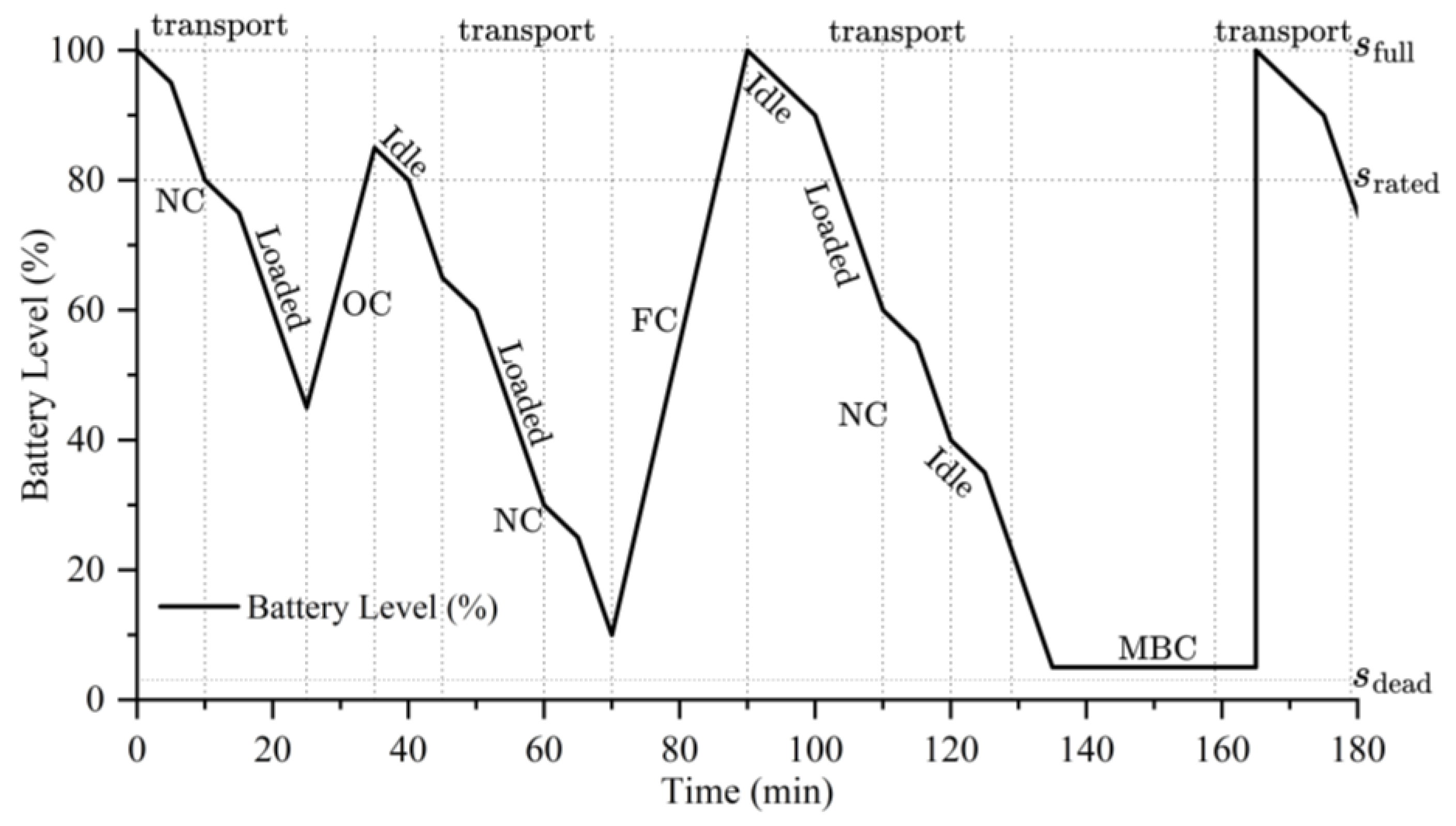
The traditional FJSP with AGVs (FJSP-AGV) is described as follows: In a flexible job shop, there are n jobs to be processed, m machines, and x AGVs. Each job consists of multiple operations, and each operation can be assigned to one machine selected from a set of eligible machines. The processing time for each operation is known and deterministic, and every operation can be processed by at least one machine. Initially, all jobs and AGVs are located at the loading/unloading (L/U) station. AGVs operate in three states: idle, unloaded running, and loaded running. For the first operation of a job, the AGV transports the job from the L/U station to the assigned machine in the loaded state. For subsequent operations, the AGV first travels in the unloaded state to the machine where the job was last processed, and then transports the job in the loaded state to the next assigned machine. Building upon this, this study incorporates AGV charging constraints into the problem formulation, resulting in the FJSPLSP-LTCC model. Specifically, the workshop is equipped with y AGV charger. AGVs, when in the unloaded state, may choose to proceed to a charger for battery replenishment. If the charger is occupied, the AGV must wait until it becomes available. To better reflect practical manufacturing scenarios, three types of AGV charging actions are defined: no charging (NC), opportunity charging (OC), and full charging (FC). OC refers to short-term charging during AGV idle periods to partially replenish battery levels, while FC involves longer charging durations that restore the battery to full capacity. Moreover, to prevent AGV shutdowns due to complete battery depletion, a mandatory maintenance battery change (MBC) policy is introduced, wherein maintenance personnel manually replace the battery for the AGV.

Different strategies are suitable for different practical scenarios: the OC strategy is mainly applied when AGVs have short idle windows; the FC strategy is used when AGVs experience longer idle times or when future tasks are expected to have high energy demands; the MBC strategy serves as an emergency backup, automatically triggered by the system monitoring when AGV battery levels approach depletion. The effects of different charging strategies on AGV battery levels are illustrated in Figure 1. It should be noted that battery degradation effects are not considered in Figure 1; it only reflects the improvements in battery level under different charging strategies.

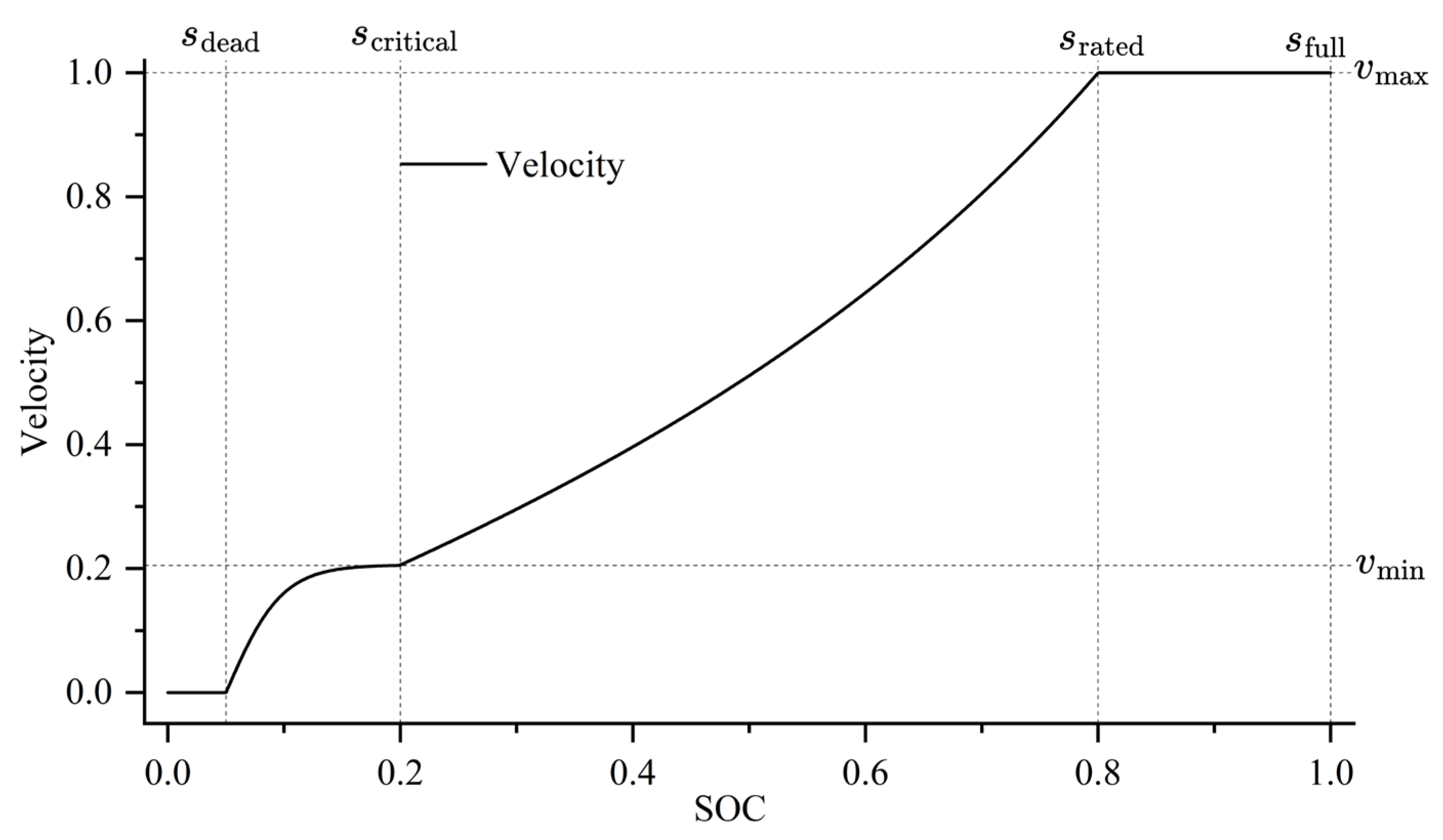
In addition, the FJSPLSP-LTCC model incorporates the battery degradation effect of AGVs, characterized by a nonlinear decline in travel speed as the remaining battery level decreases. This study models the degradation through a four-phase velocity control function, described as follows: Saturation Zone ($s\ge s_{\mathrm{r}\mathrm{a}\mathrm{t}\mathrm{e}\mathrm{d}}$): When energy supply is sufficient, the AGV operates at its rated maximum speed. Decay Zone ($s_{\mathrm{c}\mathrm{r}\mathrm{i}\mathrm{t}\mathrm{i}\mathrm{c}\mathrm{a}\mathrm{l}}<s<s_{\mathrm{r}\mathrm{a}\mathrm{t}\mathrm{e}\mathrm{d}}$): The velocity is determined by a combination of a linear term $\alpha \cdot s$ and an exponential decay term $\beta \cdot e^{-\lambda (s_{\mathrm{r}\mathrm{a}\mathrm{t}\mathrm{e}\mathrm{d}}-s)}$, reflecting the effects of increased internal resistance and polarization that lead to compounded energy losses. Sustainment Zone ($s_{\mathrm{d}\mathrm{e}\mathrm{a}\mathrm{d}}\le s\le s_{\mathrm{c}\mathrm{r}\mathrm{i}\mathrm{t}\mathrm{i}\mathrm{c}\mathrm{a}\mathrm{l}}$): A smooth deceleration trend is modeled using $v_{min}\cdot \mathrm{t}\mathrm{a}\mathrm{n}\mathrm{h}\left({\displaystyle \frac{s-s_{\mathrm{d}\mathrm{e}\mathrm{a}\mathrm{d}}}{s_{\mathrm{c}\mathrm{r}\mathrm{i}\mathrm{t}\mathrm{i}\mathrm{c}\mathrm{a}\mathrm{l}}-s_{\mathrm{d}\mathrm{e}\mathrm{a}\mathrm{d}}}}\cdot \pi \right)$. Failure Zone ($s<s_{\mathrm{d}\mathrm{e}\mathrm{a}\mathrm{d}})$: A deep discharge protection mechanism is triggered, forcing the AGV to shut down in order to prevent battery damage. The corresponding mathematical formulation is given in Equation (1), and the velocity profile under different battery levels is illustrated in Figure 2. Here, $\alpha$ = 0.5, $\beta$ = 0.8, $\lambda$ = 2.5.

$$v(s)=\left\{\begin{array}{ll}1& s\ge s_{\mathrm{r}\mathrm{a}\mathrm{t}\mathrm{e}\mathrm{d}}\\ \alpha \cdot s+\beta \cdot e^{-\lambda (s_{\mathrm{r}\mathrm{a}\mathrm{t}\mathrm{e}\mathrm{d}}-s)}& s_{\mathrm{c}\mathrm{r}\mathrm{i}\mathrm{t}\mathrm{i}\mathrm{c}\mathrm{a}\mathrm{l}}<s<s_{\mathrm{r}\mathrm{a}\mathrm{t}\mathrm{e}\mathrm{d}}\\ v_{min}\cdot tanh\left({\displaystyle \frac{s-s_{\mathrm{d}\mathrm{e}\mathrm{a}\mathrm{d}}}{s_{\mathrm{c}\mathrm{r}\mathrm{i}\mathrm{t}\mathrm{i}\mathrm{c}\mathrm{a}\mathrm{l}}-s_{\mathrm{d}\mathrm{e}\mathrm{a}\mathrm{d}}}}\cdot \pi \right)& s_{\mathrm{d}\mathrm{e}\mathrm{a}\mathrm{d}}\le s\le s_{\mathrm{c}\mathrm{r}\mathrm{i}\mathrm{t}\mathrm{i}\mathrm{c}\mathrm{a}\mathrm{l}}\\ 0& s<s_{\mathrm{d}\mathrm{e}\mathrm{a}\mathrm{d}}\hspace{0.25em}\hspace{0.25em}\hspace{0.25em}\hspace{0.25em}\hspace{0.25em}\hspace{0.25em}\hspace{0.25em}\hspace{0.25em}\end{array}\right.$$

(1)

The FJSPLSP-LTCC problem studied in this paper involves several interdependent decision subproblems, including: (1) selecting a processing machine for each operation; (2) determining the processing sequence of operations on each machine; (3) assigning AGV resources to each operation; and (4) scheduling charging actions for each AGV.

To facilitate the modeling of the FJSPLSP-LTCC, the following assumptions are made:

(1)

All jobs, machines, AGVs, and chargers are initially available;

(2)

The sequence of operations within each job is predetermined and must be followed;

(3)

Each operation can only be processed on one machine at a time;

(4)

Each machine and each AGV can process/transport only one job at a time.

(5)

Once an operation (processing, transportation, or charging) starts, it cannot be interrupted until completion;

(6)

AGVs can only travel along predefined paths;

(7)

AGV speed is updated prior to each movement based on the current battery level and remains constant during the trip;

(8)

Jobs do not need to be returned to the L/U station after the final operation;

(9)

AGVs can only be charged prior to transporting jobs; after each transport task, a forced battery swap is evaluated;

(10)

Each charging station can serve only one AGV at a time;

(11)

Machine failures, job insertions, and AGV path conflicts are not considered.

3.2. An Example for FJSPLSP-LTCC

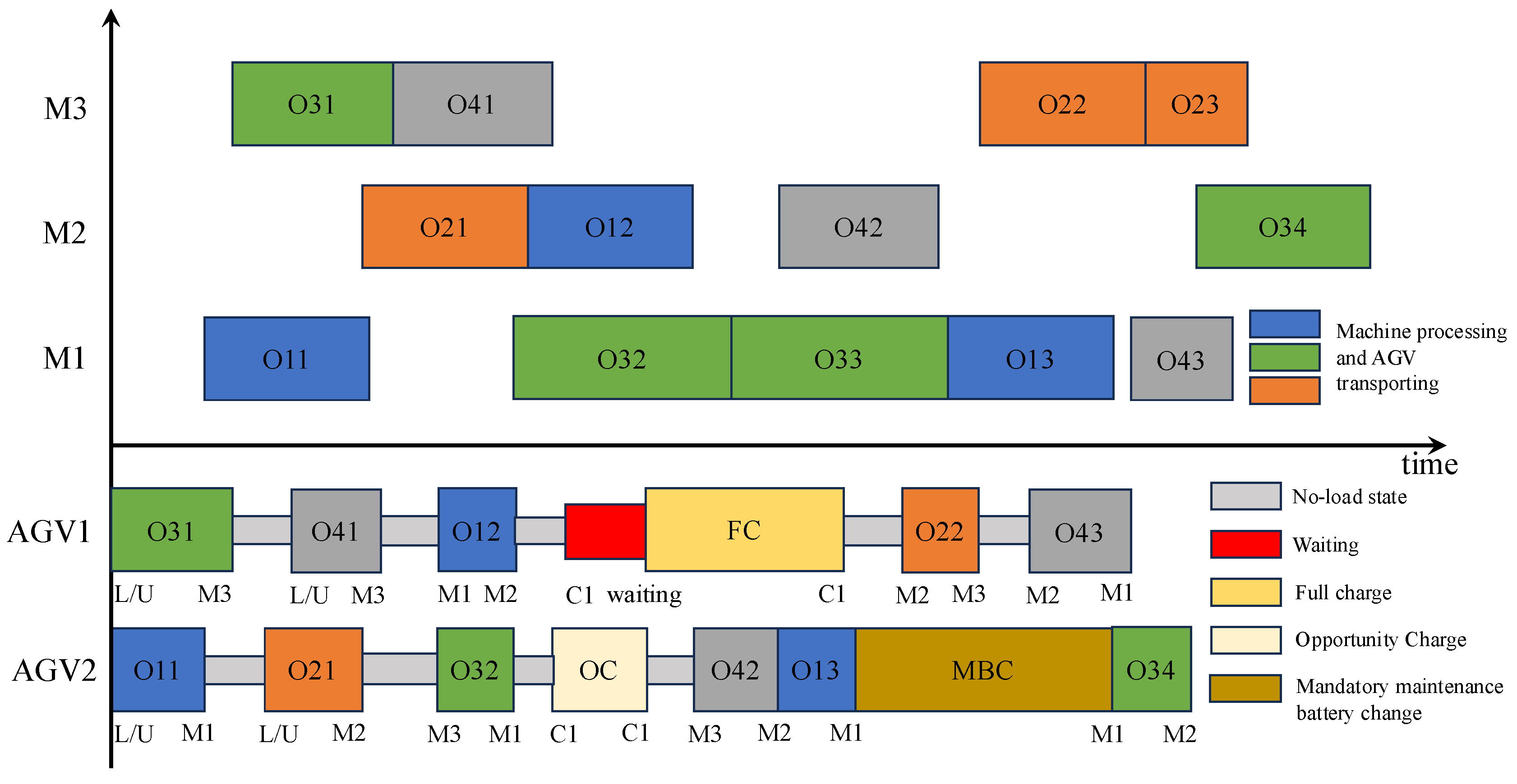
Figure 3 illustrates an instance of the FJSPLSP-LTCC, comprising four jobs, three machines, two AGVs, and one charger. From the AGV perspective, AGV1 initially transports Job 3 from the L/U station to machine M3. Upon completion, it returns to the L/U station in no-load state, picks up Job 4, and transports it to M3. Since M3 is still occupied with Job 3, Job 4 must wait until the machine becomes available before proceeding. Next, AGV1 carries Job 1 from machine M1 to M2. After this transfer, AGV1’s battery level falls below the threshold, selecting an FC operation: it travels to charger C1. However, C1 is occupied by AGV2, so AGV1 remains idle at the charger (highlighted in red in Figure 3) until AGV2 finishes charging. In contrast, after AGV2 transports Job 1 from M2 back to M1, its battery level drops below the maintenance threshold, invoking an MBC procedure. This procedure is performed in situ without relocating the AGV, so AGV2 remains stationary during the process. Finally, note that when consecutive operations of the same job are processed on the same machine—such as Operations 2 and 3 of Job 2 and of Job 3—no AGV transport is required.

3.3. Problem Modeling

Before constructing the mathematical model, it is essential to define the parameters and decision variables used in the formulation.

Table 2. Notations used in FJSPLSP-LTCC.

Notation	Description
Indices
i	Index of job, $i\in J,J=\{\mathrm{1,2},\dots ,J\}$
k	Index of operation, $k\in O_i,O_i=\{\mathrm{1,2},\dots ,K\}$
m	Index of machine, $m\in M,M=\{\mathrm{1,2},\dots ,M\}$
a	Index of AGV, $a\in A,A=\{\mathrm{1,2},\dots ,A\}$
c	Index of Charger, $c\in C,C=\{\mathrm{1,2},\dots ,C\}$
state variables
$C_i$	The completion time of $J_i$
$C_{i,k}$	The completion time of the operation k of job i
$C_{max}$	The maximum completion time of all jobs
$O_i$	Number of operations for the ith job, $i\in J,J=\{\mathrm{1,2},\dots \}$
$M_{i,k}$	The set of machines available for opearation k of job i
$p_{i,k,m}$	The processing time of opearation k on machine m
$s_a$	The power of AGV a
$v_a$	The current speed of AGV a
${\widehat{v}}_a$	The speed of AGV a after charging
$T_{\mathrm{maintain}}$	The time spent on mandatory maintenance battery change
$T_{\mathrm{charge},a}$	The time spent by AGV a from start to finish of charging
$T_{\mathrm{charge}1}$	The time to Opportunity charge
$T_{\mathrm{charge}2}$	The time to fully charge
$T_{\mathrm{wait}}$	The time spent waiting in queue for charging
$D_{\left(a,c\right)}$	The distance from AGV a to charger c
$D_{(\mathrm{source},\mathrm{dest})}$	The distance from the current machine of the job to the specified machine
$D_{\left(c,\mathrm{source}\right)}$	The distance from the charger c to the current machine of the job
$s_a^{\mathrm{new}}$	The power after the AGVs perform an action
$P_{\mathrm{charge}}$	The charging power of AGV
$P_{\mathrm{empty}}$	The empty transport power of AGV
$P_{\mathrm{load}}$	The load power of AGV
$T_{\mathrm{transport},a}^{\mathrm{empty}}$	The empty transport time of AGV
$T_{\mathrm{transport},a}^{\mathrm{load}}$	The load transport time of AGV
$B_{a_1}$	The start charging time of AGV $a_1$
$C_{a_1}$	The time required for AGV $a_1$ charging
$y_{a_1,a_2}$	1 if AGV $a_1$ is charged before $a_2$, and 0 otherwise
M	A large enough positive number
decision variables
$x_{i,k,m}$	1 if machine m processes the opearation k of job i, and 0 otherwise
$y_{i,k,m}$	1 if opearation k is processed on machine m, and 0 otherwise
$w_{i,k,a}$	1 if the opearation k of job i is transported by AGVa, and 0 otherwise
$z_{i,k,a}$	1 if the AGV a transports the opearation k of job i, and 0 otherwise
$d_a$	Charging decisions for AGV a, $d_a=\{\mathrm{1,2},3\}$
$m_a$	Mandatory maintenance battery change decision for AGVa
$y_{a_1,a_2}$	1 if AGV $a_1$ is charged before AGV $a_2$, and 0 otherwise

lists the notations and decision variables involved in the FJSPLSP-LTCC. The objective of this study is to minimize the makespan (the maximum completion time among all jobs). The objective function is formulated as follows:

$$\mathrm{m}\mathrm{i}\mathrm{n}{C}_{max}=\mathrm{m}\mathrm{i}\mathrm{n}\left(\underset{i\in J}{\mathrm{m}\mathrm{a}\mathrm{x}} C_i\right)$$

(2)

Constraints to be considered include the following modules:

Workpiece processing-related constraints, including

1. Precedence constraint.

$$C_{i,k}\ge C_{i,k-1}+p_{i,k,m},\forall i\in J,k\in O_i,m\in M_{i,k}$$

(3)

2. Uniqueness of processing.

$${\sum }_{i\in J} {\sum }_{k\in O_i} x_{i,k,m}\le 1,\forall m\in M$$

(4)

3. Machine assignment constraint.

$${\sum }_{m\in M_{i,k}} y_{i,k,m}=1,\forall i\in J,k\in O_i$$

(5)

AGV transportation related constraints, including:

4. Transportation constraint: each operation must be transported only once.

$${\sum }_{i\in J} {\sum }_{k\in O_i} w_{i,k,a}\le 1,\forall a\in A$$

(6)

5. AGV assignment constraint.

$${\sum }_{a\in A} z_{i,k,a}=1,\forall i\in J,k\in O_i$$

(7)

6. Complete transportation time constraint: includes transportation, charging, and battery change time.

$$T_{\mathrm{transport},a}=\left\{\begin{array}{ll}{\displaystyle \frac{D_{\left(a,\mathrm{source}\right)}}{v_a}}+{\displaystyle \frac{D_{(\mathrm{source},\mathrm{dest})}}{v_a}},& d_a=0\\ {\displaystyle \frac{D_{\left(a,c\right)}}{v_a}}+T_{\mathrm{charge}1}+{\displaystyle \frac{D_{\left(c,\mathrm{source}\right)}}{{\widehat{v}}_a}}+{\displaystyle \frac{D_{(\mathrm{source},\mathrm{dest})}}{{\widehat{v}}_a}},& d_a=1\\ {\displaystyle \frac{D_{\left(a,c\right)}}{v_a}}+T_{\mathrm{charge}2}+{\displaystyle \frac{D_{\left(c,\mathrm{source}\right)}}{{\widehat{v}}_a}}+{\displaystyle \frac{D_{(\mathrm{source},\mathrm{dest})}}{{\widehat{v}}_a}},& d_a=2\\ {{\displaystyle \frac{D_{\left(a,c\right)}}{v_a}}+{\displaystyle \frac{D_{\left(c,\mathrm{source}\right)}}{v_a}}+{\displaystyle \frac{D_{(\mathrm{source},\mathrm{dest})}}{v_a}}+T}_{\mathrm{maintain}},& m_a=1\end{array}\right.$$

(8)

AGV charging and energy management related constraints, including:

7. Charging decision logic constraint.

$$d_a\in \{\mathrm{0,1},2\},\forall a\in A$$

(9)

8. Mandatory maintenance battery change constraint.

$$m_a=\left\{\begin{array}{ll}1,& s_a\le s_{\mathrm{dead}}\\ 0,& \mathrm{e}\mathrm{l}\mathrm{s}\mathrm{e}\end{array}\right.$$

(10)

9. Charging time linkage constraint: charging actions must be recorded with corresponding time and charger availability.

$$T_{\mathrm{charge},a}=\left\{\begin{array}{ll}0,& d_a=0\\ T_{\mathrm{charge}1}+{\displaystyle \frac{D_{\left(a,c\right)}}{v_a}}+T_{\mathrm{wait}}(if exist),& d_a=1\\ T_{\mathrm{charge}2}+{\displaystyle \frac{D_{(a,c)}}{v_a}}+T_{\mathrm{wait}}(if exist),& d_a=2\end{array}\right.$$

(11)

$$T_{\mathrm{charge}2}={\displaystyle \frac{s_{\mathrm{full}}-s_a}{P_{\mathrm{charge}}}}$$

(12)

10. AGV battery update rule: AGV battery levels are updated based on consumption models.

$$s_a^{\mathrm{new}}=\left\{\begin{array}{ll}{s}_a+T_{\mathrm{charge}1}\cdot P_{\mathrm{charge}},& d_a=1\\ s_{\mathrm{full}},& d_a=2\\ s_{\mathrm{full}},& m_a=1\\ s_a-T_{\mathrm{transport},a}^{\mathrm{empty}}{P}_{\mathrm{empty}}-T_{\mathrm{transport},a}^{\mathrm{load}}{P}_{\mathrm{load}},& d_a=0\end{array}\right.$$

(13)

11. Charger exclusivity constraint: each charger can serve only one AGV at a time.

$$\left\{\begin{array}{l}{B}_{a_2}\ge B_{a_1}+C_{a_1}-M\cdot (1-y_{a_1,a_2}),\\ B_{a_1}\ge B_{a_2}+C_{a_2}-M\cdot y_{a_1,a_2},\end{array}\right.$$

(14)

4. Solving FJSPLSP-LTCC Using DRL

As described in Section 3.1, the FJSPLSP-LTCC problem is a complex scheduling problem characterized by sequential decision making, involving several interdependent subtasks: operation assignment, sequencing, AGV scheduling, and charging decision making. DRL is an effective tool for solving such problems.

To mitigate the inherent combinatorial explosion risk in this multi-stage scheduling problem, this study adopts a structured decision-making process by partitioning the overall action space into staged and hierarchical local subspaces. Specifically, machine allocation, operation sequencing, AGV assignment, and charging decisions are conducted separately within their respective stages, significantly reducing the effective action space at each stage. Additionally, within the PPO algorithm framework, a candidate action sampling strategy is designed to eliminate infeasible or evidently inferior action combinations, thereby enhancing learning efficiency and solution quality.

4.1. MDP Formulation

A Markov Decision Process (MDP) is typically defined by a five-tuple: $<S,\mathcal{A},\mathcal{P},\mathcal{C},\gamma >$, where $S$ is the state space, including machine states, job statuses, and AGV states. $\mathcal{A}$ is the action space, covering job selection, machine assignment, AGV selection, charging decisions, and charging station assignment. $\mathcal{P}$ is the state transition probability, denoting the likelihood of transitioning from state $s_t$ to $s_{t+1}$ upon taking action $a_t$. $\mathcal{C}$ is the immediate reward function, representing the feedback received from the environment based on state-action pairs. $\gamma$ is the discount factor that determines the impact of future rewards on current decision-making. The objective of reinforcement learning is to maximize the expected total discounted reward: $\begin{array}{c}{C}_t^{\gamma }=\sum _{t=0}^{\mathrm{\infty }} {\gamma }^t{c}_t(s_t,a_t)\end{array}$. To evaluate the effectiveness of a given policy $\pi$, the following value functions are defined: State Value Function ($V^{\pi }\left(s\right)=\mathbb{E}\left[C_t^{\gamma }\right|s_t=s;\pi ]$), Action Value Function ($\begin{array}{c}{Q}^{\pi }\left(s,a\right)=\mathbb{E}\left[C_t^{\gamma }\right|s_t=\end{array}s,a_t=\left.a;\pi \right]$), Advantage Function (measuring the benefit of an action over the average, $A^{\pi }(s,a)=\begin{array}{c}\mathbb{E}\left[C_t^{\gamma }\right|s_t=s,a_t=a;\pi ]-\mathbb{E}[C_t^{\gamma }|s_t=s;\pi ]\end{array}$). The formulation above lays the foundation for the DRL-based solver using the PPO algorithm presented in the subsequent section.

4.1.1. State

At each decision step $t$, a total of 13 state features are designed to capture the key aspects of the FJSPLSP-LTCC system, including the statuses of machines, jobs, and AGVs. These features form the state vector $s_t$ observed by the agent. The definitions are as follows:

(1) Average utilization rate of machines, denoted as ${URM}_{ave}\left(t\right)$.

$$UR{M}_{ave}\left(t\right)={\displaystyle \frac{{\sum }_{m=1}^M{URM}_m\left(t\right)}{M}}$$

(15)

where ${URM}_m\left(t\right)$ is the utilization rate of machine m, calculated as the total processing time of all operations on machine $m$ divided by its total running time up to time $t$.

(2) Standard deviation of machine utilization rate, denoted as ${URM}_{std}\left(t\right)$.

$$UR{M}_{std}(t)=\sqrt{{\displaystyle \frac{{\sum }_{m=1}^M\left({URM}_m\right(t)-UR{M}_{ave}(t){)}^2}{m}}}$$

(16)

(3) Average completion rate of jobs, denoted as ${CRJ}_{ave}\left(t\right)$.

$${CRJ}_{ave}\left(t\right)={\displaystyle \frac{{\sum }_{i=1}^J{CRJ}_i\left(t\right)}{I}}$$

(17)

where ${CRJ}_i\left(t\right)$ denotes the completion rate of job $i$, defined as the ratio of completed operations to total operations.

(4) Standard deviation of job completion rate, denoted as ${CRJ}_{std}\left(t\right)$.

$$CR{J}_{std}(t)=\sqrt{{\displaystyle \frac{\sum _{i=1}^J \left({CRJ}_i\right(t)-CR{J}_{ave}(t){)}^2}{J}}}$$

(18)

(5) Average remaining processing time of unfinished jobs, denoted as ${RT}_{ave}\left(t\right)$.

$$R{T}_{ave}(t)={\displaystyle \frac{\sum _{i=1}^J R{T}_i\left(t\right)}{{RJ}_{total}}}$$

(19)

where $R{T}_i(t)$ denotes the remaining processing time of job $i$, and is set to 0 if the job is already completed; ${RJ}_{total}$ is the number of unfinished jobs.

(6) Total number of operations remaining for unfinished jobs, denoted as ${RO}_{total}\left(t\right)$.

$${RO}_{total}\left(t\right)={\sum }_{i=1}^n R{O}_i(t)$$

(20)

where $R{O}_i$ is the number of remaining operations for job $i$.

(7) Average current power level of AGVs, denoted as ${CPA}_{ave}\left(t\right)$.

$${CPA}_{ave}\left(t\right)={\displaystyle \frac{{\sum }_{a=1}^A{CPA}_a\left(t\right)}{A}}$$

(21)

where ${CPA}_a\left(t\right)$ is the current power level of AGV $a$.

(8) Standard deviation of AGVs current power level, denoted as ${CPA}_{std}\left(t\right)$.

$${CPA}_{std}\left(t\right)=\sqrt{{\displaystyle \frac{{\sum }_{a=1}^A({CPA}_k\left(t\right)-{CPA}_{ave}\left(t\right){)}^2}{a}}}$$

(22)

(9) Average utilization rate of AGVs, denoted as $UR{A}_{ave}\left(t\right)$.

$$UR{A}_{ave}\left(t\right)={\displaystyle \frac{{\sum }_{a=1}^A{URA}_a\left(t\right)}{A}}$$

(23)

where ${URA}_a\left(t\right)$ is the utilization rate of AGV $a$, calculated as the total material handling time divided by its running time.

(10) Standard deviation of AGV utilization rate, denoted as $UR{A}_{std}\left(t\right)$.

$$UR{A}_{std}(t)=\sqrt{{\displaystyle \frac{{\sum }_{a=1}^A\left({URA}_z\right(t)-UR{A}_{ave}(t){)}^2}{A}}}$$

(24)

(11) Average number of charges for AGVs, denoted as ${NCA}_{ave}\left(t\right)$.

$${NCA}_{ave}\left(t\right)={\displaystyle \frac{{\sum }_{a=1}^A{NCA}_a\left(t\right)}{A}}$$

(25)

where ${NCA}_a\left(t\right)$ denotes the number of times AGV $a$ has charged up to time $t$.

(12) Standard deviation of AGV charge counts, denoted as ${NCA}_{std}\left(t\right)$.

$${NCA}_{std}\left(t\right)=\sqrt{{\displaystyle \frac{{\sum }_{a=1}^A({NCA}_a\left(t\right)-{NCA}_{ave}\left(t\right){)}^2}{A}}}$$

(26)

(13) Total number of AGVs with power below $s_{\mathrm{rated}}$, denoted as ${TAB}_{total}\left(t\right)$.

$${TAB}_{total}\left(t\right)={\sum }_{a=1}^A {TAB}_a(t)$$

(27)

$${TAB}_a\left(t\right)=\left\{\begin{array}{ll}1,& \mathrm{i}\mathrm{f} s_a\left(t\right)<s_{\mathrm{rated}} \\ 0,& \mathrm{e}\mathrm{l}\mathrm{s}\mathrm{e}\end{array}\right.$$

(28)

The 13 state features designed in this subsection are based on a systematic approach, aiming to comprehensively characterize the dynamic characteristics of the FJSPLSP-LTCC system from both operational status and energy management perspectives. Metrics such as the mean and variance of machine utilization and job completion rates quantify production progress and load distribution, aiding the agent in identifying potential bottlenecks and resource allocation inefficiencies. Indicators including the average remaining processing time and the total number of unfinished operations reflect workload intensity and scheduling complexity, providing a basis for reasonable task prioritization to enhance overall scheduling efficiency. Energy-related features encompass the mean and fluctuation of AGV battery levels, the number of low-battery AGVs, and charging frequency, integrating AGV energy status into the scheduling decision framework to effectively coordinate AGV dispatch and charging actions, thereby reducing downtime risks. The comprehensive construction of these features forms a systematic yet concise state representation, equipping the agent with the necessary information to navigate the large decision space and achieve balanced and efficient scheduling decisions.

4.1.2. Action Design

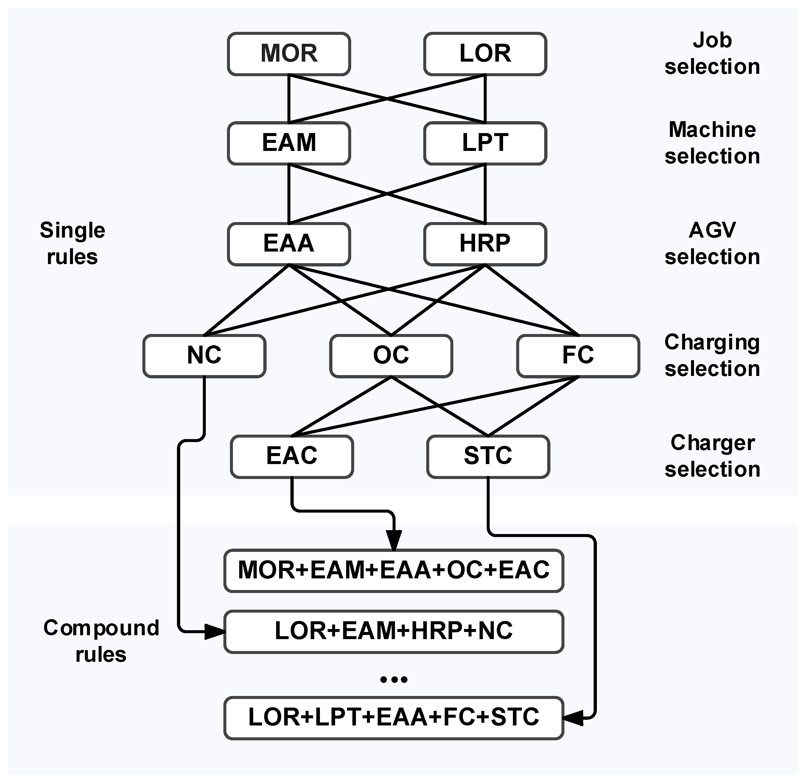
In the proposed FJSPLSP-LTCC model, the agent needs to solve the following sub-problems at each decision point: operation sequencing, machine selection, AGV selection, charging decision, and charger selection. Therefore, each action is essentially a multi-dimensional decision involving the overall scheduling of jobs to resources. To handle this, we design specific action rules at different levels as follows:

• Job selection rules

Two rules are designed for selecting the job: MOR (Most Operations Remaining), which selects the job with the highest number of remaining unprocessed operations. LOR (Least number of Operations Remaining), which selects the job with the fewest remaining operations.

2.

Machine selection rules

Two machine selection strategies are proposed, both based on the set of machines capable of processing the selected operation: EAM (Earliest Available Machine), which selects the machine that becomes available the earliest. LPT (Lowest Processing Time of Machines), which selects the machine with the lowest processing time for the selected operation.

3.

AGV selection rules

Since AGV selection is not constrained by the production process, the following two rules are proposed: EAA (Earliest Available AGV), which selects the AGV that finishes its last transport task earliest. HRP (Highest Remaining Power of AGV), which selects the AGV with the highest remaining battery power.

4.

Charge selections rules

Considering the dynamic battery level of AGVs, three charging options are introduced: NC (Not Charging, no charging is performed). OC (Opportunity Charging), performing opportunity-based partial charging. FC (Full Charge, charging the AGV to full capacity). It should be noted that mandatory maintenance battery change (MBC) is not included in the action space, as it is automatically executed after each transport and is not influenced by state variables.

5.

Charger selections rules

Two rules are proposed for selecting chargers: EAC (Earliest Available Charger) which selects the charger that becomes available first. STC (Shortest Transport Time of Chargers) which selects the charger with the shortest transport time from the current AGV location. Note that if NC is selected, charger selection is not required.

It should be noted that although the proposed action space is constructed through a combination of five hierarchical decision rules, the independence among these rules has been fully considered during the design process. The job selection, machine selection, and AGV selection rules are mutually independent—decisions made in one dimension do not constrain the feasible options in the others. For instance, adopting the MOR or LOR rule for job selection does not restrict the subsequent selection of machines or AGVs. Similarly, the charging decision is designed to remain independent, allowing the agent to autonomously choose among NC, OC, or FC based on the current battery state without relying on prior decision outcomes. To ensure the validity of the action space, the charging station selection rule is activated only when OC or FC is selected. This conditional dependency is explicitly modeled to prevent invalid action combinations. Overall, this structured design guarantees both the validity and expressiveness of the composite action space, facilitating efficient learning while preserving scheduling flexibility. Thus, by combining the decision rules across all five levels above, we construct a set of 40 compound scheduling actions, as shown in Figure 4. Each compound action represents a complete scheduling strategy that spans from job selection to resource allocation and charging operations, forming the action space for reinforcement learning.

4.1.3. Reward

This study adopts minimizing the makespan as the primary scheduling objective. As the goal of reinforcement learning agents is to maximize the expected cumulative reward, the reward function is defined as follows:

$$\begin{array}{c}R(s_t,s_{t+1},a_t)=C_{max}\left(s_t\right)-C_{max}\left(s_{t+1}\right)\end{array}$$

(29)

where $C_{max}\left(s_t\right)$ denotes the maximum completion time of all finished operations at state $s_t$.

The core idea behind this reward design is to encourage the agent to reduce the makespan through each scheduling decision. A decrease in the makespan results in a positive reward, while an increase results in a negative reward. This drives the agent to iteratively improve the scheduling policy toward a globally or near-globally optimal solution.

It is important to note that during the early stages of training, the agent has limited knowledge of the environment, and the reward based on the makespan difference may exhibit high variance due to extensive random exploration, potentially hindering training stability. To mitigate this issue, we employ a reward normalization strategy that dynamically tracks the observed changes in makespan and scales the reward into a bounded range. This normalization facilitates more stable policy updates during the initial training phase. Moreover, the PPO framework inherently includes a clipped surrogate objective and an entropy regularization term, both of which help stabilize learning under high-reward-variance conditions. These mechanisms jointly ensure that the agent can progressively learn effective scheduling behaviors even when starting from a tabula rasa (no prior policy).

4.2. CRGPPO-TKL

This study adopts an enhanced PPO algorithm, named CRGPPO-TKL, to train the collaborative scheduling agent. PPO is a policy gradient method that collects data through interaction with the environment and updates the agent’s policy using stochastic gradient ascent [50]. By employing a clipped surrogate objective and importance sampling, PPO maintains stable policy updates even in high-dimensional combinatorial optimization problems such as machine assignment, AGV selection, charging decisions, and charger selection in the proposed FJSPLSP-LTCC. Unlike value-based methods that only handle discrete action spaces, PPO’s actor-critic architecture allows separate policy heads to process both discrete and continuous actions. As one of the most widely used RL algorithms, PPO has proven its effectiveness in various manufacturing scenarios.

However, PPO still suffers from several limitations. The clipping mechanism, while central to PPO, is sensitive to its clipping range: A narrow clip range may discard many samples due to out-of-range probability ratios (gradient truncation), reducing data efficiency. A wide clip range may lead to policy updates that exceed the trust region, violating the principle of monotonic improvement. To address these issues, Li and Tan [51] proposed Candidate Ratio Guided PPO (CRGPPO), which introduces candidate actions sampled with Gaussian noise. By computing candidate ratios, CRGPPO enables a better assessment of policy divergence and adjusts the clip range adaptively for more stable learning. However, the method is designed for continuous action spaces and introduces randomness that may destabilize training. To address these issues for the discrete decision space of FJSPLSP-LTCC, we propose a modified version called CRGPPO-TKL, with two key enhancements:

• Candidate Action Generation

Since all actions designed in Section 4.1.2 are discrete, we replace the Gaussian noise-based sampling used in CRGPPO with stochastic sampling from the policy’s discrete distribution, making it suitable for the current action space.

$${\pi }_{\theta }\left(a\right|s)=\mathrm{Categorical}(p_1,p_2,\dots ,p_{A_{m\mathrm{a}\mathrm{x}}})$$

(30)

$$a_t^{\left(i\right)}\sim {\pi }_{\theta }(\cdot |s_t)$$

(31)

To balance exploration capability and computational efficiency, we preset the number of candidate actions sampled from the policy distribution to 5 per decision step. This fixed sampling size ensures sufficient coverage of the action space while avoiding excessive computational overhead. Although categorical sampling lacks continuous perturbation mechanisms such as Gaussian noise, the PPO framework incorporates an entropy regularization term to preserve policy stochasticity. This is particularly beneficial in the early training phase, as it promotes diverse action sampling and mitigates the risk of premature convergence to suboptimal policies.

2.

Dynamic Adjustment of the Clipping Range

To reduce training instability, we introduce a target KL divergence mechanism to adjust the clip range dynamically. The update is based on the deviation between the actual KL divergence and the target KL threshold, as follows:

$$r_{\mathrm{action}}={\displaystyle \frac{{\pi }_{\theta }\left(a_t\right|s_t)}{{\pi }_{{\theta }_{\mathrm{o}\mathrm{l}\mathrm{d}}}\left(a_t\right|s_t)}}$$

(32)

$$r_t^{\left(i\right)}(\theta )={\displaystyle \frac{{\pi }_{\theta }\left(a_t^{\left(i\right)}\right|s_t)}{{\pi }_{{\theta }_{\mathrm{o}\mathrm{l}\mathrm{d}}}\left(a_t^{\left(i\right)}\right|s_t)}}$$

(33)

$${\overline{r}}_{\mathrm{candidates}}={\displaystyle \frac{1}{N}}{\sum }_{i=1}^N r_t^{\left(i\right)}(\theta )$$

(34)

$$I_{\mathrm{action}}=\mathbb{I}\left(\left(r_{\mathrm{action}}<1-\epsilon \right)\vee \left(r_{\mathrm{action}}>1+\epsilon \right)\right)$$

(35)

$$I_{\mathrm{candidates}}=\mathbb{I}\left(\left({\overline{r}}_{\mathrm{candidates}}<1-\epsilon \right)\vee \left({\overline{r}}_{\mathrm{candidates}}>1+\epsilon \right)\right)$$

(36)

$${\delta }_{\mathrm{KL}}=\left(I_{\mathrm{action}}+I_{\mathrm{candidates}}\right)/2-T_{\mathrm{KL}}$$

(37)

$${ϵ}_{\mathrm{new}}=\mathrm{clip}({ϵ}_{\mathrm{old}}\cdot \mathrm{e}\mathrm{x}\mathrm{p}(\eta \cdot {\delta }_{\mathrm{KL}}),{ϵ}_{\min },{ϵ}_{\max })$$

(38)

Equations (32) and (33) compute the probability ratios for the current action and sampled candidates, respectively. These ratios quantify how much the policy has changed for a given action after the latest update. Equation (34) computes the average of these ratios across all N sampled candidates. This average serves as a proxy for the policy shift in the local neighborhood of the current action, making the clipping mechanism more robust to action sampling noise.

Equations (35) and (36) generate binary indicators (0 or 1) based on whether the probability ratio of the action or its candidates exceeds the clipping range [$1-\epsilon$, $1+\epsilon$]. Equation (37) computes the deviation ${\delta }_{\mathrm{KL}}$ between the observed clipping violations and $T_{\mathrm{KL}}$. A positive ${\delta }_{\mathrm{KL}}$ suggests excessive policy changes, indicating that the clipping range should be narrowed in the next iteration.

4.3. Training Details

The training process is shown in Figure 5. The notations used and their descriptions are shown in

Table 3. Notations used in CRGPPO-TKL.

Notation	Description
${\pi }_{\theta }\left(a_t\right|s_t)$	Probability distribution of actions output by the current policy network
$a_t^{\left(i\right)}$	i-th candidate action
$A_{m\mathrm{a}\mathrm{x}}$	Maximum number of candidate actions
${\pi }_{{\theta }_{\mathrm{o}\mathrm{l}\mathrm{d}}}$	Old policy network (pre-update policy)
$r_{\mathrm{action}}$	Probability ratio between current and old policies
$r_t^{\left(i\right)}\left(\theta \right)$	Candidate action probability ratio
${\overline{r}}_{\mathrm{candidates}}$	Average probability ratio of candidate actions
$I_{\mathrm{action}}$	Out-of-bound indicator function for action probability ratio
$I_{\mathrm{candidates}}$	Out-of-bound indicator function for candidate average ratio
${\delta }_{\mathrm{KL}}$	KL divergence deviation
${ϵ}_{\mathrm{new}}$	Updated clipping range
${ϵ}_{\min },{ϵ}_{\max }$	Minimum/Maximum clipping range
${\delta }_t$	Temporal Difference (TD) error
$A_t^{GAE}$	Generalized Advantage Estimation (GAE)
$\gamma$	Discount factor
$\lambda$	GAE smoothing coefficient
$\eta$	Adjustment rate
$L^{\mathrm{C}\mathrm{L}\mathrm{I}\mathrm{P}}\left(\theta \right)$	Clipped policy objective
$H\left({\pi }_{\theta }\right)$	Policy entropy

. The specific training steps are as follows:

Step 1: Initialize the actor network parameters $\theta$, the critic network parameters $\varphi$, and the experience replay buffer. Set the initial clipping range $ϵ$, entropy coefficient $\beta$, and target KL divergence threshold $T_{KL}$.

Step 2: Use the current policy ${\pi }_{\theta }$ to interact with the environment and collect transitions in the following form:

$$(s_t,a_t,r_t,s_{t+1})$$

Store these samples in the replay buffer for batch learning.

Step 3: Calculate the advantage estimate using Generalized Advantage Estimation (GAE):

$${\delta }_t=r_t+\gamma V_{\varphi }\left(s_{t+1}\right)-V_{\varphi }\left(s_t\right)$$

(39)

$$A_t^{GAE}={\delta }_t+\left(\gamma \lambda \right){\delta }_{t+1}+\dots$$

(40)

Step 4: For each state $s_t$, generate N candidate actions using the policy ${\pi }_{\theta }$ (Equations (30) and (31)). Compute the average ratio of current to old policy probabilities over the candidates (Equation (34)).

Step 5: Evaluate the current action’s ratio (Equation (32)) to determine whether the current action and candidate ratios exceed the clipping range (Equations (35) and (36)).

Step 6: Calculate the current KL divergence and adjust the clipping range accordingly (Equation (34)).

Step 7: Update the actor by maximizing the clipped surrogate objective with entropy regularization.

$$L^{\mathrm{C}\mathrm{L}\mathrm{I}\mathrm{P}}(\theta )={\mathbb{E}}_t\left[min\left(r_t\left(\theta \right)A_t,\mathrm{c}\mathrm{l}\mathrm{i}\mathrm{p}\left(r_t\right(\theta ),1-ϵ,1+ϵ)A_t\right)\right]$$

(41)

$$L^{\mathrm{A}\mathrm{c}\mathrm{t}\mathrm{o}\mathrm{r}}(\theta )=L^{\mathrm{C}\mathrm{L}\mathrm{I}\mathrm{P}}(\theta )+\beta \cdot {\mathbb{E}}_t\left[H\right({\pi }_{\theta }(\cdot |s_t\left)\right)]$$

(42)

Use gradient ascent to update $\theta$.

Step 8: Update the critic network by minimizing the value loss:

$$L^{\mathrm{V}\mathrm{a}\mathrm{l}\mathrm{u}\mathrm{e}}\left(\varphi \right)={\mathbb{E}}_t\left[{\left(V_{\varphi }\left(s_t\right)-R_t\right)}^2\right]$$

(43)

where $R_t$ is the empirical return. Use gradient descent to update $\varphi$.

Step 9: Repeat Steps 2–8 for multiple iterations until convergence.

The pseudo-code of the CRGPPO-TKL algorithm is shown in Table ‘Algorithm 1’.

Algorithm 1: CRGPPO-TKL training mechanism

Input: Initial actor parameters $\theta$, critic parameters $\varphi$, replay buffer B, clipping range $\epsilon$, entropy coefficient $\beta$, target KL threshold $T_{\mathrm{KL}}$, learning rates ${\alpha }_{\mathrm{a}\mathrm{c}\mathrm{t}\mathrm{o}\mathrm{r}}$, ${\alpha }_{\mathrm{c}\mathrm{r}\mathrm{i}\mathrm{t}\mathrm{i}\mathrm{c}}$, minimum/maximum clipping ${ϵ}_{\mathrm{m}\mathrm{i}\mathrm{n}}$,${ϵ}_{\mathrm{m}\mathrm{a}\mathrm{x}}$, candidate sample size N, clipping update speed$\eta$

1:  while not converged do

2:    Collect trajectories $(s_t,a_t,r_t,s_{t+1})$ using current policy ${\pi }_{\theta }$

3:    Store transitions in replay buffer B

4:    Compute advantages $A_t^{GAE}$ using GAE

5:    for each mini-batch from B do

6:     for each $(s_t,a_t)$ in mini-batch do

7:      Sample N candidate actions $a_t^{\left(i\right)}\sim {\pi }_{\theta }(\cdot |s_t)$

8:      Compute ratio $r_{\mathrm{action}}$ = ${\pi }_{\theta }\left(a_t\right|s_t)$/${\pi }_{{\theta }_{\mathrm{o}\mathrm{l}\mathrm{d}}}\left(a_t\right|s_t)$

9:      Compute ${\overline{r}}_{\mathrm{candidates}}$ = (1/N) ∑${\pi }_{\theta }\left(a_t^{\left(i\right)}\right|s_t)$/${\pi }_{{\theta }_{\mathrm{o}\mathrm{l}\mathrm{d}}}\left(a_t^{\left(i\right)}\right|s_t)$

10:       Compute $I_{\mathrm{action}}$= 1 if $r_{\mathrm{action}}>1+ϵ \mathrm{o}\mathrm{r} r_{\mathrm{action}}<1-ϵ$ else 0

11:       Compute $I_{\mathrm{c}\mathrm{a}\mathrm{n}\mathrm{d}\mathrm{i}\mathrm{d}\mathrm{a}\mathrm{t}\mathrm{e}\mathrm{s}}$= 1 if ${\overline{r}}_{\mathrm{candidates}}>1+ϵ \mathrm{o}\mathrm{r} {\overline{r}}_{\mathrm{candidates}}<1-ϵ$ else 0

12:      end for

13:      Update clipping range:         ${\delta }_{\mathrm{KL}}=\left(I_{\mathrm{action}}+I_{\mathrm{candidates}}\right)/2-T_{\mathrm{KL}}$         ${ϵ}_{\mathrm{new}}=\mathrm{clip}({ϵ}_{\mathrm{old}}\cdot \mathrm{e}\mathrm{x}\mathrm{p}(\eta \cdot {\delta }_{\mathrm{KL}}),{ϵ}_{\min },{ϵ}_{\max })$

14:      Compute policy loss:         $L^{\mathrm{C}\mathrm{L}\mathrm{I}\mathrm{P}}\left(\theta \right)={\mathbb{E}}_t\left[\mathrm{m}\mathrm{i}\mathrm{n}\left(r_t\left(\theta \right)A_t,\mathrm{c}\mathrm{l}\mathrm{i}\mathrm{p}\left(r_t\right(\theta ),1-{ϵ}_{\mathrm{new}},1+{ϵ}_{\mathrm{new}})A_t\right)\right]$         $L^{\mathrm{A}\mathrm{c}\mathrm{t}\mathrm{o}\mathrm{r}}\left(\theta \right)=L^{\mathrm{C}\mathrm{L}\mathrm{I}\mathrm{P}}\left(\theta \right)+\beta \cdot {\mathbb{E}}_t\left[\mathcal{H}\left({\pi }_{\theta }\left(\cdot |s_t\right)\right)\right]$

15:      Update actor: $\theta \leftarrow \theta +{\alpha }_{\mathrm{actor}}{\nabla }_{\theta }{L}_{\mathrm{Actor}}\left(\theta \right)$

16:      Compute value loss: $L^{\mathrm{V}\mathrm{a}\mathrm{l}\mathrm{u}\mathrm{e}}\left(\varphi \right)={\mathbb{E}}_t\left[{\left(V_{\varphi }\left(s_t\right)-R_t\right)}^2\right]$

17:      Update critic: $\varphi \leftarrow \varphi -{\alpha }_{\mathrm{critic}}{\nabla }_{\varphi }{L}_{\mathrm{Value}}\left(\varphi \right)$

18:      $ϵ\leftarrow {ϵ}_{\mathrm{new}}$

19:   end for

20: end while

5. Experiments

In this section, we first utilize the proposed method to determine the optimal number of AGVs under different shop-floor layouts. Then, we compare its performance with compound scheduling rules and other DRL frameworks. Specifically, Section 5.1 describes the benchmark datasets used in the experiments, the layout configurations, and the hyperparameter settings; Section 5.2 applies the proposed CRGPPO-TKL approach to determine the optimal number of AGVs for each layout; Section 5.3 compares the scheduling performance of various methods, assuming the optimal AGV configuration for each layout is fixed.

To compare optimization performance across different methods, we adopt the Optimality Deviation Ratio (ODR), which is calculated as follows:

$$\mathrm{ODR}(s_i)=\left({\displaystyle \frac{s_i-s_{\mathrm{best}}}{s_{\mathrm{best}}}}\right)\times 100\mathrm{\%}$$

(44)

where $s_i$ represents the objective value obtained by algorithm $i$ on a given instance, and $s_{\mathrm{best}}$ is the minimum objective value obtained among all competing methods for that instance. A lower ODR indicates better performance and is closer to the optimal result.

In addition to the ODR metric, this study also employs the independent two-sample t-test to evaluate the statistical significance of performance differences between the proposed CRGPPO-TKL method and baseline approaches, including composite dispatching rules and other DRL-based methods. For each test instance, the ODR values obtained from multiple independent runs are used as input data for the t-test. A significance level of 0.05 is set to determine whether the performance differences are statistically significant.

5.1. Instance Design and Hyperparameter Setting

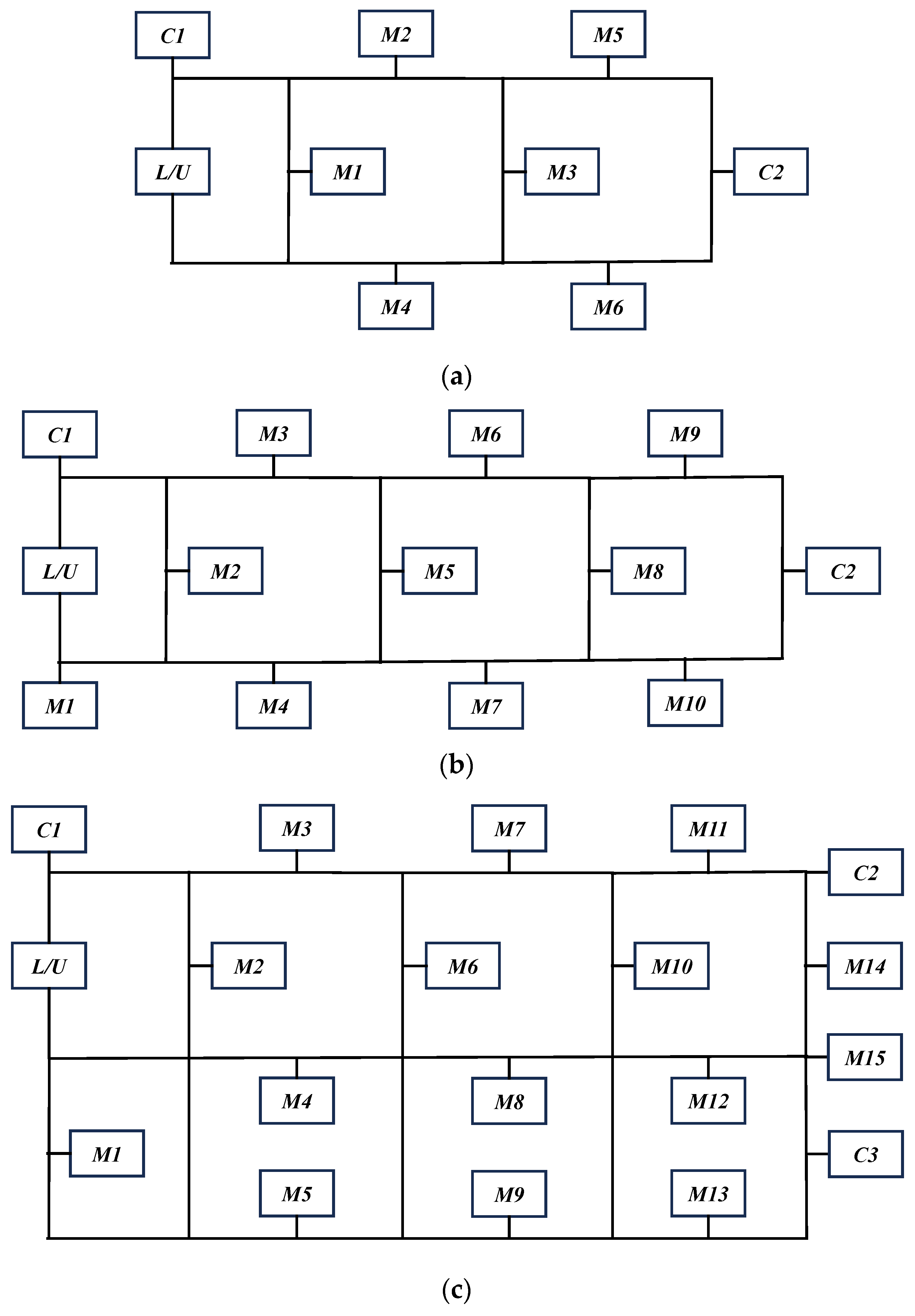
This section utilizes a public benchmark dataset proposed by Brandimarte [2], which includes 10 instances in total (MK01–MK10). To ensure that the proposed method can be evaluated under varying levels of scheduling complexity, this study designs three shop floor layouts by integrating practical manufacturing system scales and benchmark testing considerations. Specifically, the small-scale layout (6 machines) and medium-scale layout (10 machines) reflect typical shop floor sizes found in small to medium-sized manufacturing enterprises, while the large-scale layout (15 machines) is used to simulate more complex large-scale industrial production environments. The ratio of charging stations to machines (approximately one charging station per 5 to 6 machines) is based on commonly observed industrial configurations, aiming to balance AGV availability and mitigate the risk of charging station congestion. Furthermore, the use of varying layout scales facilitates a progressive increase in the decision space of the scheduling problem, thereby enabling a systematic assessment of the proposed scheduling method’s scalability and robustness. These layouts are illustrated in Figure 6, reflecting a progressive increase in shop-floor complexity. Each dataset is assigned to its most suitable layout based on its size and processing requirements, as summarized in

Table 4. Specific information about the dataset.

Benchmarks	Workpiece	Machine	Charger	Layout
MK01–MK02	10	6	2	1
MK03–MK04	15	8	2	2
MK05	15	4	2	1
MK06	10	15	3	3
MK07	20	5	2	1
MK08–MK09	20	10	2	2
MK10	20	15	3	3

. The other parameters used in this paper are set as follows: the initial power of the AGV is a full power of 43,200, the AGV charging power is 1440, the load power is 1200, the no-load power is 600, and the distance between the two locations is equal to the AGV transporting time, and since the FJSP time is dimensionless, the dimensionless data is also used here along with the uniformity of the time scale. For OC, the charging time set in this paper is 10, and for MBC, the time set in this paper is 60.

The proposed algorithm, CRGPPO-TKL, is built on the PPO framework and adopts an Actor-Critic dual-network architecture. The architecture and hyperparameter settings are as follows: The Actor network consists of three fully connected layers that map the input state (including machine status, AGV battery levels, and task queues) to a joint action space. The Tanh activation function is employed to ensure gradient stability, and Softmax is used to generate the policy distribution. The Critic network shares the first two layers of the Actor and outputs the value estimate of the current state.

The parameter settings in this study are based on a combination of established practices in the PPO literature and empirical tuning results specific to the FJSPLSP-LTCC problem. The discount factor $\gamma$, GAE coefficient ${\lambda }_{\mathrm{GAE}}$, entropy regularization coefficient ${\beta }_{\mathrm{entropy}}$, and learning rates ${\eta }_{\mathrm{actor}}$ and ${\eta }_{\mathrm{critic}}$ are selected according to commonly adopted configurations in prior PPO studies [52]. For the newly introduced parameters in the proposed CRGPPO-TKL algorithm—such as the number of candidate actions $N_{\mathrm{candidates}}$, the target KL divergence threshold $T_{\mathrm{KL}}^{\mathrm{target}}$, and the clipping range parameters ${ϵ}_{\mathrm{m}\mathrm{i}\mathrm{n}}/{ϵ}_{\mathrm{m}\mathrm{a}\mathrm{x}}$, and the initial clipping value ${ϵ}_{\mathrm{clip}}$—the values are determined with reference to related literature [51] and experimental experience, aiming to ensure effective policy optimization while maintaining stable and efficient learning.

Additionally, the minimum batch size $B_{min}$, number of update epochs $K_{\mathrm{epoch}}$, and total training time $T_{\mathrm{train}}$ are set based on trade-off analysis between training efficiency and policy performance during preliminary experiments. The complete hyperparameter settings are summarized in

Table 5. Hyperparameter setting of CRGPPO-TKL.

Symbol	Definition	Value
$\gamma$	discount factor	0.99
${\lambda }_{\mathrm{GAE}}$	GAE coefficient	0.95
${ϵ}_{\mathrm{clip}}$	Policy Shear Threshold	0.2
${ϵ}_{\mathrm{m}\mathrm{i}\mathrm{n}}/{ϵ}_{\mathrm{m}\mathrm{a}\mathrm{x}}$	Shear range	0.1$/$0.3
$T_{\mathrm{KL}}^{\mathrm{target}}$	KL dispersion threshold	0.3
${\alpha }_{\mathrm{adjust}}$	Learning rate adjustment step	0.05
${\beta }_{\mathrm{entropy}}$	Entropy regularization factor	0.01
$N_{\mathrm{candidates}}$	Number of candidate actions	5
$K_{\mathrm{epoch}}$	PPO update rounds	4
$B_{min}$	Minimum Batch Size	128
${\eta }_{\mathrm{actor}}/{\eta }_{\mathrm{critic}}$	E-learning rate	$3\times {10}^{-4}/1\times {10}^{-3}$
$T_{\mathrm{train}}$	Total training time	500

.

The algorithm is implemented in Python 3.9 using the PyCharm 2023 development environment. The experiments are run on a laptop system with an Intel Core™ i5-13500HX processor (2.5 GHz) and 16 GB DDR4 RAM.

5.2. Determination of the Optimal Number of AGVs Under Different Layouts

In the FJSPLSP-LTCC problem, the configuration of transport resources is one of the key factors affecting the overall system performance. There exists a significant correlation between the number of AGVs and the system’s makespan: when the number of AGVs is insufficient, the material transport capacity of the system is limited, which tends to increase the waiting time between operations and thus prolong the overall production cycle. Conversely, an excessive number of AGVs may lead to resource waste, increased idle travel rates, and higher operational costs. Therefore, based on the three workshop layouts proposed in Section 5.1, this section conducts a systematic analysis of the performance of each layout under different AGV configurations using the proposed CRGPPO-TKL algorithm, aiming to determine the optimal transport resource configuration for each layout. Each configuration was subjected to 20 independent experimental runs, and the results are presented in

Table 6. Experimental results for different number of AGVs in each layout.

(a) Experimental results for different number of AGVs in layout 1
	MK01			MK02			MK05			MK07
	mean	std	ODR	mean	std	ODR	mean	std	ODR	mean	std	ODR
AGV = 1	337.6	44.3	460.8%	324.1	31.0	512.7%	565.2	29.9	179.2%	683.3	69.3	252.3%
AGV = 2	139.7	6.0	132.1%	149.8	44.8	183.2%	229.4	6.3	13.3%	294.2	59.0	51.7%
AGV = 3	100.4	22.1	66.8%	99.2	23.1	87.4%	202.4	22.5	0.0%	219.0	11.2	12.9%
AGV = 4	78.5	7.8	30.5%	76.4	18.8	44.4%	206.0	22.9	1.8%	209.3	29.2	7.9%
AGV = 5	66.4	2.7	10.3%	59.2	3.3	11.8%	208.4	14.4	3.0%	194.0	17.9	0.0%
AGV = 6	60.2	1.4	0.0%	52.9	2.4	0.0%	204.5	9.3	1.0%	200.2	14.7	3.2%
(b) Experimental results for different number of AGVs in layout 2
	MK03			MK04			MK08			MK09
	mean	std	ODR	mean	std	ODR	mean	std	ODR	mean	std	ODR
AGV = 2	504.0	18.5	112.0%	251.6	5.9	144.5%	1029.9	16.1	65.2%	954.0	15.9	128.9%
AGV = 3	318.7	26.8	34.0%	173.1	21.5	68.2%	751.6	7.2	20.6%	654.1	6.6	56.9%
AGV = 4	258.2	5.8	8.6%	131.6	2.0	27.8%	657.4	13.1	5.5%	552.9	4.4	32.7%
AGV = 5	243.8	4.9	2.5%	115.6	1.8	12.3%	627.0	7.0	0.6%	462.8	4.3	11.0%
AGV = 6	240.2	4.3	1.0%	107.2	1.3	4.1%	623.4	6.2	0.0%	426.0	3.9	2.2%
AGV = 7	237.8	7.9	0.0%	102.9	1.8	0.0%	630.6	16.7	1.2%	416.8	12.9	0.0%
(c) Experimental results for different number of AGVs in layout 3
	MK06						MK10
	mean		std		ODR		mean		std		ODR
AGV = 3	465.4		21.2		186.2%		732.5		40.2		140.1%
AGV = 4	314.1		24.8		93.1%		569.5		5.0		86.7%
AGV = 5	246.2		49.0		51.4%		485.2		11.0		59.0%
AGV = 6	197.3		8.2		21.3%		380.9		6.3		24.9%
AGV = 7	174.3		5.3		7.2%		324.7		4.6		6.4%
AGV = 8	162.6		6.1		0.0%		305.1		1.6		0.0%

where bold indicates the best performance and Figure 7.

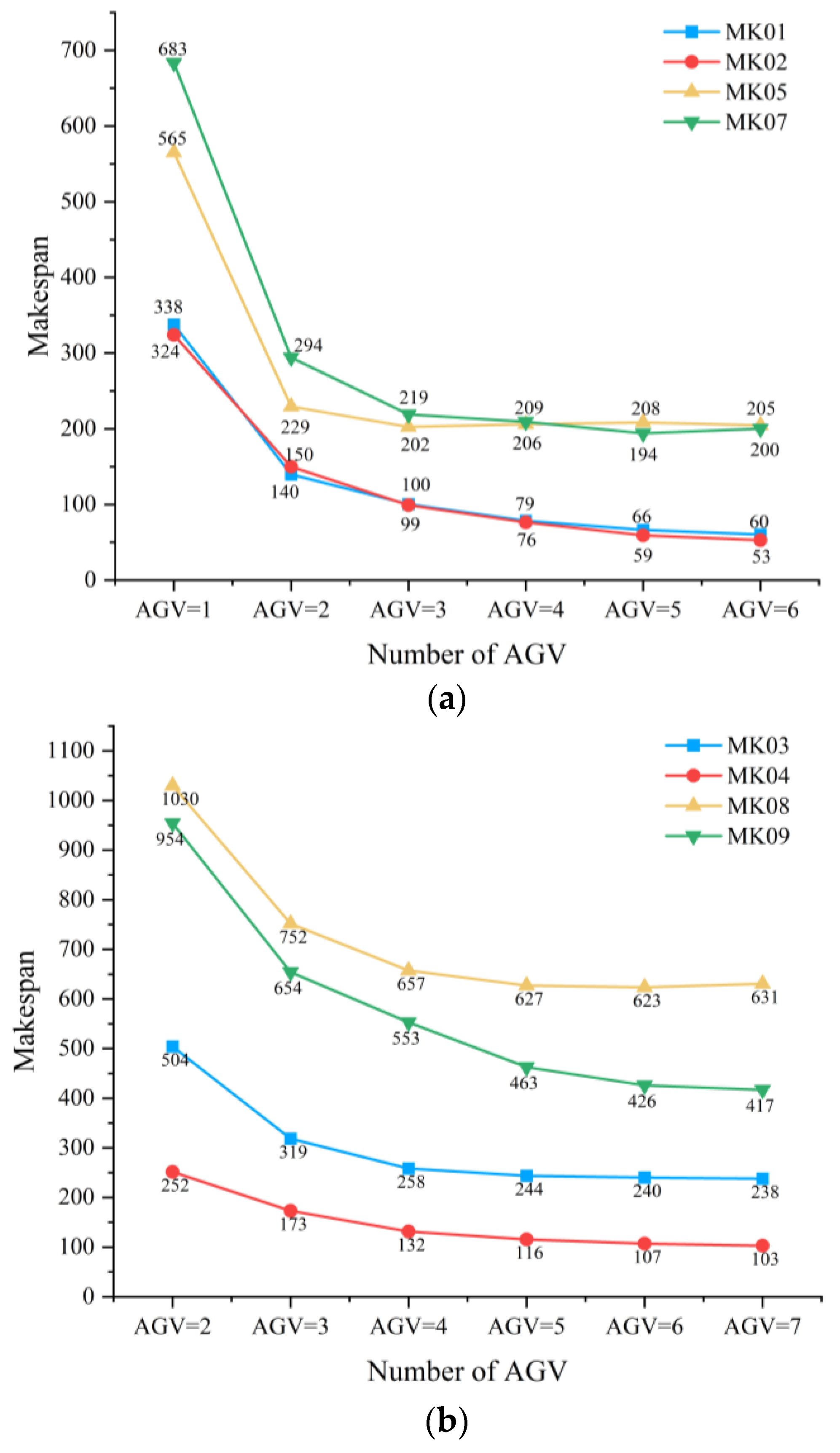
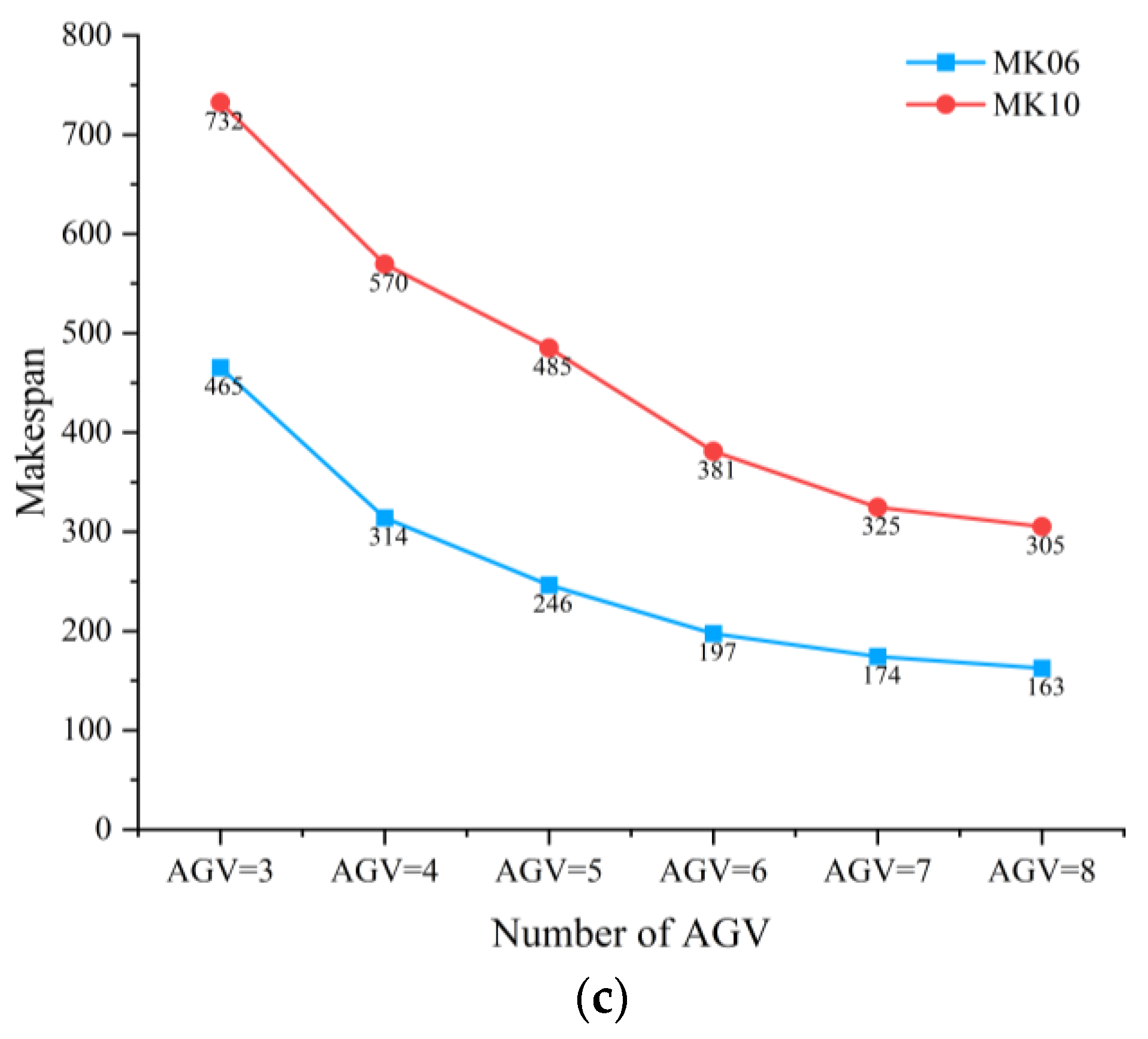
Figure 7 illustrates the significant impact of AGV quantity on the makespan across the three layouts. In Layout 1, when the number of AGVs increases from 1 to 6, the average makespan of test sets MK01, MK02, MK05, and MK07 decreases by 227.4, 271.2, 360.7, and 483.1, corresponding to reductions of 82.2%, 83.7%, 63.8%, and 70.7%, respectively. In Layout 2, when the AGV number increases from 2 to 7, the average makespan of test sets MK03, MK04, MK08, and MK09 decreases by 266.2, 148.7, 399.3, and 537.2, with reduction rates of 52.8%, 59.1%, 38.8%, and 56.3%, respectively. In Layout 3, increasing AGVs from 3 to 8 leads to makespan reductions of 302.8 and 427.4 for MK06 and MK10, corresponding to 65.1% and 58.4%, respectively. Furthermore, it can be observed from Figure 6 that as the number of AGVs increases, the improvement in system makespan gradually diminishes. In some test sets, like MK05 and MK07, the shortest makespan is not achieved with the maximum number of AGVs, indicating that the transport capacity has reached saturation. Therefore, to achieve an optimal balance between transport efficiency and resource cost, it is crucial to determine the optimal AGV quantity for each layout. A detailed analysis of the results for the three layouts is presented below:

In Layout 1, the shortest makespan for test sets MK01, MK02, MK05, and MK07 corresponds to AGV quantities of 6, 6, 3, and 5, respectively. Using these shortest makespans as benchmarks, the ODR for other configurations is calculated, and the same method is applied for Layouts 2 and 3. When the number of AGVs increases from 1 to 2, the ODRs for the respective test sets reach 328.8%, 329.6%, 165.9%, and 200.6%, with an average of 256.2%, indicating that the system efficiency is severely constrained under extreme AGV shortages. As the number of AGVs gradually increases from 2 to 6, the average ODRs decrease to 53.3%, 20.6%, 14.9%, and 5.2%, demonstrating a diminishing marginal benefit. Notably, from Figure 7, it is observed that when AGV quantity exceeds 3, the makespans of MK05 and MK07 tend to stabilize, suggesting that the transport capacity is sufficient for system demands. Therefore, the AGV quantity in Layout 1 is configured as 3 units.

As shown in Figure 7, during the increase in AGV quantity from 4 to 7 in Layout 2, only MK09 exhibits a significant reduction in makespan, while the other three test sets show relatively stable performance. Specifically, when AGVs increase from 4 to 5, the ODR of MK09 is 21.6%, while MK03, MK04, and MK08 have ODRs of only 6.1%, 15.5%, and 4.9%, respectively. Further increasing the number of AGVs from 5 to 7 leads to a further decrease in overall ODR to 4.8%, 1.5%, and even a reverse increase in MK08, indicating that the system has reached its transport saturation. Therefore, the AGV quantity in Layout 2 is configured as 4 units.

In Layout 3, the variation in AGV quantity from 3 to 8 continuously impacts the makespan. The average ODRs for each AGV quantity level are 73.2%, 34.7%, 32.1%, 16.3%, and 6.8%, respectively. Even when AGVs increase from 7 to 8, there is still a 6.8% reduction in makespan, indicating that AGV resources in this layout still contribute to system performance enhancement. However, considering resource utilization efficiency and diminishing marginal returns, to avoid resource waste, the AGV quantity in Layout 3 is configured as 6 units.

5.3. Performance Comparison of CRGPPO-TKL

In this section, we evaluate the effectiveness and generalizability of the proposed CRGPPO-TKL algorithm through comparative experiments conducted under various test scenarios. The comparison includes 40 composite production-logistics scheduling rules designed for the FJSP, two DRL–based scheduling algorithms (including DQN-based and PPO-based methods), as well as a randomized version of CRGPPO-TKL (denoted as RN), in which the agent randomly selects actions at each decision level. Each method was executed over 20 independent runs on each test instance.

5.3.1. Comparison with Composite Scheduling Rules

The 40 composite rules were structured into a two-level hierarchy: the first level involves four machine–job assignment strategies, while the second includes ten AGV charging strategies. The composite actions were indexed sequentially: Actions 1–10 represent the first machine–job pairing combined with each of the ten AGV charging strategies; Actions 11–20 represent the second pairing, and so on. To streamline the analysis, only the best-performing AGV charging strategies under each machine–job rule are presented here; the results of the remaining combinations are provided in Appendix A.

Table 7. Comparison results of selected composite scheduling rules.

	action1		action2		action7		action9		action11		action12		action17		action19		action21		action22		action27		action31		action32		CRGPPO-TKL
	Mean	ODR	Mean	ODR	Mean	ODR	Mean	ODR	Mean	ODR	Mean	ODR	Mean	ODR	Mean	ODR	Mean	ODR	Mean	ODR	Mean	ODR	Mean	ODR	Mean	ODR	Mean	ODR
MK01	106.5	7.5%	105.5	6.5%	231.8	134.0%	259.8	162.2%	110	11.0%	104	5.0%	243.5	145.8%	264.4	166.9%	238.3	140.5%	269.5	172.0%	287.7	190.4%	240	142.2%	258	160.4%	99.1	0.0%
MK02	101.3	8.4%	103.2	10.4%	237.9	154.5%	260.5	178.7%	106	13.4%	112	19.8%	250.8	168.3%	264.7	183.2%	245.9	163.0%	263.2	181.6%	298	218.8%	233	149.2%	239	155.7%	93.5	0.0%
MK03	274.4	5.6%	294.4	13.3%	617.6	137.7%	629.1	142.2%	343	32.0%	343	32.0%	637.6	145.4%	650.8	150.5%	1332.6	413.0%	1460.7	462.3%	1407.8	441.9%	996.8	283.7%	1070.2	312.0%	259.8	0.0%
MK04	143.6	8.9%	143.1	8.6%	380	188.3%	373	183.0%	195	47.9%	195	47.9%	350.3	165.7%	358.7	172.1%	437.6	232.0%	476.2	261.3%	474.6	260.0%	403	205.7%	412	212.5%	131.8	0.0%
MK05	204.7	3.2%	208.7	5.2%	438.9	121.3%	462.6	133.3%	233	17.5%	233	17.5%	440.5	122.1%	472.5	138.3%	645.6	225.5%	680.1	242.9%	694.1	250.0%	701	253.5%	720	263.0%	198.3	0.0%
MK06	208.2	6.4%	215.6	10.2%	538.2	175.1%	502.5	156.9%	216.2	10.5%	221.4	13.2%	600.1	206.8%	562.9	187.7%	906.4	363.3%	1049.4	436.4%	972.5	397.1%	924.3	372.5%	932.8	376.8%	195.6	0.0%
MK07	239.4	9.5%	239.1	9.4%	422.9	93.4%	458	109.5%	239	9.3%	239	9.3%	417.8	91.1%	451.6	106.6%	704.9	222.4%	782.1	257.8%	761.1	248.2%	705.3	222.6%	727.4	232.7%	218.6	0.0%
MK08	675.4	3.3%	764.3	16.9%	979.2	49.8%	1076.4	64.7%	694.7	6.3%	751.5	15.0%	987.5	51.1%	1101	68.5%	3041.7	365.4%	3251.8	397.5%	2918.4	346.5%	2951.3	351.5%	3123.9	378.0%	653.6	0.0%
MK09	579.5	5.0%	716.8	29.9%	1007.6	82.6%	1080.9	95.9%	577.8	4.7%	596.6	8.1%	988.9	79.2%	1045	89.4%	2974.4	439.1%	3215.7	482.8%	2856.8	417.8%	2562	364.3%	2695.1	388.5%	551.8	0.0%
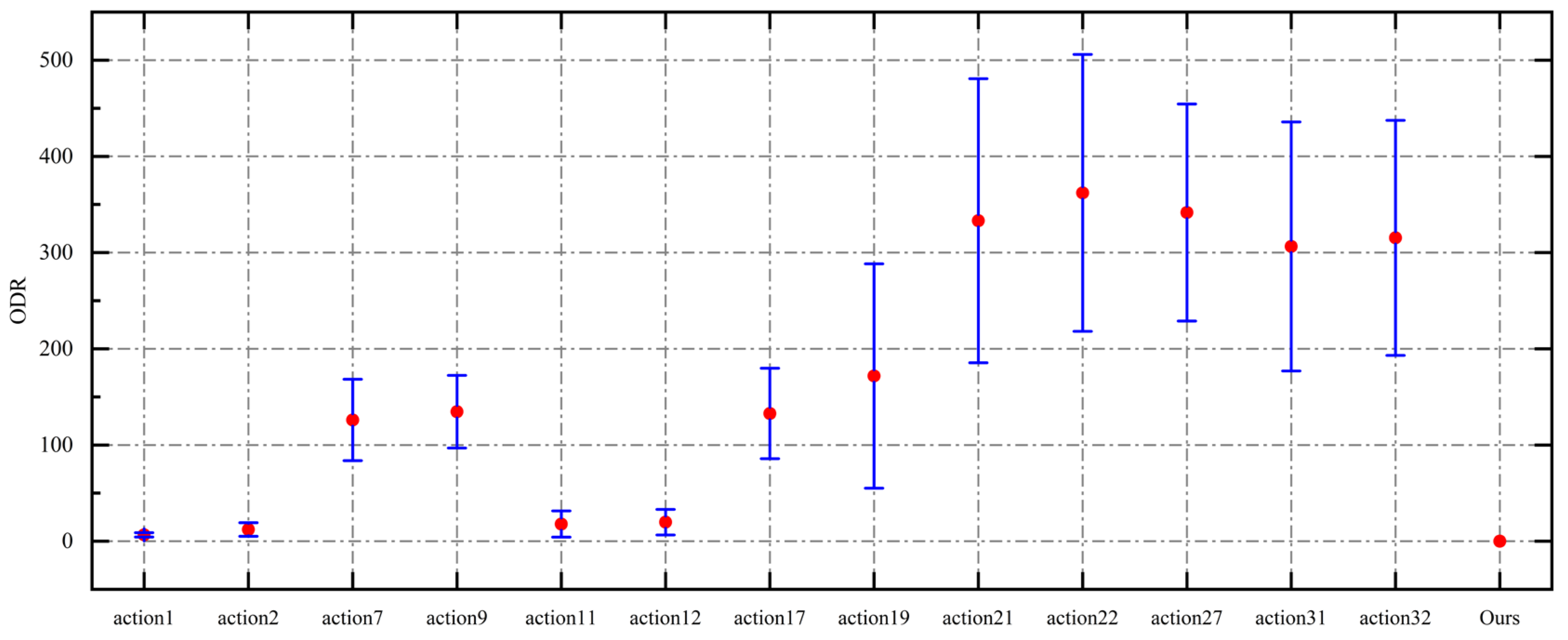
MK10	414.7	8.2%	427.7	11.6%	857.9	123.8%	842	119.7%	483.7	26.2%	499	30.2%	967.2	152.3%	853.4	122.7%	2312.4	503.3%	2670.6	596.8%	2266.7	491.4%	2285.6	496.3%	2410.3	528.9%	383.3	0.0%

summarizes the mean completion times and ODR of CRGPPO-TKL and the selected composite actions across all test instances. Figure 8 visualizes the mean ODR and variance for the selected rules. The results show that CRGPPO-TKL consistently achieved the best completion times across all 10 test instances. The most competitive composite actions were Actions 1, 2, 11, and 12, with average ODRs of 6.6%, 12.2%, 17.9%, and 19.8%, and variances of 2.26, 7.05, 13.64, and 13.28, respectively. Among AGV charging strategies, the 7th and 9th showed superior performance, primarily because the opportunity charging mechanism uses a fixed time duration—AGVs continue charging even if fully charged—while the full-charging strategy terminates once fully charged. As a result, full charging tends to require less time, contributing to shorter completion times. These findings suggest that strategies such as “EAA + STC” and “EAA + EAC”—both of which involve no charging—outperform others, independent of the specific charging policy.

To further validate the performance differences, we conducted independent two-sample t-tests between CRGPPO-TKL and each selected composite scheduling rule across all test instances. The results show that the performance differences are statistically significant (p < 0.05) in all comparisons, confirming that CRGPPO-TKL consistently outperforms composite rule-based methods.

5.3.2. Comparison with Other DRL Algorithms

This subsection evaluates the performance of CRGPPO-TKL against other DRL-based scheduling methods. As shown in

Table 8. Comparison results of other DRLs and RN.

	RN			DQN			PPO			CRGPPO-TKL
	Mean	Std	ODR	Mean	Std	ODR	Mean	Std	ODR	Mean	Std	ODR
MK01	428.1	234.1	332.1%	101.0	2.7	1.9%	101.3	24.0	2.2%	99.1	16.6	0.0%
MK02	516.2	286.2	452.2%	99.8	4.6	6.7%	93.5	20.5	0.05%	93.5	10.7	0.0%
MK03	1674.2	898.7	544.5%	292.4	16.4	12.6%	268.4	24.8	3.3%	259.8	13.7	0.0%
MK04	779.7	430.8	491.5%	142.8	8.9	8.3%	141.7	22.8	7.5%	131.8	1.7	0.0%
MK05	986.3	429.7	397.3%	206.6	2.9	4.2%	198.4	2.6	0.02%	198.3	5.3	0.0%
MK06	1570.6	857.8	717.6%	222.1	9.6	15.6%	192.1	7.1	0.00%	195.6	6.7	1.8%
MK07	870.0	463.0	298.0%	231.0	5.7	5.6%	222.3	35.7	1.67%	218.6	28.8	0.0%
MK08	2951.2	1315.7	351.5%	695.5	18.4	6.4%	758.2	307.2	16.00%	653.6	14.0	0.0%
MK09	2790.6	1327.8	405.8%	601.5	15.5	9.0%	861.0	849.6	56.05%	551.8	6.7	0.0%
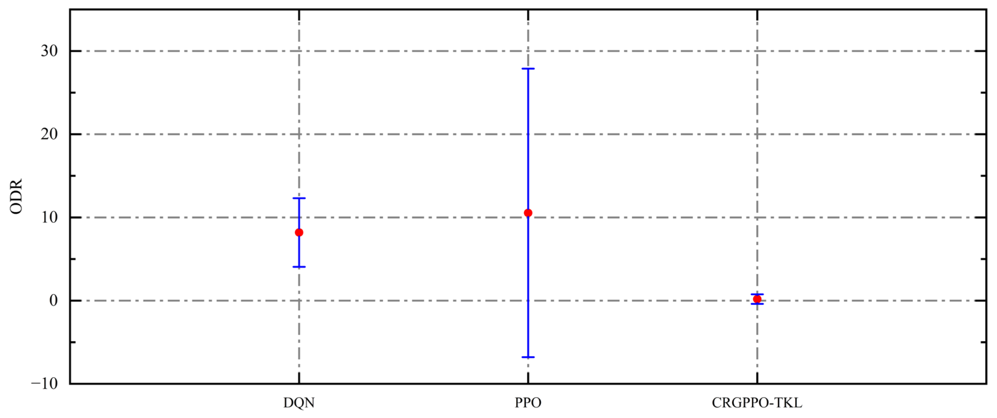
MK10	3163.2	1579.5	725.3%	427.5	16.3	11.5%	454.6	112.6	18.60%	383.3	14.7	0.0%

, CRGPPO-TKL significantly outperforms both the DQN-based and PPO-based methods across 10 MK benchmark instances. It achieves the best performance in 9 out of 10 instances, with MK06 being the only case where PPO slightly outperforms CRGPPO-TKL (ODR = 1.8%). As shown in Figure 9, on average, CRGPPO-TKL achieves an ODR of 0.18%, compared to 8.19% and 10.54% for DQN and PPO, respectively. Furthermore, CRGPPO-TKL exhibits a lower standard deviation of 11.9, in contrast to 10.1 for DQN and a much higher 140.7 for PPO, indicating improved stability alongside superior performance. Notably, PPO exhibits large performance fluctuations on the larger and more complex instances MK08 and MK09, which are characterized by longer completion times. In contrast, CRGPPO-TKL stabilizes performance by dynamically adjusting its clipping range based on the candidate action set, thereby enhancing robustness in complex scenarios. Layout-based statistics (

Table 9. Comparison results of DRL methods under different layouts.

	DQN			PPO			CRGPPO-TKL
	Mean	Std	ODR	Mean	Std	ODR	Mean	Std	ODR
Layout1	159.6	4.0	4.7%	153.9	20.7	1.0%	152.4	15.3	0.0%
Layout2	433.1	14.8	8.5%	507.3	301.1	27.1%	399.2	9.0	0.0%
Layout3	324.8	13.0	12.2%	323.3	59.8	11.7%	289.5	10.7	0.0%

) further reveal that CRGPPO-TKL achieves the lowest average completion time under all three workshop layouts. In contrast, DQN and PPO record average ODRs of 8.5% and 13.3%, and standard deviations of 10.59 and 127.2, respectively. These results underscore the overall performance and robustness of CRGPPO-TKL.

Additionally, independent two-sample t-tests were performed between CRGPPO-TKL and the baseline DRL methods (DQN, PPO) across the 10 MK benchmark instances. The results indicate that the observed improvements of CRGPPO-TKL over DQN and PPO are statistically significant (p < 0.05) in all cases except for MK06, where the difference is not significant. These findings further support the robustness and superior performance of CRGPPO-TKL in complex flexible job shop scheduling scenarios.

5.3.3. Comparison with RN and Action Analysis

As shown in Table 8, CRGPPO-TKL significantly outperforms the random version (RN) in both average completion time and standard deviation. For example, in the MK08 instance, RN records a mean completion time of 2951.2 with a standard deviation of 1315.7, whereas CRGPPO-TKL achieves a mean of 653.6 and a standard deviation of only 14—demonstrating a substantial performance gap. These results confirm that the proposed method does not rely on random action selection but rather learns to make near-optimal decisions at each step, thereby reducing overall system completion time.

To further validate the policy learning capability of CRGPPO-TKL, a detailed action-selection analysis is conducted on MK08, the most challenging instance in terms of average makespan. We conduct 20 independent runs on this instance and record all action selections at each decision point throughout the scheduling process. Actions are then classified and statistically analyzed.

Table 10. Counting by charging action.

Rule	Action Value	Count	Rule	Action Value	Count	Rule	Action Value	Count
NC	1–2	2404	OC	3–6	82	FC	7–10	2
	11–12	1770		13–16	137		17–20	3
	21–22	17		23–26	10		27–30	5
	31–32	39		33–36	29		37–40	2

presents frequency statistics based on charging action types,

Table 11. Counting by machine–job combination action.

Composite Rules	Action Value	Count
MOR + EAM	1–10	2488
MOR + LPT	11–20	1910
LOR + EAM	21–30	32
LOR + LPT	31–40	70

shows results grouped by job–machine combinations, and Figure 10 displays actions that occurred more than 20 times across experiments.

As shown in Table 10, the agent strongly favors the NC action. OC occurs more frequently than FC, while FC actions are rarely chosen. This strategy reflects real-world operational logic: once the optimal number of AGVs is fixed, each vehicle typically performs continuous transport tasks. When battery levels drop, the agent prefers OC during idle gaps, which minimally disrupts production. In contrast, FC often incurs longer delays and is only selected when necessary.

Table 11 indicates that the majority of job–machine combination decisions fall into the MOR + EAM and MOR + LPT categories, accounting for 55.29% and 42.44%, respectively. This suggests that the MOR rule outperforms the LOR in job sequencing, while the EAM heuristic slightly outperforms the LPT rule for machine assignment. Figure 10 shows that, aside from high-frequency non-charging actions like EAA + NC and HRP + NC, the most frequently selected and best-performing actions are EAA + OC + EAC and EAA + OC + STC. This implies that, when minimizing makespan is the sole objective, choosing the EAA and EAM leads to better performance. Meanwhile, EAC and STC perform similarly in charger selection, as both are closely related to completion time. The high frequency of OC further supports earlier conclusions about the efficiency of opportunistic charging.

In summary, CRGPPO-TKL successfully learns to differentiate the effectiveness of different scheduling and charging strategies. It consistently selects actions that accelerate task completion and mitigate resource conflicts and congestion. CRGPPO-TKL not only significantly outperforms the random baseline in overall performance but also demonstrates strong policy learning capabilities and adaptability to complex dynamic environments, confirming its effectiveness and practicality in intelligent industrial scheduling.

5.4. Sensitivity Analysis

To further assess the robustness of the proposed CRGPPO-TKL algorithm with respect to critical hyperparameters and enhance the credibility of our findings, we conducted a sensitivity analysis to evaluate how different parameter settings influence scheduling performance and to validate the rationality of the default configurations.

5.4.1. Experimental Design

The analysis was performed on a medium-scale shop layout (comprising 10 machines and 2 charging stations) using benchmark instances MK03 and MK04 from the MK dataset. Three key hyperparameters were examined: $N_{\mathrm{candidates}}$, $T_{\mathrm{KL}}^{\mathrm{target}}$, and ${ϵ}_{\mathrm{clip}}$. Specifically, $N_{\mathrm{candidates}}$ was tested with values of 3, 5, and 7; $T_{\mathrm{KL}}^{\mathrm{target}}$ with 0.1, 0.2, and 0.3; and ${ϵ}_{\mathrm{clip}}$ with 0.1, 0.2, and 0.3, each with a clipping range of ±0.1. While holding other parameters constant, we systematically varied one parameter at a time and evaluated performance based on the mean Optimality Deviation Rate (ODR), ODR standard deviation, and the number of training epochs required for convergence.

5.4.2. Results and Discussion

The results of the experiment are shown in

Table 12. Parameter sensitivity analysis.

		MK03			MK04
	Value	Mean	Std	ODR	Mean	Std	ODR
Num candidates	3	347.6	42.4	2.6%	193.0	39.7	1.6%
	5	340.2	40.1	0.4%	190.6	33.1	0.4%
	7	338.9	43.9	0.0%	189.9	34.4	0.0%
Target kl	0.1	303.2	32.7	0.0%	156.5	25.0	0.0%
	0.2	333.1	48.8	9.9%	200.5	42.3	28.1%
	0.3	400.4	52.9	32.1%	225.4	38.9	44.0%
Clip epsilon	0.1	442.6	78.9	49.9%	270.5	46.9	80.1%
	0.2	298.8	26.5	1.2%	161.7	43.1	7.7%
	0.3	295.2	29.1	0.0%	150.2	16.2	0.0%

, which indicate that the impact of these hyperparameters on performance varies considerably. The number of candidate actions had minimal influence; ODR and makespan remained relatively stable across different values, suggesting strong robustness under the default setting of $N_{\mathrm{candidates}}$ = 3, 5, 7. In contrast, both $T_{\mathrm{KL}}^{\mathrm{target}}$ and ${ϵ}_{\mathrm{clip}}$ significantly affected performance. Increasing $T_{\mathrm{KL}}^{\mathrm{target}}$ from 0.1 to 0.3 resulted in a substantial rise in ODR—particularly in MK03, where ODR rose from 0% to 32.1%—indicating that an excessively high KL target can destabilize policy updates. Similarly, smaller values of ${ϵ}_{\mathrm{clip}}$ (e.g., 0.1) slowed convergence and introduced greater variability, whereas larger values (e.g., 0.3) yielded better stability and convergence speed.

Based on these findings, we tested a combined setting using the most favorable individual values: $N_{\mathrm{candidates}}=$5, $T_{\mathrm{KL}}^{\mathrm{target}}$ = 0.1, and ${ϵ}_{\mathrm{clip}}$ = 0.3 with a clipping range of [0.2, 0.4]. The results are shown in

Table 13. Comparative analysis results after parameter modification.

	CRGPPO-TKL			CRGPPO-TKL with SA
	Mean	Std	ODR	Mean	Std	ODR
MK01	99.1	16.6	2.8%	96.4	4.8	0.0%
MK02	93.5	10.7	0.7%	92.9	6.0	0.0%
MK03	259.8	13.7	0.0%	260.1	16.8	0.1%
MK04	131.8	1.7	0.1%	131.8	1.4	0.0%
MK05	198.3	5.3	0.7%	197.0	2.2	0.0%
MK06	195.6	6.7	1.1%	193.6	7.0	0.0%
MK07	218.6	28.8	5.3%	207.6	8.4	0.0%
MK08	653.6	14.0	0.0%	656.0	10.0	0.4%
MK09	551.8	6.7	0.0%	555.3	3.8	0.6%
MK10	383.3	14.7	0.0%	394.7	9.4	3.0%

. Compared to the original setting ($T_{\mathrm{KL}}^{\mathrm{target}}$ = 0.3, ${ϵ}_{\mathrm{clip}}$ = 0.2), performance improvements were marginal. For instance, in MK03, ODR slightly increased from 0.0% to 0.1%, while MK04 remained unchanged. This suggests that, although individual parameters may influence performance, the algorithm remains stable under reasonable parameter configurations, demonstrating strong robustness.

5.4.3. Summary

This sensitivity analysis reveals the varying effects of key hyperparameters on convergence and scheduling performance, and confirms the robustness and generalizability of the proposed algorithm under well-tuned settings. These findings provide a solid foundation for future research on adaptive parameter control and large-scale deployment in dynamic production environments.

5.5. Complexity Analysis

To comprehensively evaluate the proposed CRGPPO-TKL algorithm, we analyze its computational and structural complexity, as well as its scalability in practical scheduling scenarios.

5.5.1. Computational Complexity

In each training step, the algorithm samples $N_{\mathrm{candidates}}$ actions from the discrete policy distribution ${\pi }_{\theta }$, computes the probability ratios $r_t^{\left(i\right)}$, evaluates the clipping conditions and adjusts the clipping range based on the estimated KL divergence. Given that these operations are repeated for each state in a mini-batch, the computational complexity per training iteration can be expressed as: $\mathcal{O}(B\cdot N_{\mathrm{candidates}}\cdot F)$, $B$ denotes the batch size and $F$ represents the cost of a single forward/backward pass through the actor-critic network. Although this adds slight overhead compared to standard PPO, the small fixed number of candidates ensures tractability and maintains computational efficiency.

5.5.2. Structural Complexity

The algorithm introduces two enhancements to the standard PPO framework: Candidate action evaluation, which assesses multiple discrete actions before selection, and A dynamic clipping mechanism guided by a target KL divergence.

These modules are implemented independently and plugged into the original PPO structure without altering the core optimization logic. Such modularity improves interpretability, facilitates debugging, and allows for future extension (e.g., adapting to multi-agent or hierarchical settings).

5.5.3. Scalability and Performance Under Different Settings

To assess scalability, we evaluated the algorithm on a range of FJSPLSP-LTCC benchmark instances (MK01–MK10), covering small to large-scale problems with varying machine numbers, transportation resources, and energy constraints. Experimental results confirm that CRGPPO-TKL maintains stable performance and convergence behavior across different problem sizes. This indicates that the proposed method is well-suited for real-world flexible job shop environments with limited transport and energy resources.

5.6. Discussion

The proposed reinforcement learning-based collaborative scheduling method effectively integrates limited transportation resources and AGV charging strategies, addressing challenges such as energy constraints and logistics bottlenecks. Simulation results confirm its ability to reduce makespan, improve scheduling stability, and dynamically adapt to environmental changes. The opportunity charging strategy further enhances AGV utilization under limited transport capacity. Despite its strengths, the method has several limitations, including assumptions of deterministic parameters, simplified battery models, sensitivity to reward design, and the lack of real-world validation. Nonetheless, the approach shows strong potential for smart manufacturing by supporting energy-aware, multi-resource coordination, improving operational efficiency, and offering scalability. Future work will focus on enhancing model realism and deploying the method in digital twin platforms for practical application.

6. Conclusions and Future Research

This paper investigates the production and logistics collaborative scheduling problem in a flexible job shop scheduling environment with limited transport resources and charging constraints. To solve this problem, we introduce CRGPPO-TKL, a novel variant of the PPO algorithm. CRGPPO-TKL samples multiple candidate actions to compute a more comprehensive probability ratio, thereby evaluating policy deviations more thoroughly. Furthermore, it incorporates target scatter KL to dynamically adjust the clipping range, balancing exploration and stability. A 13-dimensional state representation capturing the operational status of machines and AGVs is designed, along with an action space comprising 40 composite scheduling rules. A reward function is formulated to maximize makespan reduction. Using CRGPPO-TKL, the optimal number of AGVs is determined for three facility layouts of different scales. Comparative experiments demonstrate superior learning speed and generalization compared to baseline methods.

Despite these achievements, some limitations remain. The current model assumes deterministic AGV path planning and does not consider path conflicts or dynamic traffic congestion common in high-density shop floors. Additionally, real-world disturbances such as machine breakdowns, order insertions, and stochastic transport delays have not been incorporated into the scheduling framework. Future work will focus on modeling these disturbances and optimizing scheduling accordingly. More accurate nonlinear battery models, including temperature effects, will also be incorporated to improve simulation realism.

Future research will extend the applicability of the proposed method to diverse manufacturing scenarios, such as multi-variety small-batch production and inter-workshop collaboration, enhancing the adaptability and generalization of scheduling algorithms. With the rapid development of Industrial Internet of Things (IIoT) and edge computing, we plan to investigate deploying scheduling strategies on edge devices to enable real-time response and intelligent coordination, providing more efficient and reliable solutions for flexible manufacturing systems.