A Linear Strong Constraint Joint Solution Method Based on Angle Information Enhancement

Abstract

High-precision indoor positioning technology is increasingly prominent in its application value in emerging fields such as the Industrial Internet of Things, smart cities, and autonomous driving. 5G networks can transmit large-bandwidth signals and have the capability to transmit and receive signals with multiple antennas, enabling the simultaneous acquisition of angle and distance observation information, providing a solution for high-precision positioning. Differences in the types and quantities of observation information in complex environments lead to positioning scenarios having a multimodal nature; how to propose an effective observation model that covers multimodal scenarios for high-precision robust positioning is an urgent problem to be solved. This paper proposes a three-stage time–frequency synchronization method based on group peak time sequence tracing. Timing coarse synchronization is performed through a group peak accumulation timing coarse synchronization algorithm for multi-window joint estimation, frequency offset estimation is based on cyclic prefixes, and finally, fine timing synchronization based on the primary synchronization signal (PSS) sliding cross-correlation is used to synchronize 5G signals to chip-level accuracy. Then, a tracking loop is used to track the Positioning Reference Signal (PRS) to within-chip accuracy, obtaining accurate distance information. After obtaining distance and angle information, a high-precision positioning method for multimodal scenarios based on 5G heterogeneous measurement combination is proposed. Using high-precision angle observation values as intermediate variables, this algorithm can still solve a closed-form positioning solution under sparse observation conditions, enabling the positioning system to achieve good positioning performance even with limited redundant observation information.

1. Introduction

The application value of high-precision indoor positioning technology in emerging fields such as the industrial Internet of Things, smart cities, and autonomous driving. Terminal positioning based on 5G mobile communication networks can avoid the construction of large-scale positioning network-dedicated infrastructure, reduce the cost of obtaining high-precision indoor location information, promote the application and promotion of new generation information technology, assist in the construction of a smart society, and promote high-quality economic and social development [1].

The 5G network has greatly increased the types of supported positioning observation information. Integrating this observation information can increase information redundancy, improve positioning accuracy, and enhance positioning reliability, making observation information fusion positioning one of the research hotspots. The support of Multiple-Input Multiple-Output (MIMO) technology for antenna arrays in 5G networks enables base stations to measure the Direction of Arrival (DOA) of uplink signals [2], while the power enhancement of the Ultra Dense Network (UDN) [3] and the Sounding Reference Signal (SRS) enables 5G networks to measure the Time of Arrival (TOA) between terminals and neighboring base stations [4]. Therefore, 5G networks can support various heterogeneous observation information such as the TDOA and the DOA with multiple base stations [5]. Integrating this observation information can compensate for the respective disadvantages of different types of observation information [6], increase information redundancy, improve positioning accuracy, and enhance positioning reliability, making observation information fusion positioning technology one of the research hotspots in the 5G network positioning. 3GPP has also listed observation information fusion positioning as one of the future research directions for 5G networks.

High-precision measurement based on 5G networks requires precise time–frequency synchronization of 5G signals to improve positioning performance. For 5G systems, synchronization to chip accuracy is sufficient to meet communication requirements, but for positioning, precise measurement to chip accuracy is required to obtain more accurate ranging information. 5G high-precision ranging requires time–frequency synchronization first, followed by fine time delay estimation. The accuracy and efficiency of time–frequency synchronization determine the speed of localization convergence. In complex environments, the received signal power may be low, leading to a decrease in synchronization accuracy. Therefore, it is urgent to conduct research on improving synchronization accuracy under low signal-to-noise ratio.

After time–frequency synchronization, the time delay estimation determines the ranging accuracy. Currently, the mainstream time delay estimation methods are divided into super-resolution-based algorithms and correlation discrimination-based algorithms. Super resolution algorithms include high-resolution ranging algorithms based on the Multiple Signal Classification (MUSIC) [7], signal parameter estimation algorithms based on Rotational Invariance Techniques (ESPRIT) [8], and related series of variant algorithms [9].

The algorithm based on correlation discrimination captures and continuously tracks the pilot signal transmitted by the positioning system to obtain time delay and phase measurement values. In traditional capture methods, using cross-correlation (CC) or Matched Filter (MF) methods only achieves a rough estimation of half the symbol width [10,11]. The signal-tracking stage starts from obtaining rough estimates in the acquisition stage and gradually refines the estimation of carrier frequency and code phase parameters through the tracking loop [12,13].

After obtaining 5G distance and angle information, high positioning accuracy can be achieved through fusion positioning at the observation level, which can be divided into filter-based methods and optimization-based methods [14]. Filter-based feature fusion methods use different types of observation information as measurement inputs to the filter, with the terminal position as the system state of the filter. The state is updated through filtering algorithms [15]. Optimization-based feature fusion methods combine various observation information to construct an objective function, solve for the global optimal solution of the objective function, and obtain terminal positioning results [16]. Yifan Zhou et al. used the simulated annealing algorithm for feature fusion positioning calculation of the TDOA and AOA. Through a probabilistic jump mechanism, they avoided local optimal solutions, improved global convergence capability, showed insensitivity to initial values, and enhanced positioning robustness [17]. Javier Díez-González et al. used the genetic algorithm for solving, achieving population iterative optimization through selection, crossover, and mutation operations, promoting extensive search in the solution space [18]. Yi Wang used the particle swarm optimization algorithm to solve feature fusion positioning of the TDOA, TOA, and DOA. By retaining historical optimal solutions and avoiding loss of high-quality solutions, they improved convergence speed while ensuring positioning performance [19].

These heuristic algorithms ensure that positioning results converge to the global optimal solution but incur significant computational time consumption. To improve computational efficiency, K.W. Cheung derived a closed-form solution for distance and angle fusion positioning. By treating the distance from the terminal to the reference base station as a redundant variable, they avoided iterative convergence problems [20]. However, all the above methods perform position calculation by constructing a single observation model. In complex environments, the amount of observation data on line-of-sight paths is limited, redundant observation information is scarce, and scenarios exhibit multimodal characteristics. Each scenario has different types and quantities of observation information, requiring classification and specific modeling for each scenario.

To solve the above problems, this paper makes the following contributions:

(1) A three-stage time–frequency synchronization method based on group peak time sequence tracing is proposed. Timing coarse synchronization is achieved through sliding window group peak identification, frequency offset estimation is performed using cyclic prefixes, and finally, chip-level fine timing synchronization is realized through PSS sliding cross-correlation.

(2) A multimodal positioning algorithm for 5G heterogeneous measurement fusion is proposed: Using high-precision angle observation information as intermediate variables, a linear observation model is constructed for modeling and analysis of multimodal scenarios. Closed-form solution position information is obtained, enabling high-precision robust positioning even when the types and quantities of observations change.

The chapter arrangement of this paper is as follows: Section 2 introduces reference symbols for 5G positioning; Section 3 introduces fine synchronization based on 5G signals and the PRS tracking algorithm to obtain precise distance observations; Section 4 proposes a multimodal positioning algorithm for 5G heterogeneous measurement fusion, constructing a closed-form solution model using high-precision angle observations as intermediate variables to achieve robust positioning under sparse observation conditions; Section 5 conducted experimental simulation verification; Section 6 provides a summary.

2. 5G Reference Signals

5G utilizes various reference signals for distinct functions: the Synchronization Signal Block (SSB) for time–frequency synchronization, the Sounding Reference Signal (SRS) for uplink angle-of-arrival estimation, and the Positioning Reference Signal (PRS) for downlink ranging. We elaborate on these three reference signals in detail.

2.1. The PRS

The 5G downlink positioning reference signal is used to measure the downlink distance of User Equipment (UE), and the generated formula is as follows:

$$\begin{gathered} r\left(m\right)={\displaystyle \frac{1}{\sqrt{2}}}\left(1-2c\left(2m\right)\right)+j{\displaystyle \frac{1}{\sqrt{2}}}\left(1-2c\left(2m+1\right)\right) \\ c(n)=\left(x_1\left(n+N_c\right)+x_2(n+N_c)\right)\mathrm{m}\mathrm{o}\mathrm{d}2 \\ {x}_1\left(n+31\right)=\left(x_1\left(n+3\right)+x_1\left(n\right)\right)\mathrm{m}\mathrm{o}\mathrm{d}2 \\ {x}_2\left(n+31\right)=\left(x_2\left(n+3\right)+x_2\left(n+2\right)+x_2\left(n+1\right)+x_2\left(n\right)\right)\mathrm{m}\mathrm{o}\mathrm{d}2 \end{gathered}$$

(1)

Among them, $N_c=1600$, and the length of the output sequence $c\left(n\right)$, denoted as $M_{PN}$, $n=0,1,\dots ,M_{PN}-1$. The pseudo-random sequences $x_1\left(n\right)$ and $x_2\left(n\right)$ are composed of ${31}^{th}$ order gold codes. The initial value of the first m-sequence $x_1\left(n\right)$ is $x_1\left(0\right)=1,x_1\left(n\right)=0,n=1,2,\dots ,30$. The initial value of the second m-sequence $x_2\left(n\right)$ is:

$$\begin{gathered} c_{init}=\left(2^{22}⌊{\displaystyle \frac{n_{ID,seq}^{PRS}}{1024}}⌋+2^{10}\left(N_{symb}^{slot}{n}_{s,f}^{\mu }+l+1\right)\left(2\left(n_{ID,seq}^{PRS}mod 1024\right)+1\right) \\ +\left(n_{ID,seq}^{PRS}mod 1024\right)\right)mod{2}^{31} \end{gathered}$$

(2)

Among them, $n_{s,f}^{\mu }$ is the time slot number, the downlink PRS sequence ID: $n_{ID,seq}^{PRS}$∈ {0, 1,…, 4095} is given by high-level parameters, and $l$ is the OFDM symbol mapped from the sequence to the time slot.

For each configured downlink PRS resource, the UE assumes that the sequence $r\left(m\right)$ is scaled according to the factor ${\beta }_{PRS}$ and mapped to the resource element ${\left(k,l\right)}_{p,\mu }$, and performs resource mapping according to the following equation:

$$\begin{gathered} a_{k,l}^{\left(p,\mu \right)}={\beta }_{PRS}r(m) \\ m=0,1,\dots \\ k=m{K}_{comb}^{PRS}+\left(\left(k_{offset}^{PRS}+k^{\prime }\right)mod K_{comb}^{PRS}\right) \\ l=l_{start}^{PRS},l_{start}^{PRS}+1,\dots ,l_{start}^{PRS}+L_{PRS}-1 \end{gathered}$$

(3)

Among them, $l_{start}^{PRS}$ is the first symbol of the downlink PRS in the time slot. In the time domain, the size of the downlink PRS resource $L_{PRS}$ ∈ {2,4,6,12}, the comb tooth size $K_{comb}^{PRS}$ ∈ {2,4,6,12}, and the combination of $\left\{L_{PRS,}\right.\left.K_{comb}^{PRS}\right\}$ includes $\left\{2,\right.\left.2\right\}$, $\left\{4,\right.\left.2\right\}$, $\left\{6,\right.\left.2\right\}$, $\left\{12,\right.\left.2\right\}$, $\left\{4,\right.\left.4\right\}$, $\left\{12,\right.\left.4\right\}$, $\left\{6,\right.\left.6\right\}$, $\left\{12,\right.\left.6\right\}$ and $\left\{12,\right.\left.12\right\}$, resource element offset $k_{offset}^{PRS}\in \left\{0,1,\dots ,\right.\left.K_{comb}^{PRS}-1\right\}$.

2.2. The SRS

In 5G uplink positioning, the Sounding Reference Signal (SRS) is used as the positioning signal. The SRS is not a reference signal designed specifically for positioning, but is mainly used to estimate the frequency information of the uplink channel, perform frequency selective scheduling, estimate the uplink channel, etc. At the same time, it can also achieve beamforming scheduling of the base station through the detection of the uplink channel. Due to its autocorrelation and cross-correlation with the positioning reference signal, it is designated as the reference signal for uplink positioning in the 5G Release 16 standard.

The SRS has introduced antenna rotation function in 5G mobile phones, and there are different broadcasting methods on different networks. In non-standalone networks (NSA), 1T1R (1-Transmittor-1-Round) and 1T4R rotation methods are used, while in standalone networks (SA), the 4T4R rotation method is used. The specific rotation method details are as follows:

1T1R, only fixed on one antenna to provide SRS information feedback to the base station, does not support SRS rotation.

1T4R, the terminal alternately transmits SRS signals on four antennas, selecting one antenna to transmit at a time; NSA terminals often use this mode.

2T4R, the terminal alternately transmits SRS signals on four antennas, selecting two antennas to transmit at a time; SA terminals often adopt this mode.

In 5G, the SRS can be configured with [1,2,4] OFDM symbols, which can be consecutive [1,2,4] OFDM symbols located in the last six symbols of a slot. In addition to the periodic SRS and the Aperiodic SRS defined in the LTE SRS, the 5G SRS has added the semi persistent SRS, which has flexibility between periodic and non-periodic SRS.

2.3. The SSB

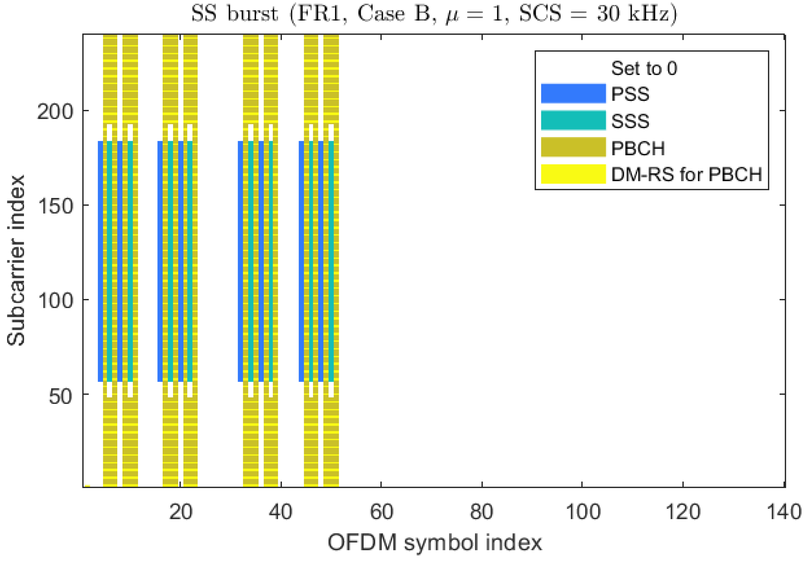
The 5G signal synchronization block (SSB) is used for functions such as cell search, time–frequency synchronization, and beam capture. It consists of a primary synchronization signal (PSS), a secondary synchronization signal (SSS), and a physical broadcast channel (PBCH). The SSB occupies 4 OFDM symbols in the time domain and 240 subcarriers in the frequency domain, corresponding to the numbers {0, 1,…, 239}. The PSS is located on the 127 subcarriers in the middle of the 0th symbol of the SSB, while the SSS is located on the 127 subcarriers in the middle of the 2nd symbol of the SSB, with corresponding subcarrier indices ranging from 56 to 182. The PBCH occupies all 240 subcarriers in the first and third symbols, as well as most subcarriers in the second symbol except for the SSS. The time–frequency resource allocation is shown in the Figure 1.

3GPP selects ZC sequence as the synchronization sequence in LTE, which can achieve good synchronization performance in the 2 GHz frequency band. In 5G NR, as the carrier frequency band increases, larger frequency offsets have a more serious impact on ZC sequences, resulting in a decrease in the peak value of correlation peaks and an increase in false detection rate. To improve the autocorrelation performance and frequency offset resistance of the synchronization sequence, 5G chooses m-sequence as the synchronization sequence to achieve better detection performance when there is a large frequency offset in the initial access.

The PSS and the SSS are orthogonal m-sequences with a length of 127. For all signals transmitted by 5G base stations, there are 3 known possible SSS numbers, corresponding to $N_{ID}^{\left(2\right)}=(0,1,2)$, and 336 known possible SSS numbers, corresponding to $N_{ID}^{\left(1\right)}=\{0,1,\dots 335\}$. Obtain the information of $N_{ID}^{\left(2\right)}$ and $N_{ID}^{\left(1\right)}$ and the frame header position of the received signal by detecting the PSS and the SSS respectively.

The demodulation reference signal (DMRS) is located in the time domain of the first and third symbols of the SSB, and in the frequency domain of the ${(4\mathrm{g}+\mathrm{v})}^{th}$ subcarrier, g = {0, 1,…, 59}. Each symbol is configured with a total of 60 DMRSs, with adjacent DMRSs separated by 4 subcarriers, where v is the starting position of the DMRS, v∈{0, 1, 2, 3}. Determining the uniform arrangement of DMRS in the frequency domain based on the cell number and transmitting antenna sequence number can better reflect the state changes in the signal during transmission.

3. A Synchronization and Fine Ranging Method Based on the 5G Signal

3.1. A Three-Stage Time–Frequency Synchronization Method Based on Group Peak Time Sequence Tracing

When receiving 5G signals, the terminal gradually performs time–frequency synchronization, cell search, and obtains physical broadcast information of the cell based on the SSB. 5G NR introduces a global synchronization grid and a global synchronization channel number (GSCN), and the absolute frequency domain position of the SSB is placed on the global synchronization integer grid. The terminal searches at intervals of the global synchronization grid to obtain the absolute frequency domain position of the SSB. There are six configuration schemes for the time-domain transmission period of the SSB, including 5 ms, 10 ms, 20 ms, 40 ms, 80 ms, and 160 ms. In the actual downlink transmission process, due to the non-transparency of configuration information by users, the terminal assumes a cell search using the SSB with a transmission period of 20 ms after receiving the signal. When the user receives SSB information, they decode the PBCH to obtain the Master Information Block (MIB), perform blind detection using the MIB to obtain the System Information Block (SIB) information, and finally obtain the SSB transmission cycle through the SIB.

Among them, the MIB provides various key physical layer parameters such as system frame number, bandwidth configuration, subcarrier spacing, and PDCCH configuration; the SIB provides detailed system and network information to ensure that terminals complete operations such as access, registration, and reselection. Accurate time–frequency synchronization is crucial for obtaining timely and accurate configuration and network information.

The time–frequency synchronization algorithm is mainly divided into two types: PSS sequence cross-correlation detection and CP-based detection, aiming to obtain the time–frequency information of the PSS and the sector number $N_{ID}^{\left(2\right)}$. The method based on the PSS sequence cross-correlation detection has good resistance to multipath and noise, and can accurately estimate timing information even in low signal-to-noise ratio situations. It can also obtain cell ID information and broadcast information. However, due to the need to match multiple sequences and perform time–frequency scanning separately, this method has high complexity and slow synchronization speed. The method based on CP detection can quickly perform time–frequency synchronization by utilizing the strong correlation between symbol tails and the CP. However, due to the lack of complete data information in the CP, it is unable to obtain cell IDs and broadcast information. In addition, the anti-noise ability of CP-based timing estimation methods is poor. In complex environments, signal attenuation is large and the signal-to-noise ratio of the received signal is low. In this case, using traditional CP-based coarse timing synchronization methods will result in significant errors.

Based on this, this chapter adopts the idea of CP-assisted PSS for fast and robust time–frequency synchronization. To solve the problem of poor coarse timing synchronization performance under low signal-to-noise ratio, this paper proposes a sliding window-based group peak timing coarse synchronization algorithm, which improves the robustness of coarse timing synchronization by jointly estimating the CP in multiple symbols. In complex chemical engineering scenarios, personnel movement is slow and the Doppler effect is not significant. The reason for frequency offset is often due to the phenomenon of frequency asynchrony between the receiving and transmitting ends. Therefore, normalized frequency offset is often a decimal. This article uses a CP-based frequency offset estimation method to estimate and compensate for frequency offset. Afterwards, a method based on sliding PSS cross-correlation was used for fine timing synchronization, ultimately obtaining cell ID information, channel control information, and configuration information of various resources.

In this section, coarse timing estimation is carried out through the group peak timing based on sliding window. Then, frequency offset cancellation is performed based on the CP. Finally, fine time–frequency information synchronization is achieved based on the PSS cross-correlation method. After time–frequency synchronization through the SSB, the SIB can be parsed to obtain relative time–frequency position information of the PRS. Tracking of the PRS is implemented to achieve high-precision distance measurement.

3.1.1. Group Peak Accumulation Timing Coarse Synchronization Algorithms for Multi-Window Joint Estimation

Assuming that the expression of the time-domain baseband signal at the transmitting end is $x\left[n\right]$ and the frequency-domain expression is $X\left[k\right]$; The time-domain expression of the receiver is $y\left[n\right]$, and its corresponding frequency-domain expression is $Y\left[k\right]$. The CP of 5G NR serves as a guard interval and has the same data as the symbol tail, which can effectively perform timing synchronization. Assuming that the number of sampling points for the long CP in OFDM symbols is $N_{CP}$, the number of sampling points for short CP is $N_{cp}$, and the number of sampling points for each symbol is $N_{FFT}$. In the traditional timing coarse synchronization method based on a single sliding window, each sliding window has two sliding windows with a length of $N_{CP}$ sampling points, and the length between the two windows is $(N_{FFT}-N_{CP})$ sampling points. The starting position of a subframe can be estimated by the correlation between the cyclic prefix and the tail of the symbol [21],

$$\widehat{\delta }=\mathrm{a}\mathrm{r}\mathrm{g}\underset{\delta }{max} \left\{\sum _{i=\delta }^{N_{\mathrm{C}\mathrm{P}}-1+\delta } \left|y\left[i\right]y^{\ast }\left[i+N_{FFT}\right]\right|\right\}$$

(4)

Among them, $\widehat{\delta }$ is the time-domain starting position of the subframe obtained through estimation. When the long CP falls exactly into the window, the similarity between the two sliding windows is the highest. When the short CP falls within the sliding window, partial similarity also occurs, but its similarity is smaller than that of the long CP, which can distinguish different symbols in the same subframe.

In simple open spaces, the above method can accurately perform coarse timing synchronization. However, in complex scenarios, signal attenuation is significant and the SNR of the received signal is low, resulting in poor coarse synchronization performance using the above method.

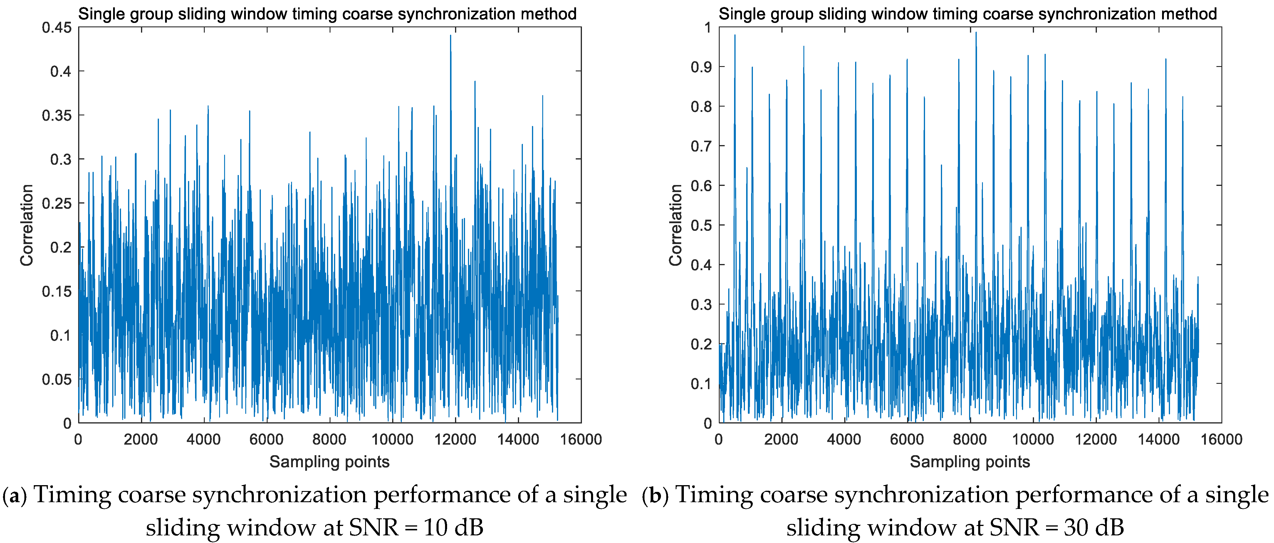
The following Figure 2 compares the timing coarse synchronization performance of a single sliding window under different signal-to-noise ratios, assuming a subcarrier spacing of 30 kHz. When SNR = 30 dB, prominent peaks can be obtained through sliding windows, and the relative position relationship between adjacent peaks is obvious. The first and fifteenth peaks correspond to two long CPs in a subframe, with high correlation. When SNR = 10 dB, the performance of this method deteriorates significantly, and clear peaks cannot be obtained, resulting in a serious decrease in coarse synchronization accuracy.

To enhance the robustness of coarse synchronization, this chapter improves the timing synchronization algorithm of a single sliding window and proposes a group peak accumulation coarse timing synchronization method using a multi-window joint estimation mechanism. In a subframe, the index information $pea{k}_{index}\left(i\right)$ of the group peaks is as follows:

$$pea{k}_{index}(i)=\left\{\begin{array}{cc}1& , i=1\\ 1+N^{\prime }& ,i=2\\ 1+N^{\prime }+(i-2)(N_{FFT}+N_{cp})& ,2<i\le {\displaystyle \frac{n_s}{2}}\\ 1+{\displaystyle \frac{N_{sub}}{2}}& , i={\displaystyle \frac{n_s}{2}}+1\\ 1+{\displaystyle \frac{N_{sub}}{2}}+N^{\prime }& , i={\displaystyle \frac{n_s}{2}}+2\\ 1+{\displaystyle \frac{N_{sub}}{2}}+N^{\prime }+\left(i-{\displaystyle \frac{n_s}{2}}-2\right)(N_{FFT}+N_{cp})& ,{\displaystyle \frac{n_s}{2}}<i\le n_s\end{array}\right.$$

(5)

Among them, $pea{k}_{index}\left(i\right)$ represents the index of the sampling point corresponding to the $i^{th}$ peak in a subframe, $N^{\prime }=N_{FFT}+{\displaystyle \frac{N_{CP}+N_{cp}}{2}}$, $n_s$ is the number of symbols contained in each subframe, and $N_{sub}$ is the number of sampling points in each subframe. The detection function of the long CP can be expressed as:

$$c{p}_{detect}\left(i\right)=\sum _{i=1}^{N_{\mathrm{C}\mathrm{P}}} \left|y\left[i\right]y^{\ast }\left[i+N_{FFT}\right]\right|$$

(6)

The rough timing estimation result obtained by multi-window group peak accumulation based on the CP can be expressed as:

$$\widehat{\delta }=\mathrm{a}\mathrm{r}\mathrm{g}\underset{\delta }{max} \left\{\sum _{i=1}^{n_s} c{p}_{detect}[\delta +pea{k}_{index}(i)-1 ]\right\}$$

(7)

The coarse timing result represents the first subframe of the signal received at the time corresponding to the ${\widehat{\delta }}^{th}$ sample. The first SSB is usually located in the first subframe of the received signal header, and rough timing information of the SSB can be obtained through the relative position relationship of the group peaks.

3.1.2. The Frequency Offset Estimation Method Based on the CP

During the down conversion process of the receiver, phase noise is generated due to the instability of the carrier signal generator, making it difficult for the receiver to generate the exact same carrier frequency as the signal source. If the receiver and the signal source are in relative motion, the relative velocity will produce a Doppler frequency shift. The frequency difference between the transmitter and receiver caused by these two reasons is called the carrier frequency offset (CFO). For the convenience of the following analysis, the CFO will be normalized, namely:

$$\epsilon ={\displaystyle \frac{f_{offset}}{∆f}}={\epsilon }_i+{\epsilon }_f$$

(8)

The impact it has on the receiving end is:

$$y\left[n\right]=x\left[n\right]e^{j2\pi n\epsilon /N_{FFT}}$$

(9)

$$Y\left[k\right]=X[k-\epsilon ]$$

(10)

Among them, ${\epsilon }_i$ is the integer carrier frequency offset (IFO), and ε _f is the fractional carrier frequency offset (FFO). The IFO causes cyclic shift in the signal during reception, but the frequency components of subcarriers still have orthogonality and do not generate intersymbol interference; the FFO will cause distortion in the amplitude and phase of subcarrier components, and as the FFO increases, the amplitude and phase distortions become severe, resulting in inter symbol interference and disrupting the orthogonality between subcarriers.

In complex scenarios, the movement of personnel wearing terminals is slow and does not cause significant Doppler frequency deviation. Fixed normalized frequency deviation is mostly in the form of decimals. Therefore, in this article, only the situation where decimals exist is considered.

After completing the symbol synchronization of the signal, the CFO with a size of $\epsilon$ will cause a phase rotation of $2\pi n\epsilon /N_{FFT}$, resulting in a phase difference of $2\pi \epsilon$ between the symbol tails of the CP and the $N_{FFT}$ sampling points in between. If the CFO does not change in a short period of time, a set of data within a sliding window can be conjugate multiplied and averaged [22]:

$$\widehat{\epsilon }={\displaystyle \frac{1}{2\pi }}\mathrm{a}\mathrm{r}\mathrm{g}\left\{\sum _{n=0}^{N_{\mathrm{c}\mathrm{p}}-1} y[n]y^{\ast }[n+N_{\mathrm{F}\mathrm{F}\mathrm{T}}]\right\}={\displaystyle \frac{1}{2\pi }}\mathrm{a}\mathrm{r}\mathrm{g}\left\{\sum _{n=0}^{N_{\mathrm{c}\mathrm{p}}-1} |x[n]{|}^2{e}^{j2\pi \epsilon }\right\}$$

(11)

Among them, $\mathrm{a}\mathrm{r}\mathrm{g}(\bullet )$ represents the complex number angle taking operation, and the FFO is estimated and compensated by the above method.

3.1.3. The Fine Timing Synchronization Method Based on PSS Sliding Cross-Correlation

After completing coarse timing synchronization, the clock difference between the receiver and transmitter can be regarded as symbol timing offset (STO). When its time-domain length is equal to $\delta$ samples, we can obtain:

$$y\left[n\right]=x[n+\delta ]$$

(12)

$$Y\left[k\right]=e^{j2\pi \delta {\displaystyle \frac{k}{N_{FFT}}}}X[k]$$

(13)

When the STO length is less than one sampling interval, the phase of the received signal will be affected, but it can be restored through channel estimation and channel equalization. When the STO length is greater than one sampling interval, it not only affects the phase, but also causes errors in the starting point position of FFT, resulting in inter symbol interference and inter subcarrier interference. Therefore, it is necessary to estimate the STO to obtain accurate timing information.

After completing the CFO compensation, this chapter conducts fine timing synchronization through the PSS sliding cross-correlation method. After obtaining the coarse timing result $\widehat{\delta }$, the received signal is truncated:

$$\widehat{y}=y\left[n+\widehat{\delta }\right]\epsilon \left[n\right]$$

(14)

Among them, $\epsilon \left[n\right]$ is a step function. The PSS sequence has good correlation in the time domain and good noise resistance in weak signal reception. The following method is used for fine timing estimation:

$$\left\{\begin{array}{c}\widehat{i},\widehat{∆\delta }\end{array}\right\}=\mathrm{a}\mathrm{r}\mathrm{g}\underset{i,∆\delta }{max} \left\{\begin{array}{c}{\displaystyle \frac{{\left|\sum _{n=0}^{N_{FFT}+N_{\mathrm{c}\mathrm{p}}-1}\widehat{y}(∆\delta +n)s_i^{\ast }\left(n\right)\right|}^2}{\sum _{n=0}^{N_{FFT}+N_{\mathrm{c}\mathrm{p}}-1} \widehat{y}(∆\delta +n){\widehat{y}}^{\ast }(∆\delta +n)}}\end{array}\right\}$$

(15)

Among them, $\widehat{∆\delta }$ represents the estimated optimal fine time synchronization error, and $s_i\left(n\right)$ represents the PSS local sequence corresponding to sector $i$, $i\in \{0,1,2\}$. After obtaining fine time synchronization errors, compensation is made for timing information based on coarse timing synchronization to obtain accurate time–frequency information. Afterwards, by performing correlation operations between the received signal and the local PSS and SSS, $N_{ID}^{\left(2\right)}$ and $N_{ID}^{\left(1\right)}$ are obtained, thereby identifying the cell ID information [23]:

$$N_{ID}^{cell}={3N}_{ID}^{\left(1\right)}+N_{ID}^{\left(2\right)}$$

(16)

3.2. Fine Robust Tracking Based on the PRS

In the previous text, a coarse timing estimation method based on sliding windows and a fine timing synchronization method based on the PSS sliding cross-correlation were used for preliminary timing, synchronizing the received signal to the specific sampling points of each time-domain symbol. This is sufficient for communication performance in 5G systems, but for positioning systems, it still has a relatively rough time resolution and cannot obtain accurate ranging information. Since the positioning terminal processes all digital signals, the value between two samples of the transmitted signal can be regarded as the continuous level of the corresponding value of the previous sampling point. For the convenience of expression and not to be confused with the following text, this article refers to it as a chip. To improve time resolution, it is necessary to oversample the received signal by non-integer multiples, so that the sampling points are evenly distributed at different phase positions of the chip, ensuring accurate capture of the chip’s transition time and improving the measurement resolution of the code phase.

To obtain the ranging accuracy within the chip, it is necessary to track the code phase. In this section, a delay phase-locked loop based on lead lag is used for tracking to improve measurement accuracy, while suppressing high-frequency noise in the signal and improving signal-to-noise ratio. The delay phase-locked loop consists of a correlator, a code phase discriminator, a loop filter, and a voltage-controlled oscillator.

After time–frequency synchronization, the received signal has been synchronized to chip accuracy. As the time delay of the 5G signal in the time domain can be equivalent to phase shift in the frequency domain, the locally generated leading and lagging signals in the frequency domain can be represented as:

$$S_{\mathrm{e}\mathrm{a}\mathrm{r}\mathrm{l}\mathrm{y}}\left(k\right)=e^{-j2\pi \xi k/K}S\left(k\right)$$

(17)

$$S_{\mathrm{l}\mathrm{a}\mathrm{t}\mathrm{e}}\left(k\right)=e^{j2\pi \xi k/K}S\left(k\right)$$

(18)

Among them, $k=0,1\dots ,K-1$, $k$ representing the number of subcarrier indices for the PRS; K represents the number of the PRS subcarriers used for positioning; $\xi \in [0.5,1]$ represents the normalized offset in the time domain. By generating local lead and lag sequences, the lead and lag correlations in the frequency domain can be calculated separately [22]

$${\mathcal{R}}_{\mathrm{e}\mathrm{a}\mathrm{r}\mathrm{l}\mathrm{y}}=\sum _{k=0}^{K-1} R^{\prime }(k)S_{\mathrm{e}\mathrm{a}\mathrm{r}\mathrm{l}\mathrm{y}}^{\ast }(k)$$

(19)

$${\mathcal{R}}_{\mathrm{l}\mathrm{a}\mathrm{t}\mathrm{e}}=\sum _{k=0}^{K-1} R^{\prime }(k)S_{\mathrm{l}\mathrm{a}\mathrm{t}\mathrm{e}}^{\ast }(k)$$

(20)

Among them, $R^{\prime }\left(k\right)$ represents the sequence received by the kth subcarrier at the current time. The output of the code phase discriminator can be expressed as:

$$D_{\mathrm{D}\mathrm{L}\mathrm{L}}\triangleq |{\mathcal{R}}_{\mathrm{e}\mathrm{a}\mathrm{r}\mathrm{l}\mathrm{y}}{|}^2-|{\mathcal{R}}_{\mathrm{l}\mathrm{a}\mathrm{t}\mathrm{e}}{|}^2\triangleq K^{2}C{\Lambda }_{\mathrm{D}\mathrm{L}\mathrm{L}}({\tilde{e}}_{\tau },\xi )+N_{\mathrm{D}\mathrm{L}\mathrm{L}}$$

(21)

Among them, $C$ represents the energy of the received signal, and the normalized s-curve ${\Lambda }_{\mathrm{D}\mathrm{L}\mathrm{L}}({\tilde{e}}_{\tau },\xi )$ can be further expressed as:

$${\Lambda }_{\mathrm{D}\mathrm{L}\mathrm{L}}({\tilde{e}}_{\tau },\xi )\triangleq {\left[{\displaystyle \frac{\mathrm{s}\mathrm{i}\mathrm{n}\left(\pi \right({\tilde{e}}_{\tau }-\xi \left)\right)}{K\mathrm{s}\mathrm{i}\mathrm{n}\left(\pi \right({\tilde{e}}_{\tau }-\xi )/K)}}\right]}^2-{\left[{\displaystyle \frac{\mathrm{s}\mathrm{i}\mathrm{n}\left(\pi \right({\tilde{e}}_{\tau }+\xi \left)\right)}{K\mathrm{s}\mathrm{i}\mathrm{n}\left(\pi \right({\tilde{e}}_{\tau }+\xi )/K)}}\right]}^2$$

(22)

Among them, $\xi$ represents the normalized time offset, and the relative relationship between the normalized s-curve and $\xi$ variation is shown in the following Figure 3:

To ensure high tracking sensitivity, the slope at the zero point of the normalized s-curve should be increased, so $\xi =0.5$ was selected in subsequent experiments.

$N_{\mathrm{D}\mathrm{L}\mathrm{L}}$ is represented as code phase discriminator noise, with a mean of zero and variance expressed as:

$$\mathrm{v}\mathrm{a}\mathrm{r}[N_{\mathrm{D}\mathrm{L}\mathrm{L}}]\&\le 2K^2{\sigma }^4\left[1+{\displaystyle \frac{C}{K{\sigma }^2}}{\left({\displaystyle \frac{\mathrm{s}\mathrm{i}\mathrm{n}\left(\pi \right({\tilde{e}}_{\tau }-\xi \left)\right)}{\mathrm{s}\mathrm{i}\mathrm{n}\left(\pi \right({\tilde{e}}_{\tau }-\xi )/K)}}\right)}^2+{\displaystyle \frac{C}{K{\sigma }^2}}{\left({\displaystyle \frac{\mathrm{s}\mathrm{i}\mathrm{n}\left(\pi \right({\tilde{e}}_{\tau }+\xi \left)\right)}{\mathrm{s}\mathrm{i}\mathrm{n}\left(\pi \right({\tilde{e}}_{\tau }+\xi )/K)}}\right)}^2\right]$$

(23)

The discriminator function normalizes based on the characteristic slope at the zero-point error, and then uses a loop filter to achieve zero steady-state error. If the variation in symbol timing error has linear characteristics, a second-order loop filter can be used to achieve zero steady-state error, and its transfer function can be expressed as:

$$F(s)=2\zeta {\omega }_L+{\displaystyle \frac{{\omega }_L^2}{s}}$$

(24)

where ${\omega }_L$ represents the undamped natural frequency of the delay loop, and $\zeta$ represents the damping ratio. To make the step response rise quickly enough, it is usually set to ${\displaystyle \frac{1}{\sqrt{2}}}$, and the noise equivalent bandwidth is set to BL = 0.53${\omega }_L$. The output result of the loop filter is dynamically adjusted through a voltage-controlled oscillator, and the output information of the DLL filter can be represented as $v_{DLL}$. The measured TOA can be updated iteratively using ${\tilde{e}}_{\tau }+{\displaystyle \frac{T_f}{T_s}}{v}_{DLL}$ until convergence.

4. The Joint Positioning Method of Angle and Distance

In complex environments, occlusion has a significant impact on the performance of wireless signal measurement, and it is necessary to identify non-line of sight effects. In this paper, an NLOS recognition method based on comprehensive feature dynamic hierarchical optimization is adopted to effectively identify the propagation state of wireless signals on each path, and finely measure the observations under line-of-sight paths [24]. This article uses an efficient MUSIC algorithm based on fourth-order cumulants for angle search, and performs joint positioning calculation after obtaining angle information [25].

4.1. The Joint Positioning Model of Angle and Distance

To obtain more accurate and robust location information of personnel in chemical plant areas, it is necessary to use downlink ranging and uplink angle measurement information for three-dimensional position estimation. Among them, the terminal coordinates are $\mathit{u}=\left[u_x,u_y,u_z\right]$, the number of base stations is $M$, the coordinates are ${\mathit{s}}_i=\left[x_i,y_i,z_i\right],i=1,2,\dots ,M$. If each base station can transmit ranging signals, that is, the terminal can receive $M-1$ TDOA values, the distance from the terminal to base station $i$ is $d_i$. The TDOA measurement value is:

$$\begin{array}{ccc}{d}_{i,1}=d_i-d_1& =& ‖\mathit{u}-{\mathit{s}}_i‖-‖\mathit{u}-{\mathit{s}}_1‖\\ & =& \sqrt{{\left(x_i-u_x\right)}^2+{\left(y_i-u_y\right)}^2+{\left(z_i-u_z\right)}^2}\\ & -& \sqrt{{\left(x_1-u_x\right)}^2+{\left(y_1-u_y\right)}^2+{\left(z_1-u_z\right)}^2}\end{array}$$

(25)

Among them, $i=2,\dots ,M$. $d_{i,1}$ represents the distance difference between the terminal and the i-th base station and the terminal and the first base station.

But sometimes the hardware conditions of the base station are limited, and angle measurement is sensitive to non-line of sight, resulting in only N sets of effective direction angles ${\theta }_i$ and elevation angles ${\phi }_i$ being obtained, $i=1,2,\dots ,N$. Among them, $N\le M$. This article adopts a method based on comprehensive feature dynamic hierarchical optimization to identify non-line of sight paths, the direction angle and elevation angle are represented as:

$${\theta }_i=\arctan \left({\displaystyle \frac{y_i-u_y}{x_i-u_x}}\right),i=1,2,\dots N$$

(26)

$${\phi }_i=\mathrm{a}\mathrm{r}\mathrm{c}\mathrm{t}\mathrm{a}\mathrm{n}\left({\displaystyle \frac{z_i-u_z}{\left(x_i-u_x\right)cos{\theta }_i+(y_i-u_y)sin{\theta }_i}}\right),i=1,2,\dots N$$

(27)

4.2. A Linear Strong Constraint Joint Solution Method

In the case of good 5G wireless signal coverage performance, there are more base stations with line-of-sight paths, and the corresponding angle and distance observation information is more accurate. In addition, the angle measurement method based on fourth-order cumulants can effectively suppress Gaussian noise and has good noise resistance performance. Based on this, this section assigns higher weight to angle observation information. This not only avoids nonlinear errors caused by constructing observation equations solely based on distance measurement information, but also improves the robustness of the positioning system.

Simultaneously performing tangent calculations on both sides of the direction angle and pitch angle equations, and then shifting the terms, can convert the angle measurement equation into:

$$\left(x_i-u_x\right)sin{\theta }_i-\left(y_i-u_y\right)cos{\theta }_i=0$$

(28)

$$\left(x_i-u_x\right)cos{\theta }_{i}sin{\phi }_i+\left(y_i-u_y\right)sin{\theta }_{i}sin{\phi }_i-\left(z_i-u_z\right)cos{\phi }_i=0$$

(29)

Moving the unknown terminal coordinates to one side of the equation yields

$${sin{\theta }_{i}x}_i-{cos{\theta }_{i}y}_i=sin{\theta }_i{u}_x-{cos{\theta }_{i}u}_y$$

(30)

$$cos{\theta }_{i}sin{\phi }_i{x}_i+sin{\theta }_{i}sin{\phi }_i{y}_i-cos{\phi }_i{z}_i=cos{\theta }_{i}sin{\phi }_i{u}_x+sin{\theta }_{i}sin{\phi }_i{u}_y-cos{\phi }_i{u}_z$$

(31)

Linearize it as

$${\mathit{A}}_1{\mathit{u}}^T={\mathit{h}}_1$$

(32)

$${\mathit{A}}_1=\left[\begin{array}{c}\begin{array}{ccc}sin{\theta }_1& -cos{\theta }_1& 0\\ cos{\theta }_{1}sin{\phi }_1& sin{\theta }_{1}sin{\phi }_1& -cos{\phi }_1\end{array}\\ \dots \\ \begin{array}{ccc}sin{\theta }_N& -cos{\theta }_N& 0\\ cos{\theta }_{N}sin{\phi }_N& sin{\theta }_{N}sin{\phi }_N& -cos{\phi }_N\end{array}\end{array}\right]\in {\mathbb{R}}^{2N\times 3}$$

(33)

$${\mathit{h}}_1=\left[\begin{array}{c}{sin{\theta }_{1}x}_1-{cos{\theta }_{1}y}_1\\ cos{\theta }_{1}sin{\phi }_1{x}_1+sin{\theta }_{1}sin{\phi }_1{y}_1-cos{\phi }_1{z}_1\\ \dots \\ {sin{\theta }_{N}x}_N-{cos{\theta }_{N}y}_N\\ cos{\theta }_{N}sin{\phi }_N{x}_N+sin{\theta }_{N}sin{\phi }_N{y}_N-cos{\phi }_N{z}_N\end{array}\right]\in {\mathbb{R}}^{2N\times 1}$$

(34)

In practical scenarios, due to hardware limitations such as antenna arrays, RF front-end, and baseband processors, not all base stations can accurately measure angles. This section discusses situations where only one channel of accurate angle information can be obtained and situations where multiple channels of accurate angle information can be obtained.

When only one accurate angle observation can be obtained through measurement, its corresponding base station is used as the differential station of the TDOA. The distance difference formula is rewritten as $d_{i,1}+‖\mathit{u}-{\mathit{s}}_1‖=‖\mathit{u}-{\mathit{s}}_i‖$, and the square of both sides is obtained:

$${d_{i,1}}^2+{‖{\mathit{s}}_1‖}^2-{‖{\mathit{s}}_i‖}^2=2\left({\mathit{s}}_1-{\mathit{s}}_i\right){\mathit{u}}^T-2d_{i,1}{d}_1$$

(35)

Among them, $d_1$ and $\mathit{u}$ are unknown variables with correlation. The commonly used methods for solving such functions are two-step weighted least squares and semi definite relaxation algorithms that simultaneously estimate unknown parameters and auxiliary variables. These methods have high complexity. In this section, the relationship between base stations and terminals is constructed by enhancing the weight of angle observation information, it can be obtained that:

$$\mathit{u}-{\mathit{s}}_1=d_1{\mathit{b}}_{\mathbf{1}}$$

(36)

Among them, ${\mathit{b}}_{\mathbf{1}}=[cos{\theta }_{1}cos{\phi }_1,sin{\theta }_{1}cos{\phi }_1,sin{\phi }_1]$, is the unit vector of the terminal relative to the angle measuring base station, that is:

$${d_{i,1}}^2+{‖{\mathit{s}}_1‖}^2-{‖{\mathit{s}}_i‖}^2=2\left({\mathit{s}}_1-{\mathit{s}}_i\right){\mathit{u}}^T-2d_{i,1}{d}_1{\mathit{b}}_{\mathbf{1}}{{\mathit{b}}_{\mathbf{1}}}^{\mathit{T}}$$

(37)

$${d_{i,1}}^2+{‖{\mathit{s}}_1‖}^2-{‖{\mathit{s}}_i‖}^2-2d_{i,1}{\mathit{b}}_{\mathbf{1}}{{\mathit{s}}_1}^T=2\left({\mathit{s}}_1-{\mathit{s}}_i-d_{i,1}{\mathit{b}}_{\mathbf{1}}\right){\mathit{u}}^T$$

(38)

Linearize it as

$${\mathit{A}}_2{\mathit{u}}^T={\mathit{h}}_2$$

(39)

$${\mathit{A}}_2=\left[\begin{array}{c}2\left({\mathit{s}}_1-{\mathit{s}}_2-d_{2,1}{\mathit{b}}_{\mathbf{1}}\right)\\ \dots \\ 2\left({\mathit{s}}_1-{\mathit{s}}_M-d_{M,1}{\mathit{b}}_{\mathbf{1}}\right)\end{array}\right]\in {\mathbb{R}}^{(M-1)\times 3}$$

(40)

$${\mathit{h}}_2=\left[\begin{array}{c}{d_{2,1}}^2+{‖{\mathit{s}}_1‖}^2-{‖{\mathit{s}}_2‖}^2-2d_{2,1}{\mathit{b}}_{\mathbf{1}}{{\mathit{s}}_1}^T\\ \dots \\ {d_{M,1}}^2+{‖{\mathit{s}}_1‖}^2-{‖{\mathit{s}}_M‖}^2-2d_{M,1}{\mathit{b}}_{\mathbf{1}}{{\mathit{s}}_1}^T\end{array}\right]\in {\mathbb{R}}^{(M-1)\times 1}$$

(41)

When the wireless signal propagation environment is good and there are no hardware limitations on multiple base stations, assuming that there are N base stations that can obtain accurate angle observations, we can obtain:

$$\mathit{u}-{\mathit{s}}_i=d_i{\mathit{b}}_{\mathit{i}},i=2,\dots N$$

(42)

Among them, ${\mathit{b}}_{\mathit{i}}=[cos{\theta }_{i}cos{\phi }_i,sin{\theta }_{i}cos{\phi }_i,sin{\phi }_i]$. Since both ${\mathit{b}}_{\mathbf{1}}$ and ${\mathit{b}}_{\mathit{i}}$ are unit norm vectors, it can be concluded that ${\mathit{b}}_{\mathit{i}}-{\mathit{b}}_{\mathbf{1}}$ and ${\mathit{b}}_{\mathit{i}}+{\mathit{b}}_{\mathbf{1}}$ are orthogonal to each other, resulting in:

$$d_i\left({\mathit{b}}_{\mathit{i}}-{\mathit{b}}_{\mathbf{1}}\right){\left({\mathit{b}}_{\mathit{i}}+{\mathit{b}}_{\mathbf{1}}\right)}^T=0$$

(43)

$$\begin{array}{ccc}2\mathit{u}& =& {\mathit{s}}_1+d_1{\mathit{b}}_{\mathbf{1}}+{\mathit{s}}_i+d_i{\mathit{b}}_{\mathit{i}}={\mathit{s}}_1+{\mathit{s}}_i+d_1{\mathit{b}}_{\mathbf{1}}+\left({d_1+d}_{i,1}\right){\mathit{b}}_{\mathit{i}}\\ & =& {\mathit{s}}_1+{\mathit{s}}_i+d_{i,1}{\mathit{b}}_{\mathit{i}}+d_1{\mathit{b}}_{\mathbf{1}}+d_1{\mathit{b}}_{\mathit{i}}\end{array}$$

(44)

$$2\left({\mathit{b}}_{\mathit{i}}-{\mathit{b}}_{\mathbf{1}}\right){\mathit{u}}^T=\left({\mathit{b}}_{\mathit{i}}-{\mathit{b}}_{\mathbf{1}}\right){({\mathit{s}}_1+{\mathit{s}}_i+d_{i,1}{\mathit{b}}_{\mathit{i}})}^T$$

(45)

Linearize it as

$${\mathit{A}}_3{\mathit{u}}^T={\mathit{h}}_3$$

(46)

$${\mathit{A}}_3=\left[\begin{array}{c}2\left({\mathit{b}}_{\mathbf{2}}-{\mathit{b}}_{\mathbf{1}}\right)\\ \dots \\ 2\left({\mathit{b}}_{\mathit{N}}-{\mathit{b}}_{\mathbf{1}}\right)\end{array}\right]\in {\mathbb{R}}^{(N-1)\times 3}$$

(47)

$${\mathit{h}}_3=\left[\begin{array}{c}\left({\mathit{b}}_{\mathbf{2}}-{\mathit{b}}_{\mathbf{1}}\right){\left({\mathit{s}}_1+{\mathit{s}}_2+d_{2,1}{\mathit{b}}_{\mathbf{2}}\right)}^T\\ \dots \\ \left({\mathit{b}}_{\mathit{N}}-{\mathit{b}}_{\mathbf{1}}\right){({\mathit{s}}_1+{\mathit{s}}_N+d_{N,1}{\mathit{b}}_{\mathit{N}})}^T\end{array}\right]\in {\mathbb{R}}^{(N-1)\times 1}$$

(48)

Integrating the above three linear equations yields:

$$\mathit{A}{\mathit{u}}^T=\mathit{h}=\left\{\begin{array}{c}\left[\begin{array}{c}{\mathit{A}}_1\\ {\mathit{A}}_2\end{array}\right]{\mathit{u}}^T=\left[\begin{array}{c}{\mathit{h}}_1\\ {\mathit{h}}_2\end{array}\right],N=1 \\ \left[\begin{array}{c}{\mathit{A}}_1\\ {\mathit{A}}_3\end{array}\right]{\mathit{u}}^T=\left[\begin{array}{c}{\mathit{h}}_1\\ {\mathit{h}}_3\end{array}\right],N>1\end{array}\right.$$

(49)

In the above derivation, it is assumed that the measurement of angle and distance information is accurate. However, in practice, measurement errors are inevitable. The linear equation with errors can be expressed as:

$$\widehat{\mathit{A}}{\mathit{u}}^T-\widehat{\mathit{h}}=\mathit{e}$$

(50)

Among them, $\widehat{\mathit{A}}$ and $\widehat{\mathit{h}}$ respectively represent $\mathit{A}$ and $\mathit{h}$ with observation errors, and e represents the error between $\widehat{\mathit{A}}{\mathit{u}}^T$ and $\widehat{\mathit{h}}$. To minimize the error of joint angle and distance calculation, it is necessary to minimize ${\mathit{e}}^T\mathit{e}$, that is:

$$\underset{\mathit{u}}{\min }{\left(\widehat{\mathit{A}}{\mathit{u}}^T-\widehat{\mathit{h}}\right)}^T\left(\widehat{\mathit{A}}{\mathit{u}}^T-\widehat{\mathit{h}}\right)$$

(51)

In the above optimization problem, there are three types of observations: the TDOA, direction angle, and pitch angle, all of which can be assumed to be independent, identically distributed, and zero mean Gaussian distributions. Since the TDOA is based on PRS estimation, angle information is based on SRS estimation, and distance and angle are measured using different techniques, it can be assumed that the observation errors of the TDOA and angle are independent and have different variances. But the direction angle and pitch angle affect each other during the search process, so they have correlation. Therefore, the variance of the error vector $\mathit{e}$ is not constant and there is correlation between the error terms, which does not satisfy the Gaussian Markov hypothesis. The covariance matrix of the error terms needs to be corrected. The traditional weighted least squares method can only adjust the values of diagonal elements through the weight matrix, ignoring the processing of data on non-diagonal elements, and cannot solve the problem of correlation between observations. In this section, the generalized least squares method is used for estimation, while solving the problems of heteroscedasticity and correlation. The estimated value of generalized least squares can be expressed as:

$$\overline{u}={\left({\widehat{\mathit{A}}}^T{\mathit{W}}^{-1}\widehat{\mathit{A}}\right)}^{-1}{\widehat{\mathit{A}}}^T{\mathit{W}}^{-1}\widehat{\mathit{h}}$$

(52)

Among them, $\mathit{W}$ is the covariance matrix of error $\mathit{e}$. In actual measurement, error $\mathit{e}$ cannot intuitively reflect the relationship between measurement error and positioning. Therefore, the error vectors of the TDOA and angle observation should be taken as the research objects. Therefore, Equation (51) can be expanded by first-order Taylor expansion to obtain a pseudo linear equation:

$$\widehat{\mathit{A}}{\mathit{u}}^T-\widehat{\mathit{h}}\cong \mathit{G}{\mathit{n}}^{\mathit{T}}$$

(53)

Among them, $\mathit{n}\in {\mathbb{R}}^{(2N+M-1)\times 1}$ is the error vector of the joint positioning of the TDOA and AOA for mesoscale measurements, and $\mathit{G}$ is the partial derivative of the observation values corresponding to each error vector

$$\mathit{G}{\mathit{n}}^{\mathit{T}}=\left\{\begin{array}{c}\left[\begin{array}{c}{\mathit{G}}_1\\ {\mathit{G}}_2\end{array}\right]{\mathit{n}}^T,N=1\\ \left[\begin{array}{c}{\mathit{G}}_1\\ {\mathit{G}}_3\end{array}\right]{\mathit{n}}^T,N>1\end{array}\right.$$

(54)

Among them, ${\mathit{G}}_{\mathbf{1}}=\left[{\mathit{G}}_{\mathbf{11}}{\mathit{G}}_{\mathbf{12}}\right]\in {\mathbb{R}}^{2N\times (2N+M-1)}$, ${\mathit{G}}_{\mathbf{11}}$ is a square matrix with non-zero elements only on the main diagonal, upper diagonal, and lower diagonal, and ${\mathit{G}}_{\mathbf{12}}={\mathbf{0}}_{2\mathit{N}\times (\mathit{M}-\mathbf{1})}$.

$${\mathit{G}}_{\mathbf{11}}=\left[\begin{array}{ccc}\begin{array}{cc}{\mathit{g}}_{\mathbf{1},\mathbf{1}}\left(1,1\right)& {\mathit{g}}_{\mathbf{1},\mathbf{1}}\left(1,2\right)\\ {\mathit{g}}_{\mathbf{1},\mathbf{1}}\left(2,1\right)& {\mathit{g}}_{\mathbf{1},\mathbf{1}}\left(2,2\right)\end{array}& \dots & \dots \\ ⋮& \ddots & ⋮\\ ⋮& \dots & \begin{array}{cc}{\mathit{g}}_{\mathbf{1},\mathit{N}}\left(1,1\right)& {\mathit{g}}_{\mathbf{1},\mathit{N}}\left(1,2\right)\\ {\mathit{g}}_{\mathbf{1},\mathit{N}}\left(2,1\right)& {\mathit{g}}_{\mathbf{1},\mathit{N}}\left(2,2\right)\end{array}\end{array}\right]$$

(55)

$${\mathit{g}}_{\mathbf{1},\mathit{i}}\left(1,1\right)=[cos{\theta }_i ,sin{\theta }_i, 0 ]{(\mathit{u}-{\mathit{s}}_{\mathit{i}})}^T$$

(56)

$${\mathit{g}}_{\mathbf{1},\mathit{i}}\left(1,2\right)=0$$

(57)

$${\mathit{g}}_{\mathbf{1},\mathit{i}}\left(2,1\right)=[-sin{\theta }_{i}sin{\phi }_i,cos{\theta }_{i}sin{\phi }_i,0]{(\mathit{u}-{\mathit{s}}_{\mathit{i}})}^T$$

(58)

$${\mathit{g}}_{\mathbf{1},\mathit{i}}\left(2,2\right)=[cos{\theta }_{i}cos{\phi }_i,sin{\theta }_{i}cos{\phi }_i,sin{\phi }_i]{(\mathit{u}-{\mathit{s}}_{\mathit{i}})}^T$$

(59)

${\mathit{G}}_{\mathbf{2}}=\left[{\mathit{G}}_{\mathbf{21}}{\mathit{G}}_{\mathbf{22}}{\mathit{G}}_{\mathbf{23}}\right]$, ${\mathit{G}}_{\mathbf{21}}={\left[{\mathit{g}}_{\mathbf{2},\mathbf{1}}\dots {\mathit{g}}_{\mathbf{2},\mathit{N}}\right]}^{\mathit{T}}\in {\mathbb{R}}^{\left(M-1\right)\times 2},i=1,2,\dots ,N$, ${\mathit{G}}_{\mathbf{22}}={\mathbf{0}}_{(\mathit{M}-\mathbf{1})\times \mathbf{2}(\mathit{N}-\mathbf{1})}$, ${\mathit{G}}_{\mathbf{23}}=diag[2d_{2,1}+2\left(\mathit{u}-{\mathit{s}}_{\mathbf{2}}\right){{\mathit{b}}_1}^T,\dots 2d_{M,1}+2(\mathit{u}-{\mathit{s}}_{\mathit{M}}\left){{\mathit{b}}_1}^T\right]$, where

$${\mathit{g}}_{\mathbf{2},\mathit{i}}\left(1,1\right)=2d_{i,1}[-sin{\theta }_{1}cos{\phi }_1,cos{\theta }_{1}cos{\phi }_1,0]{(\mathit{u}-{\mathit{s}}_{\mathbf{1}})}^T$$

(60)

$${\mathit{g}}_{\mathbf{2},\mathit{i}}\left(2,1\right)=2d_{i,1}[-cos{\theta }_{1}sin{\phi }_1,-sin{\theta }_{1}sin{\phi }_1,cos{\phi }_1]{(\mathit{u}-{\mathit{s}}_{\mathbf{1}})}^T$$

(61)

${\mathit{G}}_{\mathbf{3}}=\left[{\mathit{G}}_{\mathbf{31}}{\mathit{G}}_{\mathbf{32}}\right]\in {\mathbb{R}}^{(N-1)\times (2N+M-1)}$, for the convenience of expression, let

$$L_{{\theta }_i}=\left[-sin{\theta }_{i}cos{\phi }_i,cos{\theta }_{i}cos{\phi }_i,0\right],i=1,2,\dots ,N$$

(62)

$$L_{{\phi }_i}=[-cos{\theta }_{i}sin{\phi }_i,-sin{\theta }_{i}sin{\phi }_i,cos{\phi }_i],i=1,2,\dots ,N$$

(63)

$$J_i={(2\mathit{u}-{\mathit{s}}_{\mathbf{1}}-{\mathit{s}}_{\mathit{i}}-d_{i,1}{\mathit{b}}_i)}^T,i=2,\dots ,N$$

(64)

Based on this, ${\mathit{G}}_{\mathbf{31}}\in {\mathbb{R}}^{(N-1)\times 2N}$ and ${\mathit{G}}_{\mathbf{32}}\in {\mathbb{R}}^{(N-1)\times (N-1)}$ can be expressed as

$${\mathit{G}}_{\mathbf{31}}=\left[\begin{array}{cc}\begin{array}{cc}-L_{{\theta }_1}{J}_2& -L_{{\phi }_1}{J}_2\\ ⋮& ⋮\\ -L_{{\theta }_1}{J}_{N-1}& -L_{{\phi }_1}{J}_{N-1}\end{array}& \begin{array}{ccccc}{L}_{{\theta }_2}{J}_2& L_{{\phi }_2}{J}_2& 0& 0& 0\\ ⋮& ⋮& \ddots & ⋮& ⋮\\ 0& 0& 0& L_{{\theta }_N}{J}_N& L_{{\phi }_N}{J}_N\end{array}\end{array}\right]$$

(65)

$${\mathit{G}}_{\mathbf{32}}=\left[\begin{array}{ccc}{\mathit{b}}_1{{\mathit{b}}_2}^T-1& \dots & \mathbf{0}\\ ⋮& \ddots & ⋮\\ \mathbf{0}& \dots & {\mathit{b}}_1{{\mathit{b}}_N}^T-1\end{array}\right]$$

(66)

Among them, $\mathit{W}={\left(E\right(\mathit{G}{\mathit{n}}^{\mathit{T}}\mathit{n}{\mathit{G}}^{\mathit{T}}\left)\right)}^{-1}={\left(\mathit{G}{{\mathit{Q}}_{\mathit{m}}\mathit{G}}^{\mathit{T}}\right)}^{-1}$, where ${\mathit{Q}}_{\mathit{m}}$ is the covariance matrix of the observed noise $\mathit{n}$. In the calculation process, the weight matrix $\mathit{W}$ is unknown and depends on the terminal position calculated in the previous epoch. In the first calculation process, the identity matrix is used instead of $\mathit{W}$ to obtain the initial position of the terminal, and then the more accurate weighting matrix is iteratively calculated to obtain the final accurate solution. Due to the insensitivity of algorithm performance to the approximation of the weight matrix, accurate terminal location information can be obtained in just a few iterations, greatly reducing computational complexity.

Compared with traditional nonlinear observation models, this chapter constructs a linear observation model by using angle information as an intermediate variable, which improves computational efficiency and numerical stability.

5. Experimental Performance Verification

5.1. Time Frequency Synchronization Performance Verification

To verify the time–frequency synchronization performance, the experimental parameters are shown in

Table 1. Time frequency synchronization parameter setting.

Parameter	Value	Parameter	Value
Carrier Frequency	3.5 GHz	Case types of SSB	B
Subcarrier Spacing	30 kHz	Normalized frequency offset	0.25
Fast Fourier Transform Point Number $N_{\mathrm{F}\mathrm{F}\mathrm{T}}$	512	Number of resource blocks	20
Cyclic Prefix Mode	normal	Cell ID	16

:

Among them, the carrier frequency is 3.5 GHz, the subcarrier spacing is 30 kHz, the SSB uses Case B type, the number of resource blocks is 20, and the generated SSB time–frequency resources are shown in the figure below. On this basis, data are inserted into all symbols except for the symbol where the SSB is located. The resource allocation is shown in the following Figure 4, the SSB occupies 4 consecutive OFDM symbols in the time domain, and occupies 20 RBs (240 subcarriers) in the frequency domain.

(1) Timing coarse synchronization simulation and analysis

Firstly, simulate and analyze the group peak accumulation timing coarse synchronization algorithm based on multi-window joint estimation. The subcarrier spacing of the SSB is 30 kHz, the CP type is conventional, and the number of Fourier transform points is 512. Therefore, only the CP of the first and fifteenth symbols are long CPs, corresponding to a length of 44 sampling points, while the CP of the remaining symbols are short CPs, corresponding to a length of 36 sampling points. If the propagation distance of wireless signals in the channel corresponds to a length of 500 samples. In this section, simulations were conducted for SNR = 5 dB, 15 dB, 25 dB, and 35 dB. The results are shown in the following Figure 5. When the signal-to-noise ratio is high, the accumulated group peaks are prominent, and the relative position relationship between each peak is obvious. As the received signal power decreases, although the peak can be identified, the peak to average ratio gradually decreases, and the relative position relationship between each peak gradually becomes blurred. The performance of the single group sliding window timing coarse synchronization method is simulated in Figure 2. Under low signal-to-noise ratio, this method cannot identify obvious peaks, and the relative relationship between group peaks is fuzzy, making it impossible to obtain timing synchronization information from them. From this, the algorithm proposed in this section has high robustness and still has coarse timing function under low SNR.

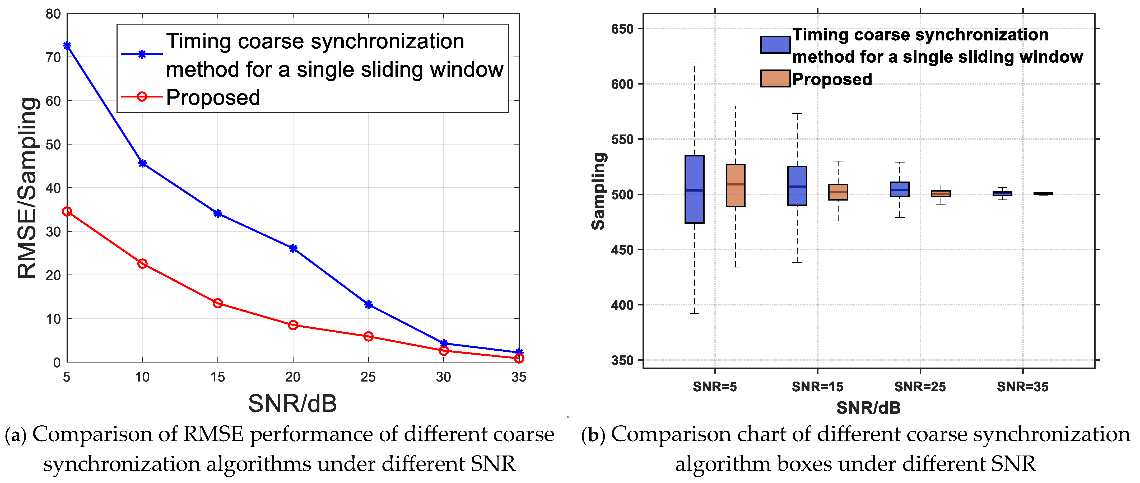
In simulation, RMSE is used to evaluate the performance of the algorithm, which is defined as:

$$RMSE=\sqrt{{\displaystyle \frac{{\sum }_{p=1}^P\mid {\widehat{\alpha }}_p-{\alpha }_{true}{\mid }^2}{P}}}$$

(67)

Among them, ${\alpha }_{true}$ represents the normalized true values of the CFO and STO, ${\widehat{\alpha }}_p$ represents the estimated value of the $p^{th}$ experiment, $P$ represents the number of independent Monte Carlo experiments, and the results are calculated using $P=500$.

As shown in the above Figure 6, the synchronization performance of the CP-based timing coarse synchronization detection method deteriorates with the decrease in signal-to-noise ratio, and the traditional single window timing detection method is more sensitive to changes in signal-to-noise ratio. In low signal-to-noise ratio environments, traditional methods not only have inaccurate coarse synchronization, but also have a large degree of estimation dispersion, making it difficult to obtain accurate and stable synchronization performance. This section adopts a multi-window joint estimation mechanism to accumulate group peaks, which not only improves synchronization accuracy, but also enhances the robustness of coarse synchronization, providing accurate and stable initial reference points for frequency offset estimation and fine timing synchronization, and improving time–frequency synchronization performance.

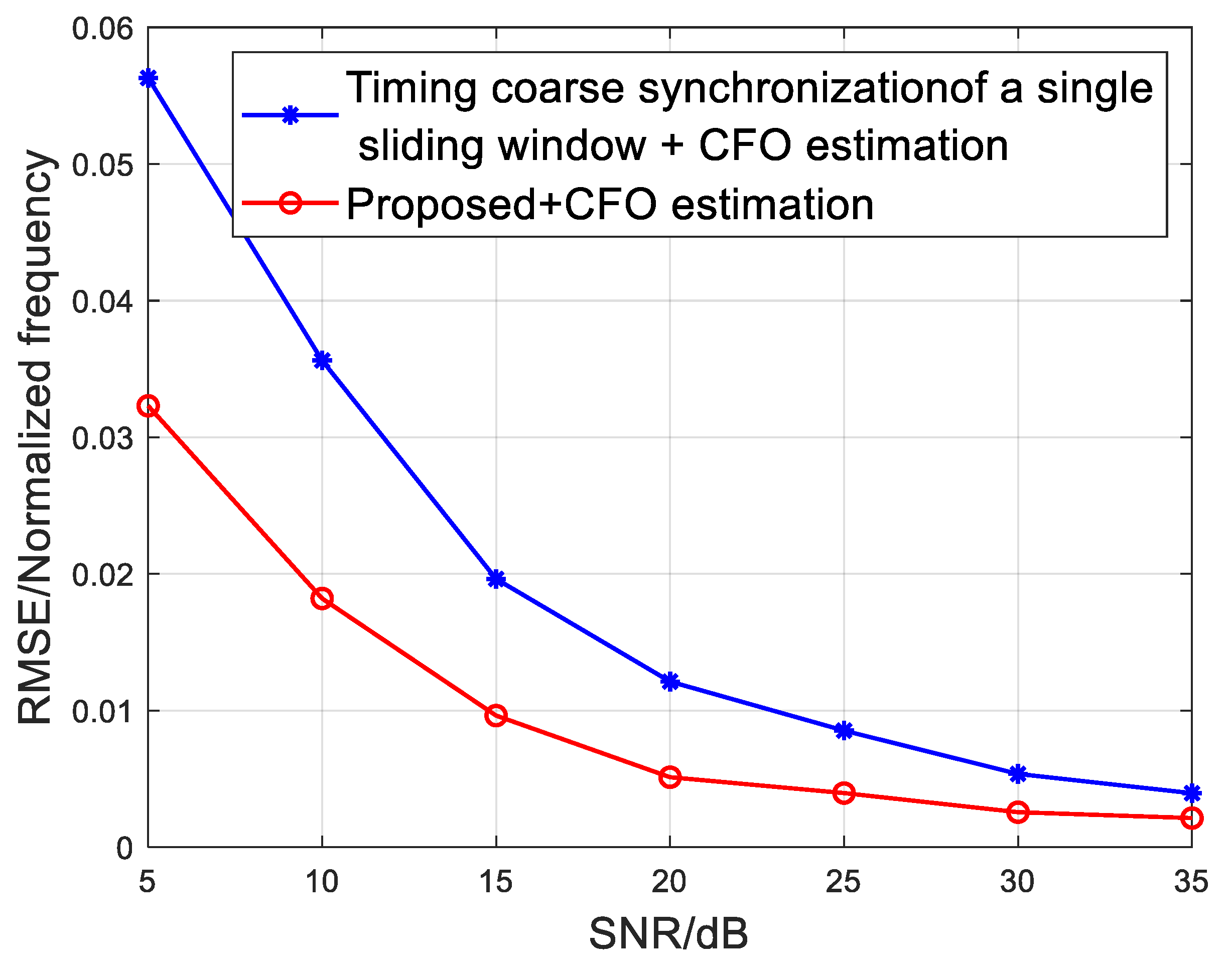
After performing coarse timing synchronization, it is necessary to estimate and compensate for the frequency offset. In the simulation, the normalized frequency offset is set to 0.25, and a CP-based method is used for frequency offset estimation. The SNR and RMSE of the normalized frequency offset are shown in the following Figure 7. The method proposed in this chapter has good timing coarse synchronization performance, which further affects frequency offset estimation and improves the accuracy of CFO estimation.

(2) Fine timing synchronization simulation and analysis

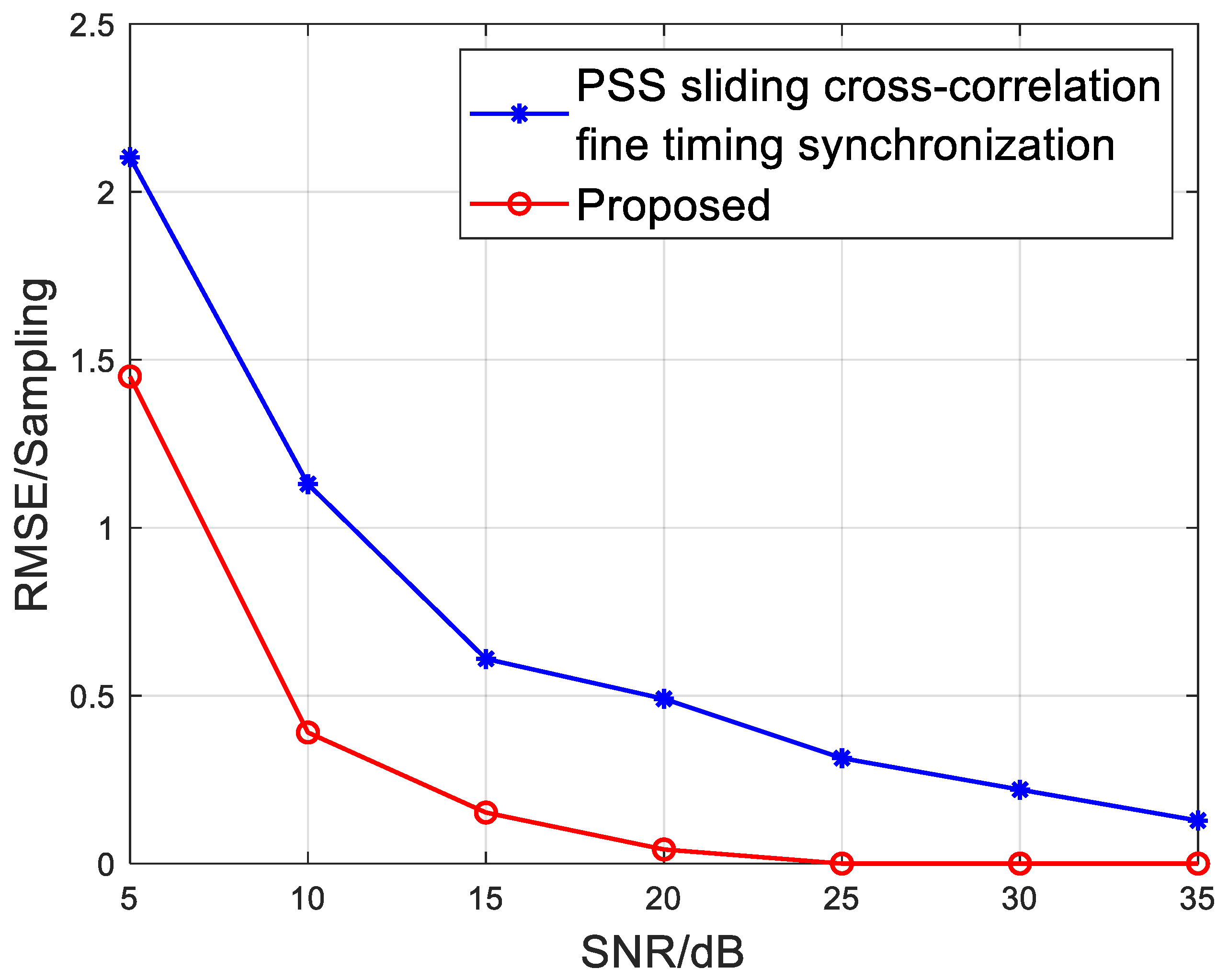
After estimating the CFO, the frequency is compensated to obtain corrected frequency information, and a fine timing synchronization method based on the PSS sliding cross-correlation is used. The CP-based timing synchronization method cannot achieve fine synchronization due to the short length and poor correlation of the CP sequence. Therefore, this section compares the PSS sliding cross-correlation synchronization method with the three-level time–frequency synchronization method based on group peak timing tracing proposed in this chapter, as shown in the following Figure 8. The PSS sliding cross-correlation synchronization method can achieve accurate synchronization accuracy, but due to its lack of frequency offset elimination, its timing synchronization accuracy is slightly lower than the algorithm proposed in this chapter. At high signal-to-noise ratios, the algorithm proposed in this chapter can synchronize to sampling accuracy. Even at low signal-to-noise ratios, the algorithm can achieve accurate synchronization accuracy and has precise and robust synchronization performance.

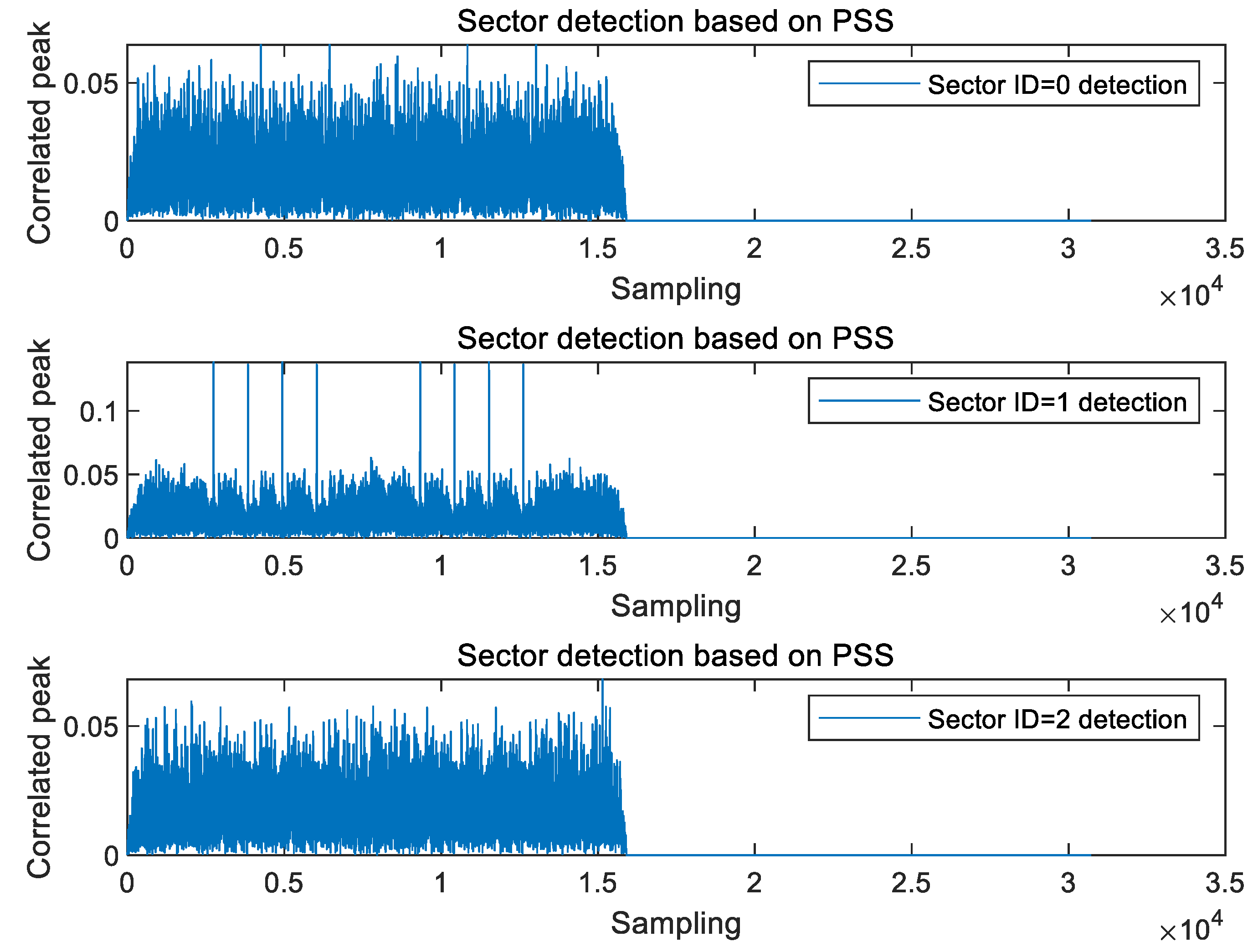
The PSS-based correlation operation can not only perform timing synchronization, but also search for sectors. The search results are shown in the following Figure 9. The Cell ID of this simulation is 16, corresponding to $N_{ID}^{\left(2\right)}=1$. When using this sequence for correlation operation, obvious peaks can be found.

5.2. Performance Verification of the Robust and Accurate Tracking Algorithm Based on the PRS

After synchronizing the PRS to chip accuracy, fine tracking is required to obtain ranging information with intra chip accuracy. This section verifies the tracking performance of the PRS through MATLAB 2023 environment simulation, and the resource allocation for 5G is shown in the following

Table 2. Parameter setting based on PRS ranging.

Parameter	Value	Parameter	Value
Carrier frequency	3.5 GHz	Fast fourier transform point number $N_{\mathrm{F}\mathrm{F}\mathrm{T}}$	4096
Subcarrier spacing	60 kHz	Number of resource blocks	272
PRS resource set period $T_{\mathrm{per}}^{\mathrm{PRS}}$	4	PRS resource repetition cycle $T_{\mathrm{rep}}^{\mathrm{PRS}}$	4
PRS symbol number $L_{\mathrm{PRS}}$	12	Cyclic prefix mode	normal
Comb count $K_{\mathrm{comb}}^{\mathrm{PRS}}$	2

:

To improve time-domain resolution, a larger subcarrier spacing and number of fast Fourier transform points are required. Therefore, the subcarrier spacing SCS is set to 60 kHz, and the number of fast Fourier transform points $N_{\mathrm{F}\mathrm{F}\mathrm{T}}$ is set to 4096. Currently, the length corresponding to each chip is ${\displaystyle \frac{c}{SCS\times N_{\mathrm{F}\mathrm{F}\mathrm{T}}}}={\displaystyle \frac{3\times {10}^8}{60\times {10}^3\times 4096}}\approx 1.22 \mathrm{m}$. To improve tracking performance, it is necessary to increase the number of symbols of the PRS in one time slot as much as possible. In this section, the maximum value is taken to make $L_{\mathrm{PRS}}=12$.

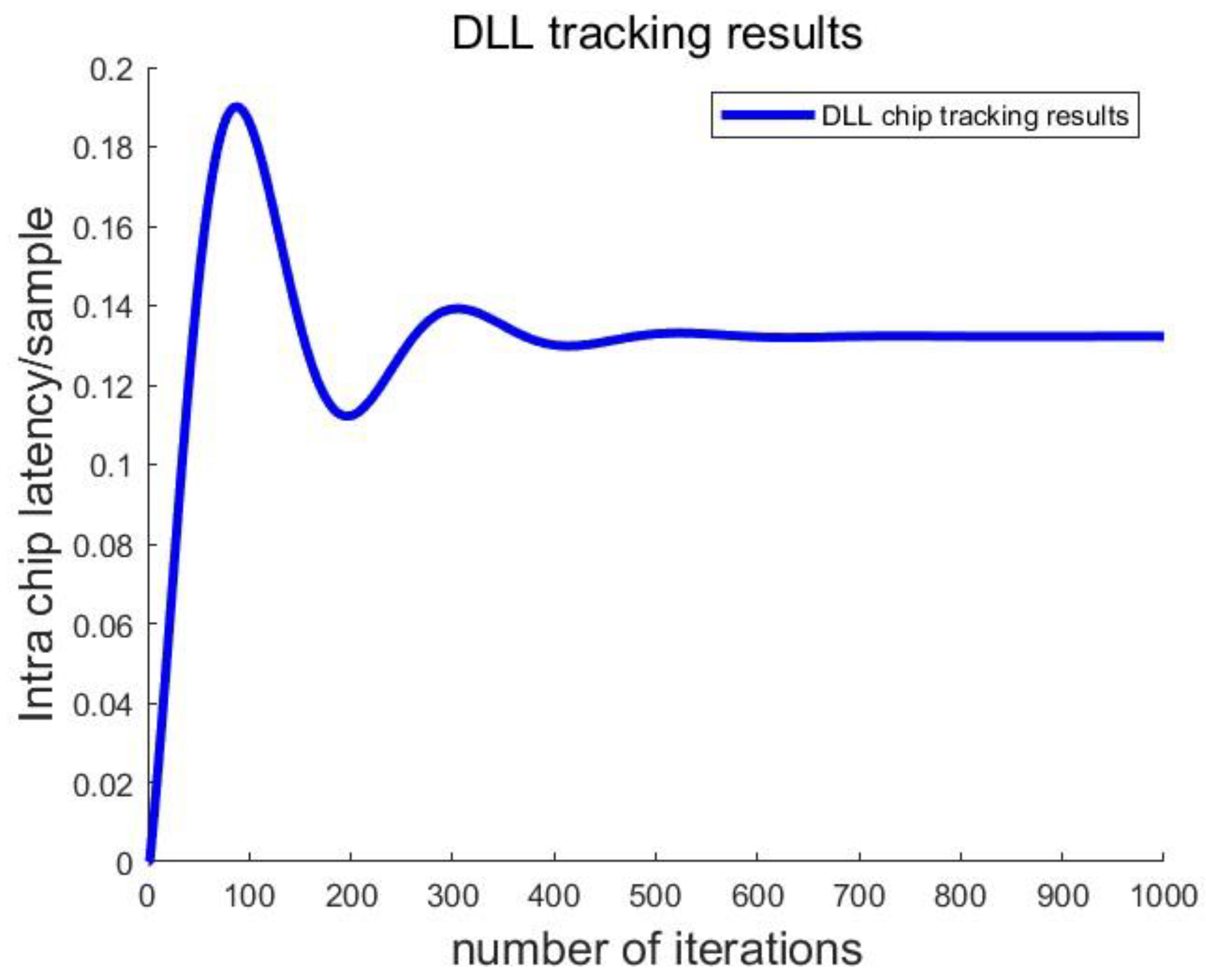
In the simulation process, assuming that the distance between the base station and the terminal is 27 m, with a length of approximately 22.12 chips, to verify the tracking performance of the tracking loop on the PRS, a time delay error of decimal times the sampling interval is added to the OFDM symbols that have not yet been sent by the base station, which can be expressed as:

$$X_{i,n}=X_{i,n}{e}^{-2\pi (n-1)\mathrm{F}\mathrm{r}\mathrm{a}/N_{\mathrm{F}\mathrm{F}\mathrm{T}}}$$

(68)

Among them, $Fra=0.1184$ represents the delay error of decimal times the sampling interval, and the tracking result is shown in the following Figure 10.

After a certain number of iterations, the loop can track up to 0.13 chips, and the ranging accuracy is better than 0.1 m.

5.3. Performance of the Fusion Localization Algorithm

The location coordinates of the base station are shown in the following

Table 3. Base station coordinate setting.

Parameter	Value	Parameter	Value
Base 1	[10 m, 10 m, 3 m]	Base 4	[10 m, 30 m, 3 m]
Base 2	[30 m, 10 m, 3 m]	Base 5	[30 m, 30 m, 3 m]
Base 3	[50 m, 10 m, 3 m]	Base 6	[50 m, 30 m, 3 m]

:

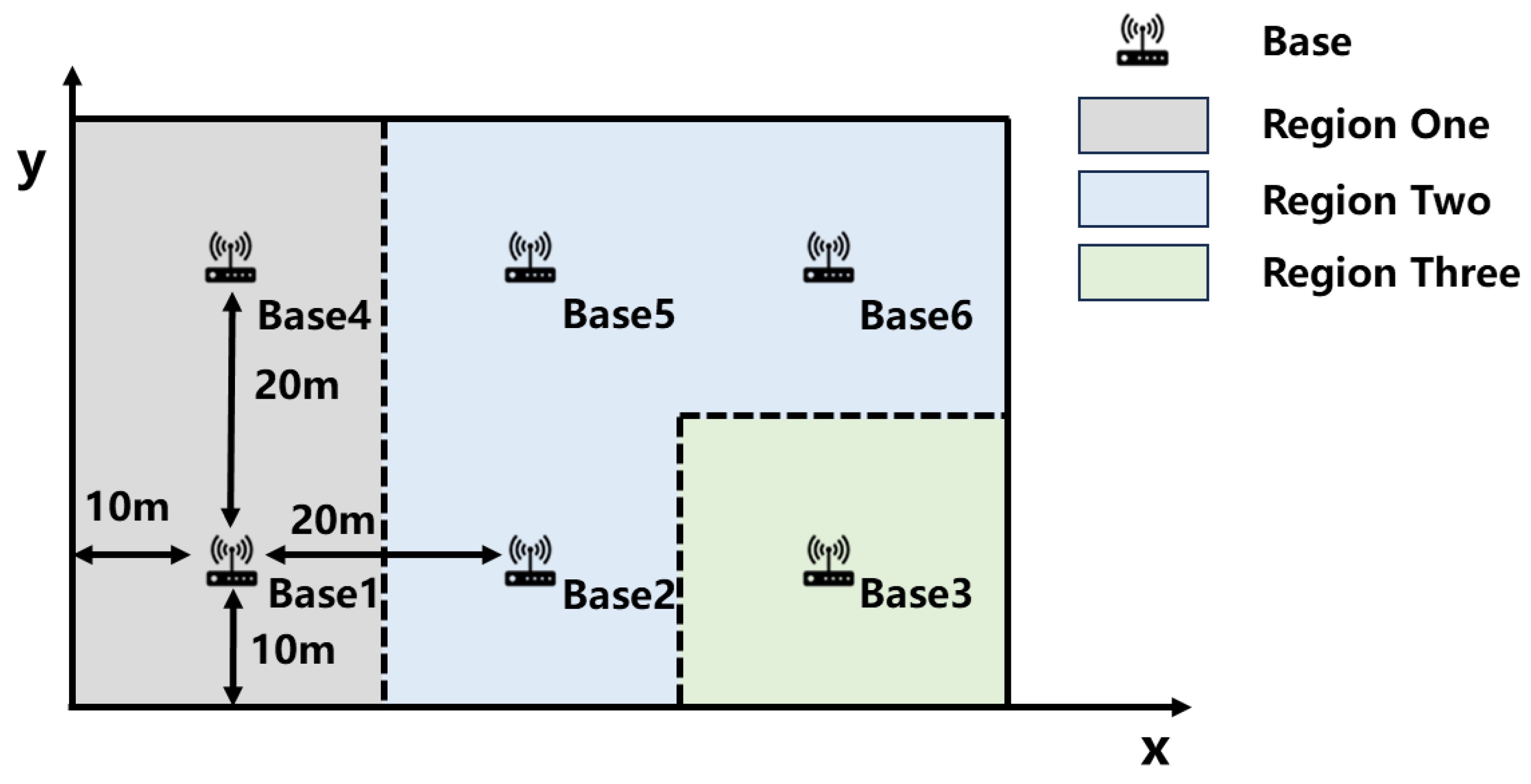
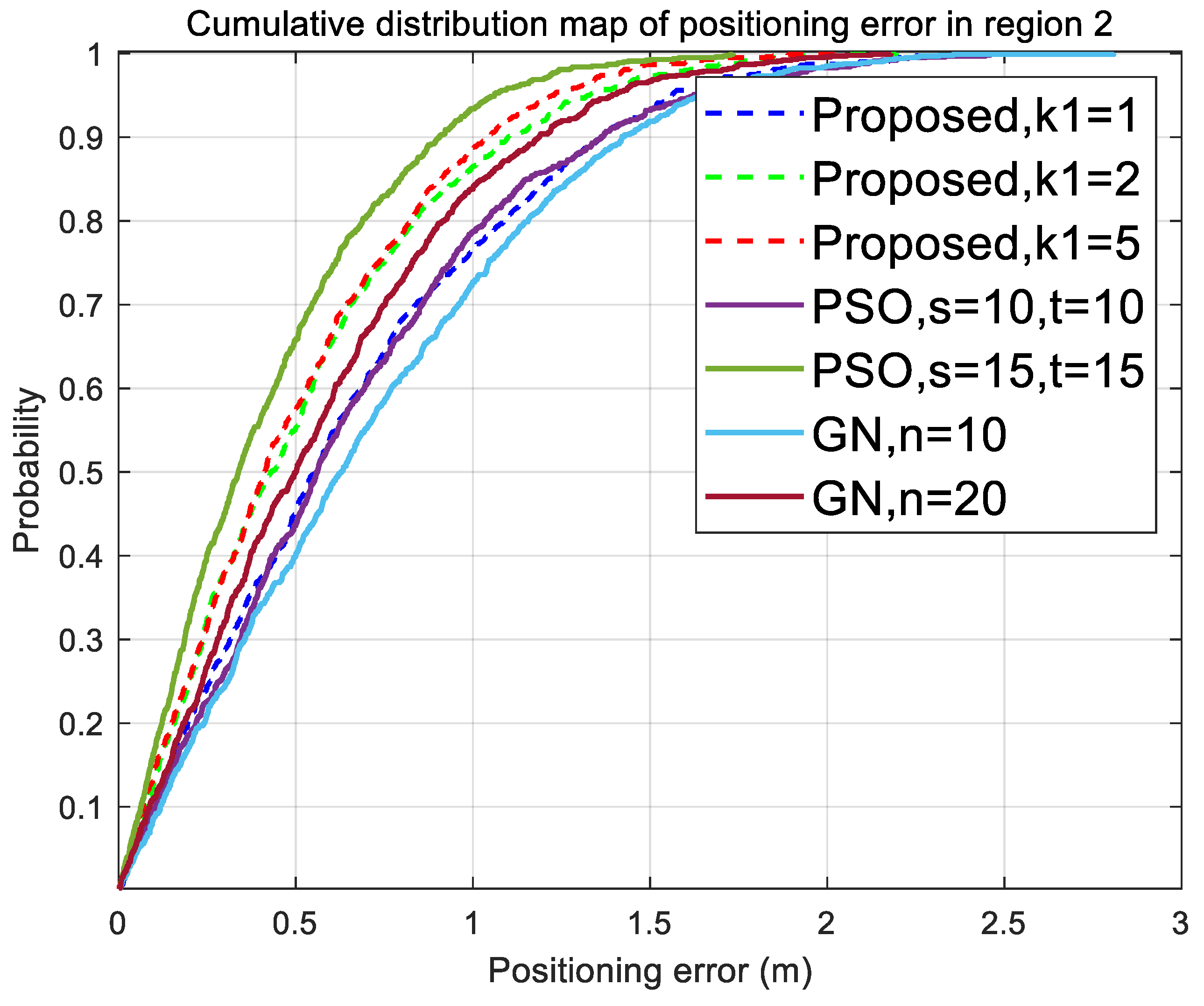
The layout of the base station is shown in the following Figure 11. The entire factory area is divided into three regions, each of which is affected differently by non-line of sight, resulting in different amounts of available positioning observation information received in different regions. The positioning performance of the three scenarios is compared and analyzed to verify the performance of the continuous positioning algorithm proposed in this chapter. Assuming that in region one, the propagation paths of base stations 1, 2, and 4 are direct paths, but due to hardware limitations, only the angle information of base station 1 can be measured. In Region 2, the propagation paths of base stations 2, 4, 5, and 6 are direct paths, and each direct path can obtain accurate angle information; In region three, only base station 3 has a direct path and can measure angle information. In the process of algorithm performance verification, the positions of positioning terminals are randomly generated in three different areas, and the measurement results are calculated using the algorithm in this chapter and the comparative algorithm. The positioning errors are then statistically analyzed.

To verify the progressiveness of the algorithm in this paper, the current mainstream Gauss–Newton (GN) algorithm and the Particle Swarm Optimization (PSO) algorithm are added as comparative experiments. In the positioning process, the NLOS recognition method based on comprehensive feature dynamic hierarchical optimization is first used to determine the non-line of sight path, and the LOS path is selected for high-precision measurement. The robust accurate tracking algorithm based on the PRS is used to obtain the downlink ranging information, and the efficient angle measurement algorithm based on fourth-order cumulants is used to obtain the uplink angle information. The angle and distance information are uploaded to the network side for positioning calculation. The initial position of the Gauss–Newton method is obtained through the ordinary least squares method, and the initial position of the particle swarm optimization algorithm is randomly generated and gradually iterated within the area where the positioning terminal is located. In the algorithm proposed in this article, the closed-form solution is first solved using the generalized least squares method. Since the covariance matrix of the error in the initial state is unknown, the identity matrix needs to be used as the initial weight matrix to obtain a more accurate closed-form solution through a few iterations, with the number of iterations represented by $k_1$. This experiment conducted 1000 Monte Carlo experiments, using the cumulative distribution function of positioning errors as the evaluation index for positioning performance.

Region 1 and Region 2 belong to areas with good wireless signal coverage performance, satisfying geometric observability and having many redundant observations. From the above Figure 12 and Figure 13, the closed-form solution obtained after a few iterations can have good localization performance, which is superior to the PSO algorithm and GN algorithm with few iterations. With the increase in iteration times, the localization performance of both the proposed algorithm and the comparative algorithm has been improved. As the number of particles increases, PSO has higher positioning accuracy in the case of more observation information (region two). However, in complex scenarios, not all regions have a lot of redundant observation information. In region one, there are fewer redundant observations, and the number of effective particles will accelerate decay. After resampling, the diversity of particles will decrease, and the ability to explore the state space will weaken, making it easy to fall into local optima and resulting in a decrease in localization performance. At this point, the algorithm proposed in this article fully explores the relationship between angle and distance, and has high positioning robustness. Even with less redundant observation information, it can provide high positioning accuracy.

6. Conclusions

This paper proposes a three-stage time–frequency synchronization method based on group peak time sequence tracking. In the first stage, coarse timing synchronization is achieved via group peak accumulation timing coarse synchronization algorithm for multi-window joint estimation. In the second stage, frequency offset estimation is performed using cyclic prefix correlation. Finally, fine timing synchronization at the chip level is realized through sliding cross-correlation with the primary synchronization signal.

Furthermore, a multimodal positioning algorithm is introduced for heterogeneous measurement fusion in 5G systems. By employing high-precision angle-of-arrival observations as intermediate variables, a linear observation model is constructed. Modeling and analysis are conducted for various multimodal scenarios, leading to a closed-form solution of the position information. This approach enables robust and high-precision positioning performance, even under dynamic conditions with varying types and quantities of observations.

Future work will focus on integrating 5G with inertial navigation systems to achieve continuous and robust positioning in complex environments.