A Study on Small-Scale Snake Image Classification Based on Improved SimCLR

Abstract

The exotic pet trade is a major driver of alien species invasions. Improper introductions or a lack of management can result in severe ecological consequences. Therefore, accurate identification of exotic pets is essential for the prevention and early warning of species invasions. This paper proposes a novel recognition method for fine-grained images of small-scale exotic pet snakes in complex backgrounds based on an improved SimCLR framework. A hierarchical window attention mechanism is introduced into the encoder network to enhance feature extraction. In the loss function, a supervised contrastive mechanism is introduced to exclude false negative samples using label information, which helps reduce representation noise and enhance training stability. The training strategy incorporates random erasing and random grayscale data augmentation techniques to improve performance further. The projection head is constructed using a two-layer multilayer perceptron (MLP), and the cosine annealing schedule combined with the AdamW optimizer is adopted for learning rate adjustment. Experimental results on a self-constructed dataset demonstrate that the proposed model achieves a recognition accuracy of 97.5%, outperforming existing baseline models. This study fills a gap in exotic pet snake classification and provides a practical tool for species invasion prevention and early detection.

1. Introduction

Alien invasive species can cause a range of serious problems, including species extinction, degradation of natural ecosystems, and agricultural losses [1,2]. According to the United Nations Global Assessment Report on Biodiversity and Ecosystem Services, the number of alien invasive species in each country has increased by 70% since 1970, making it one of the five major drivers that have significantly impacted global ecosystems over the past 50 years. Due to its vast territory and diverse ecosystems, biological invasions have long affected China. These invasions have caused substantial losses to the agricultural and forest production of the country, and the associated costs of eradication and control are also considerable [3,4]. Many alien species have been introduced into new environments through international or regional trade. Exotic pets, in particular, may escape, be abandoned, or be intentionally released into the wild. In the absence of natural predators and due to their strong adaptability, such species may become invasive and cause severe damage to local ecosystems. China has launched the “4E Action Plan” to address this issue, which aims to combat species invasions effectively. The plan includes early-stage prevention, warning, monitoring, and detection; mid-stage eradication and interception; and late-stage joint control and disaster mitigation. Among these, detection and monitoring play a crucial role and involve techniques such as molecular identification, image-based recognition and diagnosis, remote intelligent monitoring, and regional tracking. At this stage, accurate species identification is essential. Introducing a classification model for exotic pet snakes can significantly improve operational efficiency at customs checkpoints. Real-time image-based analysis can help rapidly identify species and determine whether they are protected or prohibited from trade, thereby supporting efforts to combat illegal smuggling. Furthermore, such a classification model can help build a comprehensive species database, enabling customs to record information on each exotic pet that enters or leaves the country. This data-driven approach improves regulatory oversight and provides a scientific basis for developing more effective policies and preventive measures.

However, the current public datasets and image classification research of snakes, as well as the classification research mainly on venomous snake species, are used to assist in the diagnosis and treatment of snake bites [5,6]. In the past, fine-grained classification of snake images relied on expert classification and manual feature extraction on the dataset and did not develop [7]. With the continuous advancement of deep learning technology, the research on snake image classification has gradually increased in recent years. The current classification methods are divided into data enhancement, transfer learning [8,9], and multimodal data fusion, including the combination of snake bite images and geographic information [10,11,12,13,14].

Since 2019, there has been a growing focus on developing deep learning algorithms designed explicitly for snake image detection, which has been driven by continuous advancements in deep learning technology [15]. Convolutional Neural Network (CNN) models have been widely applied in snake image classification, significantly contributing to progress in this field. In 2019, classical CNN architectures such as ResNet and VGG were used in the study by Fu et al. [16], demonstrating a strong ability to extract deep image features and substantially improve classification performance. Fu and colleagues further enhanced the ResNet model by introducing the BRC module, achieving an accuracy of 89.1% on a self-constructed dataset with 10,336 images across 10 snake categories. Durso et al. observed that the EfficientNet model also performs well in snake image classification tasks, owing to its efficient use of parameters [17]. In a more recent study in 2024, Naz et al. collected 400 images of four venomous snake species and several non-venomous species from the Indian region. They achieved an accuracy of 86% using the DenseNet121 model [5].

In 2020, Alexey Dosovitskiy et al. introduced the Transformer architecture to the field of computer vision. The Vision Transformer (ViT) demonstrated remarkable performance in image classification tasks and was subsequently adapted for snake image classification [18]. In 2021, He Can et al. proposed a twin network approach using a Swin Transformer as the backbone. They optimized feature extraction through contrastive learning, focusing on key visual features of snakes, such as scale texture and colour patterns. The backbone network was pre-trained through transfer learning on a fine-grained snake dataset and then used within the twin network framework. The two sets of feature vectors extracted by the twin network were compared and classified utilizing a metalearner, achieving 99.1% accuracy on a five-class dataset of 17,389 images [19]. In recent years, the SnakeCLEF competition has become a prominent benchmark for fine-grained snake species identification, typically under real-world, geographically diverse conditions. The 2022 winning solution proposed a powerful multimodal framework combining image and geolocation metadata with customized loss functions and ensemble techniques to address data imbalance and long-tail distribution [20]. In 2023, the top-ranked approach further integrated visual features with metadata priors using CLIP embeddings and employed seesaw loss and venom-focused post-processing to enhance safety-oriented classification [21]. More recently, the 2024 solution explored the potential of self-supervised visual Transformers for feature extraction under limited supervision, showing promising results in embedding-based classification [22].

Despite recent progress in snake image classification, several challenges remain unresolved in the specific context of exotic pet snake identification. First, publicly available datasets focused on exotic pet species are lacking. The limited number of images and high visual similarity among species make it difficult for models to learn discriminative features. Second, many images are captured in complex environments with significant background interference, significantly affecting recognition accuracy. The current snake classification methods heavily rely on multimodal data and large-scale training, which may not be feasible for small sample scenarios. Our work focuses on this under-explored environment, aiming to improve snake recognition performance and achieve fine-grained classification of exotic snakes using only image data optimized for small datasets and contrastive learning frameworks.

Specifically, the contributions of this paper are as follows:

1. We propose a novel method for small-scale image classification in complex scenes based on supervised contrastive learning. This approach offers an efficient technical solution for rapid unpacking inspection in environments such as customs and security screening. It improved classification accuracy by 6.63% compared to traditional deep learning models.

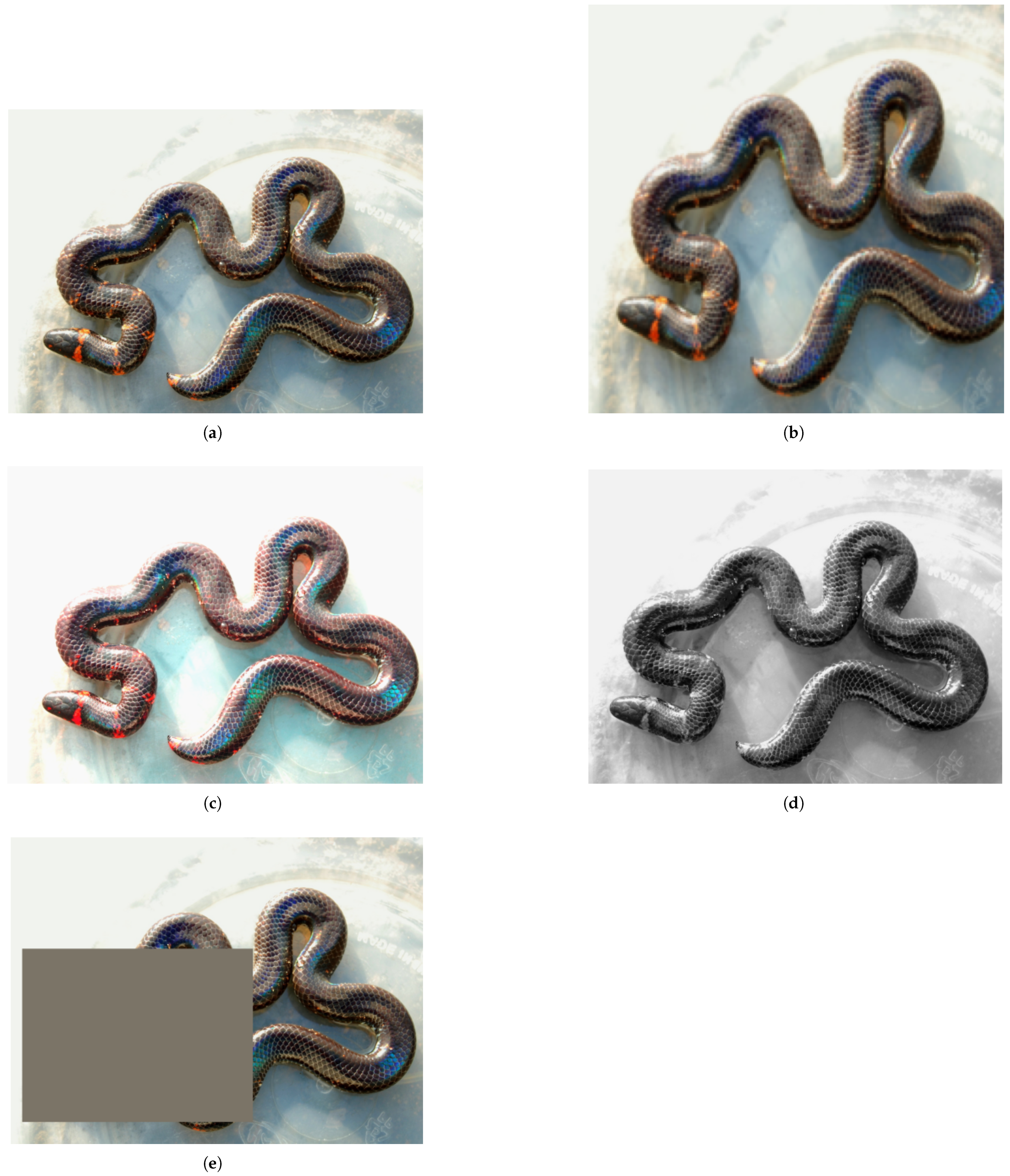
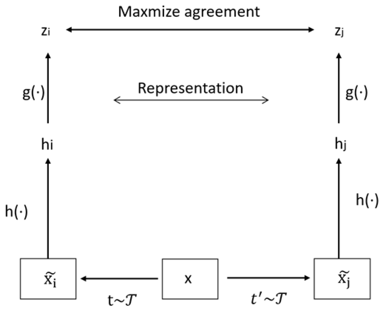
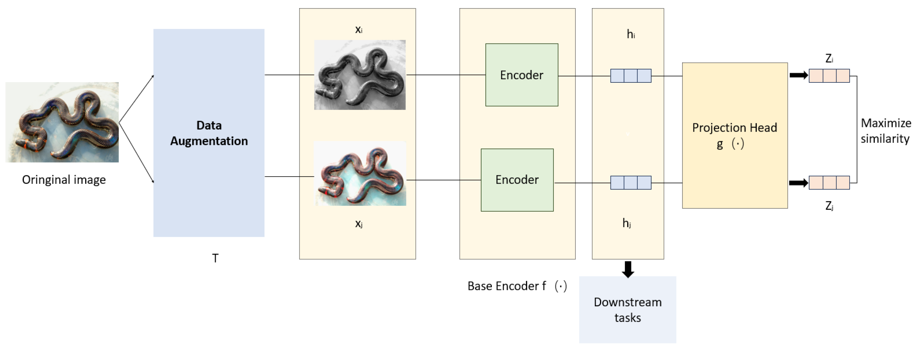
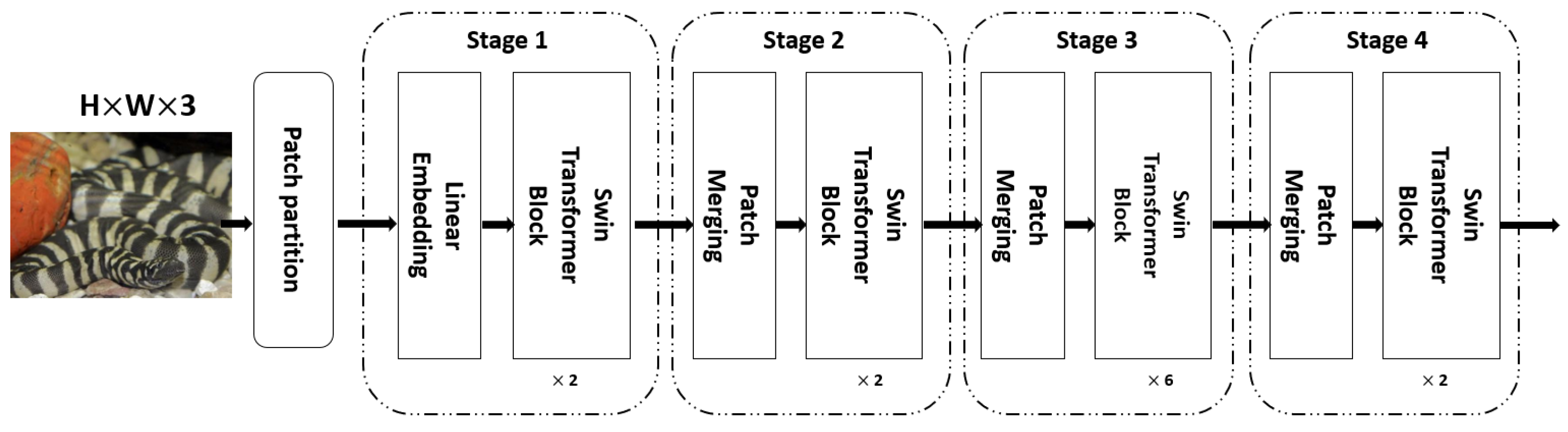
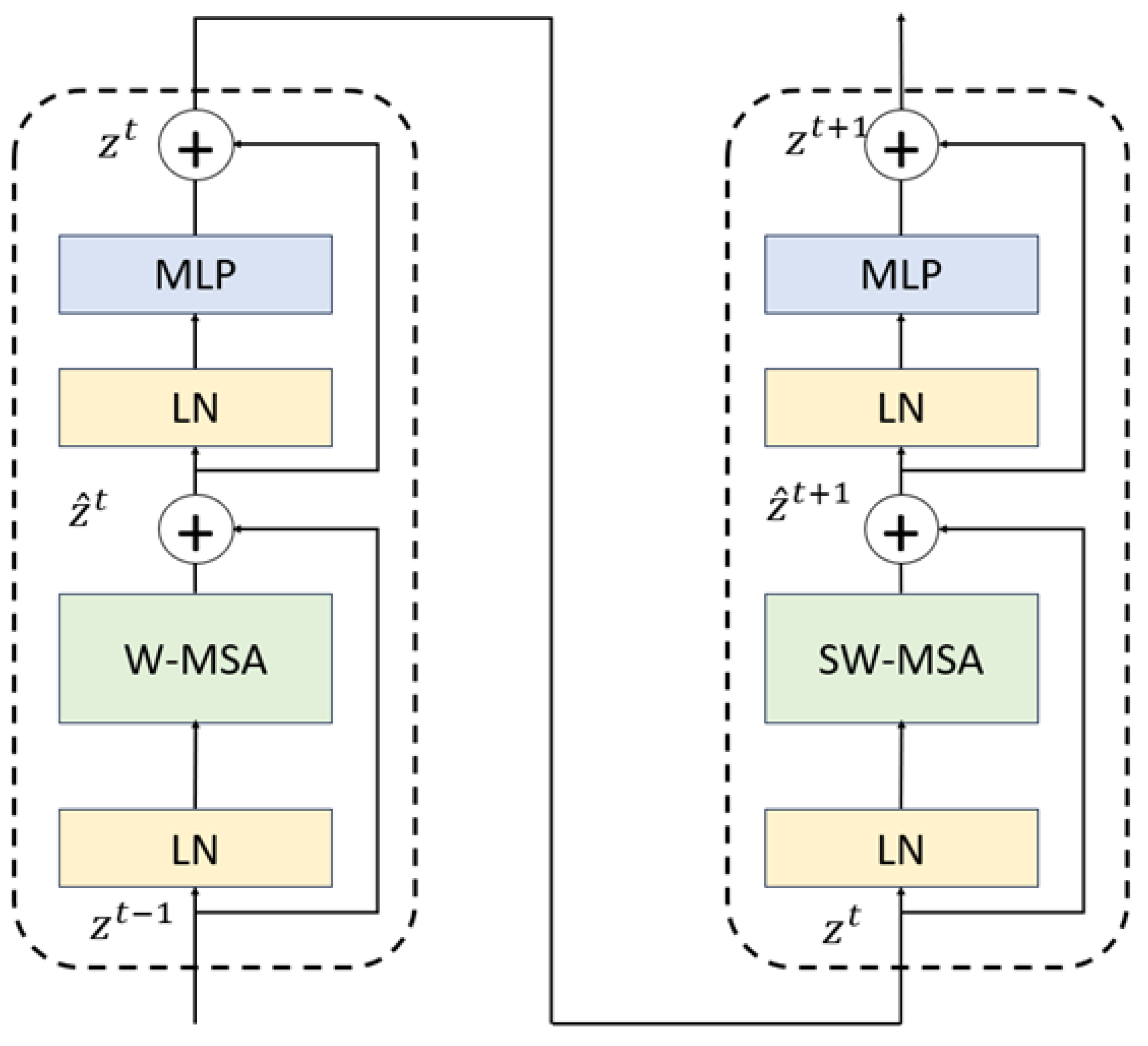
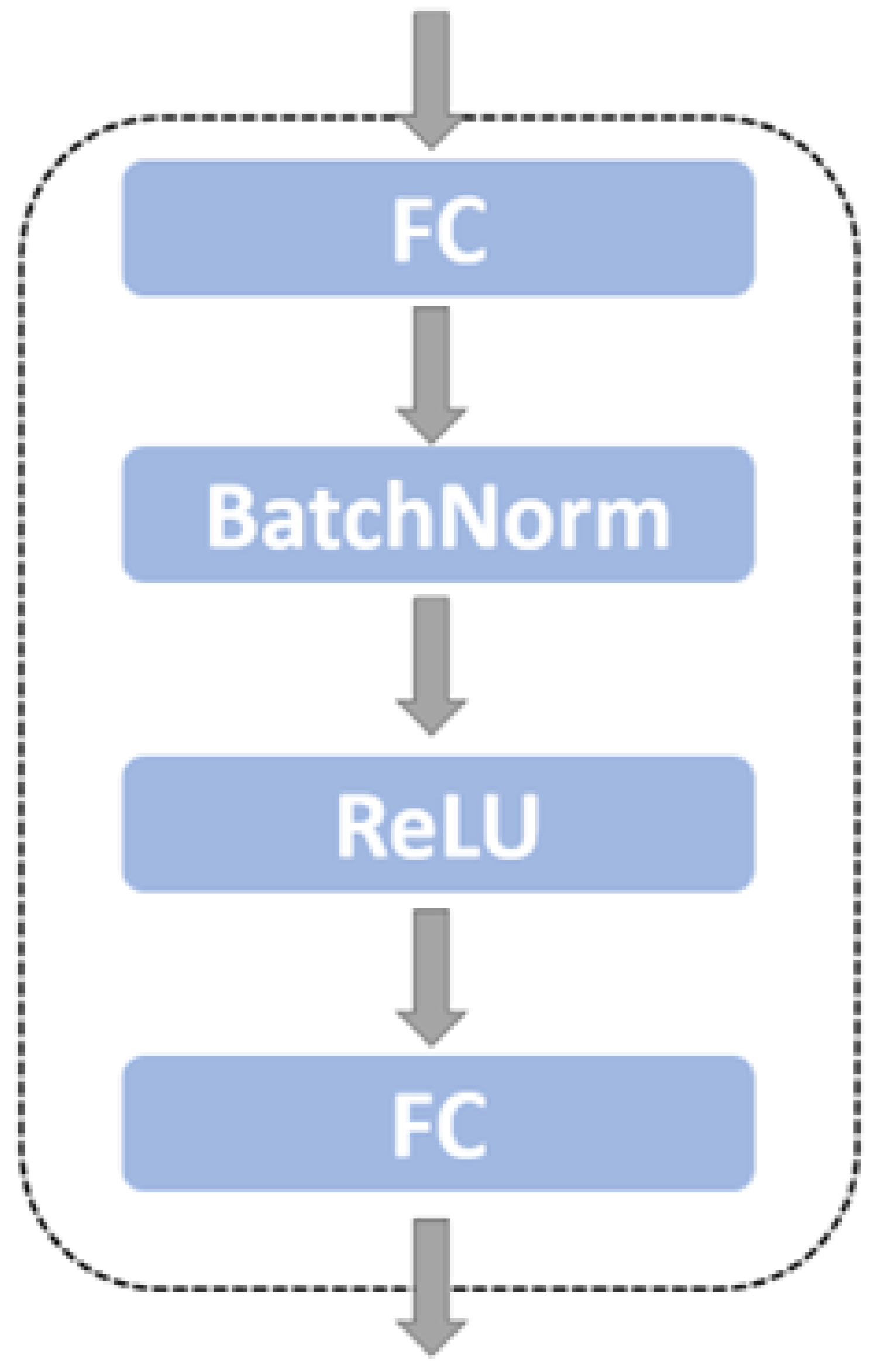
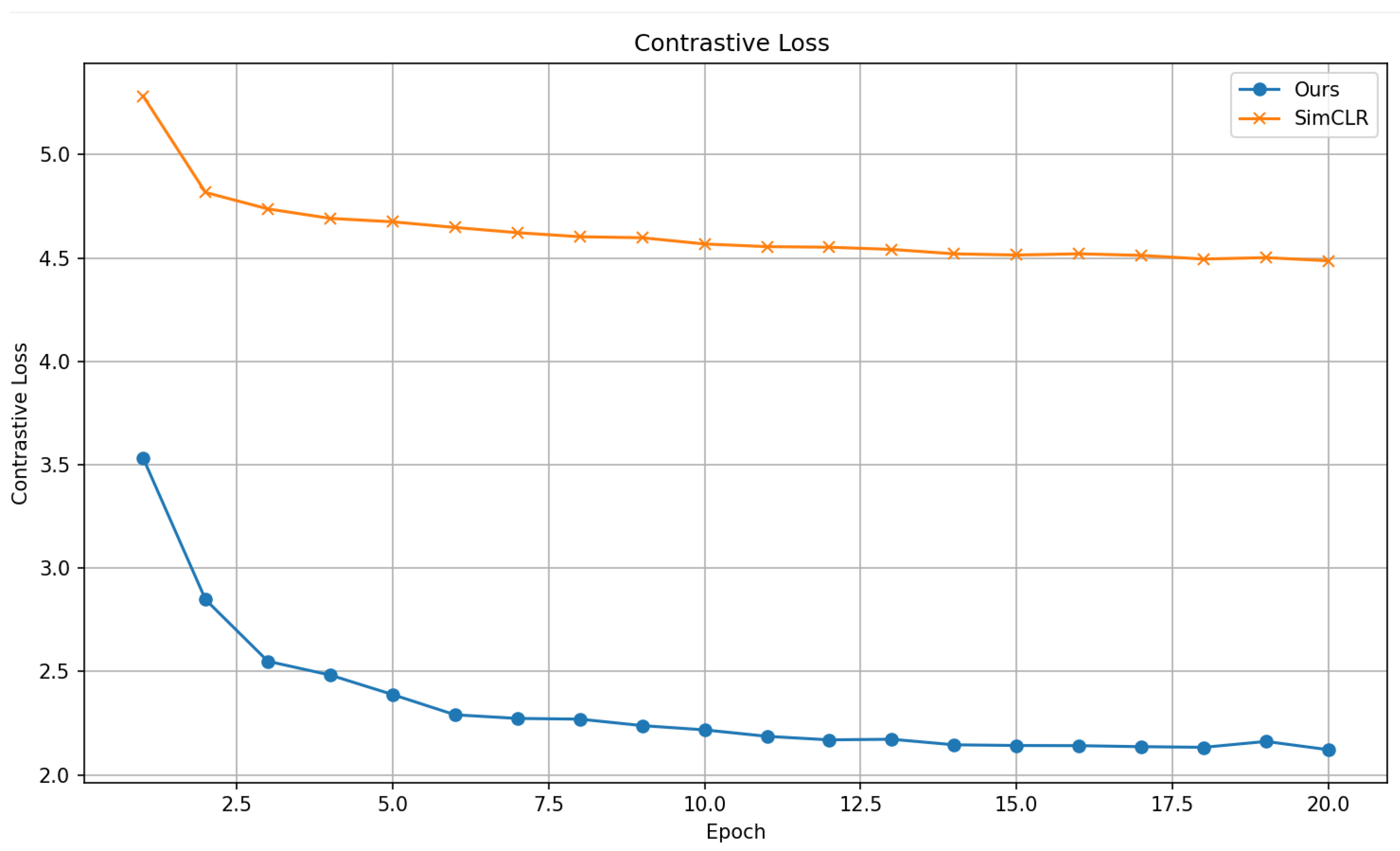
2. We improve the traditional SimCLR framework to better suit small-scale datasets with complex backgrounds. In the data augmentation module, in addition to basic image transformation strategies, we introduce grayscale enhancement and random erasure techniques. These strategies simulate complex background interference and significantly improve the model’s robustness to background noise. In the feature encoding module, we replace the traditional convolutional neural network with a Swin Transformer based on a shifted window multihead self-attention mechanism. This enables the model to leverage the advantages of global attention fully. The projection head is redesigned as a two-layer multilayer perceptron (MLP). For the loss function, a supervised contrastive mechanism is adopted. We employ the cosine annealing learning rate schedule and the AdamW optimizer regarding training strategy. This method achieved an accuracy of 97.48%, demonstrating superior performance in accuracy and relevance compared to other approaches in small-scale snake image classification.

3. We constructed a novel exotic pet snake image dataset comprising 17 species. Low-quality images are removed to ensure data clarity. This dataset can serve as a valuable reference for future research on exotic pet snakes or other tasks involving small-sample images with complex backgrounds.

2. Materials and Methods

2.1. Snake Image Classification

This dataset originates from the iNaturalist website. We independently collected image data for 17 snake species. The images were acquired under natural conditions and exhibit characteristics of field collection, such as complex backgrounds and varying lighting conditions, resulting in a certain degree of noise and distribution that reflects real-world scenarios. During the data collection process, we manually filtered the images to remove those that were blurry or heavily occluded, ensuring clarity and completeness to enhance overall image quality.

Despite these efforts, the dataset presents challenges, notably background interference, limited sample size, and subtle interspecies differences. First, background interference is a significant issue. Snake images are typically taken in natural environments with diverse and complex backgrounds, such as grass, rocks, soil, and other terrain, which often share similar colors and textures with the snake’s body. This resemblance can blur the distinction between the foreground and background, complicating visual recognition and making conventional CNN models more susceptible to background noise, thereby reducing classification performance. Second, the limited dataset size constitutes a significant constraint. Although the number of images per species ranges from 30 to 120, this quantity is generally insufficient for training deep learning models, particularly convolutional neural networks, and may easily lead to overfitting. The scarcity of training data makes it difficult for models to learn representative and robust features, negatively affecting classification accuracy. This issue becomes even more pronounced when dealing with many visually similar species, as the limited data exacerbate the complexity of the task. Finally, the presence of minor interspecies variations poses a critical challenge. Many snake species exhibit only subtle differences in appearance, and distinguishing features such as color and texture are often not distinguishable, especially among species belonging to the same genus or family. This high degree of visual similarity increases the difficulty of classification. Traditional deep learning methods may struggle to capture these nuanced differences effectively, thereby hindering improvements in classification accuracy.

The composition of the snake image dataset used in this study is summarized in

Table 1. Snake database.

Serial Number	Species Name	Number of Pictures
1	Cylindrophis ruffus	63
2	Ahaetulla prasina	120
3	Euprepiophis conspicillata	47
4	Acrochordus granulatus	67
5	Ramphotyphlops braminus	109
6	Xenopeltis unicolor	110
7	Candoia aspera	30
8	Corallus hortulanus	100
9	Corallus caninus	43
10	Epicrates cenchria	93
11	Epicrates angulifer	44
12	Boa constrictor	100
13	Gongylophis conicus	120
14	Eryx johnii	80
15	Eryx jayakari	64
16	Charina bottae	100
17	Lichanura trivirgata	100

Image source: iNaturalist website.

. The dataset was divided into training and testing sets in a 4:1 ratio, and hierarchical partitioning was used to maintain consistency in the distribution of each category in different subsets. This experiment applied multiple strategies to alleviate the problem of overfitting under small-sample conditions. During the model training phase, a pre-trained Swin Transformer model was employed as the encoder network, with its parameters kept trainable to extract discriminative features suited to snake images through contrastive learning. At this stage, extensive data augmentation was applied, combined with the AdamW optimizer, weight decay, and gradient clipping, enhancing the model’s robustness and helping prevent overfitting. In the linear evaluation phase, to mitigate overfitting on limited data, the parameters of the Swin Transformer were frozen, and only a linear classification head was trained, thereby improving the model’s generalization ability.

2.2. Data Augmentation Strategy Optimization

In deep learning, data enhancement has emerged as a prevalent approach to enhance model generalization, particularly in scenarios involving limited datasets [23]. In addition to the commonly used data augmentation methods, including random shearing, random rotation, and color jitter, this paper added the enhancement methods of RandomGrayscale and Cutout to improve the feature decoupling ability of the model through the two dimensions of color space deconstruction and spatial feature perturbation. In the color feature dimension, RandomGrayscale achieves effective decoupling of color channels through random grayscale operations, and its mathematical essence lies in converting the RGB three-channel image into a single-channel grayscale image:

$$I_{gary}=0.299R+0.587G+0.114B$$

(1)

The linear transformation is based on human visual perception weights and weakens color-dominated features while preserving key texture information. This operation forces the convolutional network to shift from color-dominated shallow features to deeper features such as edges and shapes, which can effectively alleviate the performance degradation phenomenon caused by the offset of color distribution [24].

In the spatial feature dimension, the random erasing algorithm constructs a dynamic occlusion simulation model by performing random rectangle-based erasure to enhance the model’s robustness against localized distortions [25].

Given an original image I, a random rectangular region ${\Omega }_2\subset I$ is selected, with its area ratio uniformly sampled in a pre-defined range (typically 2–33% of the image area). A binary mask $M_{ij}$ is defined as

$$M_{ij}=\left\{\begin{array}{cc}0,\hfill & \mathrm{if}(i,j)\in {\Omega }_2\hfill \\ 1,\hfill & \mathrm{otherwise}\hfill \end{array}\right.$$

(2)

The masked region is filled with a random matrix R, where each pixel is independently sampled from a uniform distribution $R_{ij}\sim \mathcal{U}(0,1)$ or set to a constant value. The enhanced image $I_{\mathrm{erase}}$ is then computed as

$$I_{\mathrm{erase}}=I\odot M+R\odot (1-M)$$

(3)

where ⊙ denotes element-by-element multiplication, and R is broadcasted to match the shape of I. These image processing techniques are shown in Figure 1.

2.3. Related Network

2.3.1. SimCLR

Contrastive learning is a representation learning method widely adopted in deep learning in recent years [26]. This method focuses on learning. Contrastive learning is a representation learning method commonly adopted in deep learning in recent years [26]. This method focuses on learning standard features and distinguishing differences between non-similar instances. The fundamental premise is to map similar instances closer in the learning embedding space while mapping dissimilar instances farther away. This supports migration learning, which applies to small sample data. The process of contrast learning is shown in Figure 2, which deomstrates features between similar instances and distinguishing differences between non-similar instances. The fundamental premise is to map similar instances closer in the learning embedding space while mapping dissimilar instances farther away. This supports migration learning, which applies to small sample data.

SimCLR (Simulation of Contrast-Based Learning) is an unsupervised contrast learning framework proposed by Google [27]. It achieves efficient feature learning through data augmentation, projection headers, and contrast loss. Its core goal is to optimize the representation of images in feature space through contrast learning so that similar samples are closer together and different samples are more distinguishable from each other. As illustrated in the accompanying Figure 3, the contrast learning algorithm under the SimCLR framework comprises four primary components: an image enhancement module, an encoder network, a projection network, and a contrast loss function.

Contrastive learning is typically initiated with data augmentation, the objective of which is to enhance the variability of the data. Data augmentation techniques include cropping, flipping, rotating, random cropping, and color transformations. Subsequently, an encoder network is trained, into which the enhanced data are fed, with the encoder network mapping them to a latent representation space in which meaningful features and similarities are captured. The encoder network is typically a deep neural network architecture, such as a CNN for image data or a recurrent neural network (RNN) for sequential data. The network learns to extract and encode high-level representations from the augmented instances, which helps to distinguish between similar and dissimilar instances in subsequent steps. The projection network is then employed to refine the learned representation. It takes the output of the encoder network and projects it into a lower-dimensional space. This process reduces the complexity of the data and facilitates better separation of similar and dissimilar instances. The contrast learning objective is applied once the augmented instances have been encoded and projected into the embedding space. Contrast learning aims to maximize the agreement between positive samples and minimize the agreement between negative samples. The similarity between instances is typically measured using a distance metric, such as the Euclidean distance or the cosine similarity. Models are trained to minimize the distance between positive pairs and maximize the distance between antagonistic pairs in the embedding space. Contrastive learning employs a range of loss functions to define the objective of the learning process, with the loss function playing a pivotal role in guiding the model to capture significant representations and differentiate between similar and dissimilar instances. The specific process is shown in Algorithm 1 below.

Algorithm 1 SimCLR’s main learning algorithm

Require: Batch size N, temperature $\tau$, encoder f, projection head g, augmentation set $\mathcal{T}$

1: for each minibatch ${\left\{x_k\right\}}_{k=1}^N$ do   2:     for each $k\in \{1,\dots ,N\}$ do   3:         Sample augmentations $t\sim \mathcal{T}$, $t^{\prime }\sim \mathcal{T}$   4:         ${\tilde{x}}_{2k-1}=t\left(x_k\right)$, ${\tilde{x}}_{2k}=t^{\prime }\left(x_k\right)$   5:         $h_{2k-1}=f\left({\tilde{x}}_{2k-1}\right)$, $z_{2k-1}=g\left(h_{2k-1}\right)$   6:         $h_{2k}=f\left({\tilde{x}}_{2k}\right)$, $z_{2k}=g\left(h_{2k}\right)$   7:     end for   8:     for each $i,j\in \{1,\dots ,2N\}$ do   9:         $s_{i,j}={\displaystyle \frac{z_i^{\top }{z}_j}{\parallel z_i\parallel \parallel z_j\parallel }}$ 10:     end for 11:     Define loss: $\ell (i,j)=-log{\displaystyle \frac{exp(s_{i,j}/\tau )}{{\sum }_{k=1}^{2N}{\mathbb{1}}_{[k\ne i]}exp(s_{i,k}/\tau )}}$ 12:     Total loss: $\mathcal{L}={\displaystyle \frac{1}{2N}}{\sum }_{k=1}^N[\ell (2k-1,2k)+\ell (2k,2k-1)]$ 13:     Update f, g to minimize $\mathcal{L}$ 14: end for 15: return Encoder $f(·)$; discard $g(·)$

2.3.2. Improvements to the Feature Encoding Module

Transformer is a deep neural network with a self-attention mechanism proposed by the Google team [28], and it has a wide range of applications in Natural Language Processing (NLP). In 2020, Transformer was introduced into computer vision [18], and ViT demonstrated the image classification task. Swin Transformer is an improvement of the ViT series [29], which improves the problem of high computation and poor fine-grainedness of ViT networks. The model under discussion is a visual Transformer model based on a Window Self-Attention mechanism. The sliding window mechanism is adopted to capture both local and global features. This results in a low computational complexity and an improvement in the efficiency of feature extraction. In this study, we adopted the Swin Transformer as the feature extractor in the contrast learning framework to enhance the model’s capacity to characterize images of exotic snakes. The structure of Swin Transformer is illustrated in the Figure 4, which is divided into four phases. Initially, the Patch partition divides the image into equal-sized image blocks, and then the image is flattened in the channel direction. Linear Embedding embeds the image blocks and changes them linearly, and then the deep features of the image are gradually extracted through several Block, Block, and Patch Merging operations [30].

We used Swin Transformer as the backbone network and removed the final classification layer to obtain a 1024-dimensional global feature vector. We then designed a projection head for mapping high-dimensional features onto a low-dimensional contrast space to optimize the contrast loss computation, which consists of a two-layer fully connected network.

1. Multiple self-attention mechanisms based on shift windows

The window-based multihead self-attention module (W-MSA) and the sliding window multihead self-attention module (SW-MSA) are the core parts of the Swin Transformer block. The specific structure is shown in the Figure 5:

Among them, ${\widehat{z}}^t$ and $z^t$ represent the output features of the (S) W-MSA module and the MLP module of the t-th block, respectively, where LN stands for layer norm layer, and MLP stands for multilayer perceptron. The LN module normalizes the input features, ensuring training stability and faster convergence.

The W-MSA module segments the input feature map into fixed-size, non-overlapping windows and applies self-attention independently within each window. This local attention design significantly reduces the computational complexity from quadratic to linear concerning image size while still allowing the model to capture rich local dependencies.

To compensate for the limited receptive field caused by the non-overlapping nature of W-MSA, the SW-MSA module introduces a window shift mechanism. Specifically, it shifts the window partitions by a fixed offset before applying attention. This causes each token to interact with new neighbors across window boundaries in alternating layers, enabling cross-window connections and allowing information to propagate beyond local regions.

Overall, the alternating use of W-MSA and SW-MSA modules allows Swin Transformer to model local and global relationships in visual data efficiently, balancing computational efficiency with representational power.

2. Projection head

Within the framework of contrastive learning, the projection head is pivotal in establishing a connection between the backbone network and the contrastive loss. This paper adopts a non-linear projection structure comprising two fully connected layers. This is shown in the Figure 6 below.

Firstly, the 1024-dimensional features extracted by the Swin Transformer backbone network are compressed to 512 dimensions through a linear transformation layer. This dimensionality reduction helps eliminate redundant information and improves computational efficiency.

Secondly, a Batch Normalization (BatchNorm) layer is applied to normalize the intermediate feature distribution, thereby accelerating convergence and alleviating internal covariate shifts. This operation also implicitly normalizes feature magnitude, making the contrastive loss more sensitive to angular similarity rather than feature scale [31].

The normalized features are then passed through a ReLU (Rectified Linear Unit) activation function, which introduces non-linearity and sparsity, helping enhance the discriminative power of the features by suppressing irrelevant information.

Finally, a second linear layer maps the features into a 128-dimensional contrastive embedding space, where similarity is measured via normalized cosine distances. No dropout is applied within the projection head to retain the full representation capacity during embedding learning.

2.3.3. Introduction of Supervised Loss Function

In SimCLR, the loss function is unsupervised and uses positive sample pairs generated based on data enhancement with unknown positive and negative sample labels. Positive sample pairs are generated through data enhancement, and feature representation is optimized with the help of the contrastive learning loss function. The formula is

$${\ell }_{i,j}=-log{\displaystyle \frac{exp\left(\frac{sim\left(z_i,z_j\right)}{\tau }\right)}{{\sum }_{k=1}^{2N}{1}_{\left[k\ne i\right]}exp\left(\frac{sim\left(z_i,z_j\right)}{\tau }\right)}}$$

(4)

However, for small-sample, high-similarity category tasks, reliance on unsupervised positive and negative sample partitioning may be inadequate due to the absence of intra-class features and an insufficient number of negative samples. The lack of explicit category information may result in samples of the same category being classified as negative. In contrast, the paucity of negative samples in a small dataset may compromise the efficacy of comparative learning.

In addressing these limitations, this paper proposes utilizing sample labeling information to ensure the aggregation of similar samples within the same category while promoting the separation of samples from different categories. This approach is formalized as a supervised loss function [32], the specific steps of which are outlined below:

1.

Feature normalization: The initial step involves the L2 normalization of the input feature vector to eliminate the effect of feature length. This ensures that the subsequent similarity calculation is contingent on the direction of the feature as opposed to the magnitude. Consequently, this process guarantees that the calculated similarity is consistent with the relative relationship between the samples:

$$features={\displaystyle \frac{features}{∥features∥}}$$

(5)

2.

Similarity calculation: The similarity matrix is then generated by calculating the cosine similarity between features:

$$similarit{y}_{matrix}=features\ast {features}^T$$

(6)

3.

Positive and Negative Sample Distinction: Within the framework of the loss function, labeling information is employed to explicitly differentiate between positive and negative sample pairs. Samples from the same category are designated positive sample pairs, whereas samples from different categories are classified as antagonistic sample pairs. A positive sample mask is constructed from the label information to ensure that the computation prioritizes the similarity between pairs of samples from the same category:

$$mask=labels={labels}^T$$

(7)

4.

Removal of the self-comparison effect: To avoid the effect of the similarity between the self-sample and itself in the calculation, we exclude the diagonal elements, i.e., the similarity between the sample and itself, by modifying the similarity matrix:

$$logits=similarit{y}_{matrix}-eye\left(n\right)\ast le12$$

(8)

5.

Loss function calculation: Finally, the contrast loss is optimized by calculating the ratio of the similarity of the positive sample pair to the similarity of all sample pairs. We use a temperature parameter to adjust the similarity scale and calculate the final loss through a logarithmic function and weighted average. The goal of this loss function is to minimize the similarity of sample pairs of the same category and maximize the similarity of sample pairs of different categories:

$$loss=-{\displaystyle \frac{1}{N}}\sum log\left({\displaystyle \frac{exp\left(logits\right)\ast mask}{ecp\left(logits\right)}}\right)$$

(9)

In actual model training, a fixed batch size of N = 64 was used, and each sample was generated into a positive view pair through two independent random enhancements. The same class samples within the batch were used as positive sample pairs using category labels. In contrast, samples of different categories in the batch were automatically treated as negative samples. The temperature hyperparameter was set to 0.07, referring to the default value in the SupCon Loss paper [32].

2.3.4. Optimization of the Training Strategy

The parameter update was performed using the AdamW optimizer, with the initial learning rate set to ${10}^{-4}$ and the weight decay coefficient set to ${10}^{-4}$. AdamW decouples the weight decay from the gradient update, effectively mitigating the risk of overfitting in the traditional Adam optimizer [33]. Concurrently, CosineAnnealing Learning Rate Scheduling is intended to facilitate the model’s escape from local optimal solutions and promote convergence to a more optimal generalization space [34].

These hyperparameters were selected based on prior empirical findings from the contrastive learning literature, such as SimCLR [27], which demonstrated that a learning rate of ${10}^{-4}$ and a temperature of 0.07 in the contrastive loss yield robust convergence across medium-scale datasets. The temperature parameter in the contrastive loss controls the concentration level of the similarity distribution, and 0.07 has been shown to provide a stable balance between gradient magnitude and optimization dynamics. A gradient clipping threshold of 1.0 was also applied to stabilize the training and further reduce overfitting risk under small-sample conditions.

1. Cosine annealing

The cosine annealing algorithm is an optimization strategy that dynamically adjusts the learning rate, and its core idea is to simulate the periodic decay process of the learning rate through the cosine function, given the initial learning rate ${\eta }_{max}$ and the cycle length $T_{max}$ at the t-th iteration is given by the learning rate formula:

$${\eta }_t={\eta }_{min}+{\displaystyle \frac{1}{2}}\left({\eta }_{max}-{\eta }_{min}\right)\left(1+cos\left({\displaystyle \frac{tmod{T}_{max}}{T_{max}}}\pi \right)\right)$$

(10)

where ${\eta }_{min}$ is the minimum learning rate, which decreases smoothly from ${\eta }_{max}$ to ${\eta }_{min}$ along the cosine curve in each cycle $T_{max}$, followed by an immediate restart to the initial value to start a new round of optimization. The periodic restart mechanism allows the optimization process to jump out of the current local minima and explore a more optimal convergence region, mitigating the risk of the gradient descent falling into a flat loss surface.

2. AdamW

The AdamW optimizer is an improved version of the Adam optimizer, which mainly addresses the misuse of weight decay in adaptive learning rate methods and is more suitable for Transformer architectures. In Adam, weight decay is implementationally equivalent to L2 regularization and is handled directly by merging the gradient update formulas:

$${\theta }_{t+1}={\theta }_t-\eta \ast {\displaystyle \frac{{\widehat{m}}_t}{\sqrt{{\widehat{\upsilon }}_t}+ϵ}}-\eta \ast \lambda {\theta }_t$$

(11)

where $\eta$ is the learning rate, and $\lambda$ is the weight decay coefficient. This coupling leads to weight decay being influenced by the adaptive learning rate, destroying its regularization nature.

AdamW explicitly separates weight decay from parameter updating, independent of the adaptive learning rate mechanism, as follows:

$${\theta }_{t+1}={\theta }_t-\eta \ast ({\displaystyle \frac{{\widehat{m}}_t}{\sqrt{{\widehat{\upsilon }}_t}+ϵ}}+\lambda {\theta }_t)$$

(12)

The weight decay term is no longer scaled by the adaptive learning rate and always acts on the parameters at a fixed scale. This is more in line with the original design intent of weight decay and improves the effectiveness of regularisation.

3. Results

3.1. Environment and Parameters

All experiments in this paper were conducted on Windows 11 (x64-based processor), the deep learning framework used was Python 3.12 and Torch 2.5.1, and the CPU was Intel(R) Core(TM) i7-14700H.

The detailed structure and parameters of the algorithm are shown in

Table 2. Architecture details of SwinContrastive and LinearProbe.

Module/Layer	Input → Output	Description	Activation/Regularization
SwinContrastive
Swin-Base Backbone	$3\times 224\times 224\to 1024$	Pre-trained Swin Transformer (ImageNet-1K), without frozen layers	LayerNorm, GELU (internal)
Linear	$1024\to 512$	First projection layer	None
BatchNorm1d	$512\to 512$	Normalize intermediate features	BatchNorm
ReLU	$512\to 512$	Activation function	ReLU
Linear	$512\to 128$	Final projection layer for contrastive head	None
Normalize (L2)	$128\to 128$	Normalize projection vector	${\ell }_2$ normalization
LinearProbe (Classifier)
Frozen Swin-Base Backbone	$3\times 224\times 224\to 1024$	Shared with contrastive model	Frozen
Linear	$1024\to 17$	Linear classifier head	None

and  

Table 3. Training hyperparameters used in contrastive and linear evaluation phases.

Phase	Hyperparameter	Value	Note
	Optimizer	AdamW	weight decay = $1\times {10}^{-4}$
	Learning Rate	$1\times {10}^{-4}$	constant base LR
Contrastive Pre-training	Scheduler	Cosine Annealing	$T_{max}=20$
	Epochs	20
	Batch Size	64
	Optimizer	AdamW	weight decay = $1\times {10}^{-4}$
	Learning Rate	0.01	higher LR for linear head
Linear Evaluation	Scheduler	None	fixed LR
	Epochs	15
	Batch Size	64

.

Furthermore, the model checkpoint corresponding to the highest validation accuracy was saved and used for final evaluation, effectively ensuring optimal model selection without manual intervention.

3.2. Evaluation Metrics

In this article, we used mainstream evaluation indicators such as accuracy, precision, recall, and F1-score to evaluate the effect of the model.

Accuracy is the most commonly used image classification performance indicator, representing the ratio of the number of samples correctly identified by the model to the total number of samples. The accuracy calculation formula is as follows:

$$Accuracy={\displaystyle \frac{TP+TN}{TP+FN+FP+TN}}$$

(13)

Precision reflects the ability to see how well the model distinguishes between positive samples and indicates the proportion of positive samples correctly identified by the model, as expressed by the following formula:

$$Precision={\displaystyle \frac{TP}{TP+FP}}$$

(14)

Recall represents the ratio of the number of samples correctly identified as positive by the model to the total number of positive samples, and the recall is calculated as follows:

$$Recall={\displaystyle \frac{TP}{TP+FN}}$$

(15)

F1 is the reconciled mean of precision and recall, an evaluation metric that combines precision and recall and is calculated using the following formula, where P is precision and R is recall:

$$F1={\displaystyle \frac{2PR}{P+R}}={\displaystyle \frac{2TP}{2TP+FP+FN}}$$

(16)

3.3. Experimental Results

3.3.1. The Impact of Data Augmentation Strategies

To investigate the effectiveness of different data augmentation strategies in contrastive pretraining, we conducted an ablation study, as shown in

Table 4. Impact of different data augumentation methods.

Data Augmentation Strategies	Accuracy	Training Loss
conventional augmentation methods	0.9676	2.1096
conventional augmentation methods + RandomGrayscale	0.9712	2.1207
conventional augmentation methods + RandomGrayscale + Random Erasing	0.9748	2.1211

. We started with conventional augmentation methods, including random resized crop, horizontal flip, color jitter, and Gaussian blur. This baseline set had already achieved a relatively high validation accuracy of 0.9676, indicating its ability to provide diverse and effective views for contrastive learning. Building upon this, we added the RandomGrayscale operation to simulate lighting and texture changes. This led to a modest but consistent improvement in accuracy to 0.9712, suggesting that the model benefited from learning invariant representations under grayscale transformations. Furthermore, we incorporated random erasing to simulate occlusion and background clutter. This yielded the highest accuracy of 0.9748, demonstrating that exposing the model to partially erased or corrupted views further enhances its ability to extract robust and generalizable features. Although training losses slightly increased across these configurations, this is expected due to the more challenging training samples and does not negatively impact downstream classification performance. These results highlight that progressively stronger data augmentation strategies, particularly those introducing appearance variation and local occlusion, are beneficial for learning discriminative representations in a contrastive learning framework.

3.3.2. Impact of Different Approaches

To evaluate the impact of different feature coding backbones on the contrastive learning framework, we compared three representative architectures—ResNet-50, ViT, and Swin Transformer—as summarized in

Table 5. Impact of different feature coding modules.

Feature Coding Module	Accuracy	Training Loss
ResNet50 (single split)	0.8705	2.1411
ViT (single split)	0.9532	0.2634
Swin Transformer (single split)	0.9748	2.1211
Swin Transformer (5-fold CV)	0.9811 ± 0.0015	–

.

The ResNet-50, a classical convolutional neural network, achieved a validation accuracy of 0.8705 with a relatively high training loss of 2.1411. While effective, it shows limitations in modeling long-range dependencies and complex structures, which may affect its capacity to learn discriminative representations in the contrastive setup. In contrast, the ViT architecture significantly outperformed ResNet-50 with an accuracy of 0.9532 and a notably lower training loss of 0.2634. This suggests that its global self-attention mechanism is better suited for capturing the holistic structure of snake images, even without convolutional priors. Further improvement was observed when using the Swin Transformer, which combines the advantages of both convolution and attention through a hierarchical window-based attention design. It achieved the highest accuracy of 0.9748, with a training loss of 2.1211. Despite the slightly higher loss than ViT, the Swin model demonstrates better generalization, likely due to its stronger inductive bias and better spatial locality modelling. In summary, Transformer-based feature encoders—particularly Swin Transformer—are more effective than conventional CNNs in contrastive learning for fine-grained snake species recognition, owing to their superior ability to capture global context and local structures.

To further evaluate the generalization of the Swin Transformer, we conducted a 5-fold cross-validation. As shown in Table 5, the model achieved an accuracy of 0.9811 ± 0.0015, surpassing the original single-split result of 0.9748, confirming the model’s robustness.

To further evaluate the classification performance of different backbone networks, we conducted a detailed per-class comparison using precision (P), recall (R), and F1-score metrics, as summarized in

Table 6. Performance comparison of ResNet50, ViT, and Swin Transformer.

Class	ResNet50			ViT			Swin-T			Support
	P	R	F1	P	R	F1	P	R	F1
1	1.00	0.87	0.93	0.79	1.00	0.88	1.00	1.00	1.00	15
9	0.82	1.00	0.90	1.00	0.93	0.96	1.00	0.93	0.96	14
10	0.81	1.00	0.90	1.00	1.00	1.00	1.00	1.00	1.00	13
11	0.70	0.54	0.61	0.91	0.77	0.83	1.00	0.85	0.92	13
12	0.95	0.90	0.92	1.00	1.00	1.00	1.00	1.00	1.00	20
13	0.83	1.00	0.91	1.00	1.00	1.00	0.95	0.95	0.95	20
14	0.77	0.67	0.71	0.85	0.73	0.79	1.00	0.87	0.93	15
15	1.00	0.75	0.86	1.00	1.00	1.00	0.94	1.00	0.97	16
16	0.73	0.95	0.83	0.80	1.00	0.89	0.91	1.00	0.95	20
17	0.89	0.94	0.91	1.00	1.00	1.00	1.00	1.00	1.00	17
2	0.94	1.00	0.97	1.00	1.00	1.00	0.94	1.00	0.97	17
3	0.92	0.75	0.83	0.91	0.62	0.74	1.00	1.00	1.00	16
4	0.94	1.00	0.97	1.00	1.00	1.00	1.00	1.00	1.00	16
5	1.00	0.72	0.84	1.00	0.94	0.97	1.00	0.94	0.97	18
6	0.67	0.86	0.75	0.95	0.95	0.95	0.95	1.00	0.98	21
7	1.00	0.60	0.75	0.82	0.90	0.86	0.91	1.00	0.95	10
8	0.94	0.88	0.91	0.89	0.94	0.91	1.00	1.00	1.00	17
Macro Avg	0.89	0.86	0.87	0.94	0.93	0.93	0.98	0.96	0.97	-
Weighted Avg	0.91	0.86	0.86	0.94	0.93	0.93	0.97	0.96	0.96

. The visual image is shown in Figure 7. The results demonstrate the superiority of Transformer-based models over the traditional convolutional backbone (ResNet50) in almost all categories.

1. Overall Trends:

The Swin Transformer achieved the highest macro and weighted averages of precision (0.98 and 0.97), recall (0.96 and 0.96), and F1-score (0.97 and 0.96), indicating robust performance and strong generalization across all classes. ViT followed closely with a macro F1-score of 0.93, significantly outperforming ResNet50, whose macro F1-score was only 0.87. ResNet50 showed inconsistent per-class performance, with some classes (e.g., Class 11, 7, and 6) exhibiting notably low recall and F1-scores, suggesting challenges in capturing subtle inter-class differences due to limited spatial context modelling.

2. Per-Class Observations:

Classes such as 10, 12, 13, and 17 were consistently classified with high precision and recall by all models, indicating that they are relatively easier to distinguish. For more challenging classes, such as Class 11 and Class 14, the Swin Transformer demonstrated remarkable robustness, achieving F1-scores of 0.92 and 0.93, respectively. In contrast, ResNet50 performed poorly (F1-scores of 0.61 and 0.71), likely due to its limited capacity to capture complex spatial patterns. ViT significantly improved over ResNet50 on difficult classes but occasionally suffered from reduced recall (e.g., Class 3 with R = 0.62), indicating some sensitivity to intra-class variance.

This comparative analysis confirms that Transformer-based feature extractors, especially Swin Transformer, are substantially more effective for fine-grained classification tasks like exotic snake species identification. Their ability to model global context and local details through attention mechanisms enables them to achieve higher precision, recall, and F1-scores across almost all classes. Swin Transformer achieved the best average metrics and exhibited the most stable and consistent performance across diverse classes.

In addition, this paper has also tried the traditional image classification methods, and the results are shown in

Table 7. Comparison with classical models.

Different Methods	Accuracy	Training Loss	Data Augmentation
ResNet34	0.8277	0.0012	10×
MoblieNetV3-L	0.8570	0.0059	10×
Efficientnetb04	0.9228	0.0043	10×
SimCLR	0.7662	4.3517	1×
Methodology of this paper (single split)	0.9748	2.1211	1×
Methodology of this paper (5-fold CV)	0.9811 ± 0.0015	–	1×

:

Compared to traditional CNN methods, the method proposed in this paper yielded significantly improved accuracy, which is 6.63% higher than the most effective netb04 network. The algorithm in this article does not require data expansion and uses fewer computational resources, making it more suitable for small datasets than traditional CNN networks. In addition, the method proposed in this article does not use multimodal data fusion and has lower requirements for the dataset. Compared to the unimproved SimCLR method, the accuracy has been significantly improved, and as can be seen from the loss curve in Figure 8, the supervised loss has improved convergence. In summary, compared to previous snake classification research methods, the improved supervised comparative learning method based on the SimCLR framework used in this paper has simpler requirements and more accurate classification results in the fine-grained classification of small-scale snakes.

4. Conclusions

This paper proposes an improved supervised contrastive learning model based on the SimCLR framework for fine-grained snake image classification under high-interference background conditions in a small-scale dataset. Our method introduces enhanced data augmentation strategies, including grayscale enhancement and random erasing, to simulate complex background interference and improve robustness. In the feature encoding module, we replace the traditional ResNet50 backbone with a Swin Transformer that leverages global self-attention for better spatial context modelling. Furthermore, a two-layer MLP projection head is designed to strengthen representation learning. The loss function adopts a supervised contrastive mechanism, and training uses cosine annealing scheduling with the AdamW optimizer.

Experimental results demonstrate that the proposed method achieved an accuracy of 97.48%, representing a significant improvement of 6.63% over traditional CNN models like EfficientNet-b4 while requiring fewer computational resources and no reliance on multimodal data or aggressive data augmentation. Additionally, we constructed a novel exotic pet snake image dataset of 17 species, providing a valuable benchmark for future research on small-sample, high-interference snake image classification.

Despite achieving good experimental results, we recognize that there are still directions for optimization in the current research. Firstly, due to the imbalance in the number of classes in the dataset, some classes contain as few as 30–40 images, which may limit the generalizability and robustness of the research results. Although data augmentation has somewhat alleviated this issue, more systematic class imbalance handling strategies can be explored in future work. Secondly, potential label errors in the dataset may affect the performance of supervised contrastive learning, and future research should consider incorporating anti-noise contrastive targets. Thirdly, although we assume this method may apply to other reptiles such as lizards and turtles, considering their similar data scarcity and complex image backgrounds, this hypothesis is still speculative and requires more experiments to verify.

In summary, our method offers an effective and efficient technical solution for fine-grained snake recognition in constrained and noisy environments, with potential applications in customs inspection, biosecurity, and exotic pet regulation. Future work will focus on expanding the dataset, improving robustness, and validating the method’s generalization to other species and domains.

References

1. Roy, H.E. IPBES Invasive Alien Species Assessment: Summary for Policymakers. Zenodo 2023. [Google Scholar] [CrossRef]
2. Du, Y.; Tu, W.; Yang, L.; Gu, D.; Guo, B.; Liu, X. Research Progress on the Impact of Invasive Alien Vertebrates on Biodiversity. Sci. China Life Sci. 2023, 53, 1035–1054. [Google Scholar]
3. Pang, J.; Liu, Y.; Chen, J. Current Status and Prevention System Construction of Invasive Alien Species: A Global Perspective and China’s Case. Chin. J. Agric. Resour. Reg. Plan. 2024, 45, 131–140. [Google Scholar]
4. Wang, S.; Li, Z.; Wang, Z.; Zhang, M.; Xu, J.; Liu, R. Distribution Pattern of Invasive Alien Animals in China and Its Relationship with Environmental Factors and Human Activities. Resour. Environ. Yangtze Basin 2010, 19, 1283–1289. [Google Scholar]
5. Naz, H.; Chamola, R.; Sarafraz, J.; Razabizadeh, M.; Jain, S. An Efficient DenseNet-Based Deep Learning Model for Big-4 Snake Species Classification. Toxicon 2024, 243, 107744. [Google Scholar] [CrossRef]
6. Bolon, I.; Picek, L.; Durso, A.M.; Alcoba, G.; Chappuis, F.; Ruiz de Castañeda, R. An Artificial Intelligence Model to Identify Snakes from Across the World: Opportunities and Challenges for Global Health and Herpetology. PLoS Negl. Trop. Dis. 2022, 16, e0010647. [Google Scholar] [CrossRef] [PubMed]
7. James, A.P.; Mathews, B.; Sugathan, S. Discriminative Histogram Taxonomy Features for Snake Species Identification. Hum. Cent. Comput. Inf. Sci. 2014, 4, 3. [Google Scholar] [CrossRef]
8. Progga, N.I.; Rezoana, N.; Hossain, M.S.; Islam, R.U.; Andersson, K. A CNN-Based Model for Venomous and Non-Venomous Snake Classification. In Analogical and Inductive Inference; Springer: Cham, Switzerland, 2021; Available online: https://api.semanticscholar.org/CorpusID:236963195 (accessed on 20 March 2025).
9. Hu, F.; Wang, P.; Li, Y.; Duan, C.; Zhu, Z.; Wang, F.; Zhang, F.; Li, Y.; Wei, X.-S. Watch Out Venomous Snake Species: A Solution to SnakeCLEF2023. arXiv 2023, arXiv:2307.09748. [Google Scholar] [CrossRef]
10. Zou, C.; Xu, F.; Wang, M.; Li, W.; Cheng, Y. Solutions for Fine-Grained and Long-Tailed Snake Species Recognition in SnakeCLEF 2022. arXiv 2022, arXiv:2207.01216. [Google Scholar] [CrossRef]
11. Bloch, L.; Friedrich, C. EfficientNets and Vision Transformers for Snake Species Identification Using Image and Location Information. In Proceedings of the Conference and Labs of the Evaluation Forum (CLEF 2021), Bucharest, Romania, 21–24 September 2021; Available online: https://api.semanticscholar.org/CorpusID:237298186 (accessed on 20 March 2025).
12. Sani, N.M.; Satpute, R.S. Review on Snake Species Identification on Snake Bite Marks Using Deep Learning. In Proceedings of the 2024 IEEE 3rd World Conference on Applied Intelligence and Computing (AIC), Gwalior, India, 27–28 July 2024; pp. 1075–1079. Available online: https://api.semanticscholar.org/CorpusID:273693704 (accessed on 20 March 2025).
13. Borsodi, R.; Papp, D. Incorporation of Object Detection Models and Location Data into Snake Species Classification. In Proceedings of the Conference and Labs of the Evaluation Forum, Bucharest, Romania, 21–24 September 2021; Available online: https://api.semanticscholar.org/CorpusID:237298891 (accessed on 24 March 2025).
14. Zhang, J.; Chen, X.; Song, A.M.; Li, X. Artificial Intelligence-Based Snakebite Identification Using Snake Images, Snakebite Wound Images, and Other Modalities of Information: A Systematic Review. Int. J. Med. Inform. 2023, 173, 105024. [Google Scholar] [CrossRef]
15. Ahmed, K.; Gad, M.A.; Aboutabl, A.E. Snake Species Classification Using Deep Learning Techniques. Multimed. Tools Appl. 2024, 83, 35117–35158. [Google Scholar] [CrossRef]
16. Fu, Y. Research on Snake Image Classification Based on Deep Learning. Master’s Thesis, Zhejiang University, Hangzhou, China, 2019. [Google Scholar]
17. Durso, A.M.; Moorthy, G.K.; Mohanty, S.P.; Bolon, I.; Salathé, M.; Ruiz de Castañeda, R. Supervised Learning Computer Vision Benchmark for Snake Species Identification From Photographs: Implications for Herpetology and Global Health. Front. Artif. Intell. 2021, 4, 582110. [Google Scholar] [CrossRef] [PubMed]
18. Dosovitskiy, A.; Beyer, L.; Kolesnikov, A.; Weissenborn, D.; Zhai, X.; Unterthiner, T.; Houlsby, N. An Image Is Worth 16×16 Words: Transformers for Image Recognition at Scale. arXiv 2021, arXiv:2010.11929. [Google Scholar] [CrossRef]
19. He, C.; Yuan, G.; Wu, H. Fine-Grained Classification of Wild Snakes Based on Self-Attention Siamese Network. Comput. Syst. Appl. 2022, 31, 319–326. [Google Scholar] [CrossRef]
20. Huang, L.; Fu, S.; Di, Y.; Zhang, L.; Zhou, J.; Sun, X. Snake Species Recognition Using Multi-Modal Ensemble and Meta-Learning. In Proceedings of the CLEF 2022: Conference and Labs of the Evaluation Forum, Bologna, Italy, 5–8 September 2022; Volume 3180, pp. 1–13. Available online: https://ceur-ws.org/Vol-3180/paper-178.pdf (accessed on 20 March 2025).
21. Hu, Q.; Hu, J.; Fu, S.; Huang, L. CLIP-based Multimodal Fusion and Long-tail Learning for SnakeCLEF2023. In Proceedings of the CLEF 2023: Conference and Labs of the Evaluation Forum, Thessaloniki, Greece, 18–21 September 2023; Volume 3497, pp. 1–11. Available online: https://ceur-ws.org/Vol-3497/paper-148.pdf (accessed on 20 March 2025).
22. Miyaguchi, K.; Takayama, M.; Yamaguchi, Y.; Ozasa, S.; Hirayama, H. Self-Supervised Learning and Distance Metric Ensemble for SnakeCLEF2024. CLEF2024 Working Notes, CEUR Workshop Proceedings. 2024, in press.
23. Shorten, C.; Khoshgoftaar, T.M. A Survey on Image Data Augmentation for Deep Learning. J. Big Data 2019, 6, 60. [Google Scholar] [CrossRef]
24. Hu, X.; Wang, C.; Zhang, J.; Wang, L.; Huang, K. RGB Channel Perturbation for Data Augmentation. In Proceedings of the 2020 IEEE International Conference on Multimedia and Expo (ICME), London, UK, 6–10 July 2020; pp. 1–6. [Google Scholar] [CrossRef]
25. Zhong, Z.; Zheng, L.; Kang, G.; Li, S.; Yang, Y. Random Erasing Data Augmentation. Proc. AAAI Conf. Artif. Intell. 2020, 34, 13001–13008. [Google Scholar] [CrossRef]
26. Jaiswal, A.; Babu, A.R.; Zadeh, M.Z.; Banerjee, D.; Makedon, F. A Survey on Contrastive Self-Supervised Learning. Technologies 2021, 9, 2. [Google Scholar] [CrossRef]
27. Chen, T.; Kornblith, S.; Norouzi, M.; Hinton, G. A Simple Framework for Contrastive Learning of Visual Representations. arXiv 2020, arXiv:2002.05709. [Google Scholar] [CrossRef]
28. Vaswani, A.; Shazeer, N.; Parmar, N.; Uszkoreit, J.; Jones, L.; Gomez, A.N.; Kaiser, Ł.; Polosukhin, I. Attention Is All You Need. Adv. Neural Inf. Process. Syst. (NeurIPS) 2017, 30, 5998–6008. [Google Scholar]
29. Liu, Z.; Lin, Y.; Cao, Y.; Hu, H.; Wei, Y.; Zhang, Z.; Lin, S.; Guo, B. Swin Transformer: Hierarchical Vision Transformer using Shifted Windows. In Proceedings of the IEEE/CVF Conference on Computer Vision and Pattern Recognition (CVPR), Nashville, TN, USA, 20–25 June 2021; pp. 10012–10022. [Google Scholar]
30. Han, K.; Wang, Y.; Xu, Q.; Chen, J.; Guo, J.; Tang, Y.; Xiao, A.; Xu, C.; Wang, Y.; Zhang, Q.; et al. A Survey on Vision Transformer. IEEE Trans. Pattern Anal. Mach. Intell. 2023, 45, 87–110. [Google Scholar] [CrossRef]
31. Ioffe, S.; Szegedy, C. Batch Normalization: Accelerating Deep Network Training by Reducing Internal Covariate Shift. In Proceedings of the 32nd International Conference on Machine Learning (ICML), Lile, France, 6–11 July 2015; pp. 448–456. Available online: https://proceedings.mlr.press/v37/ioffe15.html (accessed on 12 March 2025).
32. Khosla, P.; Teterwak, P.; Wang, C.; Sarna, A.; Tian, Y.; Isola, P.; Maschinot, A.; Liu, C.; Krishnan, D. Supervised Contrastive Learning. Adv. Neural Inf. Process. Syst. 2020, 33, 18661–18673. [Google Scholar]
33. Loshchilov, I.; Hutter, F. Decoupled Weight Decay Regularization. arXiv 2017, arXiv:1711.05101. [Google Scholar] [CrossRef]
34. Loshchilov, I.; Hutter, F. SGDR: Stochastic Gradient Descent with Warm Restarts. arXiv 2017, arXiv:1608.03983. [Google Scholar] [CrossRef]
Figure 1. Demonstration of different data augmentation strategies: (a) original, (b) random resized crop, (c) color jitter, (d) RandomGrayscale, (e) random erasing.
Applsci 15 06290 g001
Figure 2. Contrastive learning process.
Applsci 15 06290 g002
Figure 3. SimCLR framework.
Applsci 15 06290 g003
Figure 4. Swin Transformer flow chart.
Applsci 15 06290 g004
Figure 5. Swin Transformer block.
Applsci 15 06290 g005
Figure 6. Schematic diagram of the projection head.
Applsci 15 06290 g006
Figure 7. Per-class F1-score comparison.
Applsci 15 06290 g007
Figure 8. Contrastive loss.
Applsci 15 06290 g008