

Rough-Terrain Path Planning Based on Deep Reinforcement Learning


Abstract
1. Introduction
- We consider an unmanned vehicle as an agent and construct a model including states, actions, rewards, and strategies;
- We construct an energy consumption model about the slope and consider the energy consumption and the constraints of different classified terrains through a reward function;
- We used a hybrid exploration strategy combining A* and stochastic exploration to accelerate the training process. The effectiveness of the algorithm was verified by simulation analysis.
2. Model Construction
2.1. Distance Calculation
2.2. Slope Calculation
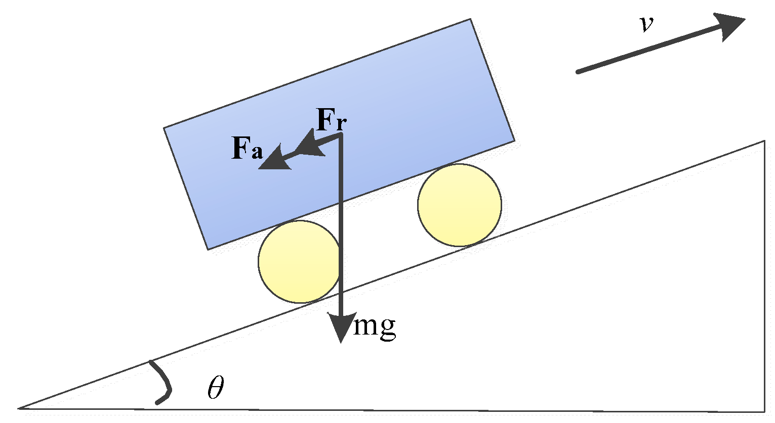
2.3. Energy Consumption Model
3. Path-Planning Algorithm Design
3.1. Description of the Problem
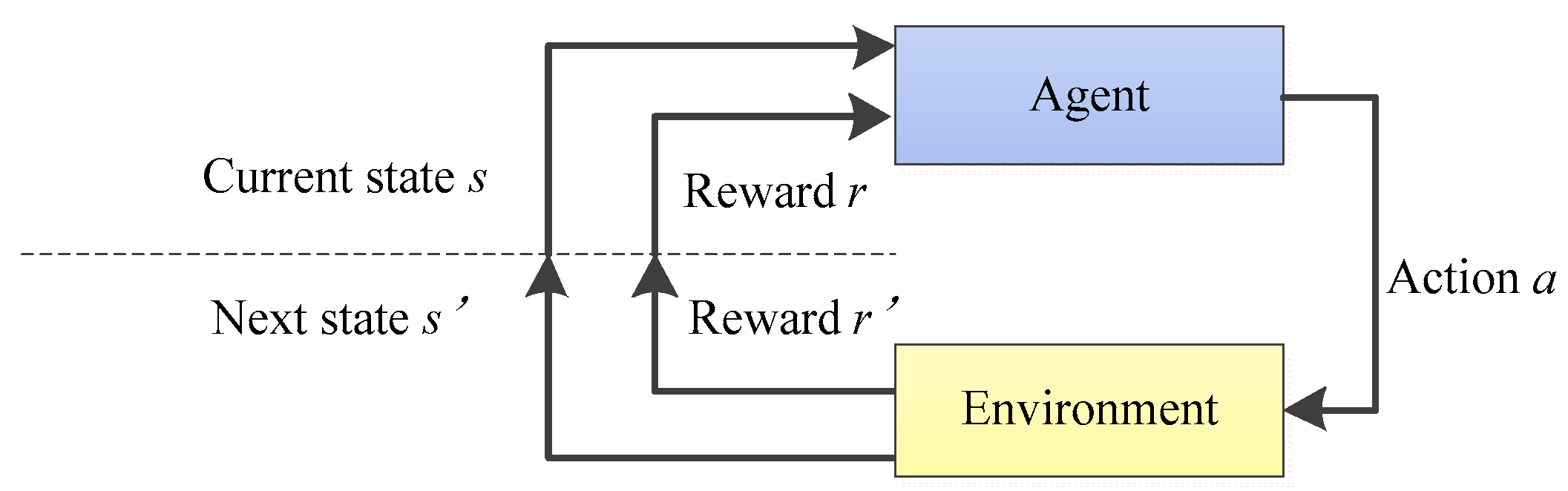
3.2. Principle of the DQN Algorithm
3.3. Design of A-DQN Algorithm Based on Heuristic Exploration
3.3.1. State Space
- Pose indicates the current position of the agent;
- Elevation represents the actual elevation value of each grid point;
- Goal indicates the location of the target point;
- Terrain is a static representation containing terrain-type labels (tterrain) at each grid point, classified by traversability. In this paper, the grass label is tterrain = 0 and the mud label is tterrain = 1:
3.3.2. Action Spaces and Reward Functions
3.3.3. Neural Network Architecture
3.3.4. Hybrid Exploration Strategy Based on A*
| Algorithm 1. A-DQN Algorithm pseudo-code |
| 1:Initialize environment env and agent 2: for i_episode in range 3: state, reward, done = env.reset() 4: while not done and env.steps_counter < max_step 5: training_strategy ⟵ select_training_strategy(i_episode) 6: if training_strategy = ‘A*’ then 7: action ⟵ select_action_by_A*(state) 8: else if training_strategy = ‘random’ then 9: action ⟵ select_action_random(state) 10: else 11: action ⟵ agent.take_action(state) 12: end if 13: next_state, reward, done ⟵ env.step(state,action) 14: replay_buffer.add(state, action, reward, next_state, done) 15: if replay_buffer.size ≥ minimal_size then 16: agent.update(reply_buffer.sample(batch_size)) 17: end if 18: end while 19: end for 20: save agent |
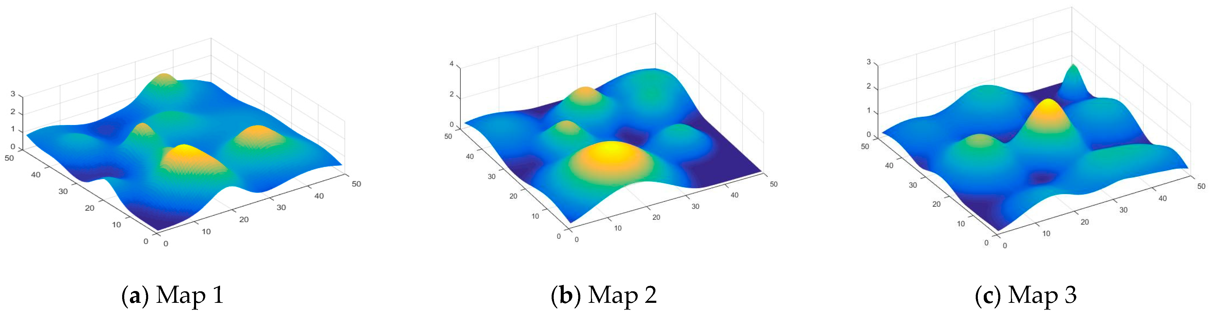
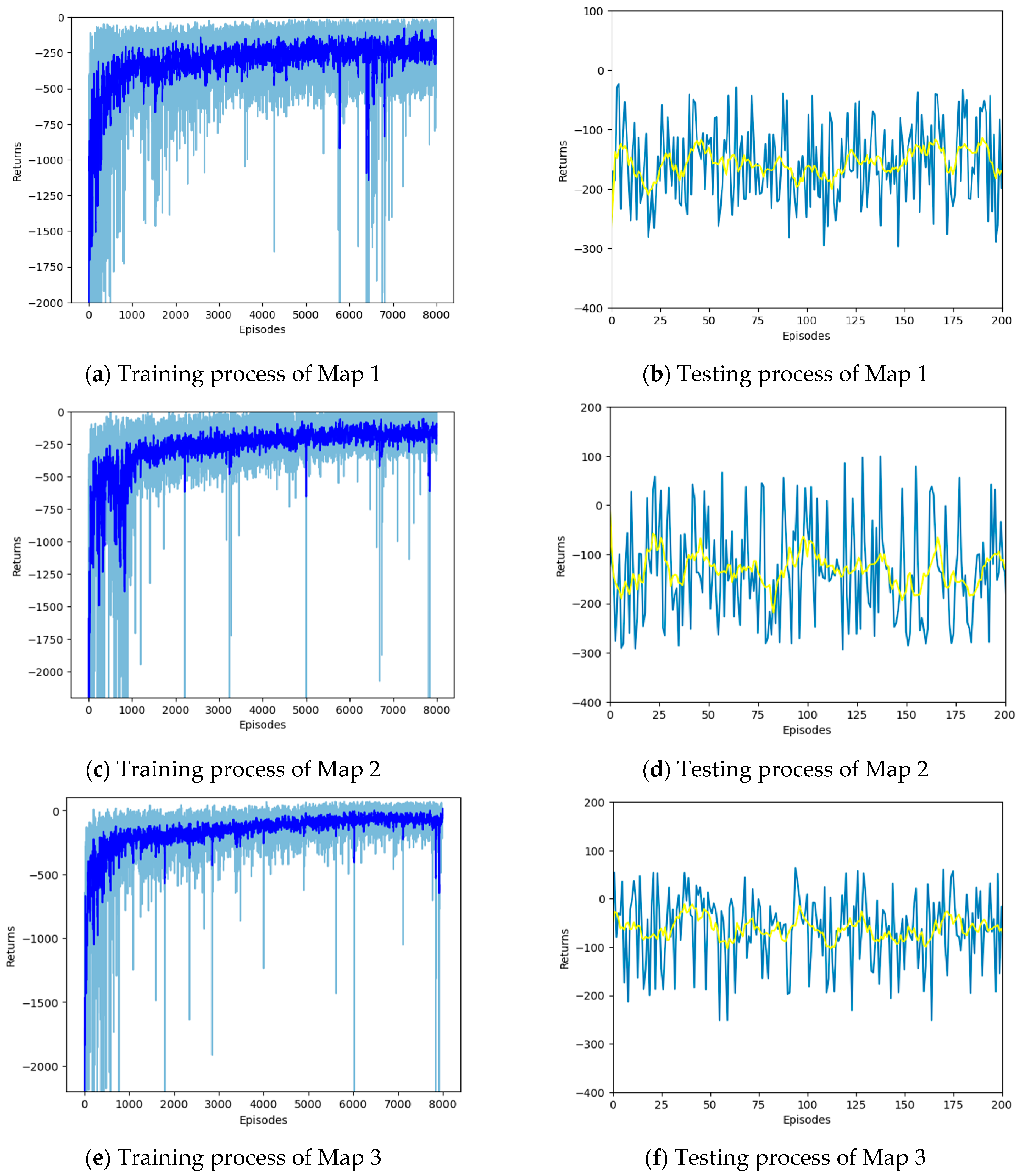
4. Simulation Experiment
4.1. Training Setup
4.2. Simulation Results and Analysis
5. Conclusions
Author Contributions
Funding
Institutional Review Board Statement
Informed Consent Statement
Data Availability Statement
Acknowledgments
Conflicts of Interest
References
- Ku, D.; Choi, M.; Oh, H.; Shin, S.; Lee, S. Assessment of the resilience of pedestrian roads based on image deep learning models. Proc. Inst. Civ. Eng. Munic. Eng. 2022, 175, 135–147. [Google Scholar] [CrossRef]
- Choi, M.J.; Ku, D.G.; Lee, S.J. Integrated YOLO and CNN algorithms for evaluating degree of walkway breakage. KSCE J. Civ. Eng. 2022, 26, 3570–3577. [Google Scholar] [CrossRef]
- Elassad, Z.E.A.; Mousannif, H. The application of machine learning techniques for driving behavior analysis: A conceptual framework and a systematic literature review. Eng. Appl. Artif. Intell. 2020, 87, 103312. [Google Scholar] [CrossRef]
- Qin, X.; Tang, J.; Liang, J.; Zhu, F. A comparative review on multi-modal sensors fusion based on deep learning. Signal Process. 2023, 213, 108550. [Google Scholar]
- Lee, H.; Kwon, J.; Kwon, C. Learning-based uncertainty-aware navigation in 3D off-road terrains. In Proceedings of the IEEE International Conference on Robotics and Automation (ICRA), London, UK, 29 May–2 June 2023; pp. 10061–10068. [Google Scholar]
- Garcia, F.; Martin, D.; De La Escalera, A.; Armingol, J.M. Sensor fusion methodology for vehicle detection. IEEE Intell. Transp. Syst. Mag. 2017, 9, 123–133. [Google Scholar] [CrossRef]
- Dijkstra, E.W. A note on two problems in connexion with graphs. Numer. Math. 1959, 1, 269–271. [Google Scholar] [CrossRef]
- Hart, P.E.; Nilsson, N.J.; Raphael, B. A formal basis for the heuristic determination of minimum cost paths. IEEE Trans. Syst. Sci. Cybern. 1972, 4, 100–107. [Google Scholar] [CrossRef]
- Bayili, S.; Polat, F. Limited-Damage A*: A path search algorithm that considers damage as a feasibility criterion. Knowl.-Based Syst. 2011, 24, 501–512. [Google Scholar] [CrossRef]
- Zhang, H.M.; Li, M.L.; Yang, L. Safe path planning of mobile robot based on improved A* algorithm in complex terrains. Algorithms 2018, 11, 44. [Google Scholar] [CrossRef]
- LaValle, S.M.; Kuffner, J.J. Rapidly-exploring random trees: Progress and prospects. Algorithmic Comput. Robot. 2001, 293, 303–307. [Google Scholar]
- Karaman, S.; Frazzoli, E. Sampling-based algorithms for optimal motion planning. Int. J. Robot. Res. 2011, 30, 846–894. [Google Scholar] [CrossRef]
- Jeong, I.B.; Lee, S.J.; Kim, J.H. Quick-RRT*: Triangular inequality-based implementation of RRT* with improved initial solution and convergence rate. Expert Syst. Appl. 2019, 123, 82–90. [Google Scholar] [CrossRef]
- Kavraki, L.E.; Svestka, P.; Latombe, J.C.; Overmars, M.H. Probabilistic roadmaps for path planning in high-dimensional configuration spaces. IEEE Trans. Robot. Autom. 1996, 12, 566–580. [Google Scholar]
- Vidana, J.I.S.; Motes, J.; Sandstrom, R.; Amato, N. Representation-optimal multi-robot motion planning using conflict-based search. IEEE Robot. Autom. Lett. 2021, 6, 4608–4615. [Google Scholar] [CrossRef]
- Reshamwala, A.; Vinchurkar, D.P. Robot path planning using an ant colony optimization approach: A survey. Int. J. Adv. Res. Artif. Intell. 2013, 2, 65–71. [Google Scholar]
- Suresh, K.S.; Venkatesan, R.; Venugopal, S. Mobile robot path planning using multi-objective genetic algorithm in industrial automation. Soft Comput. 2022, 26, 7387–7400. [Google Scholar] [CrossRef]
- Zhang, L.; Zhang, Y.; Li, Y. Mobile robot path planning based on improved localized particle swarm optimization. IEEE Sens. J. 2021, 21, 6962–6972. [Google Scholar] [CrossRef]
- Lv, T.; Feng, M. A smooth local path planning algorithm based on modified visibility graph. Mod. Phys. Lett. B 2017, 31, 1740091. [Google Scholar] [CrossRef]
- Ley-Rosas, J.J.; González-Jiménez, L.E.; Loukianov, A.G.; Ruiz-Duarte, J.E. Observer based sliding mode controller for vehicles with roll dynamics. J. Frankl. Inst. 2019, 356, 2559–2581. [Google Scholar] [CrossRef]
- Tian, H.; Li, B.; Huang, H.; Han, L. Driving risk-aversive motion planning in off-road environment. Expert Syst. Appl. 2023, 216, 119426. [Google Scholar] [CrossRef]
- Shen, C.; Yu, S.; Ersal, T. A three-phase framework for global path planning for nonholonomic autonomous vehicles on 3D terrains. IFAC-Pap. 2021, 54, 160–165. [Google Scholar] [CrossRef]
- Goulet, N.; Ayalew, B. Energy-optimal ground vehicle trajectory planning on deformable terrains. IFAC-Pap. 2022, 55, 196–201. [Google Scholar] [CrossRef]
- Zhang, H.; Zhang, Y.; Liu, C.; Zhang, Z. Energy efficient path planning for autonomous ground vehicles with Ackermann steering. Robot. Auton. Syst. 2023, 162, 106666. [Google Scholar] [CrossRef]
- Raja, R.; Dutta, A. Path Planning in Dynamic Environment for a Rover using A∗and Potential Field Method. In Proceedings of the 18th International Conference on Advanced Robotics (ICAR), Hong Kong, China, 10–12 July 2017; IEEE: Piscataway, NJ, USA, 2017; pp. 578–582. [Google Scholar]
- Hu, H.; Zhang, K.; Tan, A.H.; Ruan, M.; Nejat, G. Sim-to-real pipeline for deep reinforcement learning for autonomous robot navigation in cluttered rough terrain. IEEE Robot. Autom. Lett. 2021, 6, 6569–6576. [Google Scholar] [CrossRef]
- Josef, S.; Degani, A. Deep reinforcement learning for safe local planning of a ground vehicle in unknown rough terrain. IEEE Robot. Autom. Lett. 2020, 5, 6748–6755. [Google Scholar] [CrossRef]
- Chavez-Garcia, R.O.; Guzzi, J.; Gambardella, L.M.; Giusti, A. Learning ground traversability from simulations. IEEE Robot. Autom. Lett. 2018, 3, 1695–1702. [Google Scholar] [CrossRef]
- Wulfmeier, M.; Rao, D.; Wang, D.Z. Large-scale cost function learning for path planning using deep inverse reinforcement learning. Int. J. Robot. Res. 2017, 36, 1073–1087. [Google Scholar] [CrossRef]
- Zhang, K.; Niroui, F.; Ficocelli, M. Robot navigation of environments with unknown rough terrain using deep reinforcement learning. In Proceedings of the 2018 IEEE International Symposium on Safety, Security, and Rescue Robotics (SSRR), Philadelphia, PA, USA, 6–8 August 2018; IEEE: Piscataway, NJ, USA, 2018; pp. 1–7. [Google Scholar]
- Mnih, V. Playing Atari with deep reinforcement learning. arXiv 2013, arXiv:1312.5602. [Google Scholar]


| Parameter | Meaning | Value |
|---|---|---|
| γ | Attenuation factor | 0.99 |
| Learning_rate | Learning rate | 0.0001 |
| Episodes | Number of training rounds | 8000 |
| Replay_memory | Memory pool size | 20,000 |
| Max_step | Maximum number of steps per episodes | 150 |
| Batch_size | Batch size of memory replay | 64 |
| k1 | Slope penalty intensity factor | 4 |
| k2 | Terrain penalty intensity factor | 10 |
| Map | Algorithm | Mean Distance (m) | Mean Energy (u) | Sum | Mean Time (s) |
|---|---|---|---|---|---|
| Map 1 | A-DQN | 3717.2798 ± 282.39 | 11,223.2752 ± 3392.35 | 14,940.5550 | 0.23 ± 0.04 |
| Dijkstra | 4113.0482 ± 257.26 | 11,093.0519 ± 3392.44 | 15,206.1001 | 87.79 ± 0.07 | |
| A* | 4109.1041 ± 223.35 | 11,099.4611 ± 3376.78 | 15,208.5652 | 56.08 ± 1.64 | |
| RRT | 5255.3713 ± 427.61 | 23,606.0725 ± 3528.53 | 28,861.4438 | 201.41 ± 258.18 | |
| Map 2 | A-DQN | 4139.8562 ± 331.12 | 11,934.2752 ± 3476.42 | 16,074.1314 | 0.23 ± 0.07 |
| Dijkstra | 4451.9524 ± 278.43 | 11,785.6741 ± 3295.34 | 16,237.6265 | 102.12 ± 0.24 | |
| A* | 4452.0589 ± 245.31 | 11,788.0265 ± 3338.57 | 11,230.0854 | 65.66 ± 3.06 | |
| RRT | 4923.7144 ± 400.08 | 22,933.5654 ± 3427.93 | 27,857.2798 | 242.03 ± 307.56 | |
| Map 3 | A-DQN | 3956.2568 ± 301.13 | 11,697.7548 ± 3428.97 | 15,654.0116 | 0.22 ± 0.03 |
| Dijkstra | 4248.2987 ± 265.70 | 11,516.4835 ± 3219.78 | 15,764.7822 | 97.12 ± 0.03 | |
| A* | 4249.9691 ± 230.60 | 11,521.2658 ± 3262.39 | 115,771.2349 | 54.30 ± 1.09 | |
| RRT | 4863.5697 ± 395.15 | 20,514.6567 ± 3065.51 | 25,378.2264 | 209.85 ± 248.27 |
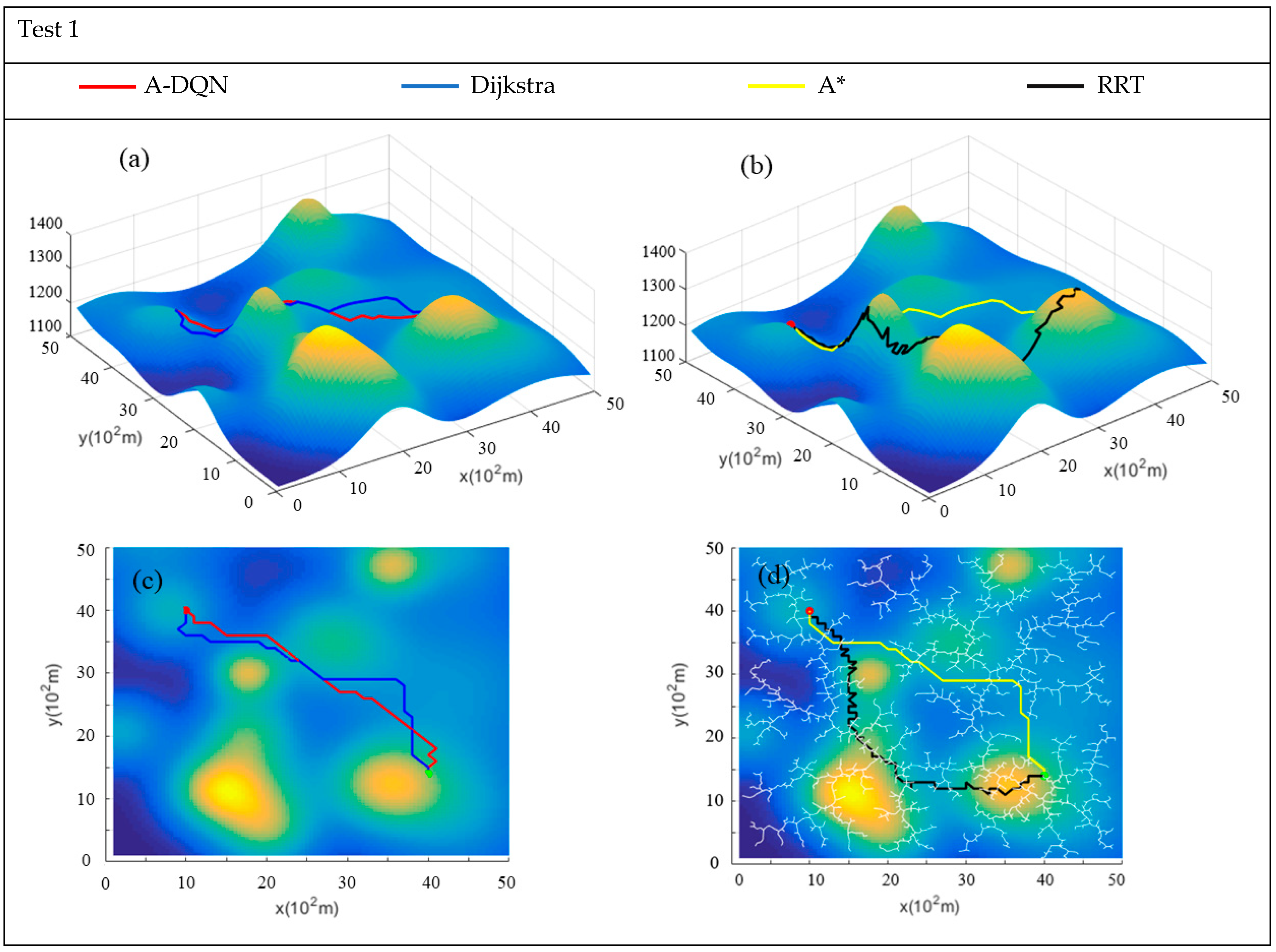
| Test 1 | ||||
|---|---|---|---|---|
| Arithmetic | Distance (m) | Energy (u) | Sum | Time (s) |
| A-DQN | 4607.9942 | 10,140.0362 | 1.4748 × 10⁴ | 0.22 |
| Dijkstra | 5050.3762 | 10,020.6006 | 1.5071 × 10⁴ | 197.63 |
| A* | 4850.982 | 10,046.57526 | 1.4898 × 10⁴ | 167.94 |
| RRT | 5255.3713 | 25,210.7808 | 3.0466 × 10⁴ | 213.69 |
| Test 2 | ||||
|---|---|---|---|---|
| Arithmetic | Distance (m) | Energy (u) | Sum | Time (s) |
| A-DQN | 4518.2799 | 15,580.0503 | 2.0098 × 10⁴ | 0.23 |
| Dijkstra | 4868.6638 | 15,319.1458 | 2.0188 × 10⁴ | 85.72 |
| A* | 4868.6638 | 15,319.1458 | 2.0188 × 10⁴ | 42.67 |
| RRT | 6050.9644 | 30,981.1138 | 3.7032 × 10⁴ | 158.12 |
| Test 3 | ||||
|---|---|---|---|---|
| Arithmetic | Distance (m) | Energy (u) | Sum | Time (s) |
| A-DQN | 4293.9799 | 10,076.9074 | 1.4371 × 10⁴ | 0.22 |
| Dijkstra | 4434.5732 | 10,014.551 | 1.4449 × 10⁴ | 63.60 |
| A* | 4434.5732 | 10,014.551 | 1.4449 × 10⁴ | 29.19 |
| RRT | 4426.41 | 21,454.6406 | 2.5881 × 10⁴ | 199.36 |
Disclaimer/Publisher’s Note: The statements, opinions and data contained in all publications are solely those of the individual author(s) and contributor(s) and not of MDPI and/or the editor(s). MDPI and/or the editor(s) disclaim responsibility for any injury to people or property resulting from any ideas, methods, instructions or products referred to in the content. |
© 2025 by the authors. Licensee MDPI, Basel, Switzerland. This article is an open access article distributed under the terms and conditions of the Creative Commons Attribution (CC BY) license (https://creativecommons.org/licenses/by/4.0/).
Share and Cite
Yang, Y.; Zhang, Z. Rough-Terrain Path Planning Based on Deep Reinforcement Learning. Appl. Sci. 2025, 15, 6226. https://doi.org/10.3390/app15116226
Yang Y, Zhang Z. Rough-Terrain Path Planning Based on Deep Reinforcement Learning. Applied Sciences. 2025; 15(11):6226. https://doi.org/10.3390/app15116226
Chicago/Turabian StyleYang, Yufeng, and Zijie Zhang. 2025. "Rough-Terrain Path Planning Based on Deep Reinforcement Learning" Applied Sciences 15, no. 11: 6226. https://doi.org/10.3390/app15116226
APA StyleYang, Y., & Zhang, Z. (2025). Rough-Terrain Path Planning Based on Deep Reinforcement Learning. Applied Sciences, 15(11), 6226. https://doi.org/10.3390/app15116226