Evaluation of Feature Selection and Regression Models to Predict Biomass of Sweet Basil by Using Drone and Satellite Imagery

Abstract

The integration of precision agriculture technologies, such as remote sensing through drones and satellites, has significantly enhanced real-time crop monitoring. This study is among the first to combine multispectral data from both a drone equipped with Altum-PT camera and PlanetScope satellite imagery to predict fresh biomass in sweet basil grown in an open field, demonstrating the added value of integrating different spatial scales. A dataset of 40 sampling points was built by combining remote sensing data with field measurements, and seven vegetation indices were calculated for each point. Feature selection was performed using three different methods (F-score, Recursive Feature Elimination, and model-based selection), and the most informative features were then processed through Principal Component Analysis. Eight regression models were trained and evaluated using leave-one-out cross-validation. The best-performing models were Random Forest (R² = 0.96 in training, R² = 0.65 in testing) and k-Nearest Neighbours (R² = 0.74 in training, R² = 0.94 in testing), with kNN demonstrating superior generalization capability on unseen data. These findings highlight the potential of combining drone and satellite imagery for modelling basil agronomic traits, offering valuable insights for optimizing crop management strategies.

1. Introduction

Sweet basil (Ocimum basilicum L.) is an aromatic herbaceous crop belonging to the Lamiaceae family. The genus Ocimum has around 30 aromatic species, both herbaceous and shrubs, and both annual and perennial, native to Asia, central–southern America and Africa [1,2]. This genus is featured by a high variability at the morphological, chemical and genetic levels due to cross-pollination [3,4]. Thanks to its aroma and flavour, sweet basil is a cherished herb in various culinary traditions around the world but is also used for medical purposes and as an insect-controlling agent [3,5]. It is characterized by high economic interest [6].

In the “Guide to Plant Identification”, the authors describe basil as an annual herbaceous plant that reaches a height of 20–40 cm [7]. The stem is erect with a quadrangular section and tends to become woody at the base. Leaves are petiolate with ovate–lanceolate lamina that are entire or sparsely serrated, and glabrous, measuring 2–5 cm in length. Its colour varies from pale green to intense green or purple in some varieties. Leaves are the main commercial part of interest of the plant. The flowers, small and white, have a corolla with five irregular petals and are grouped in inflorescences at the axil of the leaves. The flowers are hermaphrodite, and the pollination is entomophilous; flowering takes place from June to October. The fruit is a tetrachenium from which four small oval dark brown achenes derive, detaching at maturity.

Sweet basil is one of the most widely cultivated and distributed aromatic plants globally. In Italy, the cultivated area of basil reached approximately 290 hectares in 2024 [8]. This growth trend was driven by the rising demand from the food industry. Basil cultivation is particularly concentrated in four Italian regions: Lombardia, Emilia-Romagna, Marche, and Campania [9]. To improve basil production, precision agriculture integrated with innovative data analysis techniques is a promising solution.

In recent years, the introduction of precision agriculture technologies has improved crop management, promoting greater economic, social, and environmental sustainability [10]. Remote sensing is a key technique in precision agriculture and allows for the precise monitoring of crop conditions. Among the most promising technologies, drones equipped with spectral sensors have proven to be effective tools for collecting detailed data on plant health and vegetation indices. An interesting point is that visible spectral sensors are suitable for the analysis and quantification of important plant properties such as phenolic compounds and flavonoids [11]. Another study focuses on the discrimination of basil from similar plants using chlorophyll fluorescence imaging techniques, with great results obtained [12].

Machine learning and deep learning techniques can be employed for the precise, real-time detection and classification of basil diseases, with the goal of improving agricultural productivity, reducing labour and costs, and increasing diagnostic accuracy [13]. For example, Son et al. compared three linear classifiers and five non-linear classifiers to identify the optimal model for stress classification [14], while another study employed a Convolutional Neural Network to detect drought stress, achieving an accuracy of 96.9% [15].

Considering the overall state of research on sweet basil, there is very little attention dedicated to field-based studies, with most research focused on stress detection and growth monitoring under controlled environments. To date, no scientific investigations have explored the application of remote sensing combined with machine learning algorithms to predict basil biomass under open-field conditions. This represents a critical knowledge gap, especially given the growing relevance of precision agriculture technologies in optimizing crop management and sustainability for specialty crops.

Addressing this gap, the current work aims to evaluate and compare the performance of eight regression models trained to predict the fresh biomass of sweet basil. Images are acquired through two different remote sensing techniques: a drone equipped with a multispectral–thermal sensor and the PlanetScope satellite. Vegetation indices were extracted and analyzed to identify the most predictive features. Lastly, the predictive models were then trained and assessed to determine their effectiveness in estimating biomass.

The central research question is whether the integration of drone and satellite imagery, combined with machine learning algorithms, can enable the accurate and generalizable prediction of sweet basil biomass under open-field conditions. By combining advanced remote sensing technologies with machine learning approaches, this study demonstrates a novel methodology for the real-time, non-destructive biomass estimation of sweet basil in open-field cultivation. The outcomes not only provide valuable insights into the potential of precision agriculture tools for minor crops but also lay the groundwork for future large-scale applications aimed at enhancing yield prediction, resource management, and overall farm productivity.

2. Materials and Methods

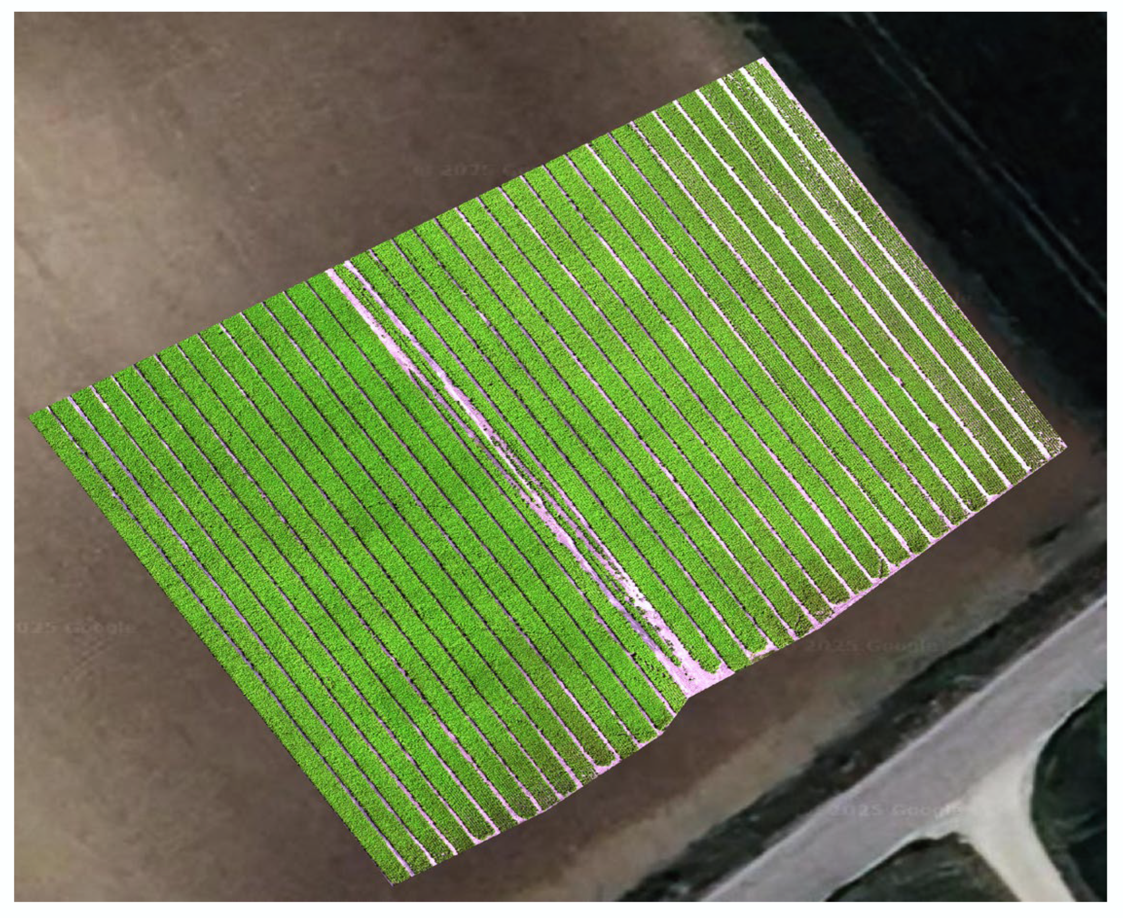
Experimental activities were conducted at an organic farm in central Italy. The field considered for the experimentation has a total area of 9.21 hectares. Specifically, the sampled area covers approximately 0.3 hectares and is in the southeast part of the entire plot (Figure 1). The soil involved in the case study is characterized by a medium-textured structure. The organic matter content is approximately 1.8%. The level of available phosphorus is low, while the level of exchangeable potassium is high.

Basil was cultivated in succession to parsley. The chosen variety is Noga F1 from the seed company Fenix, which is a basil hybrid resistant to downy mildew, distinguished by its characteristic spoon-shaped leaves, typical of Genoese basil. The crop was seeded on 6 May 2024, using a mechanical row seeder. The working width of the machine is 150 cm, with an inter-row spacing of approximately 18 cm, resulting in a total of 8 rows of basil within the working width. The distance between rows is 20 cm. The seeding density is 8.5 kg/ha. Basil is harvested in multiple cuttings throughout the season, and the subdivision of the harvesting area is determined based on market demand. Weed control is carried out through hoeing during the early growth stages, followed by manual weeding before each cutting.

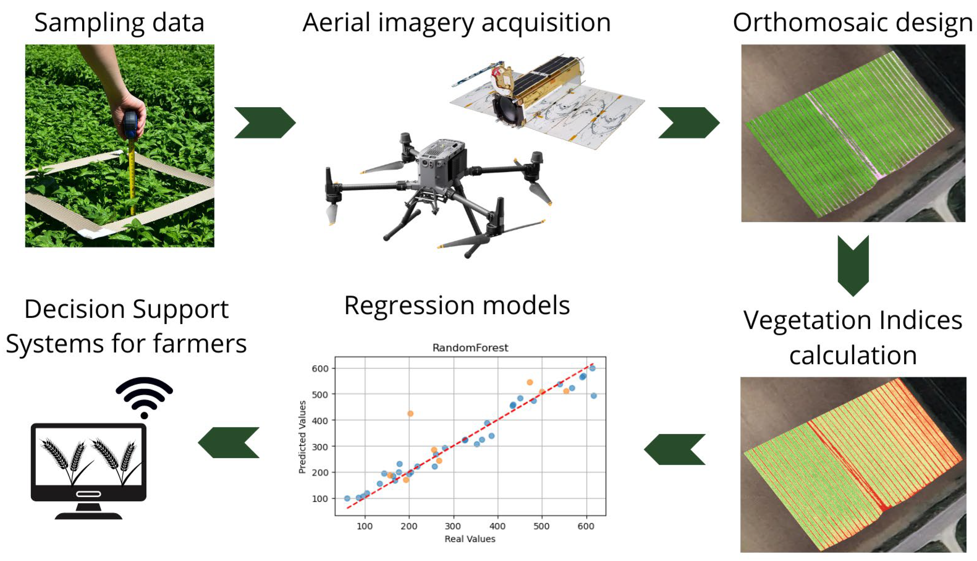
The following paragraphs describe the entire workflow, from data acquisition to model evaluation. Figure 2 is useful for summarizing and improving the understanding of the workflow.

2.1. Plant Sampling Data

Sampling of basil took place over two consecutive days (8–9 August 2024). Within the area, ten rows of basil were sampled, and for each row, four sampling points were collected, totalling 40 samples. Each sample is approximately 10 m apart. For each sampling point, GPS coordinates were recorded using a mobile device. Although the positional accuracy of the smartphone GPS is lower compared to that of professional surveying instruments, it was sufficient for the purpose of sample georeferencing, given the spatial separation between points. No high-precision differential correction was applied, as the required spatial resolution was compatible with the scale of sampling and remote sensing analysis performed. Additionally, height and biomass were measured.

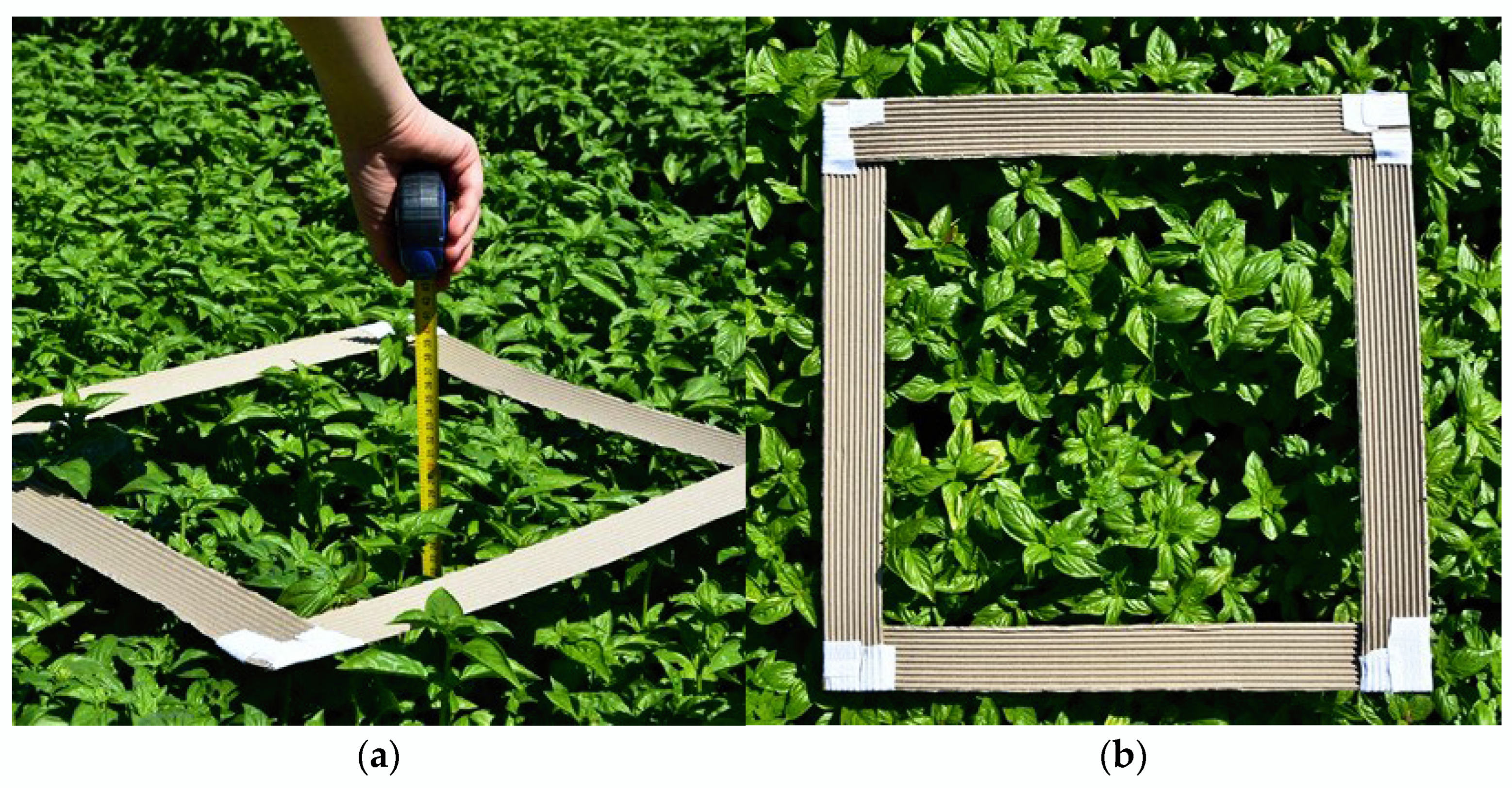
Sampling started on 8 August 2024. The tools used for each measurement included a wheel metre (Figure 3a), a mobile device for GPS positioning, and a cardboard frame measuring 50 cm × 50 cm in size (Figure 3b). The protocol involves the following steps: We positioned the frame above the plants in the row to define a surface area of 0.25 m². Then, we selected three random plants to measure their height in centimetres. The day after, the sampling consisted of collecting the biomass of basil plants from the sampling points established before thanks to GPS coordinates. Once positioned at the same points, the frame was placed, and the biomass of the basil plants within the 0.25 m² area was obtained manually. Cutting was performed using a knife blade, and the yield from each sampling point was collected in a plastic bag, numbered with the progressive sample reference. The cutting process aimed to replicate the mechanical harvesting typically performed by industrial harvesters for aromatic plants, which is why the cut was made approximately 4–6 cm above the cutting point from the previous harvest. Subsequently, the samples were weighed individually.

2.2. Drone Survey

The survey utilized the Matrice 350 RTK drone (Shenzhen DJI Sciences and Technologies Ltd., Shenzhen, China). The drone is equipped with the Altum-PT camera (MicaSense^®, AgEagle Aerial Systems Inc., Wichita, KS, USA), which is a multispectral, panchromatic, and thermal sensor. The central wavelengths and bandwidths of each band are reported in

Table 1. Central wavelengths and bandwidths of Altum-PT camera.

Band	Central Wavelengths	Bandwidths
Blue	457 nm	32 nm
Green	560 nm	27 nm
Red	668 nm	16 nm
Red Edge	717 nm	12 nm
Near-Infrared	842 nm	57 nm
Panchromatic	634.5 nm	463 nm
Long-Wave Infrared	10.5 μm	6 μm

.

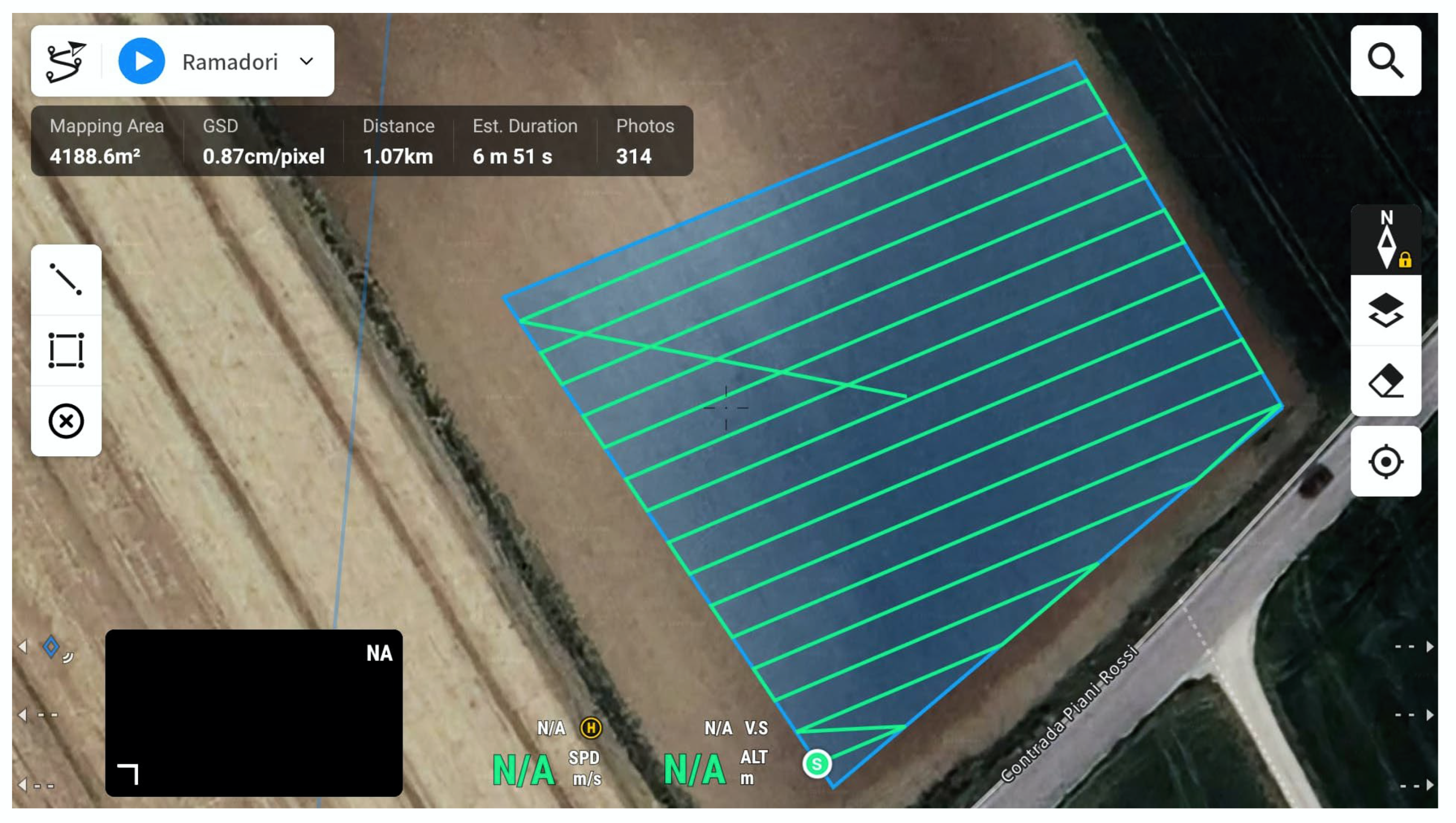
On 8 August 2024, a sweet basil survey was conducted using the drone. The mission of the flight consisted of two steps: calibrating the camera through the calibration panel and mapping the sampled area to acquire the spectral bands (Figure 4). The navigation path was set, and image acquisition by the sensor for each band was planned. The specific flight characteristics are reported in

Table 2. Flight parameters.

Parameter	Value
Altitude	20 m
Speed	2 m/s
Ground resolution	0.87 cm/pixel
Frontal overlap	75%
Side overlap	75%

. The flight took place in the morning, between 11:00 AM and 12:00 PM. Weather conditions were suitable for flying, as it was a sunny day with no clouds, calm winds, and good temperatures.

2.3. Satellite Images

PlanetScope is a satellite constellation operated by Planet Labs, designed for high-frequency Earth observation. Each PlanetScope satellite, known as Dove, is equipped with a multispectral sensor capturing imagery in the coastal blue, blue, green I, green, yellow, red, red edge, and near-infrared bands (

Table 3. Band composition and relative wavelength of PlanetScope satellite.

Band	Wavelengths
Costal Blue	431–452 nm
Blue	465–515 nm
Green I	513–549 nm
Green	547–583 nm
Yellow	600–620 nm
Red	650–680 nm
Red Edge	697–713 nm
Near-Infrared	845–885 nm

). With a spatial resolution of approximately 3 m per pixel, PlanetScope provides daily global coverage, enabling applications in precision agriculture.

2.4. Images Pre-Processing

For image pre-processing, Pix4D Mapper^® (Pix4D SA, Prilly, Switzerland) was used as a photogrammetric processing software for drone mapping. The 2D output that this programme can generate is the orthomosaic, which is a composition of geometrically corrected and georeferenced frames.

All images acquired by the Altum-PT sensor during the drone flight, as well as images obtained during the initial and final calibration of the sensor, are uploaded to the software. Desired image processing options are set, and the geographic reference system is specified. The programme can automatically generate an orthomosaic for each spectral band captured by the sensor.

2.5. Image Processing

QGis (3.34.9 version) is an open-source geographic information system used for image analysis. The orthomosaic for each spectral band was imported as a raster file. Using a mask generated to delineate the boundaries of the area of interest, the raster was cropped. Next, a .csv file containing the geographic coordinates (latitude and longitude) of each sampling point, along with information regarding the average heights recorded and the biomass of each sample, was imported.

Three different buffers were created around each sampling point at distances of 30, 45, and 60 cm. At this stage, seven vegetation indices were calculated: the Normalized Difference Vegetation Index (NDVI), the Green NDVI (GNDVI), the Normalized Difference Red Edge (NDRE), the Chlorophyll Vegetation Index (CVI), the Enhanced Vegetation Index (EVI), the Soil-Adjusted Vegetation Index (SAVI), and a thermal index (TI). Formulas are included in

Table 4. Vegetation indices formulas and references.

Index	Formula	Reference
NDVI	${\displaystyle \frac{NIR-R}{NIR+R}}$	[16]
GNDVI	${\displaystyle \frac{NIR-G}{NIR+G}}$	[17]
NDRE	${\displaystyle \frac{NIR-RE}{NIR+RE}}$	[18]
CVI	${\displaystyle \frac{NIR\times Red}{G^2}}$	[19]
EVI 1	$G\times {\displaystyle \frac{NIR-R}{\left(NIR+C1\times R-C2\times B+L\right)}}$	[20]
SAVI 2	${\displaystyle \frac{NIR-R}{NIR+R+L}}\times \left(1+L\right)$	[21]
TI	${\displaystyle \frac{LWIR}{100}}-273.15$	Pix4D Documentation

¹ G = 2.5 is the gain factor, L = 1 is the canopy background adjustment that addresses non-linear, differential NIR and red radiant transfer through the canopy; C1 = 6 and C2 = 7.5 are the coefficients of the aerosol resistance term, which uses the blue band to correct for aerosol influences in the red band. ² L is a correction factor set to 1 for very low vegetation density, 0.5 for intermediate density (the one chosen in the current case study), and 0.25 for high density.

. Finally, zonal statistics for each vegetation index were calculated at the sampling points. This tool computes the mean value of the raster pixels within the buffer area of each sampling point. All these values were then exported into .xlsx format for both drone and satellite images.

2.6. Data Analysis

The full dataset consists of 40 rows, 1 for each sampling point, and 42 columns (Appendix A). For each of them, fresh biomass (“BIO”) information is collected and called the target variable. Vegetation indices are integrated with agronomic parameters and represent the predictive variables.

The pipeline described in the following paragraphs was processed, coding the algorithm in the Python (3.12.7 version) programming language. The main libraries used include Pandas (2.2.2 version), Matplotlib (3.9.2 version), NumPy (1.26.4 version), and Scikit-learn (1.5.1 version).

Three independent feature selection techniques were applied to identify the most informative variables. The features retained were those consistently ranked higher in at least two methods. To further reduce redundancy and mitigate multicollinearity, Principal Component Analysis (PCA) was performed on the selected features. The first three principal components were used as predictors in the regression models. This transformation ensured that the input variables were uncorrelated. Then, the pipeline involved robust scaling using Robust Scaler and an exhaustive hyperparameter search using leave-one-out cross-validation to ensure a reliable and unbiased evaluation of various regression models. For each regressor, the search space was defined (

Table 5. For each model, the following search spaces weretested.

Model	Search Space
Linear Regression	{}
Ridge Regression	alpha: [0.1, 1, 10, 100]
Lasso Regression	alpha: [0.01, 0.1, 1, 10]
Random Forest	n_estimators: [50, 100, 200] max_depth: [None, 10, 20]
Gradient Boosting	n_estimators: [50, 100, 200] learning_rate: [0.01, 0.1, 0.2]
Support Vector Regression	C: [0.1, 1, 10] kernel: [linear, rbf]
Decision Tree	max_depth: [None, 10, 20, 30] min_samples_split: [2, 5, 10] min_samples_leaf: [1, 5, 10]
k-Nearest Neighbours	n_neighbors: [3, 5, 7, 10]

). By visualizing both training and test predictions along with performance metrics, this approach not only identifies the best-performing model but also provides insights into its generalization capacity, which is crucial for non-destructive biomass estimation. For each model, the best combination of hyperparameters was selected based on the minimum Mean Absolute Error (MAE) value obtained during the leave-one-out cross-validation.

2.7. Features Selection

In order to identify the most informative features and to reduce complexity for improving performance [22], three different features selection techniques were applied: F-Score, Recursive Feature Elimination (RFE) and model-based selection.

The feature selection method based on the F-Score seeks to determine which independent variables have the greatest ability to explain variability in the target [23,24,25,26]. Variables with a high F-Score are those that are most strongly related to the target, while those with a low F-Score may not have a significant relationship and may be excluded from the model. In addition, the p-Value measures the statistical significance of the F test. A low p-Value (less than 0.05 for this work) indicates that the characteristic has a significant correlation with the target, suggesting that it is important in the model.

The RFE method aims to identify the most important variables for the model, by recursively removing those that are least significant [27,28,29]. RFE is particularly useful for improving the accuracy of a model by reducing the dimensionality of the dataset. Once the model is trained, RFE ranks each feature based on a metric that depends on the type of model used. In the case of Linear Regression, the importance of a feature can be determined by its coefficients.

Model-based selection is another feature selection approach that exploits the ability of a model to calculate the importance of features during model training [30,31,32]. In the current work, the selected model is Random Forest. Once the Random Forest is trained, each tree in the model calculates how much each feature contributes to the final prediction. The importance of a feature is generally calculated using the decrease in purity of each tree node during its construction.

After applying the feature selection techniques, only the features that were considered important by at least two feature selection methods were chosen. For this reason, a top ten list was drawn up. To obtain the best regression performance, PCA (Principal Component Analysis) was performed on the best selected features.

PCA, also known as Karhunen–Loeve expansion, is the oldest multivariate technique developed before the Second World War. PCA is a classical feature extraction and data representation technique [33,34]. It analyzes a dataset that represents variations described by different dependent variables, which are generally interrelated [35,36,37]. Its purpose is to extract important information from the matrix and express this information as a set of new orthogonal variables called principal components. The correlation between a principal component and a variable quantifies the extent of shared information. Within the PCA framework, this correlation is referred to as a loading (or score). Notably, the sum of the squared correlation coefficients between a given variable and all principal components equals 1. Consequently, squared loadings offer a more intuitive interpretation than raw loadings, as they represent the proportion of the variable’s variance explained by the components.

2.8. Regression Models

Eight regression models were trained to predict fresh biomass: Linear Regression (LR), Ridge Regression, Least Absolute Shrinkage and Selection Operator (LASSO) Regression, Support Vector Regression (SVR), Decision Tree (DT), Random Forest (RF), Gradient Boosting (GB), and k-Nearest Neighbours (kNN).

LR is one of the simplest and most widely used methods for assessing the relationship between predictive variables and targets. This technique assumes that the relation is linear, and consequently, a change in one variable corresponds to a proportional change in the other [38,39]. Being a simple method, Linear Regression is often the preferred method for analyzing small datasets, and its results are also relatively easy to interpret. However, this approach may become ineffective when there are many predictive variables because the model has difficulty managing complexity or a situation in which the relationship between predictive and target variables is strongly non-linear.

Ridge Regression is used to address multicollinearity, high correlation between predictor variables, and overfitting in Linear Regression models [40]. It is a form of regularized regression that adds a penalty term to the loss function to constrain or regularize the coefficients of the model, making them smaller and more stable [41].

LASSO aims to identify the variables and corresponding regression coefficients, leading to a model that minimizes the prediction error [42,43,44]. This is achieved by imposing a constraint on the model parameters, which “shrink” the regression coefficients towards zero. Variables with a regression coefficient of zero after shrinkage are excluded from the model.

SVR is employed to identify a function that best represents the relationship between input features and the target variable [10]. It is a machine learning technique focused on learning the importance of each feature in capturing the relationship between inputs and outputs [45]. SVR achieves this by mapping the original non-linear input space into a higher-dimensional feature space through the use of a kernel function [46]. This transformation enables the handling of non-linear relationships, with the resulting feature space, represented by the kernel matrix, being utilized to solve the regression task.

DT is a powerful machine learning algorithm for identifying relevant features and uncovering patterns in large datasets, making it valuable for both classification and predictive modelling [47,48,49]. DT iteratively divides a dataset based on decision rules, selecting the feature that best separates the data. Each subdivision reduces the impurity and creates internal nodes until the stop criteria are met, with the final nodes containing the predictions [50]. Its ability to provide clear and interpretable decision rules has contributed to its widespread use in exploratory data analysis and predictive analytics for over twenty years.

RF is a robust regression method that leverages an ensemble of Decision Trees [51]. For each input, the predictions from the individual trees are aggregated to produce a final output [52]. To enhance the diversity of the trees and reduce their correlation, RF employs bagging, a technique that generates distinct subsets of the data for training each tree. This approach effectively boosts both the model’s robustness and predictive accuracy [53].

GB is an ensemble learning technique applicable to both regression and classification tasks [54]. It constructs a model iteratively by sequentially fitting weak learners and combining their predictions. The underlying principle of boosting is that it incrementally refines the model by considering all features in each iteration, thereby learning a functional mapping for each feature in the process [55].

The kNN algorithm is a non-parametric method that estimates the output for a given input based on the average value of its closest neighbours [10,56]. The training dataset consists of pairs of input and output values, and once trained, the model makes predictions for unseen instances by leveraging the values of nearby points [57]. A critical aspect of kNN is the selection of the hyperparameter K, which determines the number of neighbours considered. Choosing an excessively small K may lead to overfitting, as the model captures noise in the training data, whereas a large K can result in underfitting, reducing the model’s ability to capture local patterns in the data [58,59].

2.9. Evaluation Metrics

The most common evaluation metrics for regression models are R-Squared (R²), Mean Absolute Error (MAE), Mean Squared Error (MSE), and Root Mean Squared Error (RMSE). These metrics are properly described in the scientific literature [60,61]. According to Chicco et al., in the following formulas, X_i is the predicted ith value, and the Y_i element is the actual ith value.

R² is the coefficient of determination. It measures the proportion of variance in the dependent variable that is explained by the independent variables in a regression model. It ranges from 0 to 1, where higher values indicate a better fit. However, a high R² does not necessarily imply a well-performing model, especially in the presence of overfitting or multicollinearity.

$$R^2=1-{\displaystyle \frac{{\sum }_{i=1}^m{\left(X_i-Y_i\right)}^2}{{\sum }_{i=1}^m{\left(\overline{Y}-Y_i\right)}^2}}$$

MAE provides the average of the absolute difference between predicted and actual values, without considering their direction. It provides an intuitive measure of model accuracy by averaging the absolute differences, making it less sensitive to large outliers compared to squared error metrics.

$$MAE={\displaystyle \frac{1}{m}}·\sum _{i=1}^m\left|X_i-Y_i\right|$$

MSE calculates the average squared differences between predicted and actual values. By squaring the errors, it penalizes larger deviations more heavily, making it useful for emphasizing substantial prediction errors. The MSE is always a positive value.

$$MSE={\displaystyle \frac{1}{m}}·\sum _{i=1}^m{\left(X_i-Y_i\right)}^2$$

RMSE provides a balanced measure of model accuracy by accounting for both an average error magnitude and the impact of larger errors, making it particularly useful for comparing different models.

$$RMSE=\sqrt{{\displaystyle \frac{1}{m}}·\sum _{i=1}^m{\left(X_i-Y_i\right)}^2}$$

3. Results

Features that are considered important by at least two feature selection methods have been selected. The top ten features for each technique are reported in

Table 6. Top ten features selected through three feature selection techniques.

F-Score	RFE	RF-Based Selection
stat_gndvi_D45	stat_ndvi_S30	stat_ndvi_D60
stat_gndvi_D60	stat_ndvi_S45	stat_ndvi_D45
stat_ndvi_D60	stat_ndvi_S60	stat_ndvi_D30
stat_gndvi_D30	stat_gndvi_S30	stat_ndre_D60
stat_ndre_D45	stat_gndvi_S45	stat_cvi_D60
stat_ndvi_D45	stat_gndvi_S60	stat_ndre_D45
stat_ndre_D60	stat_ndre_S45	stat_evi_D30
stat_ndre_D30	stat_ndre_S60	stat_cvi_D45
stat_gndvi_S60	stat_savi_S30	stat_gndvi_D30
stat_ndre_S60	stat_savi_S60	stat_gndvi_D45

.

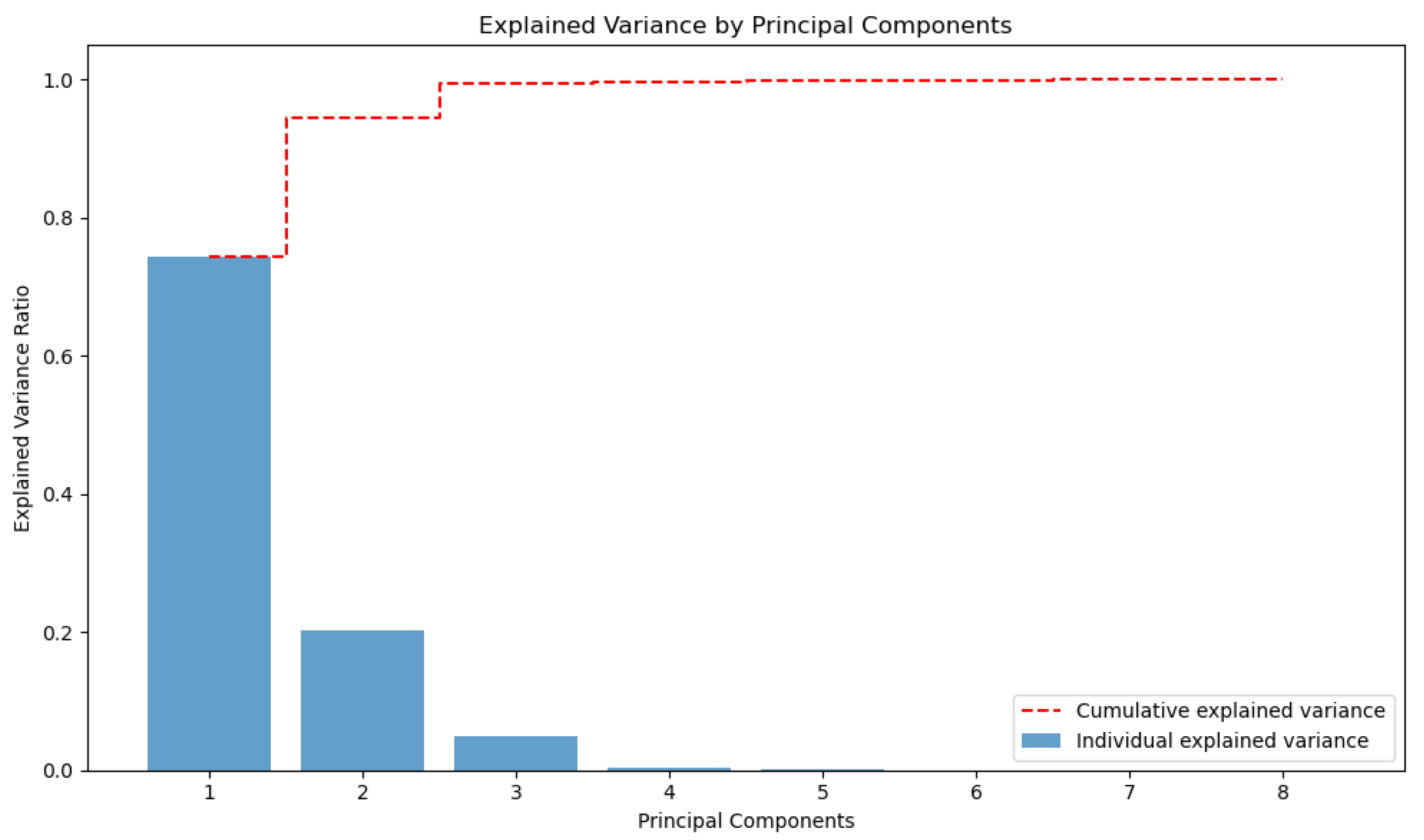
The selected features are stat_gndvi_D45, stat_gndvi_D30, stat_gndvi_S60, stat_ndvi_D45, stat_ndvi_D60, stat_ndre_D45, stat_ndre_D60, and stat_ndre_S60. Following this selection, PCA was also performed. The graph in Figure 5 represents the distribution of variance explained by major components in PCA. The blue bars indicate the variance explained by each component individually, showing that the first three components capture most of the information in the dataset. The dashed red line points out the cumulative explained variance, quickly reaching a value close to 1. This type of graph is useful for determining the optimal number of components to be retained in a dimensionality reduction analysis.

Table 7. Training metrics for each model.

Model	MAE	MSE	RMSE	R2
LR	82.6	10603.5	102.9	0.64
Ridge	82.6	10603.6	102.9	0.64
LASSO	82.6	10603.5	102.9	0.64
RF	24.6	1162.1	34.1	0.96
GB	8.1	105.6	10.3	0.99
SVR	83.1	11851.5	108.9	0.59
DT	21.9	837.3	28.9	0.97
kNN	63.2	7436.8	86.2	0.74

shows the main metrics for each model on the training set, while

Table 8. Testing metrics for each model.

Model	MAE	MSE	RMSE	R2
LR	92.3	12238.1	110.6	0.44
Ridge	92.2	12225.9	110.6	0.44
LASSO	92.3	12237.5	110.6	0.44
RF	57.2	7548.2	86.9	0.65
GB	82.2	15428.7	124.2	0.29
SVR	95.8	11593.1	107.7	0.47
DT	87.3	11659.9	107.9	0.47
kNN	25.7	1207.2	34.7	0.94

reports the main metrics for each model on the testing set. The best models are RF, GB and DT, with a coefficient of determination of 0.96, 0.99 and 0.97, respectively. During the test phase, RF was confirmed as an excellent predictive model for fresh basil biomass. However, the kNN also emerges, with an R² of 0.94.

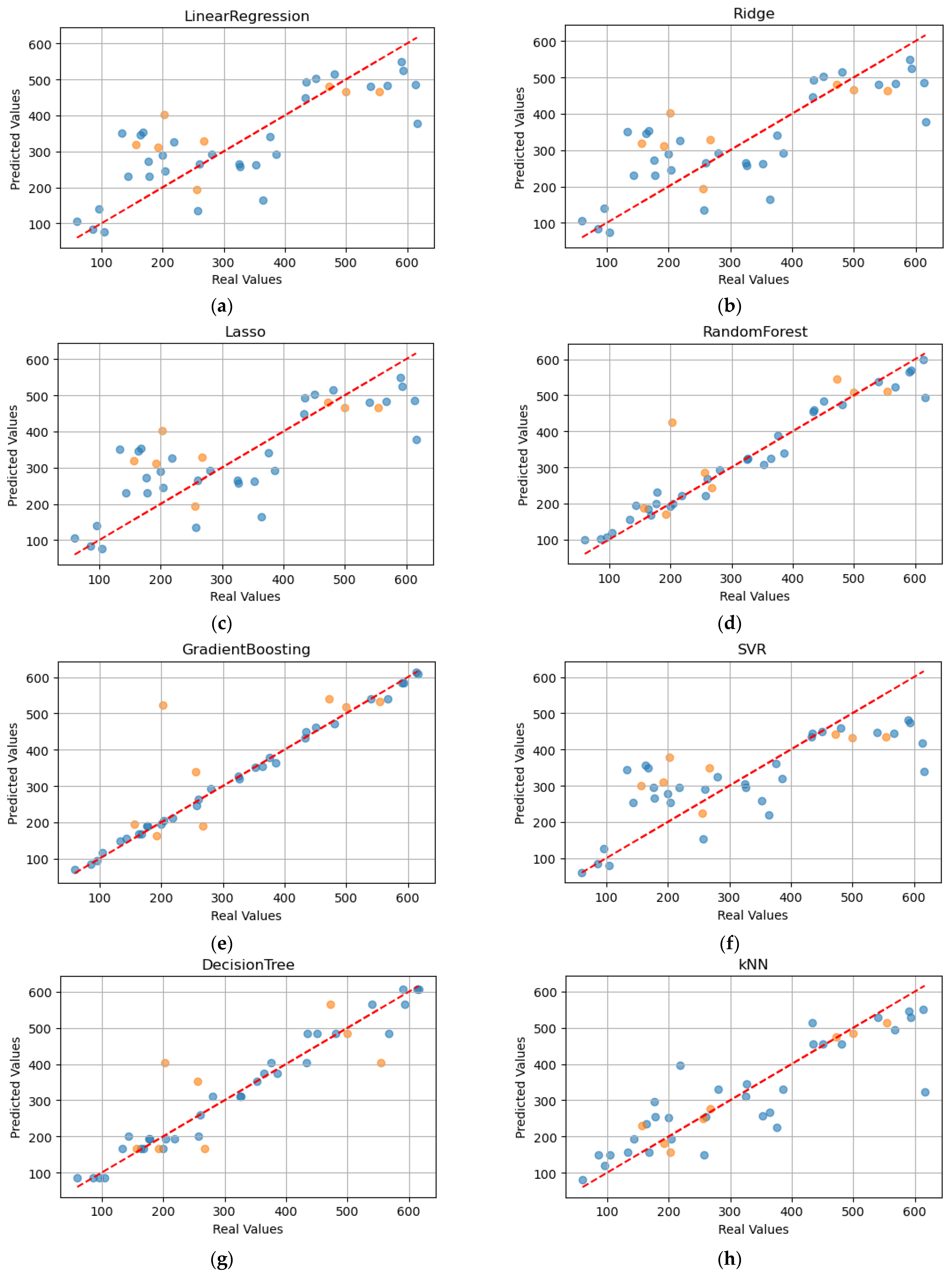
The following scatter plots compare the actual values (“Real Values”) with the predicted values (“Predicted Values”) for the fresh biomass in sweet basil (Figure 6), using different regression models. In general, the dots should be placed along the diagonal (dotted red line), indicating accurate predictions. The blue dots refer to the training prediction values, while the orange dots refer to the testing prediction values.

4. Discussion

The results showed that satellite imagery performed comparably to drone imagery despite the generally lower spatial resolution. Several factors may explain this outcome. First, the spatial resolution of the satellite data used in this study was sufficient to capture field-level variability in a homogeneous crop such as sweet basil, especially given the open-field configuration and uniform canopy coverage. Second, drone imagery may introduce more noise due to flight inconsistencies, illumination variability, or atmospheric interference at low altitudes.

Feature selection results in three different top-ten features. The interesting thing is that only the RFE technique evaluated the predictive variables derived from satellite as important. In contrast, the other two methods focused on variables derived from drones. As a result, eight predictive variables were identified and selected, of which only two refer to vegetation indices calculated by satellite. Drone images, characterized by a higher spatial resolution, allow to calculate more reliable vegetation indices that better explain the characteristics of the crop. The PCA carried out on the eight selected variables reveals that there are three main components which explain almost all the variance.

As regards the performance of regression models, in the training phase, the best results were obtained with RF, GB and DT which achieved an R² of 0.96, 0.99 and 0.97, respectively. In fact, good performance is also attributable to kNN, with an R² of 0.74. However, the test phase involves the use of data that the model has never seen before and, as a result, the real capabilities of the model to predict fresh biomass are tested. In this case, kNN performed better than the others, with an R² of 0.94. An interesting result was also obtained by RF, with an R² of 0.65.

These findings suggest that model complexity does not always guarantee better generalization, and simpler models like kNN may offer better trade-offs between accuracy and robustness, especially when dealing with limited or noisy datasets. Although the test phase simulated prediction on unseen samples, the variability across dates and across environmental- and field-condition practices was limited. Therefore, the authors cannot state that the models are generalizable to other temporal or spatial contexts. Further work is needed to validate the model’s performance on independent datasets collected under different conditions to assess its true predictive robustness and general applicability.

As already mentioned, research on basil in the field is rather limited, and there are no data available in the literature. For this reason, it might be interesting to delve into the regression techniques applicable to fresh biomass prediction. It may also be useful to explore deep learning techniques for more complex problems.

5. Conclusions

Emerging technologies, including drones and artificial intelligence, are profoundly transforming precision agriculture by offering innovative tools for crop monitoring and the optimization of agronomic practices. In this study, we demonstrated how the integration of multi-spectral images acquired from drones and satellites with machine learning algorithms can provide detailed information on the health and productivity of basil in an open field, enabling targeted and timely action.

The results show that advanced image analysis can identify spatial variations in crop conditions with high precision. The use of predictive models based on machine learning techniques has made it possible to correlate vegetation indices with key agronomic parameters, such as productive yield. In particular, the two models which have proven to be the most efficient are Random Forest and k-Nearest Neighbour. These models could be practically applied by farmers and agronomists through user-friendly decision support systems that integrate aerial imagery and provide real-time recommendations on irrigation, fertilization, or harvesting timing, based on predicted crop performance.

The large-scale implementation of these technologies, however, requires further studies to refine the feature selection process and model calibration. The analysis was conducted on a single location and over one crop cycle, which may restrict the generalizability of the results. Furthermore, the small dataset increased the risk of overfitting and poor model stability. As for the bias in model validation, the authors mitigated the effect by applying leave-one-out cross-validation. Future work should focus on expanding the dataset across multiple sites, seasons, and herbs, and on developing a standardized protocol for ad hoc data collection to improve model training and reproducibility. It could be very useful for farmers to manage a time series of aerial imagery during the production season. This choice would allow us to constantly monitor crop status and adjust the agronomic practice.

In conclusion, the integration of multispectral imagery and artificial intelligence into agriculture represents a strategic opportunity to increase crop sustainability and productivity. The evolution of these technologies and their diffusion among farmers will contribute significantly to the transition towards increasingly intelligent, resilient and precision-managed agriculture.

References

- Branca, F.; Treccarichi, S.; Ruberto, G.; Renda, A.; Argento, S. Comprehensive Morphometric and Biochemical Characterization of Seven Basil (Ocimum basilicum L.) Genotypes: Focus on Light Use Efficiency. Agronomy 2024, 14, 224. [Google Scholar] [CrossRef]
- Spence, C. Sweet Basil: An Increasingly Popular Culinary Herb. Int. J. Gastron. Food Sci. 2024, 36, 100927. [Google Scholar] [CrossRef]
- Haas, R.A.; Crișan, I.; Vârban, D.; Vârban, R. Aerobiology of the Family Lamiaceae: Novel Perspectives with Special Reference to Volatiles Emission. Plants 2024, 13, 1687. [Google Scholar] [CrossRef]
- Shahrajabian, M.H.; Sun, W.; Cheng, Q. Chemical Components and Pharmacological Benefits of Basil (Ocimum basilicum): A Review. Int. J. Food Prop. 2020, 23, 1961–1970. [Google Scholar] [CrossRef]
- Yaldiz, G.; Camlica, M. Agro-morphological and Phenotypic Variability of Sweet Basil Genotypes for Breeding Purposes. Crop Sci. 2021, 61, 621–642. [Google Scholar] [CrossRef]
- Mulugeta, S.M.; Gosztola, B.; Radácsi, P. Diversity in Morphology and Bioactive Compounds among Selected Ocimum Species. Biochem. Syst. Ecol. 2024, 114, 104826. [Google Scholar] [CrossRef]
- Schauer, T.; Caspari, C. Guida all’Identificazione Delle Piante; Guide; Zanichelli Editore: Bologna, Italy, 1987; ISBN 978-88-08-03780-0. [Google Scholar]
- ISTAT, Istituto Nazionale di Statistica. Available online: http://dati.istat.it/Index.aspx?QueryId=33707 (accessed on 4 November 2024).
- De Masi, L.; Siviero, P.; Esposito, C.; Castaldo, D.; Siano, F.; Laratta, B. Assessment of Agronomic, Chemical and Genetic Variability in Common Basil (Ocimum basilicum L.). Eur. Food Res. Technol. 2006, 223, 273–281. [Google Scholar] [CrossRef]
- Centorame, L.; Gasperini, T.; Ilari, A.; Del Gatto, A.; Foppa Pedretti, E. An Overview of Machine Learning Applications on Plant Phenotyping, with a Focus on Sunflower. Agronomy 2024, 14, 719. [Google Scholar] [CrossRef]
- Tran, T.; Keller, R.; Trinh, V.; Tran, K.; Kaldenhoff, R. Multi-Channel Spectral Sensors as Plant Reflectance Measuring Devices—Toward the Usability of Spectral Sensors for Phenotyping of Sweet Basil (Ocimum basilicum). Agronomy 2022, 12, 1174. [Google Scholar] [CrossRef]
- Mishra, A.; Matouš, K.; Mishra, K.B.; Nedbal, L. Towards Discrimination of Plant Species by Machine Vision: Advanced Statistical Analysis of Chlorophyll Fluorescence Transients. J. Fluoresc. 2009, 19, 905–913. [Google Scholar] [CrossRef]
- Singla, D.; Gupta, D.; Goyal, N. IoT Based Monitoring for the Growth of Basil Using Machine Learning. In Proceedings of the 2022 10th International Conference on Reliability, Infocom Technologies and Optimization (Trends and Future Directions) (ICRITO), Noida, India, 13–14 October 2022; pp. 1–5. [Google Scholar]
- Son, D.; Park, J.; Lee, S.; Kim, J.J.; Chung, S. Integrating Non-Invasive VIS-NIR and Bioimpedance Spectroscopies for Stress Classification of Sweet Basil (Ocimum basilicum L.) with Machine Learning. Biosens. Bioelectron. 2024, 263, 116579. [Google Scholar] [CrossRef] [PubMed]
- Jeon, Y.-J.; Kim, H.S.; Lee, T.S.; Park, S.H.; Choi, H.-B.; Jung, D.-H. Efficient Detection of Drought Stress Responses in Basil (Ocimum basilicum L.) Via 3d-Cnn-Based Phenotyping Data Fusion Approach. 2024. Available online: https://www.ssrn.com/abstract=4801293 (accessed on 12 February 2025).
- Tucker, C.J.; Elgin, J.H.; McMurtrey, J.E.; Fan, C.J. Monitoring Corn and Soybean Crop Development with Hand-Held Radiometer Spectral Data. Remote Sens. Environ. 1979, 8, 237–248. [Google Scholar] [CrossRef]
- Gitelson, A.A.; Kaufman, Y.J.; Merzlyak, M.N. Use of a Green Channel in Remote Sensing of Global Vegetation from EOS-MODIS. Remote Sens. Environ. 1996, 58, 289–298. [Google Scholar] [CrossRef]
- Barnes, E.; Clarke, T.R.; Richards, S.E.; Colaizzi, P.; Haberland, J.; Kostrzewski, M.; Waller, P.; Choi, C.; Riley, E.; Thompson, T.L. Coincident Detection of Crop Water Stress, Nitrogen Status, and Canopy Density Using Ground Based Multispectral Data. In Proceedings of the Fifth International Conference on Precision Agriculture, Bloomington, MN, USA, 16–19 July 2000. [Google Scholar]
- Datt, B.; McVicar, T.R.; Van Niel, T.G.; Jupp, D.L.B.; Pearlman, J.S. Preprocessing Eo-1 Hyperion Hyperspectral Data to Support the Application of Agricultural Indexes. IEEE Trans. Geosci. Remote Sens. 2003, 41, 1246–1259. [Google Scholar] [CrossRef]
- Huete, A.; Didan, K.; Miura, T.; Rodriguez, E.P.; Gao, X.; Ferreira, L.G. Overview of the Radiometric and Biophysical Performance of the MODIS Vegetation Indices. Remote Sens. Environ. 2002, 83, 195–213. [Google Scholar] [CrossRef]
- Huete, A.R. A Soil-Adjusted Vegetation Index (SAVI). Remote Sens. Environ. 1988, 25, 295–309. [Google Scholar] [CrossRef]
- Tao, P.; Yi, H.; Wei, C.; Ge, L.Y.; Xu, L. A Method Based on Weighted F-Score and SVM for Feature Selection. In Proceedings of the 2013 25th Chinese Control and Decision Conference (CCDC), Guiyang, China, 25–27 May 2013; pp. 4287–4290. [Google Scholar]
- Polat, K.; Güneş, S. A New Feature Selection Method on Classification of Medical Datasets: Kernel F-Score Feature Selection. Expert Syst. Appl. 2009, 36, 10367–10373. [Google Scholar] [CrossRef]
- Ilango, B.S.; Ramaraj, N. A Hybrid Prediction Model with F-Score Feature Selection for Type II Diabetes Databases. In Proceedings of the 1st Amrita ACM-W Celebration on Women in Computing in India, Coimbatore India, 16–17 September 2010; pp. 1–4. [Google Scholar]
- Song, Q.; Jiang, H.; Liu, J. Feature Selection Based on FDA and F-Score for Multi-Class Classification. Expert Syst. Appl. 2017, 81, 22–27. [Google Scholar] [CrossRef]
- Sevani, N.; Hermawan, I.; Jatmiko, W. Feature Selection Based on F-Score for Enhancing CTG Data Classification. In Proceedings of the 2019 IEEE International Conference on Cybernetics and Computational Intelligence (CyberneticsCom), Banda Aceh, Indonesia, 22–24 August 2019; pp. 18–22. [Google Scholar]
- Yan, K.; Zhang, D. Feature Selection and Analysis on Correlated Gas Sensor Data with Recursive Feature Elimination. Sens. Actuators B Chem. 2015, 212, 353–363. [Google Scholar] [CrossRef]
- Misra, P.; Yadav, A.S. Improving the Classification Accuracy Using Recursive Feature Elimination with Cross-Validation. Int. J. Emerg. Technol. 2020, 11, 659–665. [Google Scholar]
- Hamada, M.; Tanimu, J.J.; Hassan, M.; Kakudi, H.A.; Robert, P. Evaluation of Recursive Feature Elimination and LASSO Regularization-Based Optimized Feature Selection Approaches for Cervical Cancer Prediction. In Proceedings of the 2021 IEEE 14th International Symposium on Embedded Multicore/Many-core Systems-on-Chip (MCSoC), Singapore, 20–23 December 2021; pp. 333–339. [Google Scholar]
- Uddin, M.T.; Uddiny, M.A. A Guided Random Forest Based Feature Selection Approach for Activity Recognition. In Proceedings of the 2015 International Conference on Electrical Engineering and Information Communication Technology (ICEEICT), Savar, Dhaka, Bangladesh, 21–23 May 2015; pp. 1–6. [Google Scholar]
- Hasan, M.A.M.; Nasser, M.; Ahmad, S.; Molla, K.I. Feature Selection for Intrusion Detection Using Random Forest. J. Inf. Secur. 2016, 7, 129–140. [Google Scholar] [CrossRef]
- Iranzad, R.; Liu, X. A Review of Random Forest-Based Feature Selection Methods for Data Science Education and Applications. Int. J. Data Sci. Anal. 2024. [Google Scholar] [CrossRef]
- Mishra, S.; Mishra, D.; Das, S.; Rath, A.K. Feature Reduction Using Principal Component Analysis for Agricultural Data Set. In Proceedings of the 2011 3rd International Conference on Electronics Computer Technology, Kanyakumari, India, 8–10 April 2011; pp. 209–213. [Google Scholar]
- Karamizadeh, S.; Abdullah, S.M.; Manaf, A.A.; Zamani, M.; Hooman, A. An Overview of Principal Component Analysis. J. Signal Inf. Process. 2013, 4, 173–175. [Google Scholar] [CrossRef]
- Daffertshofer, A.; Lamoth, C.J.C.; Meijer, O.G.; Beek, P.J. PCA in Studying Coordination and Variability: A Tutorial. Clin. Biomech. 2004, 19, 415–428. [Google Scholar] [CrossRef]
- Abdi, H.; Williams, L.J. Principal Component Analysis. WIREs Comput. Stats 2010, 2, 433–459. [Google Scholar] [CrossRef]
- Meng, J.; Yang, Y. Symmetrical Two-Dimensional PCA with Image Measures in Face Recognition. Int. J. Adv. Robot. Syst. 2012, 9, 238. [Google Scholar] [CrossRef]
- Hope, T.M.H. Linear Regression. In Machine Learning; Elsevier: Amsterdam, The Netherlands, 2020; pp. 67–81. ISBN 978-0-12-815739-8. [Google Scholar]
- Montgomery, D.C.; Peck, E.A.; Vining, G.G. Introduction to Linear Regression Analysis, 6th ed.; Wiley Series in Probability and Statistics; Wiley: Hoboken, NJ, USA, 2021; ISBN 978-1-119-57872-7. [Google Scholar]
- Rajan, M.P. An Efficient Ridge Regression Algorithm with Parameter Estimation for Data Analysis in Machine Learning. SN Comput. Sci. 2022, 3, 171. [Google Scholar] [CrossRef]
- Nakatsu, R.T. Validation of Machine Learning Ridge Regression Models Using Monte Carlo, Bootstrap, and Variations in Cross-Validation. J. Intell. Syst. 2023, 32, 20220224. [Google Scholar] [CrossRef]
- Tibshirani, R. Regression Shrinkage and Selection Via the Lasso. J. R. Stat. Soc. Ser. B Stat. Methodol. 1996, 58, 267–288. [Google Scholar] [CrossRef]
- Roth, V. The Generalized LASSO. IEEE Trans. Neural Netw. 2004, 15, 16–28. [Google Scholar] [CrossRef]
- Ranstam, J.; Cook, J.A. Statistical Models: An Overview. Br. J. Surg. 2016, 103, 1047. [Google Scholar] [CrossRef] [PubMed]
- Zhang, F.; O’Donnell, L.J. Support Vector Regression. In Machine Learning; Elsevier: Amsterdam, The Netherlands, 2020; pp. 123–140. ISBN 978-0-12-815739-8. [Google Scholar]
- Üstün, B.; Melssen, W.J.; Buydens, L.M.C. Visualisation and Interpretation of Support Vector Regression Models. Anal. Chim. Acta 2007, 595, 299–309. [Google Scholar] [CrossRef] [PubMed]
- Myles, A.J.; Feudale, R.N.; Liu, Y.; Woody, N.A.; Brown, S.D. An Introduction to Decision Tree Modeling. J. Chemom. 2004, 18, 275–285. [Google Scholar] [CrossRef]
- Navada, A.; Ansari, A.N.; Patil, S.; Sonkamble, B.A. Overview of Use of Decision Tree Algorithms in Machine Learning. In Proceedings of the 2011 IEEE Control and System Graduate Research Colloquium, Shah Alam, Malaysia, 27–28 June 2011; pp. 37–42. [Google Scholar]
- De Ville, B. Decision Trees. WIREs Comput. Stats 2013, 5, 448–455. [Google Scholar] [CrossRef]
- Somvanshi, M.; Chavan, P.; Tambade, S.; Shinde, S.V. A Review of Machine Learning Techniques Using Decision Tree and Support Vector Machine. In Proceedings of the 2016 International Conference on Computing Communication Control and automation (ICCUBEA), Pune, India, 12–13 August 2016; pp. 1–7. [Google Scholar]
- Breiman, L. Random Forests. Mach. Learn. 2001, 45, 5–32. [Google Scholar] [CrossRef]
- Svetnik, V.; Liaw, A.; Tong, C.; Culberson, J.C.; Sheridan, R.P.; Feuston, B.P. Random Forest: A Classification and Regression Tool for Compound Classification and QSAR Modeling. J. Chem. Inf. Comput. Sci. 2003, 43, 1947–1958. [Google Scholar] [CrossRef]
- Rodriguez-Galiano, V.; Sanchez-Castillo, M.; Chica-Olmo, M.; Chica-Rivas, M. Machine Learning Predictive Models for Mineral Prospectivity: An Evaluation of Neural Networks, Random Forest, Regression Trees and Support Vector Machines. Ore Geol. Rev. 2015, 71, 804–818. [Google Scholar] [CrossRef]
- Natekin, A.; Knoll, A. Gradient Boosting Machines, a Tutorial. Front. Neurorobot. 2013, 7, 21. [Google Scholar] [CrossRef]
- Konstantinov, A.V.; Utkin, L.V. Interpretable Machine Learning with an Ensemble of Gradient Boosting Machines. Knowl. Based Syst. 2021, 222, 106993. [Google Scholar] [CrossRef]
- Cunningham, P.; Delany, S.J. K-Nearest Neighbour Classifiers—A Tutorial. ACM Comput. Surv. 2022, 54, 128. [Google Scholar] [CrossRef]
- Song, Y.; Liang, J.; Lu, J.; Zhao, X. An Efficient Instance Selection Algorithm for k Nearest Neighbor Regression. Neurocomputing 2017, 251, 26–34. [Google Scholar] [CrossRef]
- Zhang, S.; Li, X.; Zong, M.; Zhu, X.; Cheng, D. Learning k for kNN Classification. ACM Trans. Intell. Syst. Technol. 2017, 8, 43. [Google Scholar] [CrossRef]
- Zhang, S. Challenges in KNN Classification. IEEE Trans. Knowl. Data Eng. 2022, 34, 4663–4675. [Google Scholar] [CrossRef]
- Tatachar, A.V. Comparative Assessment of Regression Models Based On Model Evaluation Metrics. Int. Res. J. Eng. Technol. 2021, 8, 2395-0056. [Google Scholar]
- Chicco, D.; Warrens, M.J.; Jurman, G. The Coefficient of Determination R-Squared Is More Informative than SMAPE, MAE, MAPE, MSE and RMSE in Regression Analysis Evaluation. PeerJ Comput. Sci. 2021, 7, e623. [Google Scholar] [CrossRef]
Figure 1.
RGB orthomosaic obtained using a drone, elaborated with QGis.
Figure 2.
Workflow of the proposed methodology from the acquisition of field data (both parameters measured on the ground and remotely) to the analysis of data using machine learning techniques (blue dots represents training predictions, while orange dots represents testing predictions). The aim is to provide a support tool for farmers.
Figure 3.
The tools used for data collection are as follows: (a) wheel metre for height measurement; (b) cardboard frame to delimit the sample area.
Figure 4.
Route flight on DJI Pilot application.
Figure 5.
Principal Component Analysis of the most important feature selected through F1-score-, RFE- and RF-based selection. The blue bars represent the variance explained by each component, while the dashed red line highlights the cumulative explained variance.
Figure 6.
Scatter plots are useful for graphically representing the accuracy of trained models to predict basil fresh biomass. In detail, the x-axis shows the real values, contrasting the y-axis, which shows the predicted values. The blue dots refer to the training prediction; meanwhile, the orange dots refer to the testing prediction. Each model is represented: (a) Linear Regression; (b) Ridge Regression; (c) LASSO regression; (d) Random Forest; (e) Gradient Boosting; (f) Support Vector Regression; (g) Decision Tree; (h) k-Nearest Neighbours.