Abstract
This study presents a novel approach to passive human counting in indoor environments using Bluetooth Low Energy (BLE) signals and deep learning. The motivation behind this research is the need for non-intrusive, privacy-preserving occupancy monitoring in sensitive indoor settings, where traditional camera-based solutions may be unsuitable. Our method leverages the deformations that BLE signals undergo when interacting with the human body, enabling occupant detection and counting without requiring wearable devices or visual tracking. We evaluated three deep neural network models—Convolutional Neural Network (CNN), Long Short-Term Memory (LSTM), and a hybrid CNN+LSTM architecture—under both classification and regression settings. Experimental results indicate that the hybrid CNN+LSTM model outperforms the others in terms of accuracy and mean absolute error. Notably, in the regression setup, the model can generalize to occupancy values not present in the fine-tuning dataset, requiring only a few minutes of calibration data to adapt to a new environment. We believe that this approach offers a valuable solution for real-time people counting in critical environments such as laboratories, clinics, or hospitals, where preserving privacy may limit the use of camera-based systems. Overall, our method demonstrates high adaptability and robustness, making it suitable for practical deployment in diverse indoor scenarios.
1. Introduction
The ability to estimate the number of occupants in an interior space has a variety of practical applications, including the optimization of heating, ventilation and air conditioning (HVAC) or lighting for energy saving, comfort improvement, building automation, and surveillance [1]. It can also be particularly important for the protection of people in the event of natural or man-made disasters and other emergency scenarios [2]. Furthermore, in privacy-sensitive environments such as hospitals, clinics, or laboratories, real-time people counting can support both safety and operational efficiency, provided that the monitoring solutions adopted do not rely on intrusive technologies such as cameras, which may raise privacy concerns and even cause discomfort among workers [3].
Various technologies have been used to detect and count people in indoor settings, ranging from infrared barriers to computer vision to radio frequency (RF) and radar-like sensing [4]. These can be classified according to the requirement that the sensed human carries a device (device-based versus device-less sensing) and the ability of the sensing device to both emit and receive the signal used to detect the human (active versus passive sensing) [5]. The choice of approach and technologies adopted to detect, count, or locate human beings in bounded areas and possibly track their movements and activities depends on the specific context and design constraints [6]. For example, tracking an employee by exploiting some miniaturized device attached to their badge is acceptable, as long as adequate information is provided to them for privacy reasons. In contrast, device-based sensing of visitors in public buildings might not be the most convenient approach, unless visitors need to wear a badge for some other reason. Consequently, if the wearing or carrying of a device is not desirable, device-less sensing is preferable [7]. Several methods have also been explored to monitor people in crowded environments by exploiting the signals emitted by smartphones and other handheld/portable devices that people carry with them consistently [8].
In the last decade, the rapid development of machine learning technology and the introduction of stringent privacy protection regulations (e.g., GDPR in the European Union) have generated a great deal of interest in passive human sensing based on RF, referring to different methods adopted to analyze the deformation that an RF signal undergoes when traversing a human body (see Figure 1), and to extract information regarding the presence and activity of humans in the area covered by the analyzed signal [7]. Ultra-wideband radar technology (UWB) has been demonstrated to be very powerful and effective in passively detecting and monitoring people and their vital signs [9,10,11] but requires ad hoc devices to be produced and deployed in the monitored environment, which increases the costs and may raise some coexistence issues with the wireless communication infrastructures already installed in the same area. While coexistence issues can be mitigated by exploiting adequate techniques [12], the costs of producing and deploying ad hoc hardware for passive sensing still require a cheap and widely available solution.
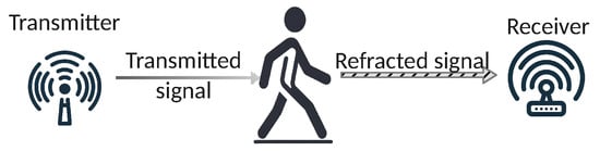
Figure 1.
Passive human sensing through the analysis of RF signals traversing a human body.
As a consequence, the application of commercial off-the-shelf (COTS) WiFi technology to passive human sensing has been widely exploited [13,14,15], while fewer works have addressed the combination of communication-oriented and radar-oriented technologies [16].
WiFi has the specific ability to provide Channel State Information (CSI), a comprehensive and punctual description of the state of the receiving channel that allows an accurate analysis of the deformation of the received signal, also with respect to its phase and frequency [17]. Furthermore, the high speed of WiFi allows for a high sampling rate, which makes it possible to estimate vital signs [18] and motion parameters [19] of the individuals being monitored.
The application of Bluetooth Low Energy (BLE) to passive sensing has also been investigated as a convenient alternative to WiFi for several reasons, ranging from its lower power consumption to lower costs, easier deployment, and lower impact on existing wireless communication infrastructure [6,20]. However, the BLE protocol still retains some features that make it less flexible for passive human sensing, compared to WiFi:
- The passive human sensing application cannot extract from the received message the BLE frequency information, which would be needed to better cope with the variation in RSSI according to the transmission channel. Specifically, the application layer does not provide access to the frequency (that is, the channel) chosen by the Adaptive Frequency Hopping (AFH) mechanism of the BLE protocol to send a message. This constraint is related to security and is not expected to be relaxed in the near future.
- WiFi Channel State Information (CSI) can be directly acquired from certain devices using the WiFi multicarrier encoding mechanism, whereas BLE does not support this type of measurement.
- Acquiring RSSI samples at high rates from BLE-based devices is a challenge. Consequently, collecting the substantial amount of data necessary to train a machine learning model requires a sensibly long "idle" period before the model can be deployed, which may not be feasible for many practical applications [21].
Due to the above issues, the literature reports mainly on applications of BLE to simple passive human detection [20,22,23] and only a few research works deal with approximate people counting [24,25]. Conversely, in this paper, we present an approach to passive people counting in indoor environments, based on BLE and a deep learning model, which to our knowledge is the first in the literature that features an accuracy similar to those based on WiFi, while only requiring a quick fine-tuning session to adapt to a new environment and relying both on LoS and non-LoS (reflected) propagation.
The main contributions of this work are the following.
- We tested and compared five different deep learning architectures on a large dataset, in order to select the one that performs best.
- Model fine-tuning. Instead of retraining the model from scratch for each deployment, we collected a large and heterogeneous dataset and used it to pre-train and validate the model. For each new deployment, we then acquire a small dataset from the unknown environment and use it to fine-tune the model. The procedure is quick and accurate, since only about 4000 samples are used.
- High accuracy. The proposed approach can obtain a people count accuracy higher than 99% (according to the accuracy metrics used in the literature) or 96% (according to the more strict metric we adopted) with only a few minutes of training data acquisition in a completely unknown indoor environment, provided that a sufficient number of people can be asked to enter and exit the room during a few minutes interval. The appropriate number of people to involve is equal to, or greater than, the largest number of occupants expected to be counted by the model in the specific environment where it is being fine-tuned.
- High resolution of the people count. If we define the resolution of the people count as the minimum difference between two measurements that can be discriminated by the proposed system, we can consider as optimal a resolution equal to 1. The proposed approach has been evaluated and validated by setting the resolution to 1, that is, to the optimal resolution.
- Interpolation ability. At the cost of a reasonable accuracy degradation, the proposed approach can be easily fine-tuned based only on a suboptimal number of cases, that is, for example, by acquiring samples only with 1-5-9 persons in a room and still being able to count from 0 to 10 occupants. In other words, it can estimate a never-seen-before number of occupants, provided that such a number is not too far from those that it has seen. To the best of our knowledge, this result has never been presented in the literature before.
This paper is organized as follows.
Section 2 introduces the relevant literature on passive human sensing based on BLE. In Section 3, an overview of the proposed approach to BLE-based passive human sensing is presented. Section 3.1 describes the data gathering and pre-processing procedure, whereas Section 3.2 describes the proposed deep neural model. Section 4 illustrates the setup and deployments adopted for our experiments, and Section 5 reports on the experimental results obtained. Finally, Section 6 presents our conclusions.
2. Related Work
In recent years, activities such as passive human detection [20,23], counting [24,26], and motion tracking [27] using BLE have been investigated in the literature, although in most cases the described approaches obtained lower accuracy than their WiFi counterparts [6,28].
In [24], a BLE-based human sensing architecture is proposed that is capable of counting the occupants of a lecture room. With 24 beacons placed under the seats in the room and four receivers positioned on the ceiling laterally to the seats, the detection accuracy was higher than 95%, while the root mean square error (RMSE) of the predicted number of occupants was ≈5.42. Providing only the RMSE of the count measure is not sufficient to assess the performance of the proposed approach, as the average number of occupants is not reported, and therefore, it is not possible to evaluate the fraction (that is, percentage) of miscounted occupants with respect to the real number of occupants. Furthermore, the proposed method relies mainly on the attenuation of the BLE RSSI Line of Sight (LoS) signal on the receiving side due to direct occlusion by the people’s bodies, so it is not clear how it would perform if a different deployment of transmitters and receivers is enforced by environmental constraints. Finally, the proposed method requires the manual measurement of the distances between each transmitter and each receiver.
In [26], a classroom environment is examined where a Radial Basis Function Neural Network is employed to classify RSSI samples. These samples are generated by strategically placed BLE beacons and received by a BLE receiver, with the number of occupants in the room varying. However, the dataset used in the experiments is not publicly accessible, and the paper lacks sufficient detail to allow for replication of the study.
In [22], a reinforcement learning approach is introduced for passive human detection using BLE RSSI data (without performing occupancy counting). The system leverages feedback from sensors and other IoT devices to guide the learning process. While the method is described as adaptive to environmental changes, it requires an initial fine-tuning phase. Moreover, its performance is comparable to that of simpler statistical methods, such as the one presented in [20].
In [25], a BLE-based passive human counting system is evaluated against state-of-the-art WiFi-based alternatives. The proposed architecture, however, necessitates manual measurement of distances between transmitters and receivers during the training phase. Additionally, optimal performance is achieved only when the sensing network operates at very high sampling rates (up to 200 Hz), which significantly exceeds the standard advertisement rate of typical BLE beacons. Moreover, the experimental results presented only take into account up to five persons in a room, and in most cases, only up to two. As a consequence, it is not clear how the model scales with the number of occupants.
The approach proposed in this paper does not rely on the measurement of the transmitter–receiver distances nor on specific LoS signal occlusion. Moreover, it does not require a full model retraining for each unknown environment, but only a short fine-tuning and, furthermore, has been tested with a number of occupants that varied with a step of 1 from 0 to 10, thus allowing a precise estimation of its performance.
3. BLE-Based Passive Human Sensing
Radio Frequency (RF)-based passive human sensing (PHS) takes advantage of the modification induced in the RF signal by the presence of a human body along its pathway. When traversing a human body, the radio signal is refracted and attenuated, thus undergoing changes in its phase and intensity (see Figure 2). The signal can also be refracted and reflected by objects, furniture, and walls, thus generating multipath signals. All these types of signals must be captured, filtered, and analyzed for PHS [23]. A general investigation of the effects of reflected and refracted components of the received signal on the accuracy and reliability of the passive detection process was investigated in several seminal works, such as in [29] and is outside the scope of this paper.
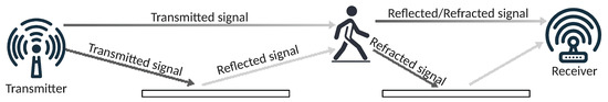
Figure 2.
Line of Sight (LoS) and Multipath (Non-LoS) PHS. Note that multiple signals traverse the same obtruding human body from different angles and with different time (phase) shifts, thus transporting spatially and temporally diverse information.
Unlike the changes induced by the presence of fixed obstacles and signal reflections, which may combine into constructive or destructive interference but in general do not show significant time dynamics, the deformations induced by human bodies change in time according to people’s movements and physiological fluctuations, for example, due to respiration and heartbeat. The time dynamics of human-induced deformation of RF signals has been widely investigated, for example, for the detection and analysis of vital signs based on WiFi [18].
The BLE protocol does not support the kind of direct measurement of highly detailed channel information (e.g., CSI) exploited by WiFi-based PHS approaches [6]. However, the Received Signal Strength Information (RSSI) variations contain sufficient information to allow human detection and counting, provided that the RSSI is adequately filtered to remove noise and unwanted variations, and that a reliable predictive model is adopted. In fact, due to frequent changes in pose, location, and physiological dynamics (for example, respiration), the RSSI deformation caused by the presence of a human body is affected by high variability, as shown in Figure 3.
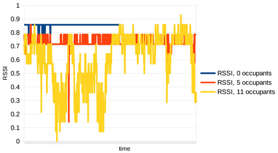
Figure 3.
Graph of the variations in RSSI in time, for the cases: 0-person occupancy, 5-person occupancy, 11-person occupancy. Note that people in the room moved often and the variability due to people motion increases with the number of persons in the room.
Furthermore, due to security constraints, the Adaptive Frequency Hopping (AFH) mechanism in BLE prevents the sensing applications from retrieving from the BLE interface the specific channel on which a message was received. Since the RSSI exhibits distinct mean values across different channels [30], frequency hopping introduces significant variability in the RSSI distribution. This variability negatively impacts the classification accuracy of most BLE-based passive human sensing (PHS) methods. To address this issue, the approach adopted in this paper follows the strategy proposed in [27], wherein the transmitter is configured to operate on a fixed channel.
We propose a sensing architecture composed of BLE beacons (the transmitters) and BLE receivers. BLE beacons are low-cost, low-power devices that only broadcast advertising frames, marked with a unique device identifier. In our case, the beacons are set to transmit on a fixed channel that is specified at the configuration time. Receivers are also low-cost, low-power, BLE-enabled devices that receive the advertising frames, add a receiver identifier and a timestamp, and send them as a data stream to a server that analyzes all the received data and produces an occupancy estimate for each area of interest in near-real time. This architecture potentially also allows for passive person localization, but this application is not covered in this paper.
The number of transmitters and receivers is only constrained by the condition that each occupant of the monitored area is traversed (either in LoS or after a reflection) by the signal emitted by at least one of the transmitters and received by at least one of the receivers. All transmitters and receivers are supposed to be fixed in space, that is, they should not be moved after their initial deployment. If one or more devices are moved, a reiteration of the calibration (fine-tuning) phase is required (see Section 3.2).
3.1. Data Gathering and Pre-Processing
At each receiving node, sample queues are managed (see Figure 4). Each sample refers to an advertisement frame transmitted by a beacon and received by the receiving node and contains a reception timestamp, the identifier of the transmitter (the beacon), the identifier of the receiving node, and the RSSI value measured upon reception.
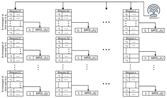
Figure 4.
Diagram of the data processing workflow at a generic receiver r. For each transmitter, the incoming samples are grouped into sets of k. From each group, a representative sample is selected as the ”median”of the k values, and it retains its original timestamp. The notation indicates that the samples within each group are collected at times approximately equal to , meaning they share closely aligned timestamps.
Since the transmitter and receiver are not time-synchronized, it is not feasible to leverage the phase shift of multiple messages with identical timestamps to enhance spatial resolution [31]. As a result, this work prioritizes robustness to noise over temporal resolution (i.e., the PHS sampling frequency). To achieve this, we aggregate the RSSI values from k messages, each transmitted by the same beacon i and received by receiver r, that share closely aligned timestamps around time t.
This aggregation is performed by calculating the median of the k RSSI values, which we refer to as the Median RSSI Sample received by the receiver r at time t ().
This procedure significantly mitigates the impact of abrupt, undesired fluctuations in RSSI, such as those caused by human movement, but it also reduces the temporal resolution by a factor of k.
At each receiver, and for every time instant j at which a message is received, the median RSSI values from different beacons that share similar timestamps are compiled into a single row, labeled with the representative timestamp j. As a result, each receiver r maintains a list, denoted as , where each row corresponds to a specific time instant j and contains a sequence of values that are the median RSSI values received from the various beacons around that time.
These lists () are then transmitted to a central Processing Node (PN), which merges them into a unified list and sorts the entries by their representative timestamps. This consolidated list is used as input for estimating the number of occupants. At this stage, the temporal resolution is sufficiently coarse that any lack of synchronization between the receivers and the central server becomes negligible. Given that BLE 4.x typically transmits advertising messages every 100 ms, the effective sampling rate at this point in the algorithm is samples per second. The PN then feeds the merged list into a deep neural network model, which outputs an estimate of the number of people present in the monitored area.
3.2. The Proposed Deep Learning Model
In the literature, both classification and regression have been used for Passive Human Counting (PHC).
Classification is often the simpler approach, depending on the specific classification technique used [32,33]. Furthermore, measuring classification performance by counting the percentage of correct predictions, i.e., calculating its accuracy, also provides an understandable evaluation of the reliability of the proposed approach, which is valuable information when the main motivation for the work is the safety of people.
Regression is conceptually better suited to a numerical estimation problem, such as the one at hand [24,25]. However, the quantities being predicted are discrete and finite numbers and may as well be considered as non-numeric labels, thus suggesting the use of classification instead. Nevertheless, regression retains the important advantage that it allows for estimating values that the model has never seen before, that is, the regressive model can in principle predict an occupancy value that it has not been trained on. As will be shown in Section 5, this occurs at the cost of performance degradation, but it can still be carried out with regression, while most classification techniques would not support it. Some interesting work in the classification literature can deal with unseen labels, but at the cost of a severe increase in computational complexity and a significant degradation in accuracy [34].
We tested five different deep neural network models, characterized by increasing complexity and based on widely adopted architectures [35]:
- 1.
- A Dense Neural Network model (DenseNN), composed of a stack of three dense layers.
- 2.
- A Convolutionary Neural Network (CNN), composed of three Convolutionary layers.
- 3.
- A Long Short-Term Memory (LSTM) network, composed of two Long Short-term Memory (LSTM) layers.
- 4.
- A hybrid CNN+LSTM network structured as a sequence of three Convolutionary layers followed by two LSTM layers.
- 5.
- A legacy Transformer model with four heads, four Transformer blocks, and .
In all five architectures, the model was completed by an output dense layer in two different settings, i.e., a classification task and a regression task.
In each model, only the last two layers change according to the setting. In the classification models, the final "dense" layer uses a Softmax activation function, whereas in the regression models, the final "dense" layer uses a linear activation function. All CNN layers in the models use a ReLU activation function, and all models are trained with the Adam optimizer. Furthermore, the classification models are trained using the Sparse Categorical Cross-Entropy Loss Function, whereas the regression models are trained using the Mean Squared Error Loss Function.
Each architecture presents unique strengths and limitations, which are summarized below (Table 1).

Table 1.
Comparative analysis of deep learning architectures.
The approach presented is based on pre-training and fine-tuning a deep learning model, thus improving the final accuracy of the prediction. More specifically, the model was pre-trained and validated using a large dataset collected during several hours in different rooms and with different numbers of occupants sitting in different places. When collecting such data, an operator manually annotated the number of occupants. Subsequently, a smaller dataset was gathered during a few minutes session in the same environment (that is, in the same room) where the final test dataset was gathered, thus letting the model learn about the internal geometry of the testing environment. From the point of view of the final user, fine-tuning recalls the calibration of a measurement instrument before deploying it in production.
Fine-tuning is a crucial step for the application at hand. The performance of the model depends on its implicit knowledge of the deployment geometry of the BLE transmitters and receivers involved. Consequently, several works in the literature propose to manually measure the distance between each transmitter and each receiver, in addition to fully training the model on data collected in the same environment and setup as the test data. Here, instead, we pre-train each model on a large, heterogeneous dataset and then fine-tune it on a much smaller dataset, gathered in the same setup and environment as the test dataset. We show in Section 5 that with such a simpler and faster procedure, the model outperforms all other approaches in the literature.
Comparing classification and regression models on the same task is not straightforward. In [25,44], the performance of the regression models is evaluated in terms of the percentage of predictions that fall within where is the true value, i.e., the correct value that the model must predict.
Such a large interval corresponds to a resolution coarser than 1 and is questionable, as shown by the following simple example. If the correct value is, say, 5 and the predicted value is 4, the prediction will still be considered correct according to the chosen interval, but it is indeed not correct because the model is predicting a value that corresponds to a wrong occupancy. Therefore, in our experiments, we consider the narrower interval , which corresponds to the most common approximation of a real-valued number to an integer. As a consequence, to evaluate the performance of a regressive model in terms of accuracy-like metrics, we measure the percentage of predictions that, when approximated to an integer, exactly match the true value. This metric is also known as the Almost-Correct Prediction Rate (ACPR), and we use it, setting , together with the mean absolute error to evaluate the performance of the regressive models.
4. Experimental Setup
The pre-training and validation dataset used for this paper was built by gathering data during several hours in 3 different rooms of about 50 square meters each, with different dispositions of the workstations and different numbers of occupants, ranging from 1 to 11.
In all rooms, 5 transmitters and 2 receivers were deployed. The collected samples were grouped into a single large dataset and then processed according to the procedure described in Section 3.1, thus producing a dataset of approximately 20,000 samples. The actual occupancy information was manually added by an operator who attended each data acquisition session. This dataset was used to pre-train the model, validate it, and preliminarily test it. To this end, the dataset was partitioned into three subsets (namely, the Pre-Training, Pre-Training Validation, and Pre-Training Test datasets).
For the sake of generality of the pre-trained model, any bias and information on the prior probability distribution of the elements in each class (one class per each integer number of occupants in the range ), must be canceled; therefore, we randomized the samples in each dataset (that is, randomly re-sampled the datasets) in order to remove their original ordering information and balanced the number of elements in each class as follows:
- 1.
- Set the target per-class cardinality (PCC) as the median number of elements across the classes.
- 2.
- Subsample all the classes that have a number of elements larger than PCC, so that all classes have at most PCC elements.
- 3.
- Augment the classes that have fewer than PCC elements.
Data augmentation requires that, in those classes that do not contain a sufficient number of samples (weak classes), new samples are generated based on existing ones, by duplicating and slightly transforming them, for example, with additive noise (jitter), randomly distributed translations, and magnitude warping [45]. In our experimental setup, we adopted the data augmentation procedure described in [46] to balance the classes in our datasets. Figure 5a shows an example of an unbalanced dataset used in our experiments, and Figure 5b shows the effects of augmenting the weak classes in the same dataset.
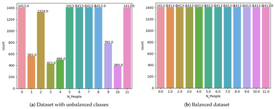
Figure 5.
(a) An unbalanced dataset used in our experiment. (b) The effects of the data augmentation approach adopted in our experimental setup.
After the above procedure, the datasets contain the same number of samples per class, thus reducing the risk of bias. Moreover, the uniform Per-Class Cardinality (PCC) of the datasets, i.e., the fact that all classes in a dataset have the same number of elements, is also maintained in the Pre-Training Test dataset, thus allowing us to use accuracy as a reliable classification performance metrics [47].
A separate dataset for testing the fine-tuning approach was collected from a different room, a 60 square meter laboratory equipped with the same number of transmitters and receivers as in the rooms mentioned above. The occupants entered and left the room during the data acquisition session, and their number (ranging from 0 to 10) was manually annotated with a dedicated application at each change. This dataset contains about 15,000 samples evenly distributed among the 11 classes and was also partitioned into a Fine-Tuning Training, a Fine-Tuning Validation, and a Fine-Tuning Test dataset.
Both the transmitting and receiving devices were developed using the standard BLE application interface available on the low-cost, low-power Banana PI M5 single-board computer, running the Linux Operating System, and equipped with 4GB RAM memory, Amlogic S905X3 64-bit quad-core Cortex A55 processor, Mali G31 GPU, and a BL-M8821CU1 Wifi and BLE 4.2 expansion board. The transmitting devices duly emulated the behavior of commercial BLE 4.2 beacons.
The datasets collected and employed in the experiments are included as Supplementary Material associated with the article.
Training and fine-tuning were carried out on a notebook computer running the Linux operating system and equipped with an Nvidia GTX 1650Ti GPU.
5. Experimental Results
Experiments were conducted to evaluate the performance of the five models (DenseNN, CNN, LSTM, CNN+LSTM, Transformer) in both classification and regression scenarios. Moreover, we tested the models on the new Fine-Tuning dataset that was not involved in the pre-training phase, before and after a fine-tuning step. For each model, the fine-tuning step consists of performing a short training of the highest three layers of the model, that is, the layers related to the final response of the model. The inner and input layers are instead kept invariant (frozen). The short training and validation are carried out using the Fine-Tuning Training and Fine-Tuning Validation datasets described above, whereas the final test is carried out using the Fine-Tuning Test dataset.
We first tested the three models in the classification setup, both on the Pre-Training Test dataset without fine-tuning and on the Fine-Tuning Test dataset with fine-tuning and 350 samples for each class, and measured the accuracy and F1 performance for each model.
We recall that the score is calculated according to Equation (1):
As shown in Table 2, the hybrid CNN+LSTM model was the best performer, and performed slightly better than the more computationally demanding and memory-greedy Transformer architecture [48].
Table 2.
Classification accuracy results of the classification models, applied to the Pre-Training Test dataset (without fine-tuning) and to the Fine-Tuning Test dataset (with fine-tuning). Bold text indicates the best accuracy and F1 values.
Notably, in our experiments, the F1 score always produced the same ranking as accuracy. This was expected because the datasets are balanced.
Figure 6a,b show the confusion matrix for the non-fine-tuned and the fine-tuned hybrid CNN+LSTM models, respectively, evidencing that their performance was nearly uniform for all classes.
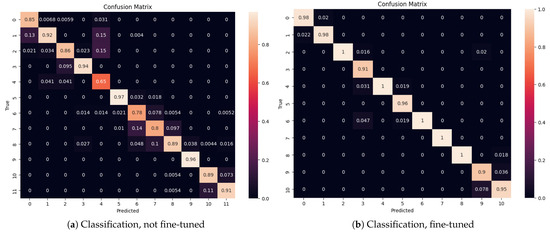
Figure 6.
(a) Confusion matrix for the classification model CNN+LSTM before fine-tuning. (b) Confusion matrix for the classification model CNN+LSTM, fine-tuned with 350 samples per class.
A test was also conducted on the Fine-Tuning Test dataset without fine-tuning, which produced accuracy values below , not shown in the table. The reason for the poor performance of the classifiers when applied, without fine-tuning, to the Fine-Tuning Test dataset was explained in Section 3.2, and it also applies to the regression models.
We then tested the three models in the regression setup on the Pre-Training Test dataset without fine-tuning. Table 3 shows that the CNN+LSTM hybrid model is again the best performer, both in terms of ACPR and mean absolute error (MAE).
Table 3.
Performance of the regression models applied to the Pre-Test dataset (without fine-tuning). Bold text indicates the best accuracy values.
As stated in Section 3.2, the Almost-Correct Prediction Rate (ACPR) is a measure of the percentage of predictions with an Absolute Error smaller than . We show the ACPR performance of the three models with the two thresholds and for the sake of comparability with other works in the literature that only measured the ACPR with [25,44]. Note that the results in Table 3 are only shown for documentation purposes, as they do not represent the objective of this work, which is, instead, to illustrate the performance of the proposed approach with fine-tuning.
The three models were also tested in the regression setup on the Fine-Tuning Test dataset, with fine-tuning and with five increasing per-class cardinalities (100, 200, 350, 500, 700 elements, respectively). In other words, the Test dataset was subsampled in such a way as to obtain five different configurations. In Configuration 1, each class contained 100 elements; in Configuration 2, each class contained 200 elements; etc. As shown in Table 4, increasing the per-class cardinality beyond 350 did not produce significant performance improvements, and according to the ACPR with and MAE, the best performer is again the hybrid CNN+LSTM model.
Table 4.
Performance of the regression models applied to the Fine-Tuning Test dataset (with fine-tuning). The tests were carried out with models fine-tuned with 5 different numbers of samples per class (100, 200, 350, 500, 700) (see text). Bold text indicates the best accuracy values.
Figure 7a,b show the ACPR confusion matrix () for the hybrid CNN+LSTM model, not fine-tuned (a) and fine-tuned (b) with 350 samples per class, evidencing that the performance of the model is nearly uniform across all classes.
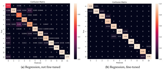
Figure 7.
(a) ACPR confusion matrix () for the regression model CNN+LSTM, not fine-tuned. (b) ACPR confusion matrix () for the regression model CNN+LSTM, fine-tuned with 350 samples per class.
Probably the most interesting feature of regression models is the possibility of predicting, at least in theory, values that were never seen in the fine-tuning step, that is, to interpolate or extrapolate the predicted values. We also tested this characteristic by removing from the Fine-Tuning Training dataset all the samples belonging to classes 0, 2, 3, 4, 6, 7, 8, 10, thus fine-tuning the models only on samples belonging to classes 1, 5, 9. In this case, we compared only the best performers from the previous test, that is, the CNN, LSTM, and CNN+LSTM models. Table 5 reports the ACPR and MAE performance of the models, with the hybrid CNN+LSTM model still clearly winning over the other two.
Table 5.
Performance of the regression models applied to the Fine-Tuning Test dataset (with fine-tuning) trained with 350 samples for the sole classes 1,5,9, that is, the models never met samples from classes 0,2,3,4,6,7,8,10 of the Fine-Tuning dataset before the test.
We consider the results shown above as an important improvement over the state of the art because, to the best of our knowledge, the literature does not report on similar partial fine-tuning. Moreover, the possibility to fine-tune the model on a small subset of the targeted labels, i.e., with only some of the expected occupancies, allows a sensible reduction in fine-tuning time and effort.
6. Conclusions and Further Work
This work presented a passive human counting architecture based on Bluetooth Low Energy (BLE) and a deep neural network model capable of analyzing signal deformations caused by human presence to detect and count occupants in closed indoor environments. Unlike other approaches in the literature, the proposed model is pre-trained on a large dataset and then fine-tuned using a significantly smaller and potentially incomplete dataset acquired directly in the target environment. Experimental results demonstrate that this solution is not only more accurate than state-of-the-art techniques, obtaining a remarkable accuracy value with a fine-tuning on only 350 samples, but also easier to deploy and calibrate, requiring only a few minutes for setup. We believe that this approach can be especially valuable in critical and privacy-sensitive environments such as laboratories, clinics, and hospitals, where camera-based monitoring may be inappropriate or restricted.
The main limitation of the proposed approach is the relatively poor ability to generalize to unseen environments. The principal cause for the need for fine-tuning is the lack of explicit information regarding the structure and geometry of the monitored area, so the model has to learn such information from data. When the monitored area changes, the model needs some form of retraining (for example, fine-tuning) to re-learn such structure.
Future developments of this research will focus on building a generalizable model that eliminates the need for fine-tuning, enabling immediate, privacy-preserving deployment across a wide range of indoor contexts.
Supplementary Materials
The following supporting information can be downloaded at: https://www.mdpi.com/article/10.3390/app15116142/s1.
Author Contributions
Conceptualization, methodology, investigation, formal analysis, writing— original draft preparation, writing—review and editing, G.I. and L.L.B.; investigation, data curation, writing—review and editing, A.N. All authors have read and agreed to the published version of the manuscript.
Funding
This research received no external funding.
Institutional Review Board Statement
Not applicable.
Informed Consent Statement
Not applicable.
Data Availability Statement
The original contributions presented in this study are included in the article/Supplementary Material. Further inquiries can be directed to the corresponding author.
Conflicts of Interest
The authors declare no conflict of interest.
References
- Yang, J.; Pantazaras, A.; Chaturvedi, K.A.; Chandran, A.K.; Santamouris, M.; Lee, S.E.; Tham, K.W. Comparison of different occupancy counting methods for single system-single zone applications. Energy Build. 2018, 172, 221–234. [Google Scholar] [CrossRef]
- Kouyoumdjieva, S.T.; Danielis, P.; Karlsson, G. Survey of Non-Image-Based Approaches for Counting People. IEEE Commun. Surv. Tutor. 2020, 22, 1305–1336. [Google Scholar] [CrossRef]
- Glavin, P.; Bierman, A.; Schieman, S. Private Eyes, They See Your Every Move: Workplace Surveillance and Worker Well-Being. Soc. Curr. 2024, 11, 327–345. [Google Scholar] [CrossRef] [PubMed]
- Liu, J.; Teng, G.; Hong, F. Human Activity Sensing with Wireless Signals: A Survey. Sensors 2020, 20, 1210. [Google Scholar] [CrossRef]
- Youssef, M.; Mah, M.; Agrawala, A. Challenges: Device-Free Passive Localization for Wireless Environments. In Proceedings of the 13th Annual ACM International Conference on Mobile Computing and Networking (MobiCom ’07), Montréal, QC, Canada, 9–14 September 2007; pp. 222–229. [Google Scholar] [CrossRef]
- Iannizzotto, G.; Milici, M.; Nucita, A.; Lo Bello, L. A Perspective on Passive Human Sensing with Bluetooth. Sensors 2022, 22, 3523. [Google Scholar] [CrossRef]
- Li, W.; Vishwakarma, S.; Tang, C.; Woodbridge, K.; Piechocki, R.J.; Chetty, K. Using RF Transmissions From IoT Devices for Occupancy Detection and Activity Recognition. IEEE Sens. J. 2022, 22, 2484–2495. [Google Scholar] [CrossRef]
- Gebru, K.; Rapelli, M.; Rusca, R.; Casetti, C.; Chiasserini, C.F.; Giaccone, P. Edge-based passive crowd monitoring through WiFi Beacons. Comput. Commun. 2022, 192, 163–170. [Google Scholar] [CrossRef]
- Yousaf, J.; Yakoub, S.; Karkanawi, S.; Hassan, T.; Almajali, E.; Zia, H.; Ghazal, M. Through-the-Wall Human Activity Recognition Using Radar Technologies: A Review. IEEE Open J. Antennas Propag. 2024, 5, 1815–1837. [Google Scholar] [CrossRef]
- Laham, S.A.; Baghi, B.H.; Lajoie, P.Y.; Feriani, A.; Herath, S.; Liu, S.; Dudek, G. Device-Free Human State Estimation using UWB Multi-Static Radios. arXiv 2023, arXiv:2401.05410. [Google Scholar]
- Li, C.; Tanghe, E.; Fontaine, J.; Martens, L.; Romme, J.; Singh, G.; De Poorter, E.; Joseph, W. Multistatic UWB Radar-Based Passive Human Tracking Using COTS Devices. IEEE Antennas Wirel. Propag. Lett. 2022, 21, 695–699. [Google Scholar] [CrossRef]
- Nikookar, H.; Prasad, R. UWB Interference. In Introduction to Ultra Wideband for Wireless Communications; Signals and Communication Technology; Springer: Dordrecht, The Netherlands, 2009; pp. 67–92. [Google Scholar] [CrossRef]
- Chen, H.; Zhang, Y.; Li, W.; Tao, X.; Zhang, P. ConFi: Convolutional Neural Networks Based Indoor Wi-Fi Localization Using Channel State Information. IEEE Access 2017, 5, 18066–18074. [Google Scholar] [CrossRef]
- Chen, Z.; Zhang, L.; Jiang, C.; Cao, Z.; Cui, W. WiFi CSI Based Passive Human Activity Recognition Using Attention Based BLSTM. IEEE Trans. Mob. Comput. 2019, 18, 2714–2724. [Google Scholar] [CrossRef]
- Huang, H.; Lin, S. WiDet: Wi-Fi based device-free passive person detection with deep convolutional neural networks. Comput. Commun. 2020, 150, 357–366. [Google Scholar] [CrossRef]
- Chowdary, A.; Bazzi, A.; Chafii, M. On Hybrid Radar Fusion for Integrated Sensing and Communication. IEEE Trans. Wirel. Commun. 2024, 23, 8984–9000. [Google Scholar] [CrossRef]
- Ma, Y.; Zhou, G.; Wang, S. WiFi Sensing with Channel State Information: A Survey. ACM Comput. Surv. 2019, 52, 1–36. [Google Scholar] [CrossRef]
- Soto, J.C.; Galdino, I.; Caballero, E.; Ferreira, V.; Muchaluat-Saade, D.; Albuquerque, C. A survey on vital signs monitoring based on Wi-Fi CSI data. Comput. Commun. 2022, 195, 99–110. [Google Scholar] [CrossRef]
- Qin, Y.; Sigg, S.; Pan, S.; Li, Z. Direction-agnostic gesture recognition system using commercial WiFi devices. Comput. Commun. 2024, 216, 34–44. [Google Scholar] [CrossRef]
- Münch, M.; Huffstadt, K.; Schleif, F. Towards a device-free passive presence detection system with Bluetooth Low Energy beacons. In Proceedings of the 27th European Symposium on Artificial Neural Networks (ESANN 2019), Bruges, Belgium, 24–26 April 2019. [Google Scholar]
- Ramirez, R.; Huang, C.Y.; Liao, C.A.; Lin, P.T.; Lin, H.W.; Liang, S.H. A Practice of BLE RSSI Measurement for Indoor Positioning. Sensors 2021, 21, 5181. [Google Scholar] [CrossRef]
- Billah, M.F.R.M.; Saoda, N.; Gao, J.; Campbell, B. BLE Can See: A Reinforcement Learning Approach for RF-Based Indoor Occupancy Detection. In Proceedings of the 20th International Conference on Information Processing in Sensor Networks (Co-Located with CPS-IoT Week 2021) (IPSN ’21), Nashville, TN, USA, 18–21 May 2021; pp. 132–147. [Google Scholar] [CrossRef]
- Iannizzotto, G.; Lo Bello, L.; Nucita, A. Improving BLE-Based Passive Human Sensing with Deep Learning. Sensors 2023, 23, 2581. [Google Scholar] [CrossRef]
- Münch, M.; Schleif, F.M. Device-Free Passive Human Counting with Bluetooth Low Energy Beacons. In Proceedings of the Advances in Computational Intelligence; Rojas, I., Joya, G., Catala, A., Eds.; Springer: Cham, Switzerland, 2019; pp. 799–810. [Google Scholar] [CrossRef]
- Demrozi, F.; Chiarani, F.; Turetta, C.; Kindt, P.H.; Pravadelli, G. Estimating Indoor Occupancy Through Low-Cost BLE Devices. IEEE Sens. J. 2021, 21, 17053–17063. [Google Scholar] [CrossRef]
- Beato Gutiérrez, M.E.; Sánchez, M.M.; Berjón Gallinas, R.; Fermoso García, A.M. Capacity Control in Indoor Spaces Using Machine Learning Techniques Together with BLE Technology. J. Sens. Actuator Netw. 2021, 10, 35. [Google Scholar] [CrossRef]
- Brockmann, F.; Figura, R.; Handte, M.; Marrón, P.J. RSSI Based Passive Detection of Persons for Waiting Lines Using Bluetooth Low Energy. In Proceedings of the 2018 International Conference on Embedded Wireless Systems and Networks (EWSN ’18), Madrid, Spain, 14–16 February 2018; pp. 102–113. [Google Scholar]
- Feng, C.; Arshad, S.; Liu, Y. MAIS: Multiple Activity Identification System Using Channel State Information of WiFi Signals. In Wireless Algorithms, Systems, and Applications; Ma, L., Khreishah, A., Zhang, Y., Yan, M., Eds.; Springer: Cham, Switzerland, 2017; pp. 419–432. [Google Scholar]
- Adib, F.; Katabi, D. See Through Walls with WiTrack: Device-Free Localization and Tracking Using RF Signals. In Proceedings of the 11th USENIX Symposium on Networked Systems Design and Implementation (NSDI), Seattle, WA, USA, 2–4 April 2014. [Google Scholar]
- Faragher, R.; Harle, R. Location Fingerprinting With Bluetooth Low Energy Beacons. IEEE J. Sel. Areas Commun. 2015, 33, 2418–2428. [Google Scholar] [CrossRef]
- Fink, A.; Beikirch, H.; Voß, M.; Schröder, C. RSSI-based indoor positioning using diversity and Inertial Navigation. In Proceedings of the 2010 International Conference on Indoor Positioning and Indoor Navigation, Zurich, Switzerland, 15–17 September 2010; pp. 1–7. [Google Scholar] [CrossRef]
- Tang, C.; Li, W.; Vishwakarma, S.; Chetty, K.; Julier, S.; Woodbridge, K. Occupancy Detection and People Counting Using WiFi Passive Radar. In Proceedings of the 2020 IEEE Radar Conference (RadarConf20), Florence, Italy, 21–25 September 2020; pp. 1–6. [Google Scholar] [CrossRef]
- Kianoush, S.; Savazzi, S.; Rampa, V.; Nicoli, M. People Counting by Dense WiFi MIMO Networks: Channel Features and Machine Learning Algorithms. Sensors 2019, 19, 3450. [Google Scholar] [CrossRef]
- Huang, J.; Xu, L.; Qian, K.; Wang, J.; Yamanishi, K. Multi-label learning with missing and completely unobserved labels. Data Min. Knowl. Discov. 2021, 35, 1061–1086. [Google Scholar] [CrossRef]
- Zeng, A.; Chen, M.; Zhang, L.; Xu, Q. Are Transformers Effective for Time Series Forecasting? arXiv 2022, arXiv:2205.13504. [Google Scholar] [CrossRef]
- Zhang, G.P. Neural Networks for Time-Series Forecasting. In Handbook of Natural Computing; Rozenberg, G., Bäck, T., Kok, J.N., Eds.; Springer: Berlin/Heidelberg, Germany, 2012; pp. 461–477. [Google Scholar] [CrossRef]
- Zhao, X.; Wang, L.; Zhang, Y.; Han, X.; Deveci, M.; Parmar, M. A review of convolutional neural networks in computer vision. Artif. Intell. Rev. 2024, 57, 99. [Google Scholar] [CrossRef]
- Montesinos López, O.A.; Montesinos López, A.; Crossa, J. Convolutional Neural Networks. In Multivariate Statistical Machine Learning Methods for Genomic Prediction; Springer International Publishing: Cham, Switzerland, 2022; pp. 533–577. [Google Scholar] [CrossRef]
- Van Houdt, G.; Mosquera, C.; Nápoles, G. A review on the long short-term memory model. Artif. Intell. Rev. 2020, 53, 5929–5955. [Google Scholar] [CrossRef]
- Han, C.; Park, H.; Kim, Y.; Gim, G. Hybrid CNN-LSTM Based Time Series Data Prediction Model Study. In Big Data, Cloud Computing, and Data Science Engineering; Lee, R., Ed.; Springer International Publishing: Cham, Switzerland, 2023; pp. 43–54. [Google Scholar] [CrossRef]
- Urbinate, E.; Itano, F.; Del-Moral-Hernandez, E. CNN-LSTM Optimized by Genetic Algorithm in Time Series Forecasting: An Automatic Method to Use Deep Learning. In Artificial Intelligence and Soft Computing; Rutkowski, L., Scherer, R., Korytkowski, M., Pedrycz, W., Tadeusiewicz, R., Zurada, J.M., Eds.; Springer: Cham, Switzerland, 2023; pp. 286–295. [Google Scholar]
- Ahmed, S.; Nielsen, I.E.; Tripathi, A.; Siddiqui, S.; Ramachandran, R.P.; Rasool, G. Transformers in Time-Series Analysis: A Tutorial. Circuits Syst. Signal Process. 2023, 42, 7433–7466. [Google Scholar] [CrossRef]
- Su, L.; Zuo, X.; Li, R.; Wang, X.; Zhao, H.; Huang, B. A systematic review for transformer-based long-term series forecasting. Artif. Intell. Rev. 2025, 58, 80. [Google Scholar] [CrossRef]
- Wang, F.; Zhang, F.; Wu, C.; Wang, B.; Ray Liu, K.J. Passive People Counting using Commodity WiFi. In Proceedings of the 2020 IEEE 6th World Forum on Internet of Things (WF-IoT), New Orleans, LA, USA, 2–16 June 2020; pp. 1–6. [Google Scholar] [CrossRef]
- Nikitin, A.; Iannucci, L.; Kaski, S. TSGM: A Flexible Framework for Generative Modeling of Synthetic Time Series. arXiv 2023, arXiv:2305.11567. [Google Scholar]
- Iwana, B.K.; Uchida, S. Time Series Data Augmentation for Neural Networks by Time Warping with a Discriminative Teacher. In Proceedings of the 2020 25th International Conference on Pattern Recognition (ICPR), Milan, Italy, 10–15 January 2021; pp. 3558–3565. [Google Scholar] [CrossRef]
- Hossin, M.; Sulaiman, M.N. A Review on Evaluation Metrics for Data Classification Evaluations. Int. J. Data Min. Knowl. Manag. Process 2015, 5, 1–11. [Google Scholar] [CrossRef]
- Kazaj, P.M.; Baj, G.; Salimi, Y.; Stark, A.W.; Valenzuela, W.; Siontis, G.C.; Zaidi, H.; Reyes, M.; Graeni, C.; Shiri, I. From Claims to Evidence: A Unified Framework and Critical Analysis of CNN vs. Transformer vs. Mamba in Medical Image Segmentation. arXiv 2025, arXiv:2503.01306. [Google Scholar]
Disclaimer/Publisher’s Note: The statements, opinions and data contained in all publications are solely those of the individual author(s) and contributor(s) and not of MDPI and/or the editor(s). MDPI and/or the editor(s) disclaim responsibility for any injury to people or property resulting from any ideas, methods, instructions or products referred to in the content. |
© 2025 by the authors. Licensee MDPI, Basel, Switzerland. This article is an open access article distributed under the terms and conditions of the Creative Commons Attribution (CC BY) license (https://creativecommons.org/licenses/by/4.0/).