
Kinematic Analysis of an Omnidirectional Tracked Vehicle


Abstract
1. Introduction
2. Materials and Methods
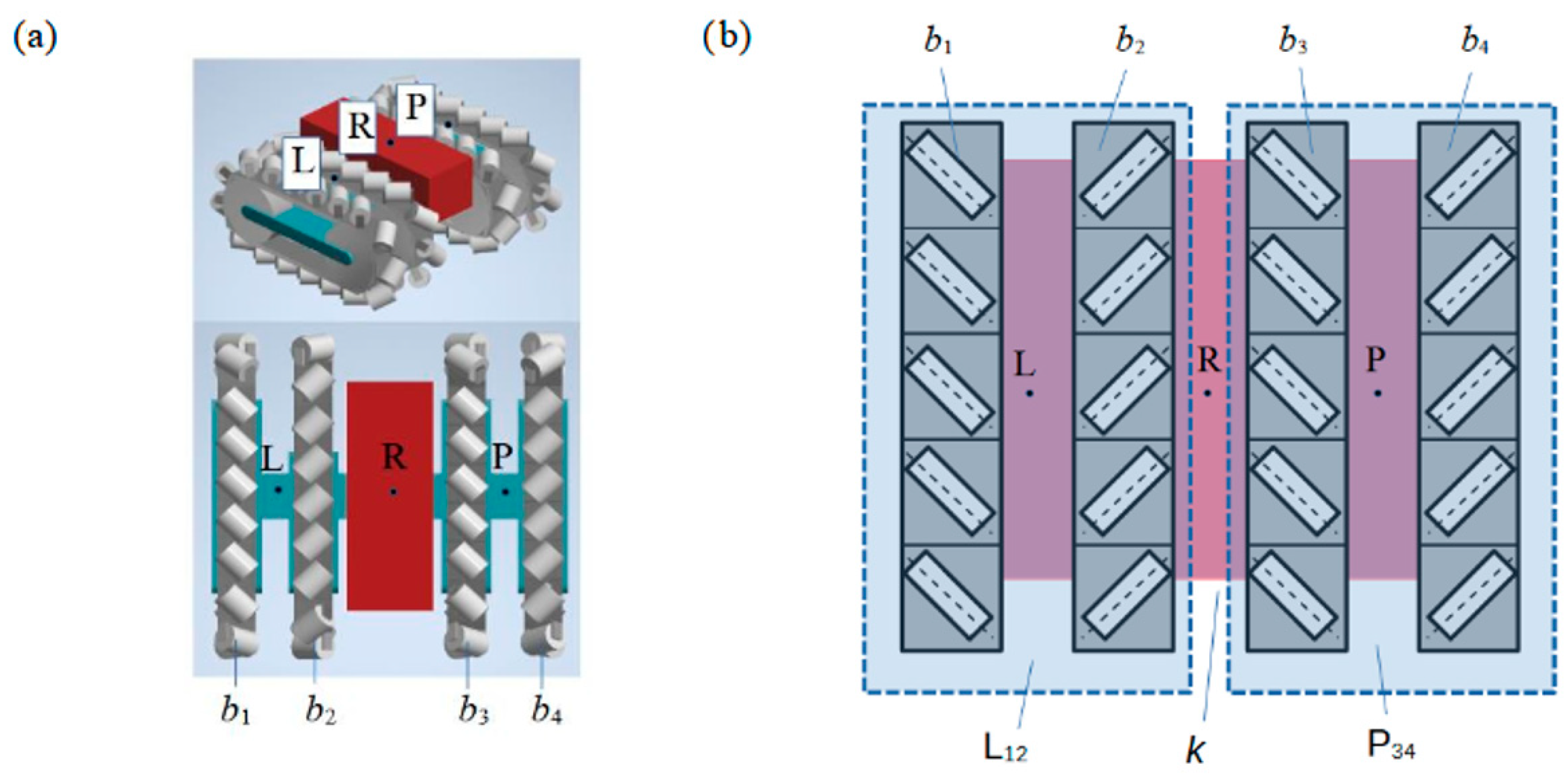
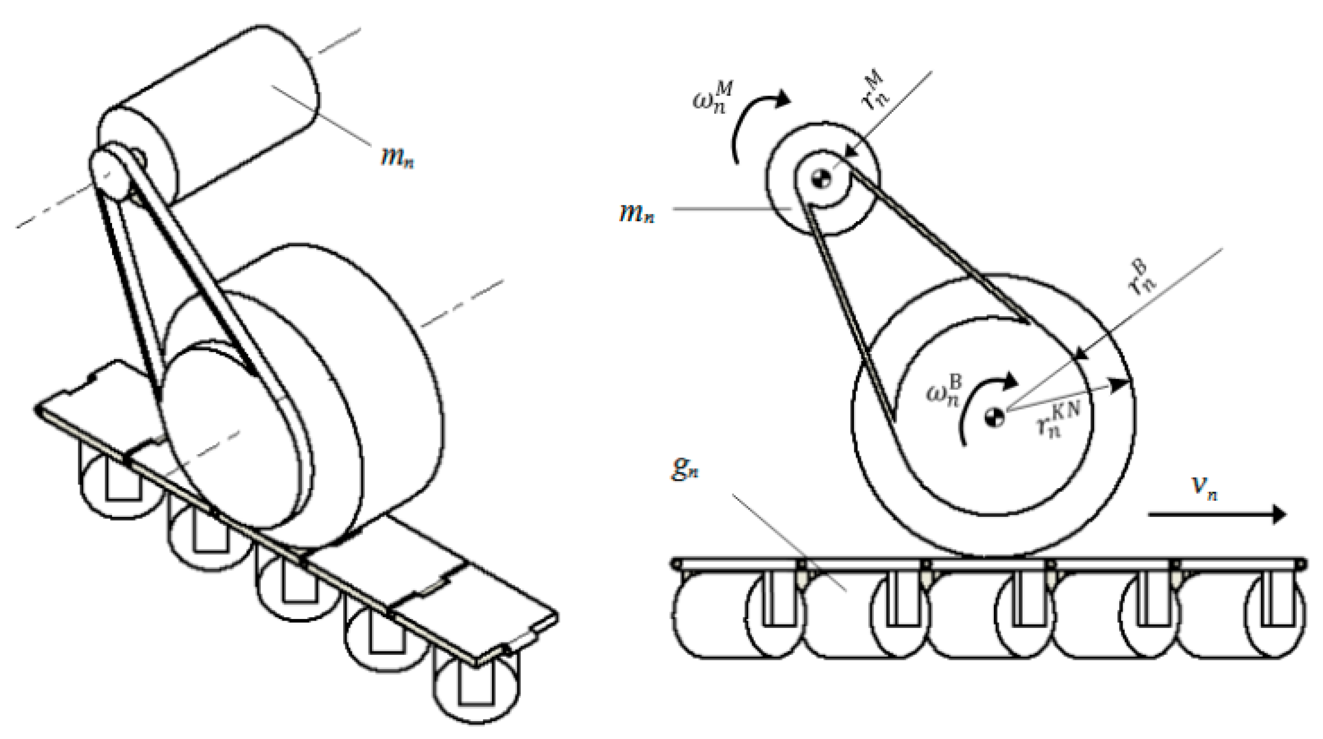
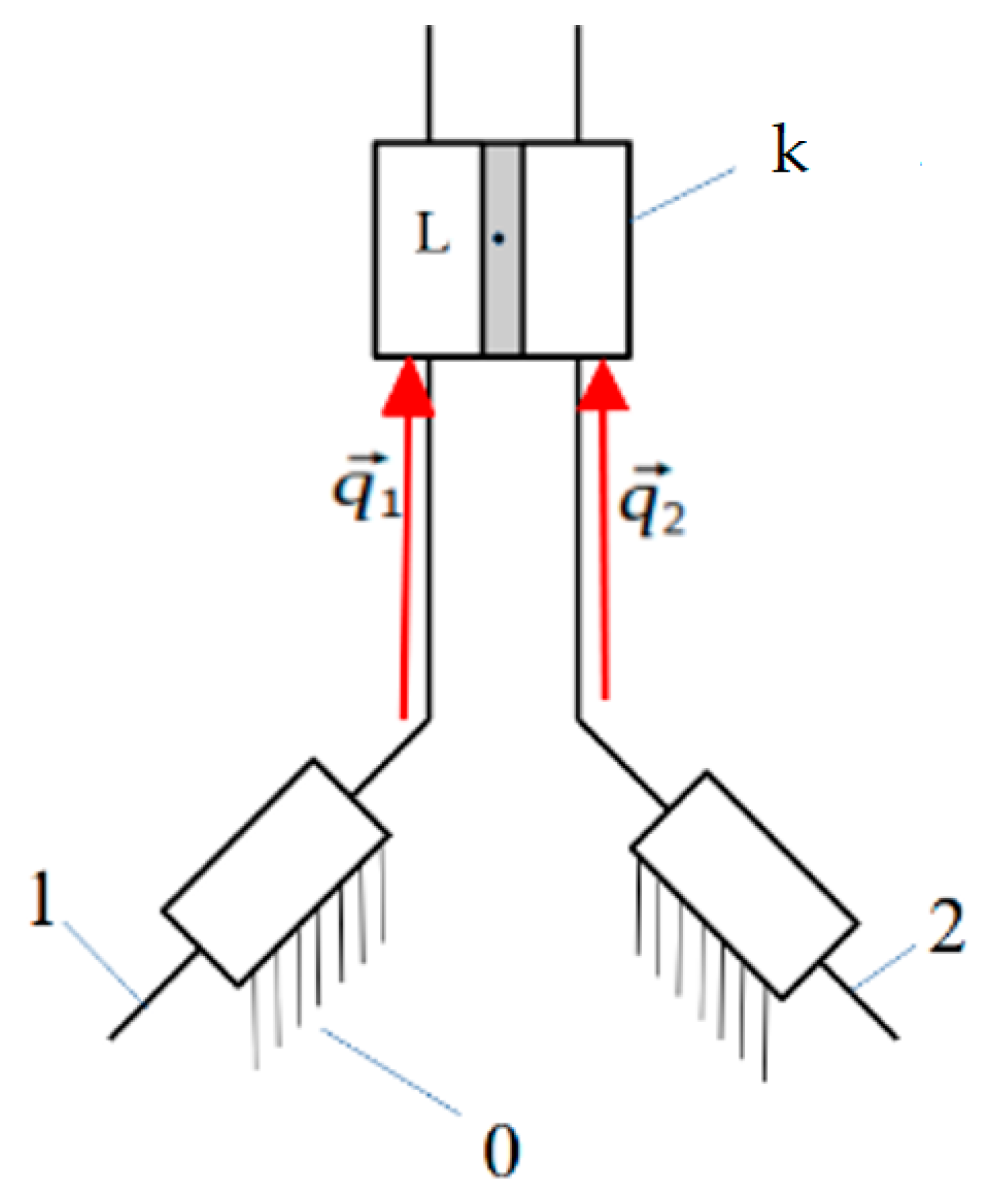
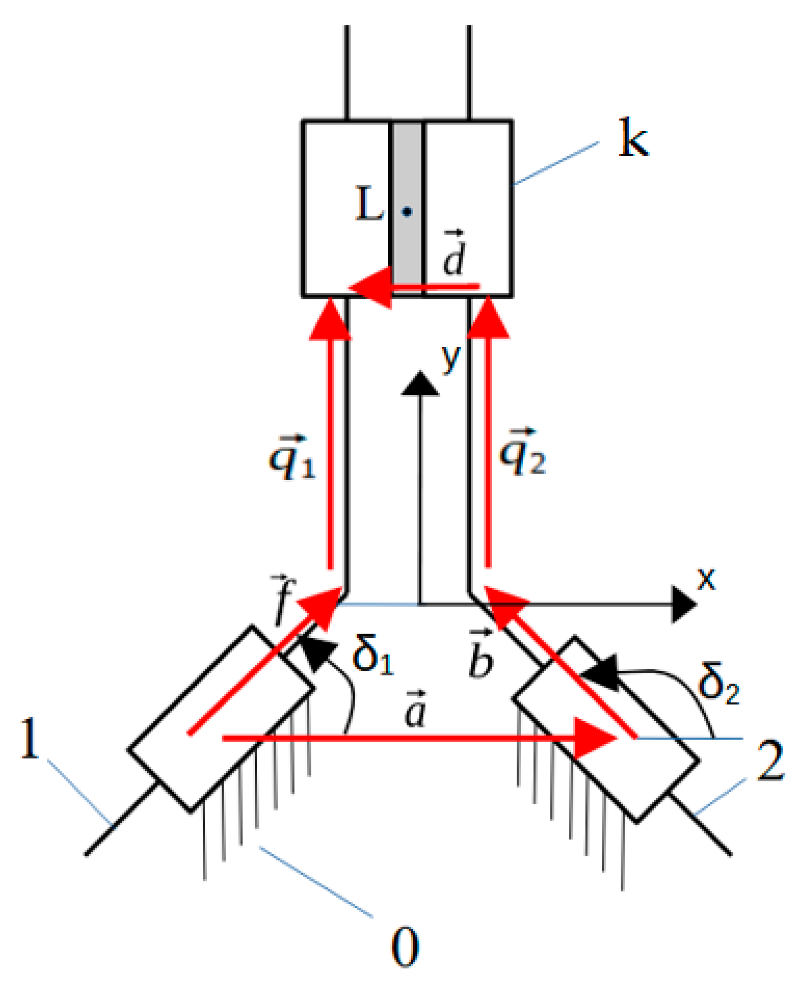
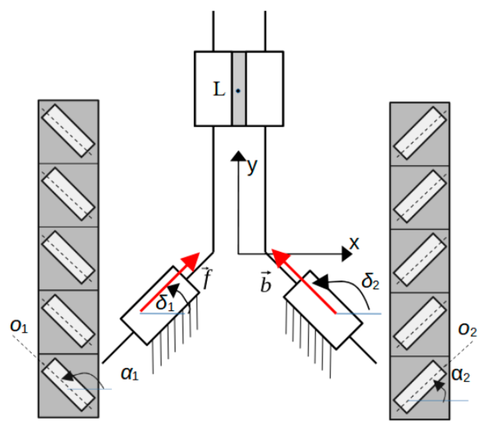
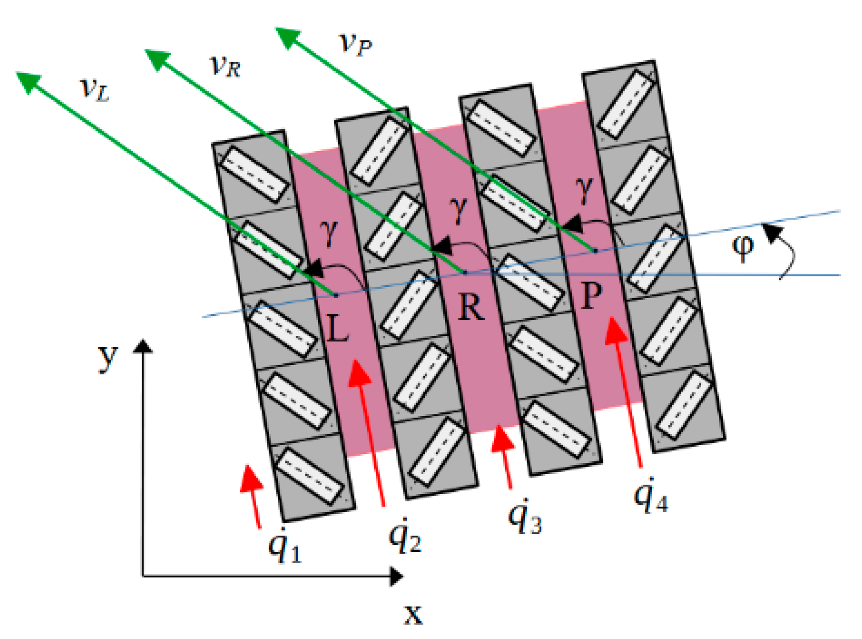
2.1. Kinematic Model
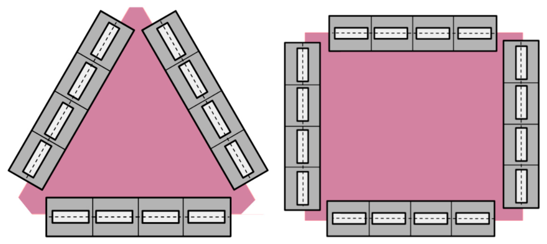
- n—tracked running gear number n = 1, …, 4;
- —radius of the passive wheel of running gear n;
- —radius of the active wheel of running gear n;
- —angular velocity of the passive wheel of running gear n;
- —angular velocity of the active wheel of running gear n.
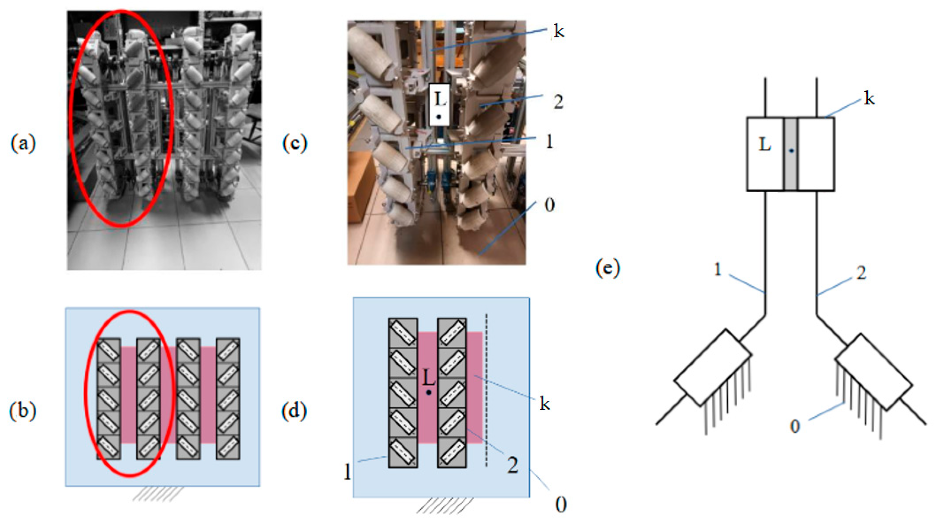
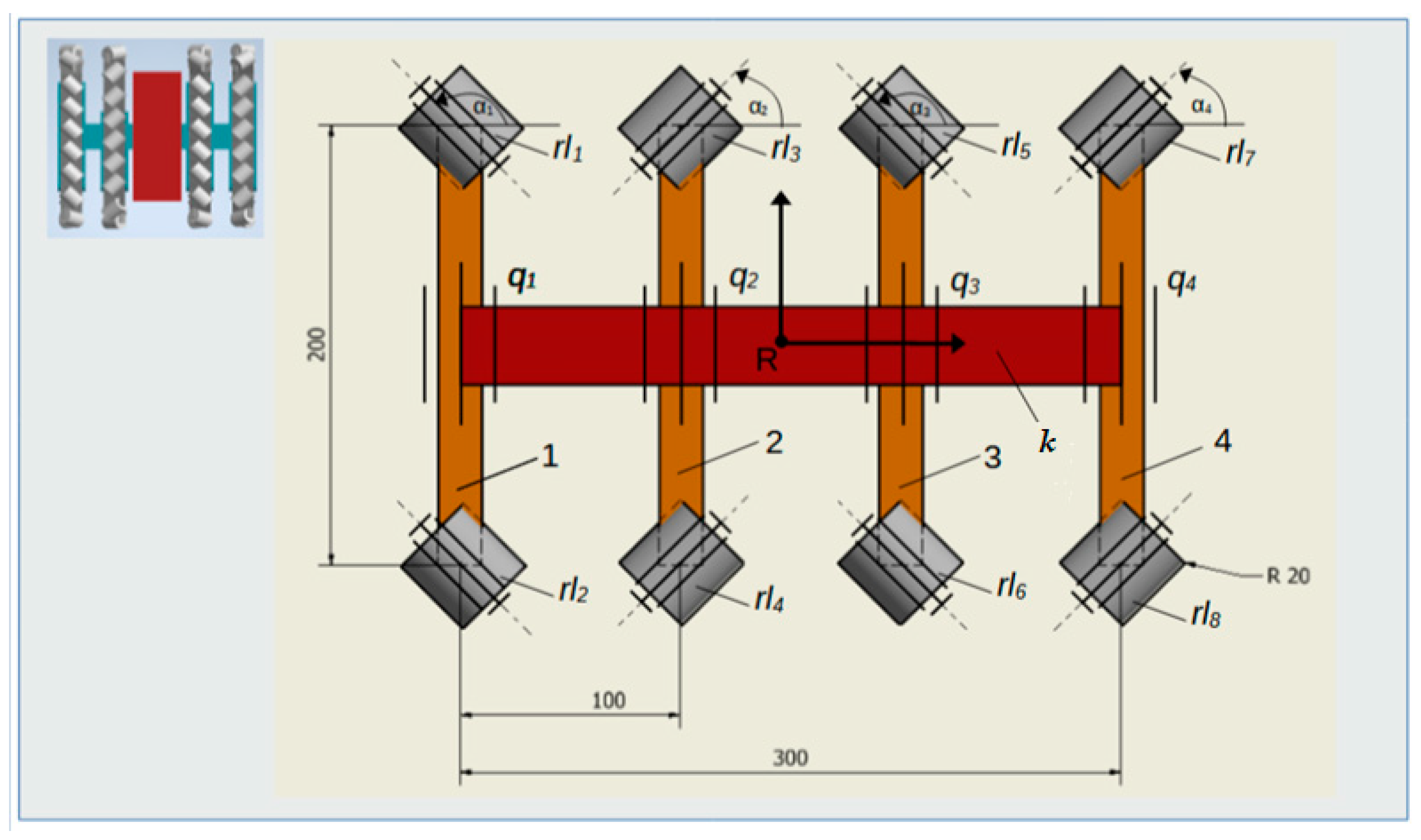
- —mobility;
- —number of bodies;
- —number of pairs of class I.
- For k = 4 and = 4, mobility W is W = 2.
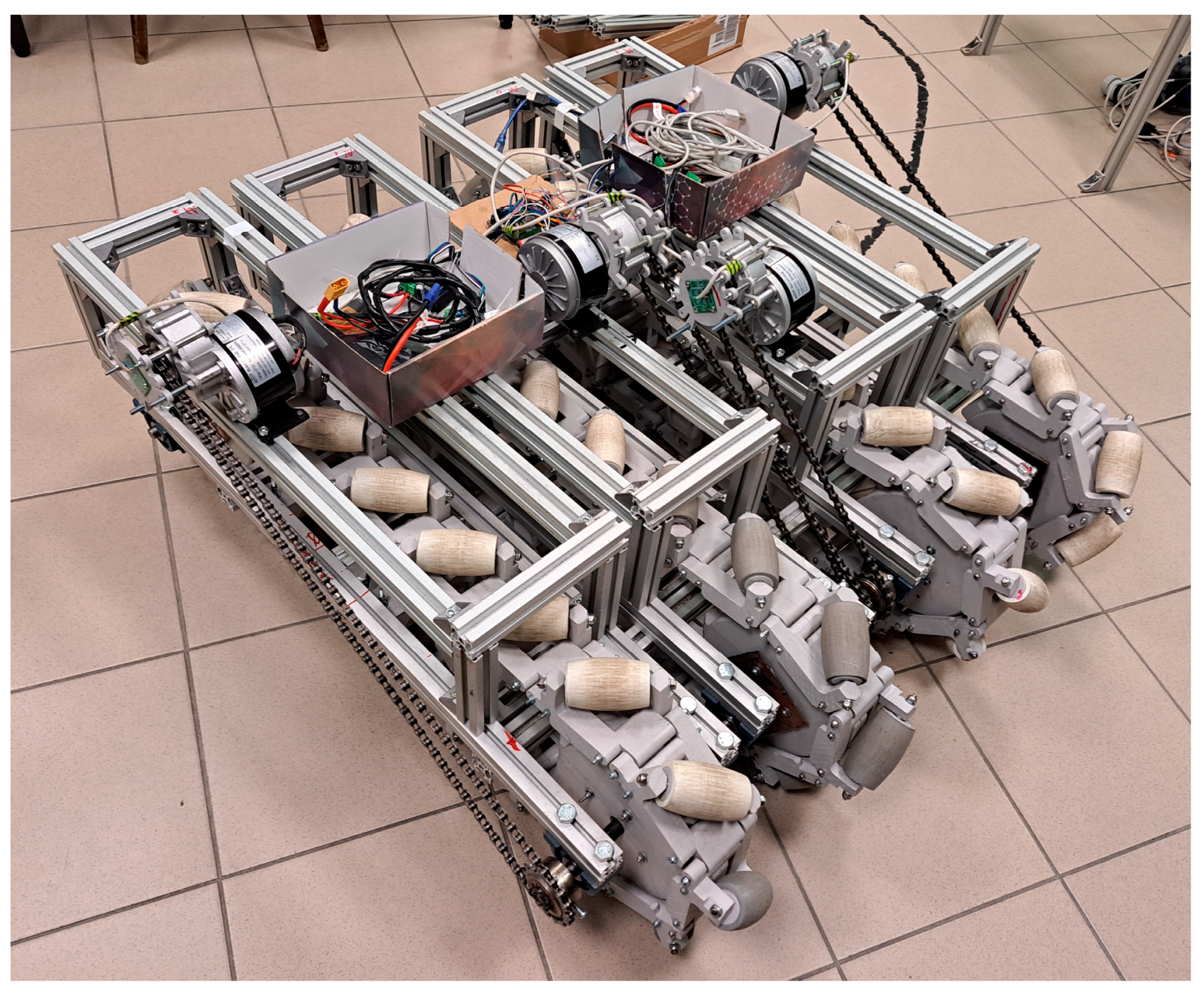
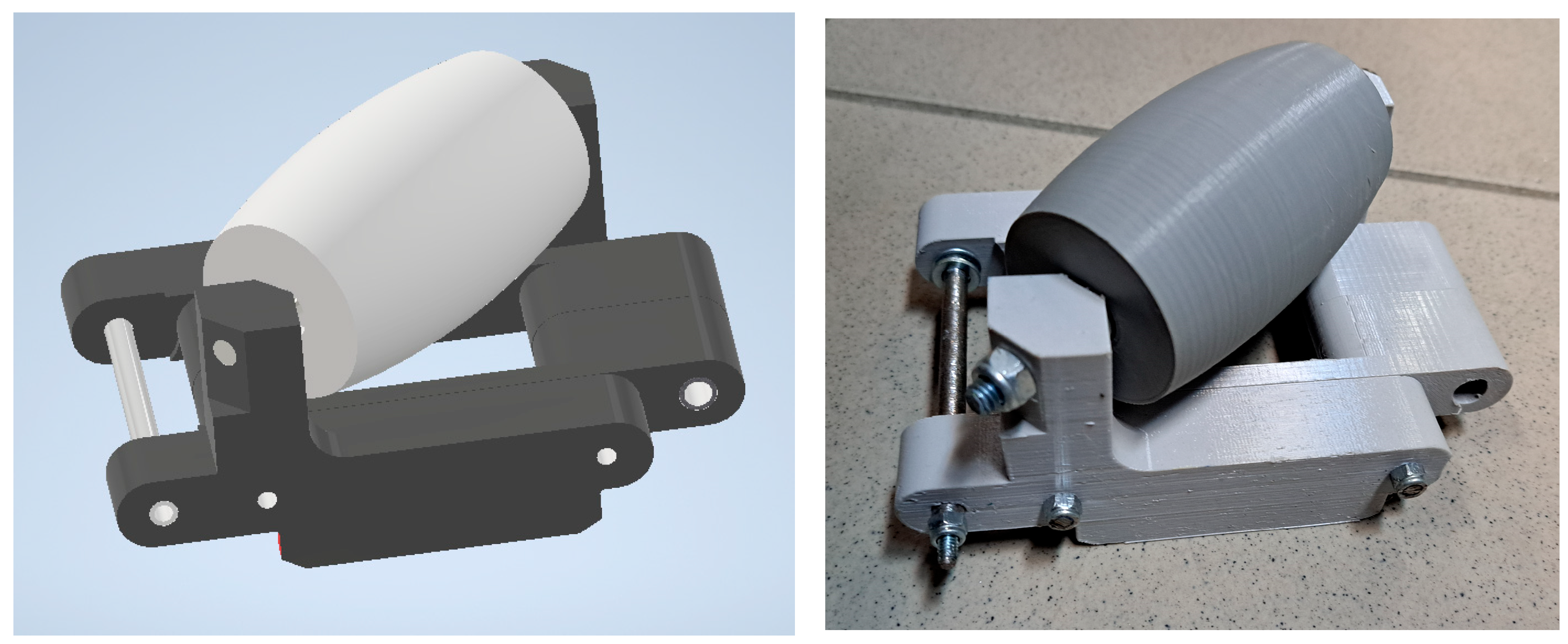
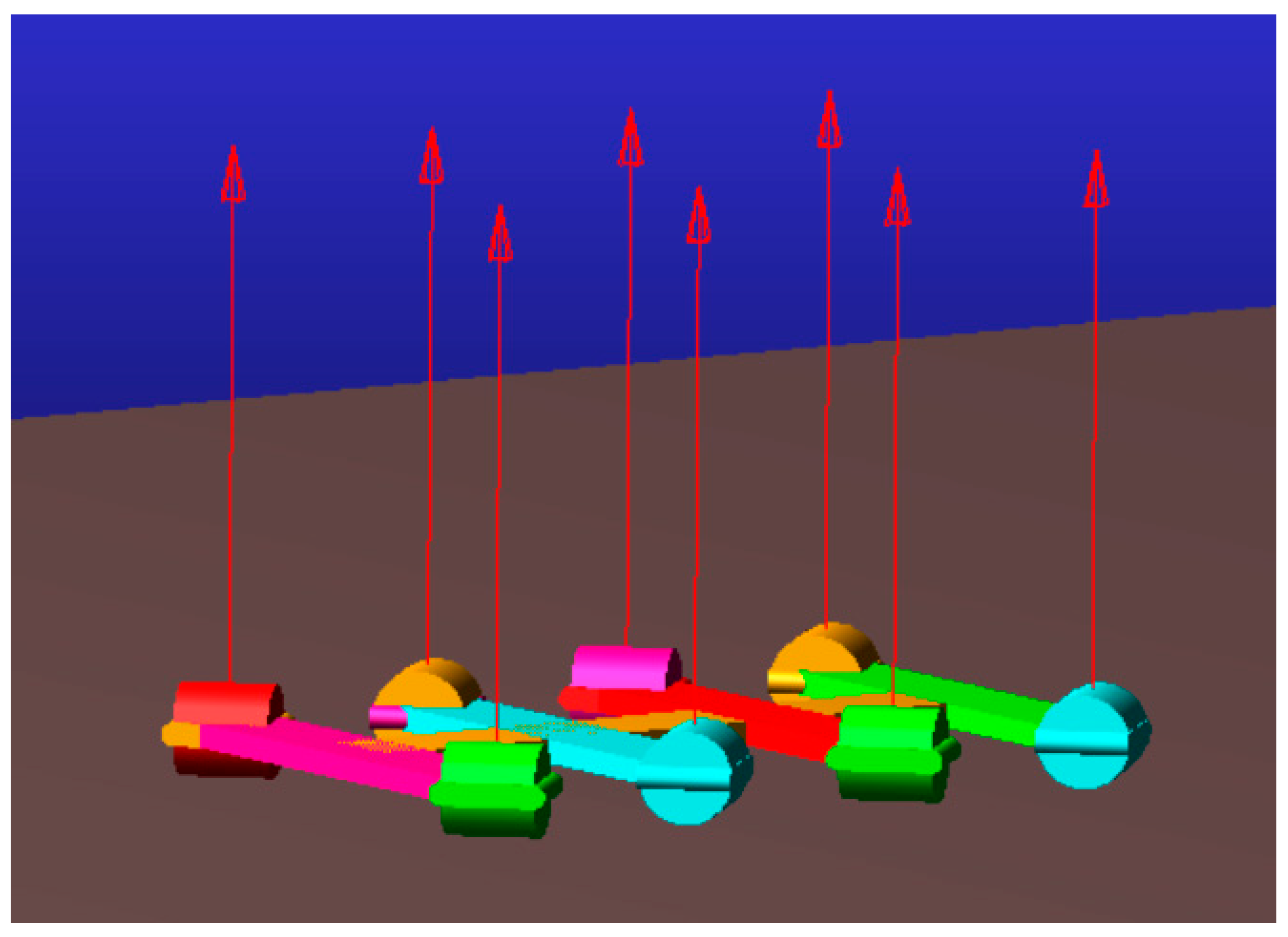
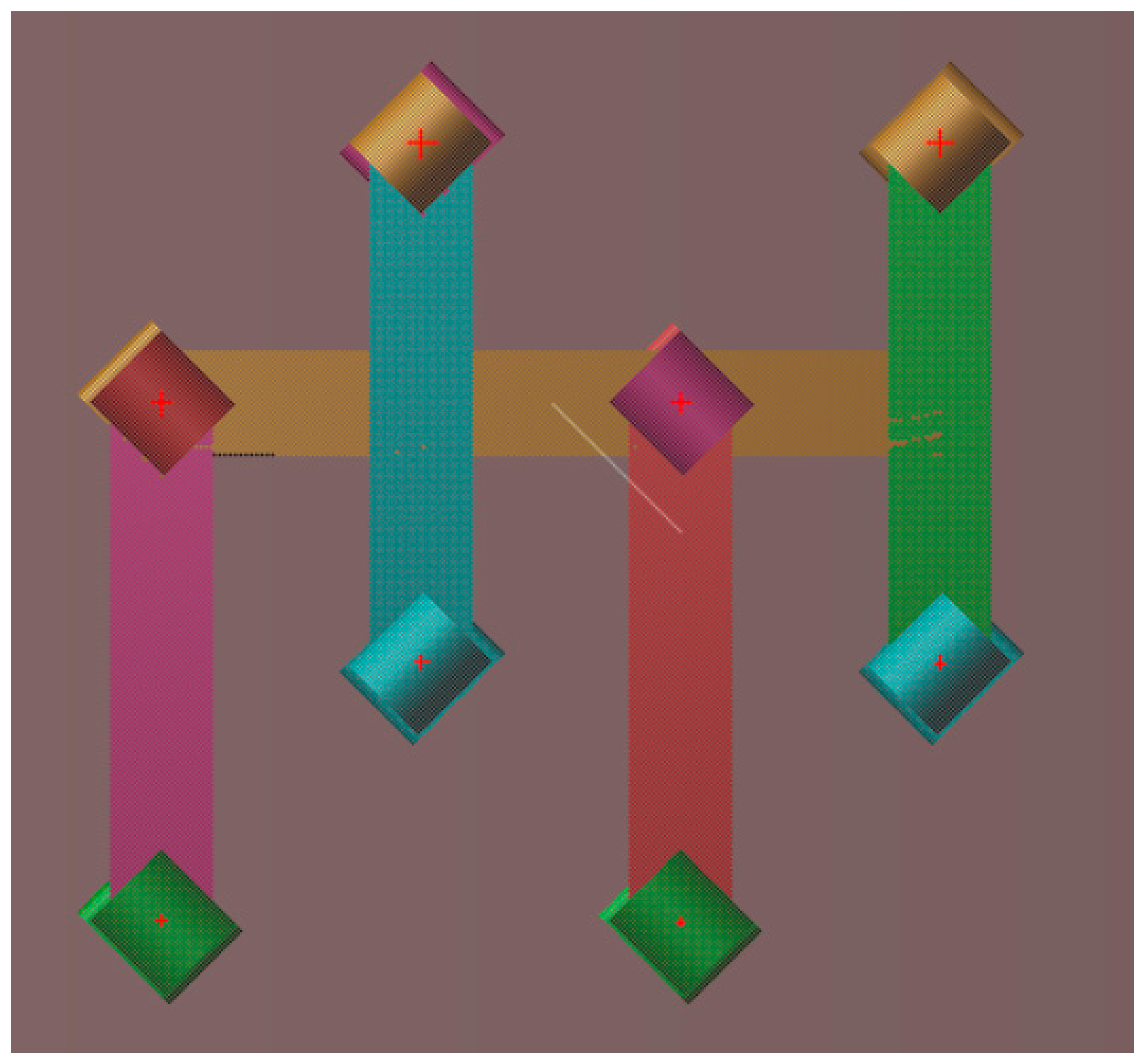
2.2. Simulation Model
2.3. Research Plan
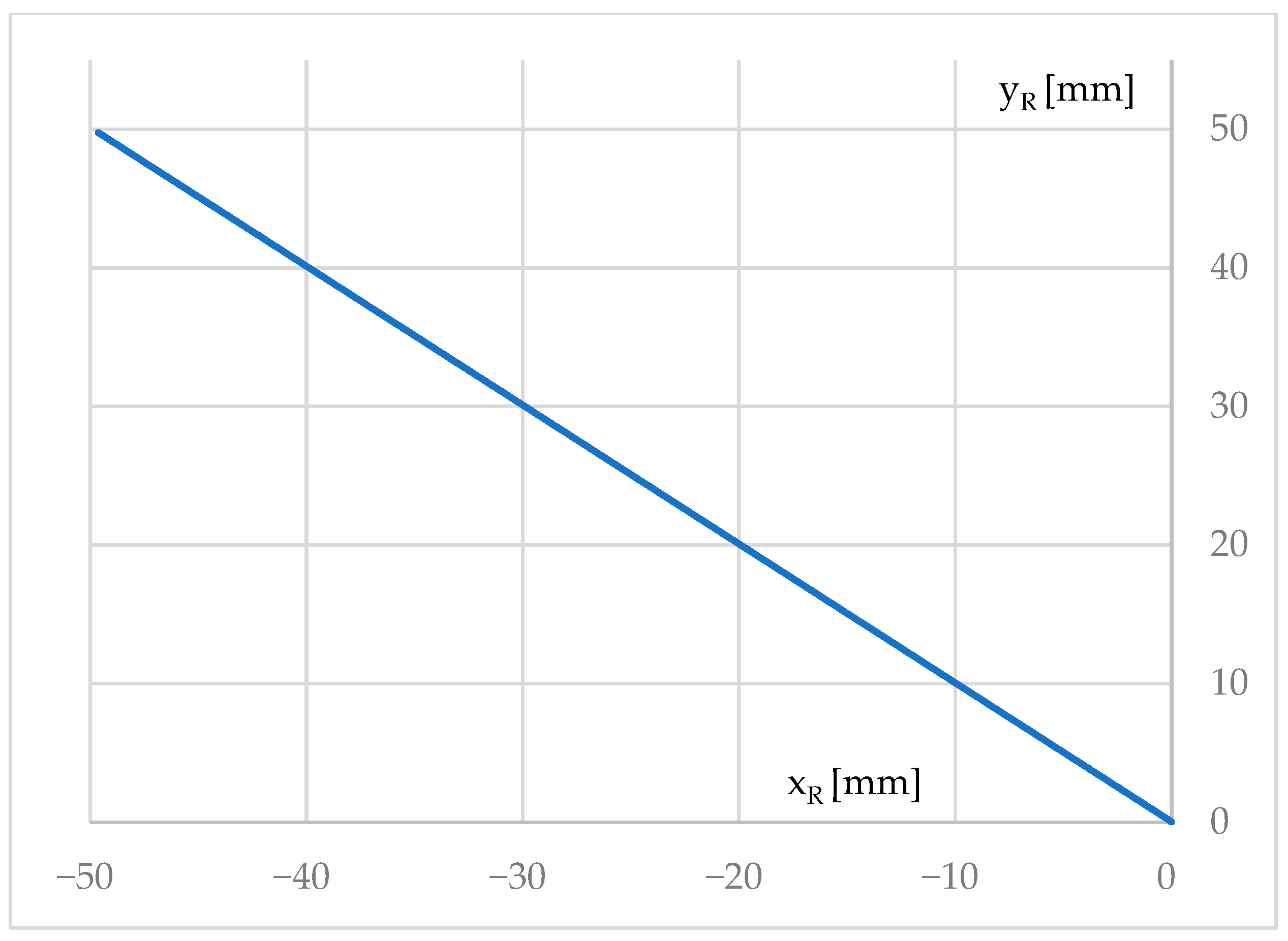
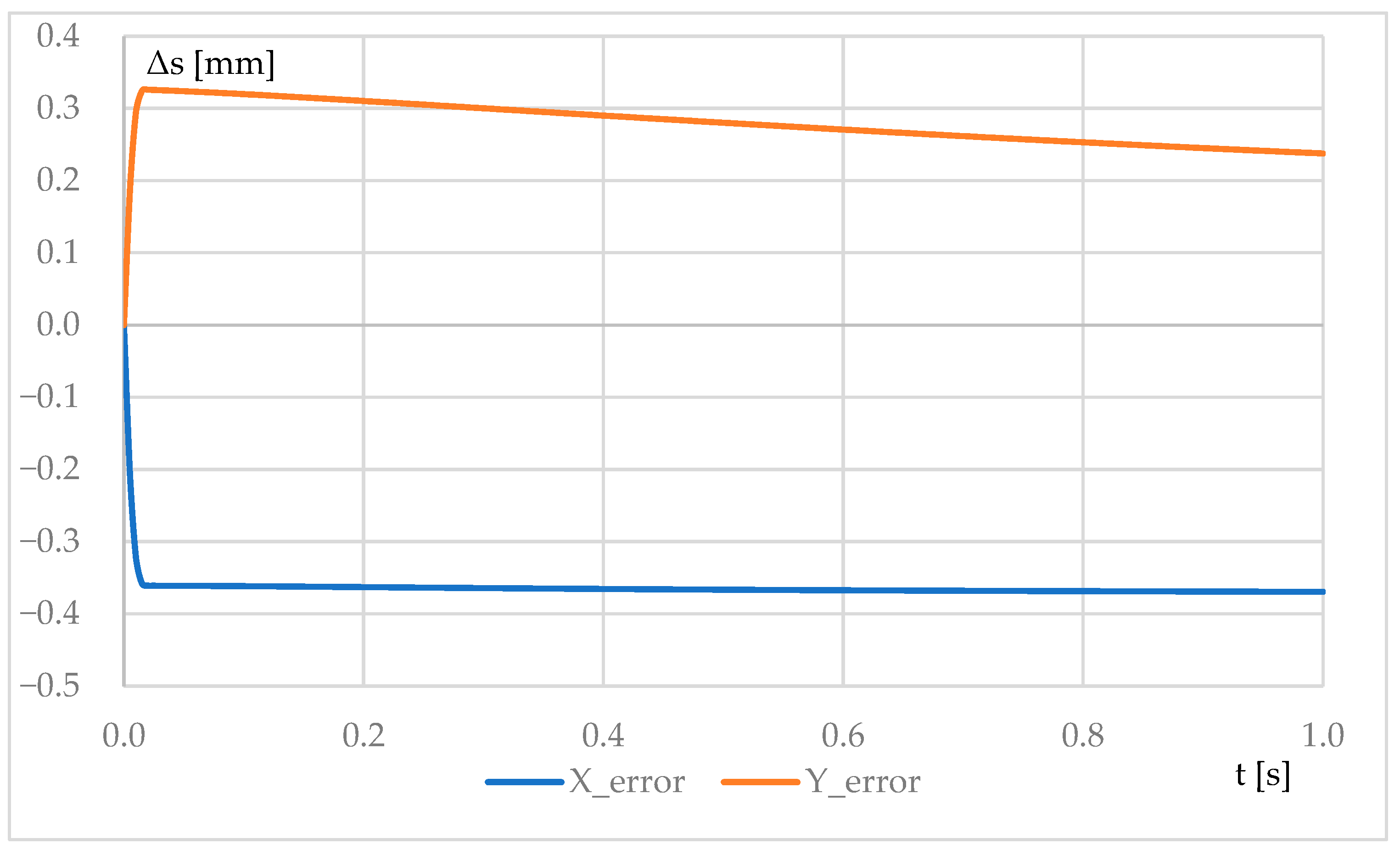
3. Results
4. Discussion
5. Conclusions
Funding
Institutional Review Board Statement
Informed Consent Statement
Data Availability Statement
Conflicts of Interest
References
- Song, J.B.; Byun, K.S. Design and Control of a Four-Wheeled Omnidirectional Mobile Robot with Steerable Omnidirectional Wheels. J. Robot. Syst. 2004, 21, 193–208. [Google Scholar] [CrossRef]
- Watanabe, K. Control of an omnidirectional mobile robot. In Proceedings of the 1998 Second International Conference. Knowledge-Based Intelligent Electronic Systems. Proceedings KES’98 (Cat. No. 98EX111), Adelaide, SA, Australia, 21–23 April 1998; IEEE: New York, NY, USA, 1998; Volume 1, pp. 51–60. [Google Scholar]
- Doroftei, I.; Grosu, V.; Spinu, V. Omnidirectional Mobile Robot Design and Implementation; INTECH Open Access Publisher: London, UK, 2007; pp. 511–528. [Google Scholar]
- Liu, Y.; Zhu, J.J.; Williams, R.L., II; Wu, J. Omni-directional mobile robot controller based on trajectory linearization. Robot. Auton. Syst. 2008, 56, 461–479. [Google Scholar] [CrossRef]
- Grabowiecki, J. Vehicle Wheel. US Patent 1305535, 3 June 1919. [Google Scholar]
- Bae, J.-J.; Kang, N. Design Optimization of a Mecanum Wheel to Reduce Vertical Vibrations by the Consideration of Equivalent, Stiffness. Shock. Vib. 2016, 2016, 5892784. [Google Scholar] [CrossRef]
- Li, Y.; Ge, S.; Dai, S.; Zhao, L.; Yan, X.; Zheng, Y.; Shi, Y. Kinematic Modeling of a Combined System of Multiple Mecanum-Wheeled Robots with Velocity Compensation. Sensors 2019, 20, 75. [Google Scholar] [CrossRef] [PubMed]
- Inhabitat. Available online: https://inhabitat.com/these-omnidirectional-wheels-turn-any-car-into-a-360-degree-maneuvering-machine/ (accessed on 15 March 2025).
- Samarasinghe, S.M. Development and Balancing Control of an Active Omni-Wheeled Unicycle. Ph.D. Dissertation, Asian Institute of Technology, Pathum Thani, Thailand.
- Liddiard, W. Omnidirectional Wheel. US Patent 2016/0023511 A1, 28 January 2016. [Google Scholar]
- Dew Robotics. Available online: http://team1640.com/wiki/index.php/3-Wheel_Swerve (accessed on 15 March 2025).
- Binugroho, E.H.; Setiawan, A.; Sadewa, Y.; Amrulloh, P.H.; Paramasastra, K.; Sudibyo, R.W. Position and Orientation Control of Three Wheels Swerve Drive Mobile RobotPlatform. In Proceedings of the 2021 International Electronics Symposium (IES), Surabaya, Indonesia, 29–30 September 2021; pp. 669–674. [Google Scholar]
- Park, K.P.; Ham, S.H.; Lee, W.Y.; Yoo, B.W. Development of transporter trainingsimulator based on virtual reality and vehicle dynamics model. Int. J. Nav. Archit. Ocean. Eng. 2023, 15, 100547. [Google Scholar] [CrossRef]
- Tadakuma, K.; Takane, E.; Fujita, M.; Nomura, A.; Komatsu, H.; Konyo, M.; Tadokoro, S. Planar omnidirectional crawler mobile mechanism—Development of actual mechanicalprototype and basic experiments. IEEE Robot. Autom. Lett. 2017, 3, 395–402. [Google Scholar]
- Takane, E.; Tadakuma, K.; Shimizu, T.; Hayashi, S.; Watanabe, M.; Kagami, S.; Nagatani, K.; Konyo, M.; Tadokoro, S. Basic Performance of Planar Omnidirectional Crawler During Direction Switching Using Disturbance Degree of Ground Evaluation Method. In Proceedings of the 2019 IEEE/RSJ InternationalConference on Intelligent Robots and Systems (IROS), Macau, China, 3–8 November 2019; pp. 2732–2739. [Google Scholar]
- Isoda, T.; Chen, P.; Mitsutake, S.; Toyota, T. Roller-Crawler Type of Omni-Directional Mobile Robot for Off-Road Running. Trans. Jpn. Soc. Mech. Eng. Ser. C 1999, 65, 3282–3289. [Google Scholar] [CrossRef]
- Blog Arduino. Available online: https://blog.arduino.cc/2023/02/22/james-bruton-improves-his-triangle-tracked-tank/ (accessed on 16 January 2024).
- Chen, P.; Mitsutake, S.; Isoda, T.; Shi, T. Omni-directional robot and adaptive control method for off-road running. IEEE Trans. Robot. Autom. 2002, 18, 251–256. [Google Scholar] [CrossRef]
- Raj, L.; Czmerk, A. Modelling and simulation of the drivetrain of an omnidirectional mobile robot. Automatika Časopis Autom. Mjer. Elektron. Računarstvo Komunikacije 2017, 58, 232–243. [Google Scholar] [CrossRef]
- Zhang, Y.; Yang, H.; Fang, Y. Design and motion analysis of a novel track platform. J. Phys. Conf. Ser. 2018, 1074, 012014. [Google Scholar] [CrossRef]
- Zhang, Y.; Huang, T. Research on a tracked omnidirectional and cross-country vehicle. Mech. Mach. Theory 2015, 87, 18–44. [Google Scholar] [CrossRef]
- Hoppe, N.; Kuznetsov, I.; Uriarte, C.; Freitag, M. A New Omnidirectional Track Drive System for Off-Road Vehicles. In Proceedings of the XXII International Conference on “Material Handling, Constructions and Logistics”, Belgrade, Serbia, 4–6 October 2017. [Google Scholar]
- Fang, Y.; Zhang, Y.; Li, N.; Shang, Y. Research on a medium-tracked omni-vehicle. Mech. Sci. 2020, 11, 137–152. [Google Scholar] [CrossRef]
- Fang, Y.; Zhang, Y.; Shang, Y.; Huang, T.; Yan, M. Center-point steering analysis of tracked omni-vehicles based on skid conditions. Mech. Sci. 2021, 12, 511–527. [Google Scholar] [CrossRef]
- Fiedeń, M.; Bałchanowski, J. A Mobile Robot with Omnidirectional Tracks—Design and Experimental Research. Appl. Sci. 2021, 11, 11778. [Google Scholar] [CrossRef]
- Fiedeń, M.; Bałchanowski, J. Simulation studies and experimental research of omnidirectional tracked vehicle. J. Theor. Appl. Mech. 2024, 62, 14292955. [Google Scholar] [CrossRef] [PubMed]
- Rijalusalam, D.U.; Iswanto, I. Implementation kinematics modeling and odometry of four omni wheel mobile robot on the trajectory planning and motion control based microcontroller. J. Robot. Control 2021, 2, 448–455. [Google Scholar] [CrossRef]
- Tlale, N.; de Villiers, M. Kinematics and dynamics modelling of a mecanum wheeled mobile platform. In Proceedings of the 2008 15th International Conference on Mechatronics and Machine Vision in Practice, Auckland, New Zealand, 2–4 December 2008; pp. 657–662. [Google Scholar]
- Yan, X.; Wang, S.; He, Y.; Ma, A.; Zhao, S. Autonomous Tracked Vehicle Trajectory Tracking Control Based on Disturbance Observation and Sliding Mode Control. Actuators 2025, 14, 51. [Google Scholar] [CrossRef]
- Miller, S. Teoria Maszyn i Mechanizmów: Analiza Układów Kinematycznych; Oficyna Wydawnicza Politechniki Wrocławskiej: Wrocław, Poland, 1996. [Google Scholar]
- Gronowicz, A. Podstawy Analizy Układów Kinematycznych; Oficyna Wydawnicza Politechniki Wrocławskiej: Wrocław, Poland, 2003. [Google Scholar]
- Ben Hazem, Z.; Guler, N.; Altaif, A.H. A study of advanced mathematical modeling and adaptive control strategies for trajectory tracking in the Mitsubishi RV-2AJ 5-DOF Robotic Arm. Discov. Robot. 2025, 1, 2. [Google Scholar] [CrossRef]
- Engström, J.; Richloow, E.; Wickström, A. Modeling of Robotic Hand for Dynamic Simulation. Bachelor’s Thesis, School of Industrial Engineering and Management (ITM), Stockholm, Sweden, 2010. MMKB 2010:23. [Google Scholar]
- Pasini, D. Modelling of Mobile Vehicles for Simulation and Control. Master’s Thesis, Politecnico di Torino, Torino, Italy, 2019. [Google Scholar]
- Wikipedia. Available online: https://pl.wikipedia.org/wiki/Wsp%C3%B3%C5%82czynnik_tarcia (accessed on 4 March 2024).


| Stiffness | 20 N/mm | Static Coefficient | 1 |
| Force Exponent | 2.2 | Dynamic Coefficient | 0.85 |
| Damping | 1 Ns/mm | Stiction Transition Velocity | 10 mm/s |
| Penetration Depth | 1 mm | Friction Transition Velocity | 2000 mm/s |
| ID | [m/s] | [m/s] | [m/s] | [m/s] | [m/s] |
|---|---|---|---|---|---|
| 1 | 100 | −100 | −100 | ||
| 2 | 100 | 0 | |||
| 3 | 100 | 50 |
| ID | [m/s] | [m/s] | [m/s] | [m/s] | [m/s] |
|---|---|---|---|---|---|
| 4 | 100 | −100 | 200 | −200 | |
| 5 | 100 | 0 | 100 | −100 | 100 |
| 6 | 100 | 50 | 50 | −50 |
| ID | [m/s] | [m/s] | [m/s] | [m/s] | [m/s] |
|---|---|---|---|---|---|
| 7 | 100 | −100 | ~129.8 | ||
| 8 | 100 | 0 | ~89.8 | ||
| 9 | 100 | 50 | ~87.6 |
| ID | [mm] | [mm] | [mm] | [mm] | Δex [mm] | Δey [mm] | Δe [mm] | e [%] |
|---|---|---|---|---|---|---|---|---|
| 1 | −99.07 | 0.34 | −100 | 0 | −0.93 | −0.34 | 0.99 | 0.99 |
| 2 | −49.63 | 49.76 | −50 | 50 | −0.37 | 0.24 | 0.44 | 0.62 |
| 3 | −24.72 | 74.75 | −25 | 75 | −0.28 | 0.25 | 0.38 | 0.47 |
| 4 | −169.15 | 1.83 | −173.2 | 0 | −4.05 | −1.83 | 4.44 | 2.57 |
| 5 | −85.38 | 49.78 | −86.6 | 50 | −1.22 | 0.22 | 1.24 | 1.24 |
| 6 | −42.71 | 74.81 | −43.3 | 75 | 0.59 | 0.19 | 0.62 | 0.72 |
| 7 | −126.64 | 27.22 | −126.79 | 26.79 | −0.15 | −0.57 | 0.59 | 0.46 |
| 8 | −62.72 | 62.99 | −63.4 | 63.4 | 0.68 | 0.41 | 0.79 | 0.88 |
| 9 | −31.25 | 81.38 | −31.7 | 81.7 | −0.45 | 0.32 | 0.55 | 0.63 |
| mn [kg] | [mm] | [mm] | [mm] | [mm] | Δex [mm] | Δey [mm] | Δe [mm] | e [%] |
|---|---|---|---|---|---|---|---|---|
| 60 | −99.04 | 0.35 | −100 | 0 | −0.96 | −0.35 | 1.02 | 1.02 |
| 80 | −99.06 | 0.34 | −100 | 0 | −0.94 | −0.34 | 1.00 | 1.00 |
| 100 | −99.07 | 0.34 | −100 | 0 | −0.93 | −0.34 | 0.99 | 0.99 |
| 120 | −99.08 | 0.33 | −100 | 0 | −0.92 | −0.33 | 0.98 | 0.98 |
Disclaimer/Publisher’s Note: The statements, opinions and data contained in all publications are solely those of the individual author(s) and contributor(s) and not of MDPI and/or the editor(s). MDPI and/or the editor(s) disclaim responsibility for any injury to people or property resulting from any ideas, methods, instructions or products referred to in the content. |
© 2025 by the author. Licensee MDPI, Basel, Switzerland. This article is an open access article distributed under the terms and conditions of the Creative Commons Attribution (CC BY) license (https://creativecommons.org/licenses/by/4.0/).
Share and Cite
Fiedeń, M. Kinematic Analysis of an Omnidirectional Tracked Vehicle. Appl. Sci. 2025, 15, 6111. https://doi.org/10.3390/app15116111
Fiedeń M. Kinematic Analysis of an Omnidirectional Tracked Vehicle. Applied Sciences. 2025; 15(11):6111. https://doi.org/10.3390/app15116111
Chicago/Turabian StyleFiedeń, Mateusz. 2025. "Kinematic Analysis of an Omnidirectional Tracked Vehicle" Applied Sciences 15, no. 11: 6111. https://doi.org/10.3390/app15116111
APA StyleFiedeń, M. (2025). Kinematic Analysis of an Omnidirectional Tracked Vehicle. Applied Sciences, 15(11), 6111. https://doi.org/10.3390/app15116111