1. Introduction
Automated Guided Vehicles (AGVs) are self-navigating systems that operate through a combination of onboard sensors and software algorithms [
1]. They can follow paths using a variety of approaches, including laser triangulation, magnetic tapes, grids, wires, and optical guidance. These vehicles do not require a driver or operator, making them ideal for automating repetitive transport tasks in structured environments [
1].
The first credited commercially available AGV dates back to 1954 when Arthur Barrett modified a tow truck so that it followed a wire on the floor. He named his invention “
Guide-O-Matic” and it was offered by his company Barrett Electronics [
1]. Back then, AGV applications were limited by the available sensors and computers, but nowadays, AGVs are widely used in manufacturing applications, due to their practicality and autonomous operation in dynamic environments [
2]. Examples of current AGV applications include transport systems in warehouses and container terminals [
3], and crop height measurement in the agricultural field [
4].
In contrast, Autonomous Mobile Robots (AMRs) can perceive and interpret their environment, enabling them to navigate more flexibly than AGVs [
5]. Unlike AGVs, which rely on fixed guidance infrastructure, AMRs build a virtual model of their surroundings to localize and plan navigation paths dynamically. Under this approach, the system creates a path plan to follow, instead of relying on external guidance like AGVs [
6]. Due to their level of autonomy, these systems can transport material (similarly to AGVs), and perform more complex tasks such as surveillance and human–robot collaboration (e.g., with operators) [
2].
In the 1990’s, many control and navigation methods were implemented in AMR systems. For instance, a navigation method based on estimating a path using a sensed environment was proposed in [
7]. Static and moving obstacle avoidance has also been influenced by Fuzzy control [
8], which has excelled by facilitating the implementation of heuristic control, being stable, and providing easy implementation [
9]. Other improvements have focused on controlling various AMR systems at the same time, which are hierarchically organized using a traffic control [
10]. Advanced approaches in the AGV field have allowed significant improvements in precision in applications that previously were impossible, e.g., Shijian et al. [
11] proposed the use of magnetic tracks to increase AGV position accuracy, reducing the error from ±5 mm to ±1.69 mm. This improvement has allowed the implementation of AGV systems in some industrial applications that require almost millimeter precision, such as navigating narrow aisles in a warehouse.
In recent years, the development of complex AMR systems has increased. Gatesichapakorn et al. [
12] developed a system running a Robot Operating System (ROS), a 2D LiDAR, and an RGB-D camera. In this work, two robot configurations were used to evaluate the performance in avoiding obstacles in an indoor environment with public space and a narrow way, one running on a Raspberry Pi 3 and a 2D LiDAR, and the other consisting of an Intel NUC, a 2D LiDAR, and an RGB-D camera. Iqbal et al. [
4] presented a mobile field robot running ROS and a 2D LiDAR to navigate an occluded crop; the proposed navigation strategy based on a nodding LiDAR configuration achieved similar results to commonly used LiDAR configurations. Recent works have integrated reinforcement learning to enhance adaptive navigation and velocity control in AMRs [
13]. Others have employed deep Q-learning with transfer learning for robust path planning in dynamic settings [
14].
In 2020, due to the SARS COVID-19 pandemic, the idea of using AGVs for hospital applications began to spread widely. The vehicle’s tasks could include monitoring of patients’ health parameters such as oxygenation level, temperature, and heart rate; transportation of medicine from nurses to patients; and the disposal of waste material. One AGV implementation in this context was based on an infrared sensor to follow a wire on the floor and an ultrasonic sensor to avoid collisions [
15]. Such implementations demonstrated how functional an AGV system could be when physical contact between people must be avoided, such as in hospital settings. When the first SARS COVID-19 cases started to appear on the American continent in early 2020 [
16], several universities around the world took early actions to minimize the risk of propagation among students and collaborators of the university. The first step was to cancel onsite classes and migrate to an online model for academic continuity in early 2020; furthermore, some universities such as Tecnologico de Monterrey started to develop service robots as surveillance systems for social distancing [
17].
Other universities around the world implemented similar AMR systems focused on surveillance of aspects such as social distancing, the use of hand sanitizer, and the correct use of face masks. For example, the University of Maryland surveyed social distance maintenance with the help of a 2D LiDAR, an RGB-D camera, and closed-circuit television (CCTV) [
18]. The Ricardo Palma University in Peru designed a 3-wheeled robot with two anthropomorphic hands to detect face masks with AI trained cameras, dispense hand sanitizer, and monitor vital signs called “
ROHNI-1” [
19]. The Handong Global University in Korea designed a contactless office-assistant service robot capable of using image recognition, user tracking, and voice recognition to offer automated assistive service to students and staff at the university’s campus [
20]. While these academic institutions developed successful designs, there are certain limitations that constrain their practical feasibility. Many of these solutions remain at the conceptual stage, lack autonomy capability, or offer simple applications for autonomous mobile platforms.
Outside the context of the pandemic, numerous researchers have proposed AMR systems presenting solutions to problems using commonly used algorithms. These solutions employed navigation techniques and advanced algorithms, highlighted relevant problems with common components, or offered a comparison of common SLAM packages. For instance, Köseoğlu et al. [
21] designed an AMR running ROS and LiDAR systems; in their work, they highlighted a problem with the relation between the LiDAR’s sample rate and the robot’s speed, as it nonlinearly influenced the mapping quality when running the package including ROS. Shavanas et al.[
6] implemented a surveillance system on an AMR running ROS, and a LiDAR system capable of mapping interiors, recording suspicious activities, and interacting with humans through an in-built display. Cheng et al. [
22] verified the performance of two Simultaneous Localization And Mapping (SLAM) algorithms in a robotic system running ROS and LiDAR. Other authors have developed AMR systems running ROS with LiDARs that use the
move_base package with the Adaptive Monte Carlo Localization (AMCL) approach [
23,
24,
25]. The aforementioned works showed innovative navigation solutions and solved complex problems in obstacle avoidance; however, they did not show any advanced applications with the integration of vision algorithms.
Computer vision has transformed industrial and robotic systems, evolving from basic image processing to advanced real-time surveillance applications [
26,
27]. In robotics, vision enables object detection, obstacle avoidance, and decision-making based on dynamic environmental understanding [
28]. A particularly innovative application in this field is the utilization of neural networks for specialized tasks, such as the detection of face masks—a critical concern in the wake of global health crises [
29,
30,
31]. While these proposals have achieved great results, they remain limited to static and selected images.
This paper builds upon an AMR system of our own design and manufacture, preliminary introduced in [
17], to explore the efficacy of two navigation controllers for real-time health protocol enforcement, such as face mask detection and social distancing. While individual navigation methods and vision systems have been extensively studied, their integration in real-world service robotics presents unique challenges that remain understudied. This work offers a system-level assessment of two widely used navigation methods (Navstack and SFC) in service robots, emphasizing how they integrate with a vision-based surveillance components in semi-structured environments. Our contribution lies in detailing how established methods perform and sometimes struggle under real deployment conditions, highlighting the practical trade-offs and sensor constraints that emerge when navigation and on-board vision must function together. These insights are particularly valuable for the growing field of service robotics, where the gap between laboratory performance and real-world deployment often determines a system’s practical utility. Through an ANOVA analysis, this work assessed the impact of the velocities of both people and the robot on surveillance accuracy, providing indirect insights into key performance metrics. The findings can contribute to a deeper understanding of how navigation strategies and environmental dynamics interact with vision-based surveillance in AMRs, providing insight for future optimizations in real-world applications.
This manuscript is organized as follows:
Section 2 introduces the system’s design, manufacture, and integration, which includes a mechanical, electrical, and software overview. The design of experiments for navigation and smart surveillance purposes is presented in
Section 3; whereas the obtained results are shown in
Section 4. An in-depth discussion of the results is presented in
Section 5. Finally,
Section 6 concludes the paper and details future work.
2. Design, Manufacture, and Integration
Building upon preliminary results showcased in [
17], this paper extends the implementation of an AMR system.
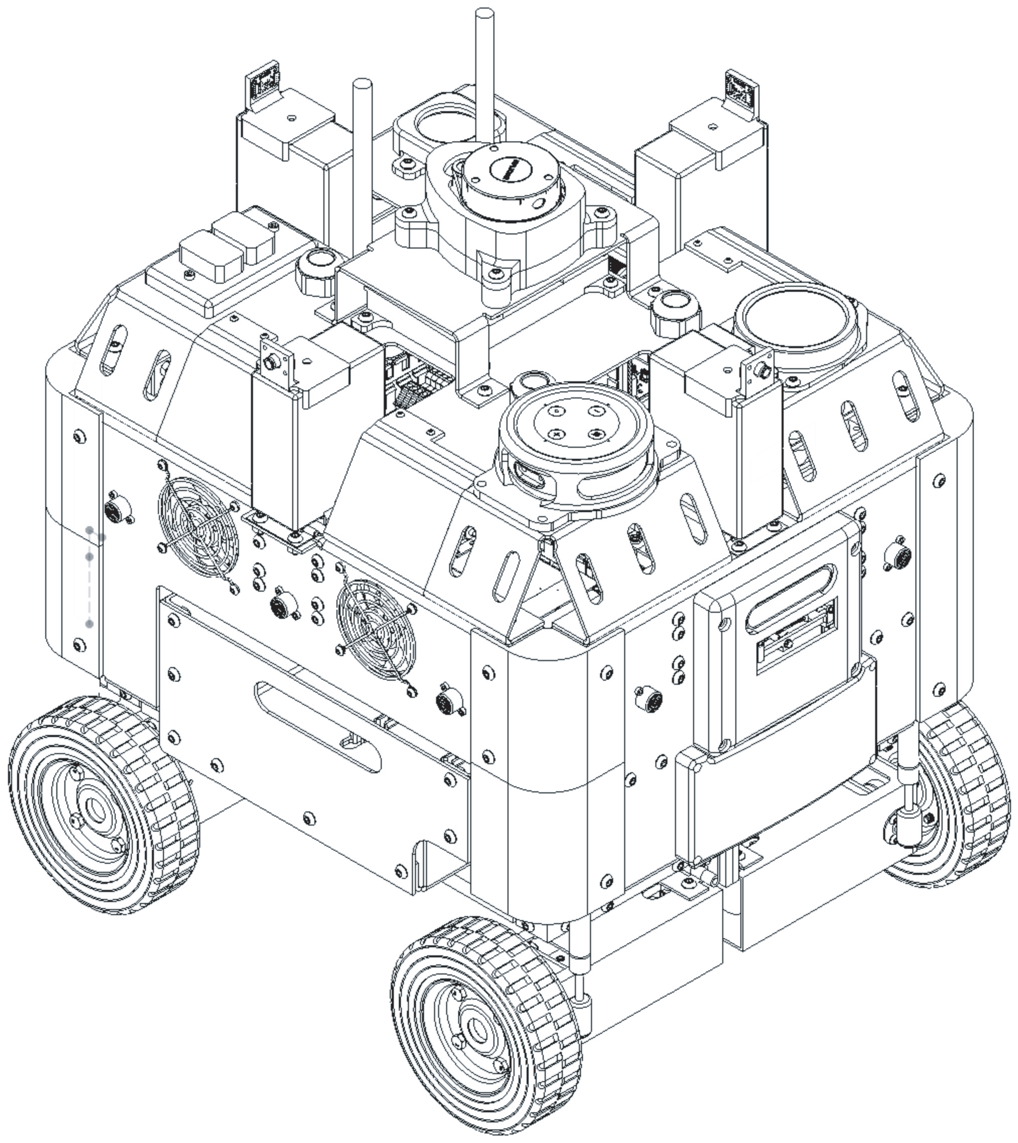
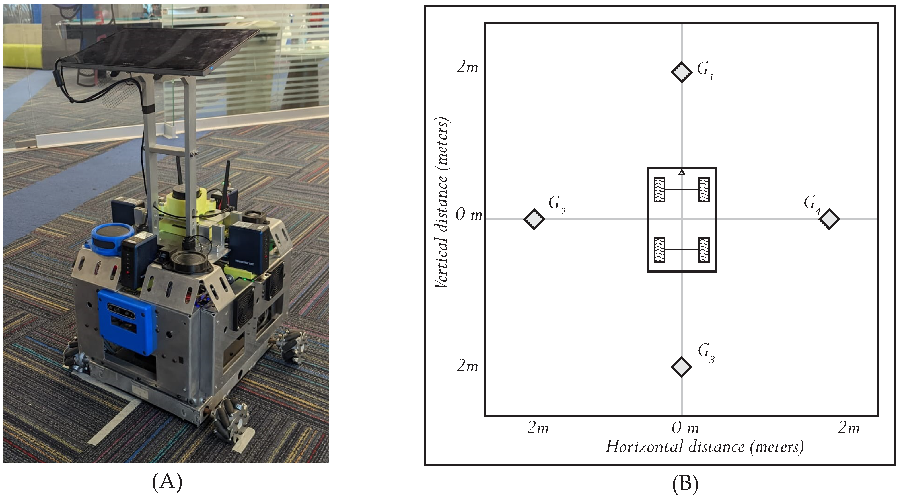
PiBot, a differential drive mobile robot detailed in
Figure 1, supports advanced navigation, smart surveillance, and research into control strategies and human–robot biometrics (temperature, distance, etc.). It demonstrates capabilities such as people counting, face mask validation, temperature measurement, and environmental monitoring in both closed and open scenarios. Notably, the MaskNet model previously tested on
PiBot achieved a peak accuracy of 70% for face mask detection in the static environment of the Tecnologico de Monterrey’s library, involving scenarios with pedestrian traffic [
32]. This work furthers the exploration of
PiBot’s utility in dynamic interaction scenarios, highlighting its potential for real-world surveillance and interaction applications.
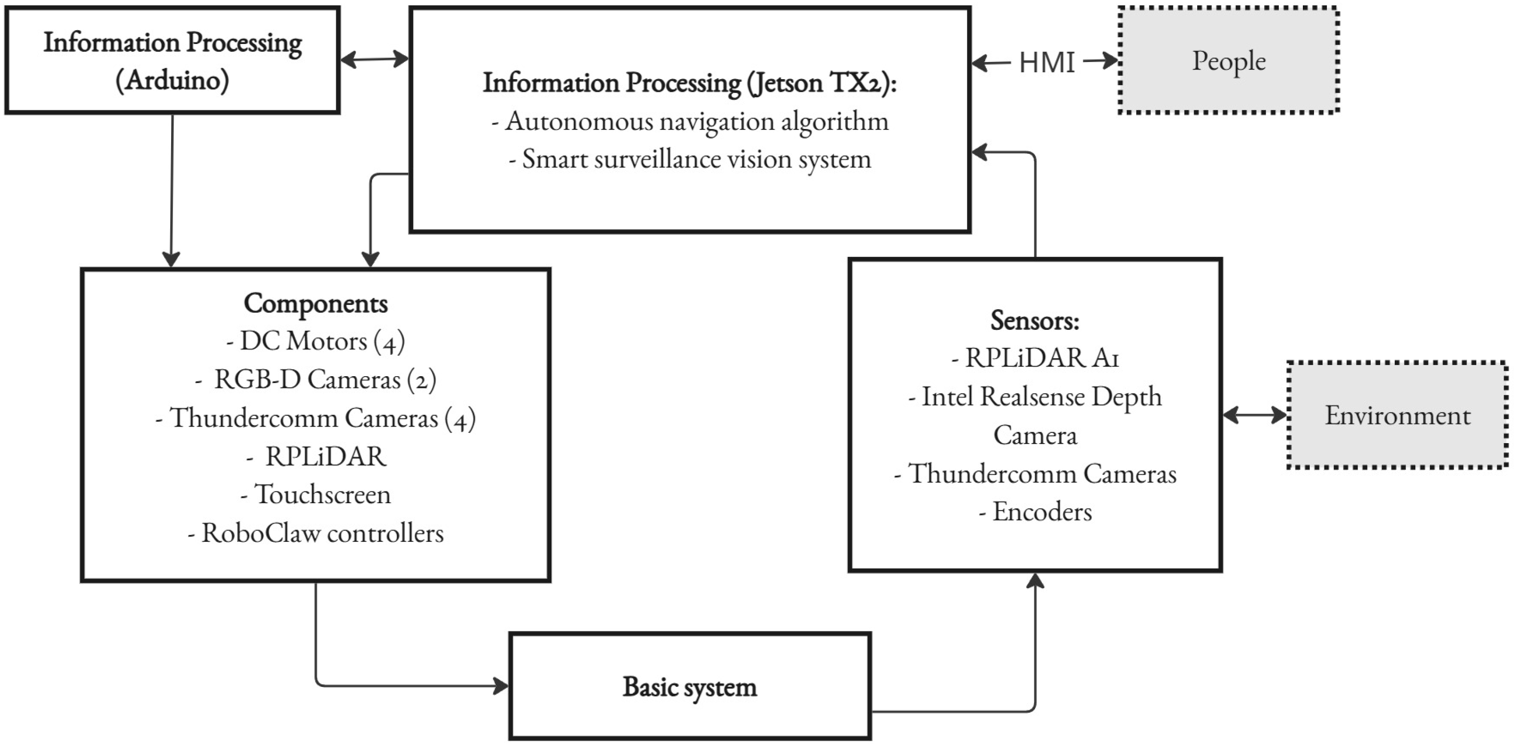
Figure 2 illustrates the mechatronic structure, showing the hierarchical organization and interactions among components. This architecture enables the robot to effectively process sensor data and execute both navigation and surveillance tasks.
In the following subsections, various aspects of the system are presented. The
Section 2.1 details the system’s physical properties, such as its dimensions, weight, and kinematic model. The
Section 2.2 discusses the hardware, connections, and components’ main tasks. Lastly, the
Section 2.3 examines the autonomous navigation, control, and vision system algorithms.
2.1. Mechanical Specifications
In this subsection, the mechanical specification of the proposed AMR is presented, focusing on its dimensions, system weight, spatial configuration in Cartesian coordinates, the robot’s kinematic model, odometry characterization, and the system’s actuators, providing a comprehensive understanding of the mechanical aspects of the system exhibited herein.
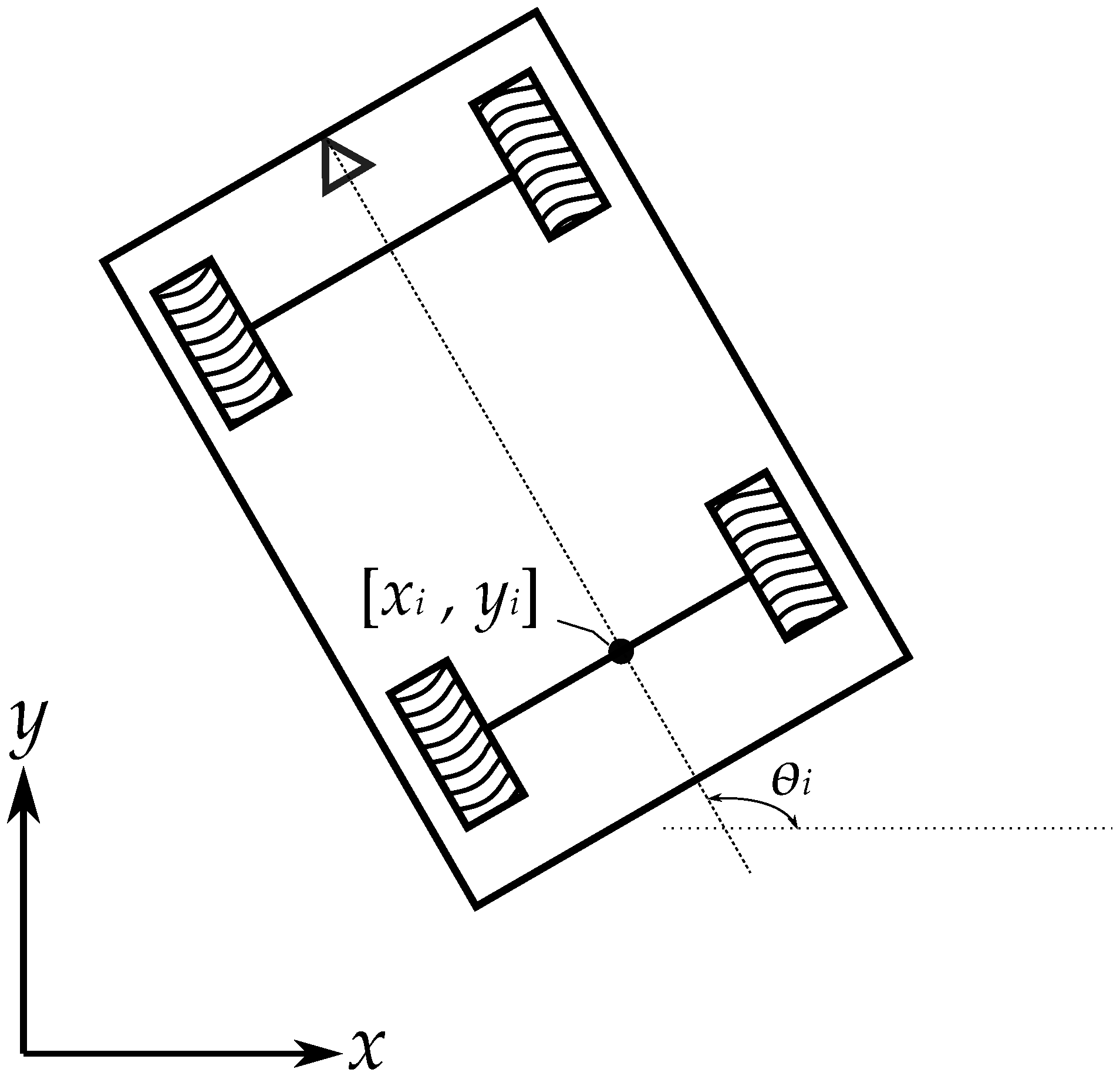
The robot has a rectangular aluminum chassis with length of 55 cm, width of 45 cm, a total height of 95 cm, and wheel diameter of 15 cm. The unloaded vehicle weighs approximately 25 kg. The configuration space of the differential drive mobile robot is that obtained by two Cartesian coordinates,
being defined over a real set of numbers and another coordinate,
, that is defined only over the numbers belonging to the angle of the unitary circle. This can be represented by
, which is a mathematical abstraction and a formalism of the physical states that the robot can achieve at any given time. A schematic of the robot’s plan is shown in
Figure 3, where the three variables of the robot’s position are shown.
2.1.1. Odometry Characterization
The transducers used in the odometry system are four Hall effect encoders, one located at each wheel that use an incremental tick for position estimation. Position estimation is carried out using the count of digital incremental encoders [
33]. Given the total number of encoder ticks per
N revolutions of the encoder, the distance traveled by the robot in the Cartesian space can be calculated using the following set of equations:
where
,
, and
are the distances traveled by the center point of the robot, the left wheel, and the right wheel, respectively, during a given time interval or movement,
L is the distance between the wheels of the robot on the same axis,
R is the radius of the wheels and,
and
are the increments in the count for the left and right encoders, respectively.
2.1.2. Kinematic Model
The model used for the differential drive mobile robot is presented in state-space form as follows:
where
is the linear velocity of the robot in the
x direction,
is the linear velocity in the
y direction, and
is the angular speed of the model referenced with the inertial frame. The model states are dependent on
and
, which are the angular speeds of the right and left wheels, respectively, and they can be computed as
where
v and
are the linear and angular velocities of the robot’s center point, respectively. These variables depend of the system’s current Cartesian pose. In this paper, the control strategy for the four-wheeled differential drive mobile robot capitalizes on the system’s intrinsic symmetry. Mobile robots with differential steering locomotion for classic wheel configurations can use the same equations as employed for two- and four-wheel drive platforms. This approach is effective due to the similar angular velocities exhibited by both wheels on each side of the robot [
34].
2.1.3. Actuators
The physical control actuator is a permanent magnet DC motor with a maximum rotational speed of 200 RPM and a nominal voltage of 12 V. The actuator’s speed is controlled internally with a motor control board, which enables speed control of the actuator as a linear system. The actuator model dynamics can be modeled as a first-order system, where
(RPMs of the permanent magnet DC motor) is the output of the system, and the input is the electric current signal delivered by the motor control board. The actuator control diagram is shown in
Figure 4.
2.2. Electrical and Electronic Specifications
In this subsection, the details of the hardware components used, and their interconnections, applications, interfaces, and tasks will be thoroughly explored, providing a comprehensive understanding of the electrical and electronic aspects of the system under investigation.
Hardware and Connections
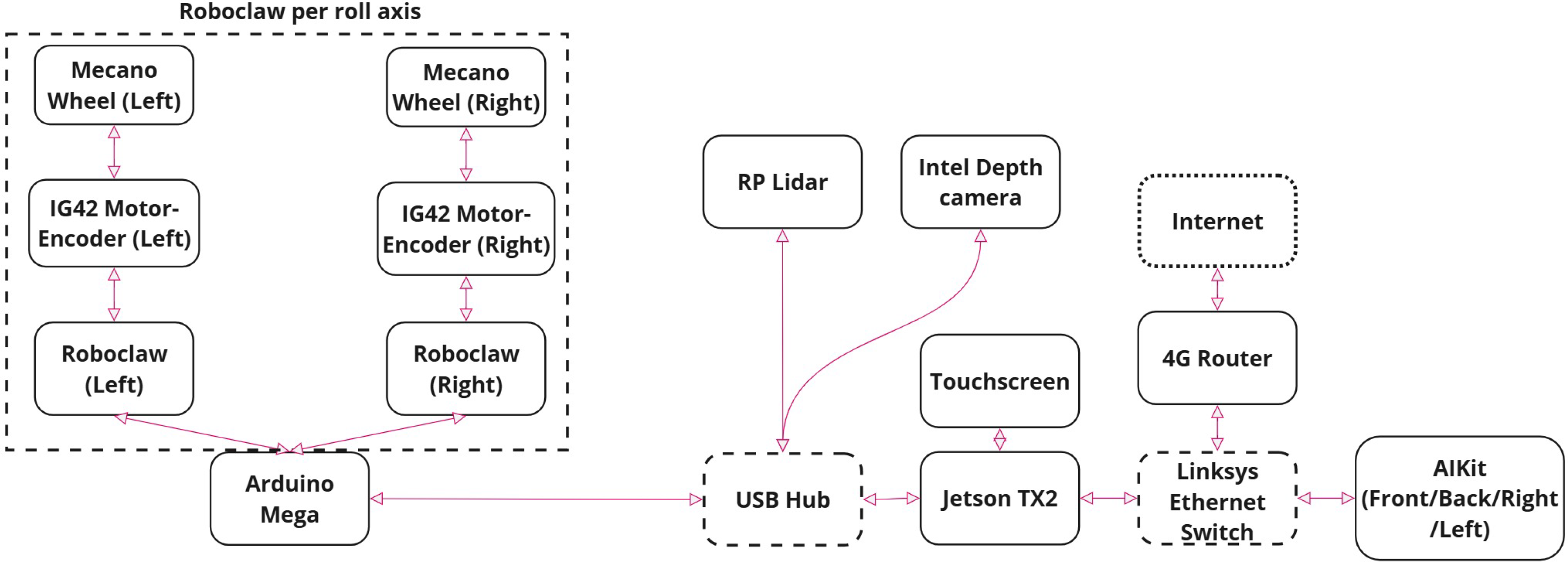
The system’s components consist of a Jetson TX2 (Nvidia) computer, which plays the role of the main computer running ROS, receives the messages from the different sensors and actuators, and performs computations on the acquired data for decision-making. This computer is connected to a USB Hub, which allows it to establish a serial connection with an Arduino Mega (Arduino), a LiDAR (Slamtec), and a 3D Camera (Intel). Additionally, the system includes a touch screen (ViewSonic) to interact with people, display messages, and function as a Human–Machine Interface (HMI).
The Arduino Mega executes a set of codes that process the information received from the Jetson TX2 to control the motors with a set of Roboclaw motor controllers (Basicmicro). The LiDAR is also connected to the USB Hub and sends data such as about the local environment and its estimated localization and orientation for the navigation algorithm (this process is explained in
Section 2.3). The 3D camera, which is also connected to the USB Hub, is capable of detecting people and the correct usage of face masks, and of sending messages to the Jetson TX2 to readjust the path plan. The component connection diagram is shown in
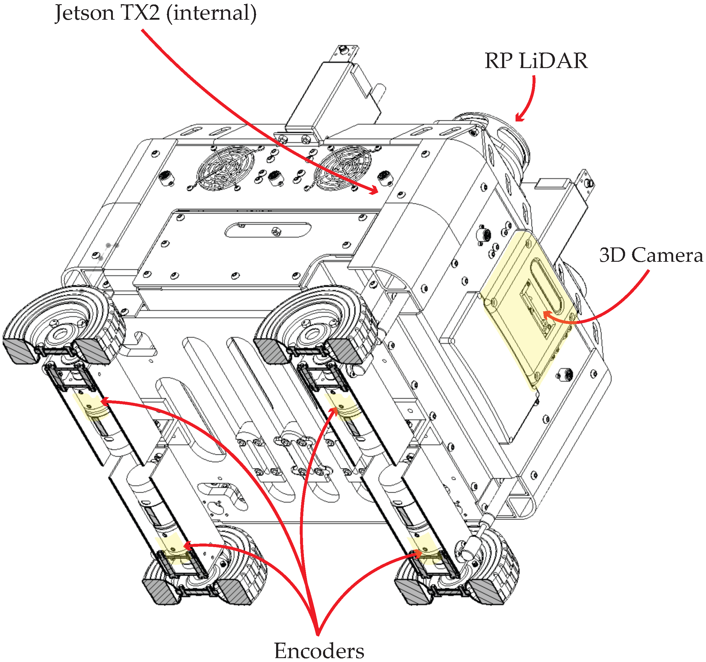
Figure 5. The main components required for the navigation system are the encoders on each motor, the LiDAR system, the 3D camera, and the Jetson TX2. These components and their location in the robot are shown in
Figure 6. The whole robot is powered by two LiPo batteries; the first is a LiPo 4s 14.8 V battery and is the main power source of the digital and control electronics; the second is a LiPo 6s 22.4 V battery and energizes the power electronics, as well as the motors.
The main hardware component of the vision system is the camera [
35]. In this robot, an Intel RealSense Depth Camera D435i was chosen, which has an IMU (Inertial Measurement Unit) capable of detecting depth under any situation when the camera moves. Due to this vision system working with artificial intelligence, a “digital brain” is required to carry out all the operations and processes necessary to perform the different tasks with very demanding calculations, offering maximum performance levels and relatively low power consumption [
36]. The robot makes use of an NVIDIA-branded Jetson TX2 for this purpose; which has robust hardware, hence its great performance capacity, with components integrated into the board including a Gigabit Ethernet port, WiFi and Bluetooth connectivity, 8 GB of RAM memory, and 32 GB in eMMC format. Other capabilities include working with two 4k video streams at 60 frames per second and simultaneously managing 6 cameras, and it also has a 64-bit processor and a 256-core Pascal GPU [
36].
2.3. Software Specifications
Lastly, in this subsection, the navigation algorithms, Navstack and Feedback controller, are described and compared, with Navstack being the primary choice for this robot. Additionally, the processing of the vision system will be detailed.
2.3.1. NavStack
The
Navigation Stack package is an open-source, cross-platform algorithm capable of running very simple robots up to really complex systems, offering the capability of autonomous navigation. The navigation process diagram is showcased in
Figure 7. The algorithm utilizes data from the odometry systems, built-in sensors, and a goal position, expressed as the vector
. This goal position is represented by a point position (
x,
y,
z) and a quaternion orientation (
x,
y,
z,
w). It is important to note that the
z value of the desired pose is always set to 0 because the navigation algorithm only considers the
x and
y components, disregarding the height (
z) value of maps. Consequently, the velocity commands generated by the algorithm are coherent and are dispatched to the mobile base of the system. This mobile base is incorporated into the
move_base package, executing actions such as moving towards and reaching a goal. The
move_base package employs both a local cost map (derived from the current LiDAR readings) and a global cost map (a previously created map of the environment), represented as an occupancy grid M, to achieve its navigation tasks [
37].
For a system to run the Navigation Stack package, a set of requirements must be met:
A planar laser must be mounted on the system for map building.
The robot shape must be circular or square, as the package was not designed for arbitrary shapes.
The system must be running ROS.
A transform tree that defines the relative location of each component.
The system must publish sensor data using ROS message types.
The algorithm works as follows: The desired goal is sent to the goal manager listener, which is a set of coordinates and an orientation. The system automatically generates a path using the stored map of the environment saved on the
global_costmap variable; then, Dijkstra’s algorithm calculates the shortest path available, using the robot’s current position as a global plan [
38]. Then, with the global plan to follow, the local planner generates velocity commands to send to a mobile base using the Dynamic Window Approach (DWA) [
39].
The local planner calculates the required speed
v and
of the system to reach the desired goal following a structured methodology. First, the system discretely samples the robot’s control space movement (
x,
y, and
), for each velocity, and performs a short-time simulation and predicts the outcome. These simulations are then evaluated with a score that considers aspects such as proximity to goal, proximity to global planner (based on map and not current sensor readings), and proximity to obstacles. The highest-scored trajectory is selected and implemented. This algorithm is then repeated. The velocity commands
v and
are re-adjusted using the local cost map generated continuously from the LiDAR measurements, and the system’s current position and orientation generated by the LiDAR with the Adaptive Monte Carlo localization (AMCL) algorithm [
40]. Once the velocity commands have been sent to the base controller, which requires data such as the wheelbase, track, and the wheels’ radius, it controls the wheels at the required speed according to the planned trajectory. The resulting change in position and orientation is estimated by the odometry system, to be considered by the AMCL algorithm and to readjust, if required, the trajectory following the DWA approach [
41].
2.3.2. Feedback Controller
The controller proposed is a variation of the control scheme implemented in [
42], as well as the one proposed in [
7,
43], where exponential stabilization is achieved via real State Feedback Control (SFC) using a geometric transformation of Cartesian coordinates to polar coordinates. To implement this control scheme, the kinematic model in Equation (
2) can be transformed into a point-in-plane model:
The position error is defined as the difference between the goal position
and the actual estimated position
x, the same operation applies for the desired
y coordinate. Let the output of the position error
and
, the model input for the speed is calculated as in Equation (
5) and for the angular speed as in Equation (
6), where
and
refer to the gains of the controller and
is the desired orientation angle in the control loop, computed as a function of the goal coordinates
and
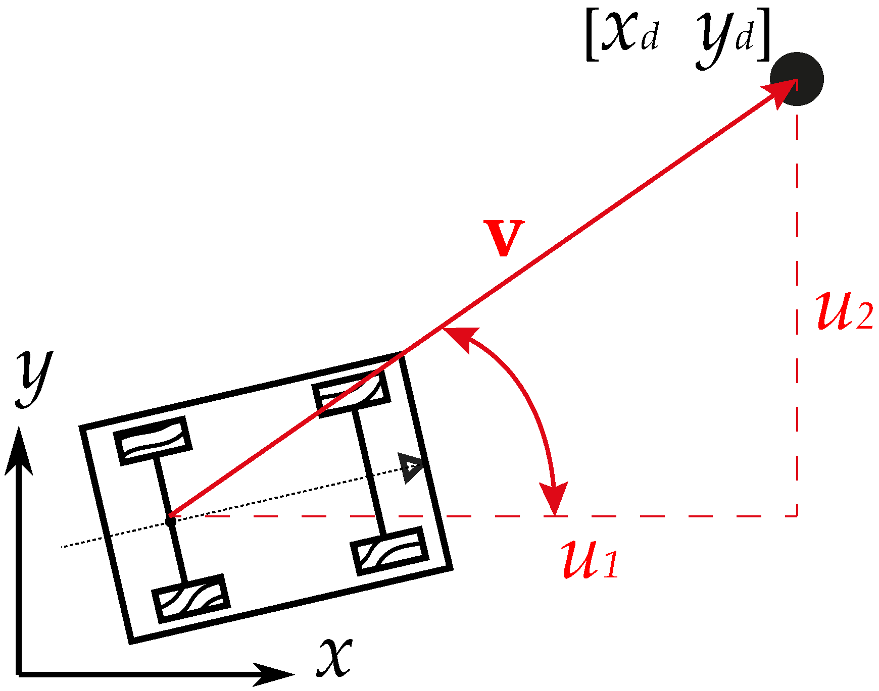
. A geometric interpretation of this control scheme can be seen in
Figure 8, the velocity vector
, pointing towards the goal is represented as a function of the positional error vector.
Parameter Choices and Model Scope: In our setup, the wheel radius R is 0.075 m, matching the physical wheels on PiBot and providing stable traction on high-friction indoor floors. The wheelbase L is set at 0.30 m, corresponding to the actual distance between the left and right wheels on the same axis. We assume negligible wheel slip under these lab-controlled conditions; more complex slip modeling would be required for uneven or low-friction terrains. Additionally, our sensor suite (encoders, LiDAR) is assumed to operate within nominal specifications, free of major signal dropouts or occlusions.
Standard Use of Cartesian-to-Polar Transformation: The conversion from Cartesian
coordinates to polar coordinates is a well-recognized practice in non-holonomic mobile robot control, helping to simplify the derivation of feedback control laws. We adopt it here for convenience and consistency with established techniques, rather than claiming a novel transformation. The overall implementation of this type of controller can be represented using the block diagram in
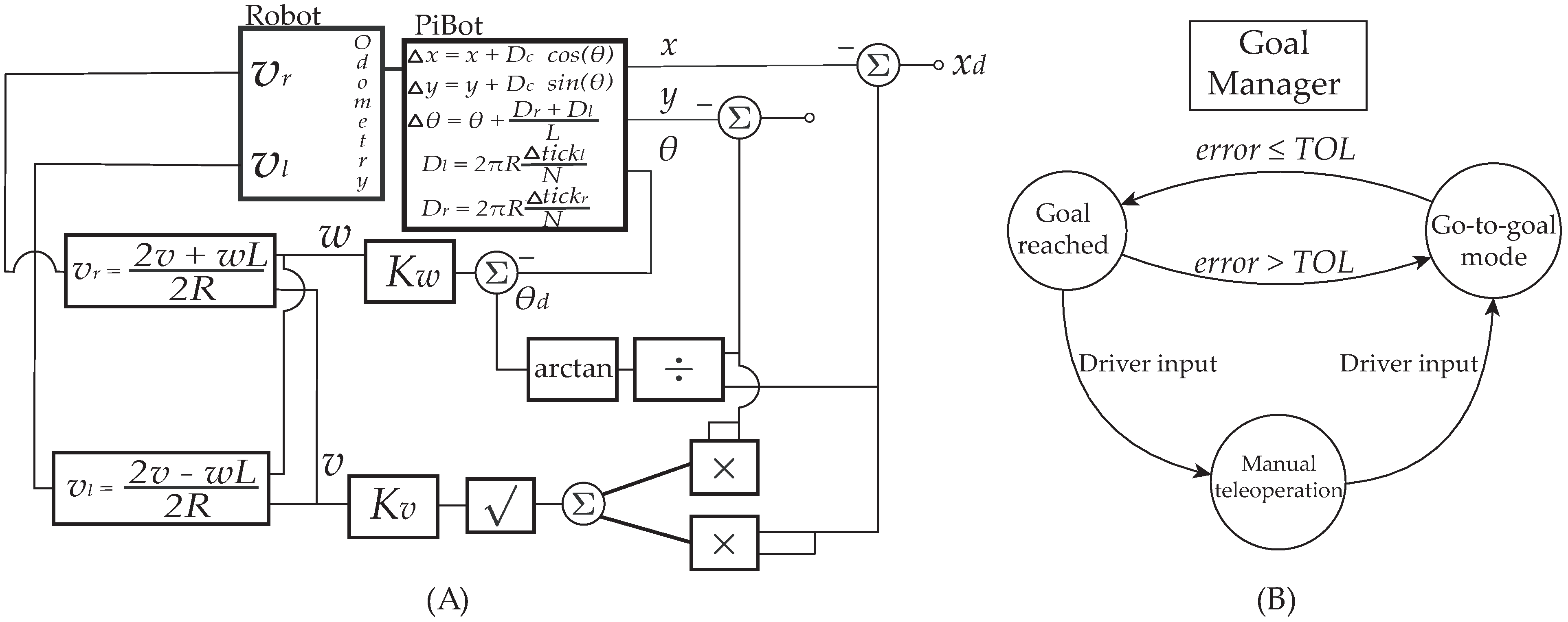
Figure 9A. The robot model to control can be seen as a block called
PiBot (name of the physical robot), from which the three states (position and orientation) can be obtained as a function of the odometry position estimation. On top of the go-to-goal low-level control, there coexists a finite state machine that regulates an arbitrary number of coordinates to reach the control system goal. The finite state machine can be seen in
Figure 9B, which can be seen as a basic
Go-to-goal scheme where the logic state of
Goal reached conditions the next dynamic state using the tolerance of the norm of the error
concerning the goal point, according to
.
2.3.3. Vision System
The vision system of
PiBot, detailed extensively in [
32], operates through a streamlined process involving person detection, image cropping, and face mask recognition. Utilizing YOLOv4 for efficient person detection through bounding boxes trained on the COCO database, the system employs the D435i camera’s sensors to assess social distancing between individuals. The synergy between these technologies underpins
PiBot’s advanced vision capabilities, which are explored in greater detail in the preceding vision work [
32].
4. Experimental Results
4.1. Experiment 1: Navigation Tests
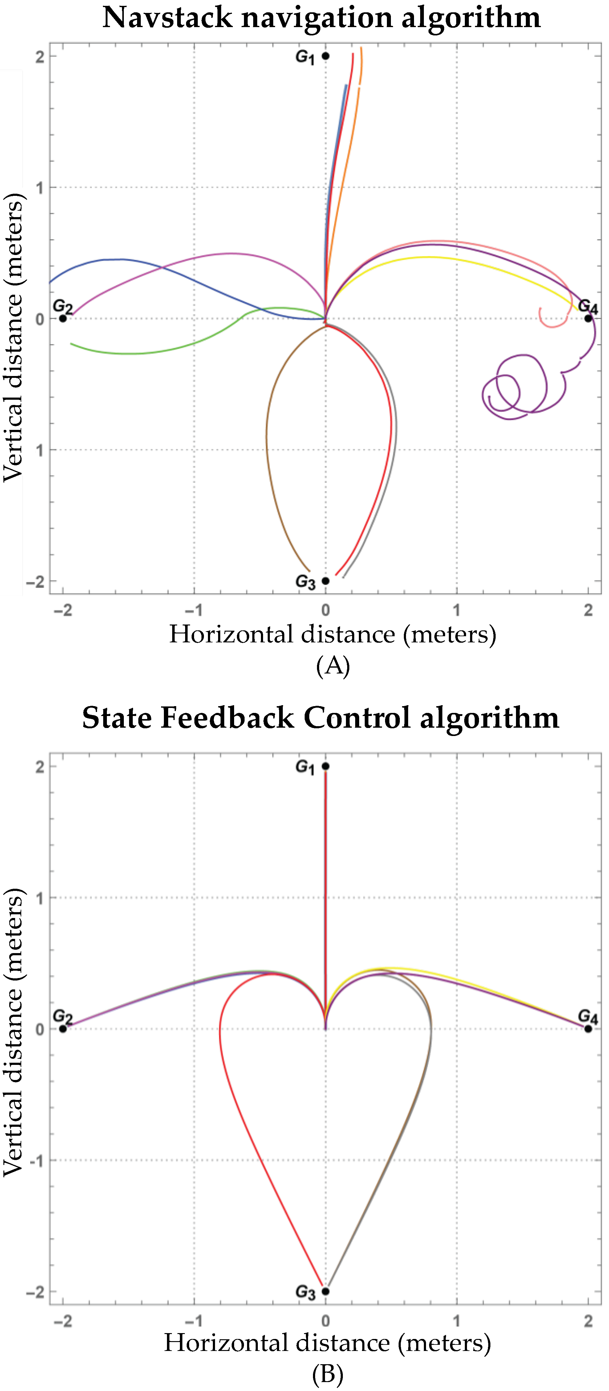
One outlier run toward
G4 produced a small loop near the goal (
Figure 12A, which inflated the overall Navstack mean to 0.26 ± 0.24 m. Removing that single run yielded a more representative error of 0.19 ± 0.10 m.
On the other hand, the trajectories during the 12 executions with the State Feedback Control algorithm are shown in
Figure 12B. This algorithm offered a better precision in reaching the desired position, following consistent and repeatable trajectories. In this case, the average error was 0.0412 ± 0.0014 m. Expressed as MSE, Navstack yielded
for the full set of 12 runs. These results, as mentioned above, were highly influenced by the last run dedicated to reaching
G4. The SFC controller produced
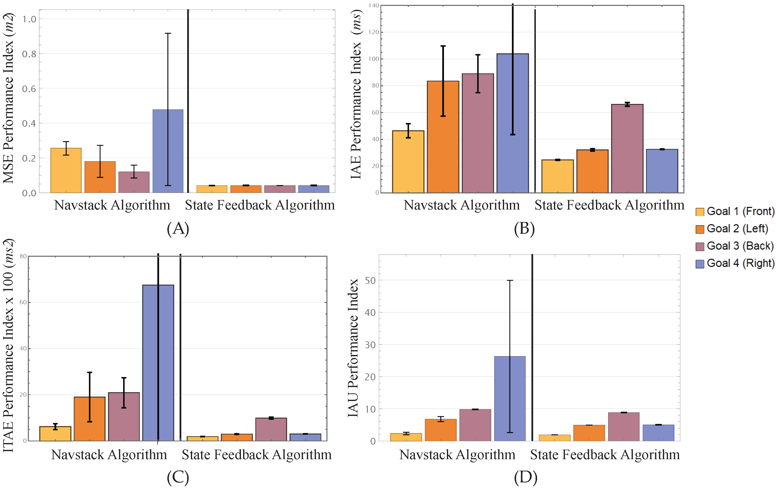
, two orders of magnitude lower. The top-left graph in
Figure 13 shows both algorithms’ average MSE and standard deviation per goal.
The average IAE with the Navstack algorithm was 80.70495 ± 36.30217 m
s throughout all runs. The State Feedback Control algorithm achieved an average IAE of 38.8357 ± 0.6929 m
s. The top-right graph in
Figure 13 shows the average IAE and standard deviation for both algorithms per goal. Regarding the ITAE, the Navstack algorithm accumulated an average of 2840.400532 ± 4610.664885 m·s
2 across all of its runs. Meanwhile, the SFC algorithm gathered an average of 445.4025 m ± 14.1986 m·s
2. This metric, just like the MSE metric, was highly affected by the error recorded in the last run reaching the
G4, shown as an erratic path forming loops when reaching the destination in
Figure 12A. The bottom-left graph in
Figure 13 displays the average ITAE and standard deviation per goal of both algorithms.
Finally, the average IAU index of the runs with the Navstack algorithm was 11.3139 ± 6.2265. In contrast, the SFC algorithm achieved an average index of 5.1986± 0.0657. The bottom-right graph in
Figure 13 shows the average IAU and standard deviation per goal for both algorithms. The SFC algorithm generated manipulation variables with lower magnitudes, i.e., a softer actuation. Statistical analysis revealed substantial practical differences between the algorithms across all metrics.
Table 2 lists the means, standard deviations, 95% confidence intervals, and bias-corrected Cohen’s
d for each goal. SFC outperformed Navstack by one to almost three orders of magnitude in MSE (large effects for G1–G3, moderate for G4) and lowered the overall manipulation effort (IAU) by about half on average. SFC satisfied the
accuracy criterion in all 12 runs, whereas Navstack did so in 7, confirming a superior point-to-point accuracy, trajectory repeatability, and actuation efficiency in this semi-structured indoor test.
4.2. Experiment 2: Vision Tests
Based on Experiment 2, the vision system performance was evaluated to examine the interaction between robots and humans under various conditions, specifically focusing on four metrics: accuracy, precision, recall, and
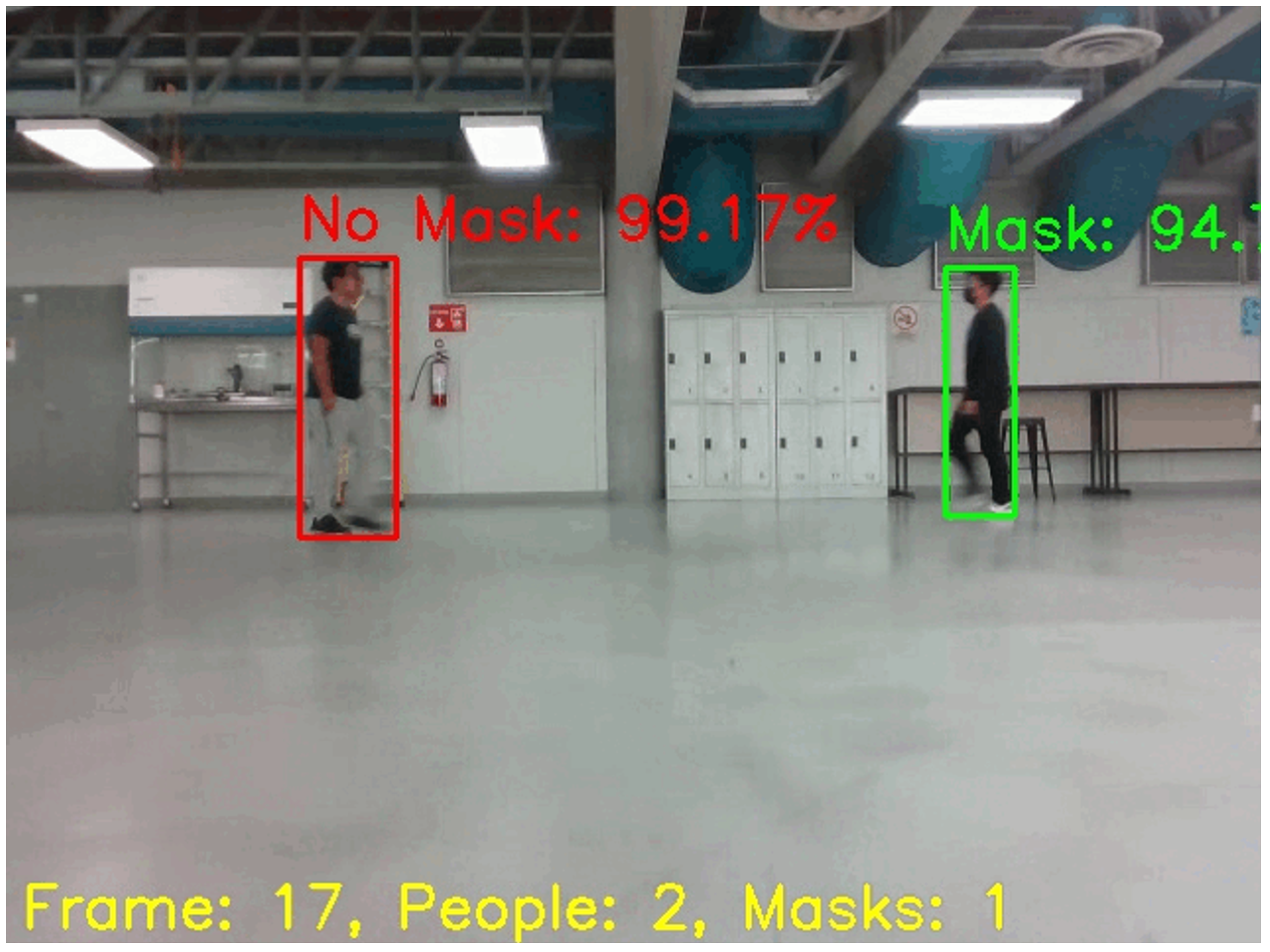
score. The analysis involved factorial regression models and ANOVA to determine the significant effects of robot speed (static or moving) and person speed (walking or running) factors. First, confusion matrices were produced for all configurations and the overall runs, presenting the true positives, true negatives, false positives, and false negative values counts for each condition.
Figure 14 displays an example frame from the vision system, depicting how people were detected and classified based on mask wearing, with confidence scores shown for both masked and unmasked individuals. These real-time classifications were compared against manual ground truth annotations to generate the confusion matrices.
Table 3 presents the confusion matrix for all possible configurations according to
Table 1, case A considered the static platform with walking people configuration, case B corresponded to the static robot and people running mode, case C was when the robot was moving and the people were walking, and finally case D was related to the robot moving and people running configuration.
Lastly,
Table 4 presents the confusion matrix considering all the runs together, obtaining the overall count for each
,
,
, and
.
The findings of this 2K Factorial Design were separated into the four metrics employed: the Accuracy, Precision, Recall, and score, presenting the findings for each metric when combined with all the terms and their interactions.
. With a p-value of , the “People Speed” factor proved significant with a 95% confidence level. By analyzing the main effect factorial plots, a broader difference between levels for the “People Speed” factor can be seen, with a difference of 8.21% between levels, with the “Walking level” around 73% accurate, while the “Running level” decreased to around 65%. Both ANOVA assumptions were met, with the Normality in the residuals test achieving a 0.723 p-value, while the Homoscedasticity test obtained a p-value of 0.879.
. With a 95% confidence level, no factor or term proved significant for the Precision metric. By analyzing the main effect factorial plots, a slight difference between levels in both factors is appreciable, but no significant effect was detected. Both ANOVA assumptions were met, with the Normality in residuals test achieving a 0.085 p-value, while the Homoscedasticity test obtained a p-value of 0.476.
. With a p-value of , the “People Speed” factor proved significant, with a 95% confidence level. By analyzing the main effect factorial plots, a broader difference between levels for the “People Speed” factor can be seen, with a difference of 25.13% between levels, with the “Walking level” around 70% Recall, while the “Running level” decreased to around 44%. Both ANOVA assumptions were met, with the Normality in the residual test achieving a 0.359 p-value, while the Homoscedasticity test obtained a p-value of 0.486.
Score. With a p-value of , the “People Speed” factor proved significant with a 95% confidence level. By analyzing the main effect factorial plots, a broader difference between levels can be seen for the “People Speed” factor, with a difference of 16.58% between levels, with the “Walking level” having around 72% F1 score, while the “Running level” decreased to around 55%. Both ANOVA assumptions were met, with the Normality in the residual test achieving a 0.087 p-value, while the Homoscedasticity test obtained a p-value of 0.868.
5. Discussion
Of the two navigation algorithms evaluated, State Feedback Control (SFC) consistently outperformed Navstack in positional accuracy. This finding impacts service robotics in environments demanding precise navigation and reliable vision. This performance gap (
Table 2) reveals a trade-off: Navstack avoids obstacles but sacrifices precision, while SFC excels in precision but ignores obstacles.
For each individual goal, SFC produced significantly lower mean position errors. On average, Navstack’s mean error was roughly 6.3 times larger than that of SFC. The consistently large effect sizes (most d > 0.8) across metrics quantify the substantial performance gap between approaches. While both algorithms achieved their goals, SFC demonstrated a remarkably consistent performance, evidenced by tight confidence intervals across all metrics. In contrast, Navstack showed high variability, particularly for G4, where the wide confidence intervals reflect an inconsistent performance.
Additionally, the SFC navigation algorithm generated more consistent trajectories since, in the same conditions, the trajectories followed using this algorithm were nearly identical, except for one run dedicated to reaching G3 located behind the home position, as shown in
Figure 12b). However, this exception was not critical, as both sides generated mirrored trajectories. On the other hand, the trajectories followed throughout the runs with the Navstack algorithm lacked consistency, as they tended to vary between different runs for the same desired goal, as shown in
Figure 12a). It should be noted that a critical factor for these navigation algorithms is the sensors from which they obtain the data used to estimate their position and orientation. The Navstack algorithm used both the motor encoders and the LiDAR global and local cost maps to estimate its position, while the SFC navigation algorithm relied only on the encoders. The encoders used in the system are highly accurate, and the tires exhibited little, if any, slippage, which would explain the excellent precision achieved with the SFC algorithm. Otherwise, oscillation of the system’s structure when moving or poor extrinsic calibration of the LiDAR system shifting the relative position and orientation could explain the significant errors obtained with the Navstack algorithm [
48]. Regarding the amount of information used to perform the navigation, it is safe to assume that the SFC could drive the system to the desired goal using less information than the Navstack local controller.
Unlike Navstack, the SFC controller cannot autonomously detect obstacles and re-plan to avoid them. This gives rise to the idea of creating a hybrid algorithm that runs on the SFC algorithm until it faces an obstacle; then, the Navstack algorithm would override the system to evade the obstacle, and then relinquish control to the SFC algorithm. The resulting fusion of algorithms would combine the best of both navigation algorithms by achieving the best possible trajectory in terms of precision and consistency, while being able to detect and evade obstacles. Additionally, the performance of the SFC algorithm can be explained by the appropriate selection of gains. On the other hand, the Navstack control was configured following the ROS Navigation Tuning Guide [
49] for indoor navigation and cornering behavior, with the DWA planner parameters optimized for our robot platform. However, not every parameter was optimized, which might explain the imperfect behavior observed. Further fine-tuning of additional parameters could improve performance.
The navigation experiment carried out was performed to display the capabilities for pure point-to-point motion, and one inherent limitation was that the obstacle avoidance techniques and metrics remained unevaluated. In that sense, a similar setup could be mirrored to replicate the experiment supposing that the navigation system detects one or more obstacles or enters obstacle-avoidance mode. In that case, the expected results would differ from the obstacle field and the method defined to avoid those obstacles.
The vision experiment extended the investigation into the performance of the vision system under various conditions of mobility, specifically comparing scenarios where the subject was either walking or running while the robot was either static or navigating forward, focusing on the impact of different speeds on the performance of the MaskNet model. The findings indicate a significant dependency of the vision system’s accuracy on the speed of the observed individuals. The mask detection accuracy and the rate of false negatives were notably better when subjects were walking as opposed to running. When comparing walking to running, there was a noticeable drop in accuracy, recall, and F1 score, with drops in performance of 8.21%, 25.13%, and 16.58%, respectively. The data suggest that the model’s ability to correctly identify and classify face masks decreased as the environment became more dynamic with people running.
Interestingly, while the robot’s speed (static vs. moving) did not significantly impact the overall performance, there was a slight, though not statistically significant, improvement in all metrics when the robot was in motion. This could be attributed to the varying angles and distances when capturing images while moving, aiding the vision system in more accurate detection, yet the improvement was minimal. The significant drop in accuracy during high-speed scenarios suggests the need for two key enhancements: first, implementing sequential analysis that considers consecutive frame inferences to reduce false positives, allowing the system to leverage temporal information from previous detections to validate current predictions; and second, expanding the training dataset to include more examples of subjects in motion at different speeds, which would help the model better recognize features under dynamic conditions.
6. Conclusions
PiBot showcases the integration of diverse sensors and components tailored for tasks such as environmental monitoring and autonomous navigation. The inclusion of AI kits within PiBot aids in processing vision models, reducing the computational load on its central Jetson TX2 computer. In its current form, PiBot demonstrates capabilities for sensor integration and data processing through mechanical and software integration. While the experimental validation focused on controlled indoor environments with optimal floor conditions (hospitals, universities, manufacturing warehouses, etc.), future research should expand testing to variable terrain conditions, for deployment in demanding outdoor or dynamic settings.
Experiments showed that PiBot achieved an average navigation error of 0.041 m with the SFC controller (versus 0.26 m for Navstack) and 71% mask-detection accuracy in static--walking scenarios, confirming the platform’s potential for service robot tasks. The State Feedback Control (SFC) algorithm showed a high precision and repeatability in navigation but lacks obstacle sensing and path adjusting when obstacles appear, making it only suited for obstacle-free environments. Further tuning of the navigation stack and calibrating the LiDAR sensor could enhance performance. To address SFC’s obstacle detection limitations, future work could use a hybrid approach: integrating SFC’s precision in open spaces, while allowing Navstack to override for obstacle evasion when required.
This potential arises from
PiBot’s hardware and software structure being similar to the systems presented in [
29], which have achieved accuracy rates greater than 90%. The experiment in dynamic environments revealed that the robot’s speed did not significantly impact the vision system’s effectiveness when navigating toward walking people. However, the speed of the individuals did influence the results, particularly affecting the detection of face masks and leading to an increased rate of false negatives, with a confidence level of 95%. These findings highlight the challenges the MaskNet model faces in environments with varying degrees of human activity. To address these limitations, future work will pursue several parallel improvements: first, exploring lightweight, optimized architectures that can maintain high accuracy, while working within the current hardware constraints; second, fine-tuning the existing model with a broader dataset that includes varied lighting conditions, movement speeds, and capture angles. The model is sensitive to people’s speed, something service robots in real-world dynamic scenarios constantly face.
