Model-Based AUV Path Planning Using Curriculum Learning and Deep Reinforcement Learning on a Simplified Electronic Navigation Chart

Abstract

Deep Reinforcement Learning (DRL)-based algorithms have demonstrated substantial effectiveness in tackling complex control problems for autonomous underwater vehicles (AUVs). This paper attempts to evaluate reinforcement learning (RL)-based methods for AUV trajectory planning by incorporating a model of a vehicle’s full motion. In this study, the agent (AUV) is assumed to have no prior knowledge of the environment in which it navigates. Instead, it only receives inputs from navigation sensors and a simulated sonar. Additionally, in the article, a reward function is proposed and described, along with its optimization process, to elicit the desired behaviors in the underwater vehicle. The models are trained and tested on simplified electronic navigation chart (ENC) maps, followed by a comparative analysis against five effective classical methods for trajectory planning. The proposed solution enables efficient, collision-free route planning for the autonomous underwater vehicle, taking its motion dynamics into account to reach the designated target successfully.

1. Introduction

Autonomous underwater vehicles (AUVs) continue to attract significant attention within the scientific community. They are employed in various fields, such as oceanography, the oil and gas industry, maritime rescue, military applications, underwater archeology, and photogrammetry. Research on the development of AUVs encompasses multiple areas, with a strong focus on enhancing vehicle autonomy. This includes the development of artificial intelligence and machine learning algorithms for improved decision-making capabilities [1,2] and increased precision in navigation and obstacle avoidance [3,4], as well as adaptive algorithms that can adjust to changing conditions [1].

Simultaneously, efforts are underway to advance underwater communications and data transmission. These include developing efficient underwater communication systems, such as acoustic and optical data transfer methods [5]; improving the connectivity between surface vessels and other underwater vehicles; and reducing latency while increasing the data throughput [6,7,8].

Maritime route-planning systems are generally assessed in terms of their total path length, adherence to safety contours (sometimes referred to as “safety isobaths”), and avoidance of restricted or prohibited zones, as well as ensuring path smoothness and sufficient separation from hazards. Vehicle motion models must accurately capture the AUV’s maneuvering capabilities so that the path-planning algorithm can account for the proper trajectory-following behavior [9,10,11]. External factors like ocean currents, tides, wave conditions, the accuracy of navigation systems, and the presence of obstacles affect path planning both prior to and during vessel operation. Consequently, an AUV should be capable of making autonomous decisions regarding the trajectory it follows.

Up to now, the research has predominantly centered on classical route-planning approaches, such as the A* algorithm and its numerous adaptations [12,13,14], Rapidly Exploring Random Trees (RRTs) [15,16], and Probabilistic Roadmaps (PRMs) [17,18]. Other trajectory planning strategies encompass fuzzy-inference-based methods [19,20], optimization techniques such as genetic algorithms [21,22] and particle swarm optimization [23]. Likewise, neural-network-based algorithms have been used to discover efficient paths, as discussed in [24,25].

Another branch of research focused on control and path planning for underwater vehicles is reinforcement learning (RL). It constitutes a field of machine learning that has been intensively developed in the last decade, both by technology companies [26,27,28] and by individual researchers. These methods involve studying and optimizing the interaction of an agent with its environment. During training, the algorithms collect experience from environmental data and the agent’s chosen actions. The objective is for the agent to perform a specific task by maximizing a reward function, which depends on the actions taken over the course of its interaction with the environment.

Reinforcement learning (RL) encompasses a broad range of algorithms that can be categorized in multiple ways. From the perspective of value functions or policy representation and updating, one can distinguish several groups: (1) tabular methods such as SARSA and Q-learning, typically relying on Q-value tables and temporal-difference updates for relatively low-dimensional state spaces [29,30]; (2) policy gradient approaches that directly optimize a parameterized policy; (3) actor–critic methods combining value-based and policy-based ideas; (4) hierarchical RL, which introduces higher-level structures or subgoals; and (5) evolutionary or genetic-based algorithms. Furthermore, Deep Reinforcement Learning (deep RL) extends these ideas by using deep neural networks to approximate value functions, policies, or even entire environment models, allowing for more effective handling of high-dimensional and complex tasks [31,32].

In [33], the SARSA algorithm was employed to build a hierarchical, two-level path-planning framework using a multi-SARSA strategy. This method extends the classical SARSA and reduces the training time while yielding shorter paths. Its operation integrates a topological map and artificial potential fields, effectively handling obstacle avoidance and converging more quickly compared to basic SARSA. This approach maintains two Q-tables: one for accelerating learning and another as part of the topological map. Meanwhile, Q-learning was applied in [34] to planning the route for a three-degree-of-freedom (3-DOF) marine vehicle. The RL algorithm was compared with standard path-planning methods such as A* and D*. Obstacles were not included in this study. Classic RL algorithms have also been used in more sophisticated scenarios, like flight route planning for UAVs [35].

Because route planning constitutes a high-dimensional problem, where the vehicle is operating in continuous space in both the control signals (actions) and the physical environment, classical algorithms are rarely effective for such use cases. They typically do not generalize well to broader settings. Consequently, using neural networks as function approximators within RL helps to address these limitations. Specifically, obstacles in the environment, numerous control signals, and the environment’s state vector do not hinder the application of these methods. Deep RL thus enables maritime route planning that can adapt in real time to changing ocean conditions. In [36], for example, the authors proposed a Deep Q-Learning approach to dynamic obstacle avoidance for autonomous surface vessels. A key novelty is its real-time obstacle avoidance capability, which enhances the computational efficiency, thereby allowing vessels to plan routes in changing conditions. The proposed algorithm integrates deep RL techniques with simulations of real-world conditions, representing a more advanced level of adaptive navigation than was previously available for surface vessels.

In [37], an adaptive path-planning method for an underwater vehicle was proposed using the Twin-Delayed Deep Deterministic Policy Gradient (TD3) algorithm. The algorithm successfully controlled a simulated Unmanned Surface Vehicle (USV) modeled in 6-DOFs (the Remus model), taking into account simulated ocean currents and dynamically introduced obstacles. Obstacle avoidance was achieved based on navigational sensor data measuring both the range and bearing to navigational hazards.

A different approach was presented in [38], where Proximal Policy Optimization (PPO) was employed for route planning and collision avoidance in autonomous surface vessels. A 3-DOF motion model was used, reflecting specific dynamic properties such as speed, drift, and rotation. The system relies on the collision risks proposed by the authors and complies with the COLREG rules for avoiding collisions at sea.

In [39], the authors present a method for the optimal trajectory tracking control over AUVs using DRL. They employ the Deep Deterministic Policy Gradient (DDPG) algorithm to train neural networks that generate precise control signals for the AUV. Simulations demonstrate that this approach outperforms traditional PID controllers in terms of its trajectory tracking accuracy, especially in complex and uncertain marine environments.

An interesting approach is presented in [40]. This paper addresses the problem of position tracking and trajectory control for AUVs using a rapidly deployable DRL method. The authors propose an approach that allows the DRL agent to be trained quickly and effectively deployed in real-world scenarios. The method achieves both position tracking and trajectory control, demonstrating excellent generalization capabilities.

In addition, in [41], the authors focused on path tracking for underactuated Unmanned Underwater Vehicles (UUVs) under conditions of intermittent communication. The authors developed a reinforcement-learning-based method that enabled the UUV to effectively follow a planned path despite communication constraints. Simulations show that the proposed approach ensures stable and accurate path tracking, even in the presence of model uncertainties and environmental disturbances.

The use of deep RL for docking tasks was demonstrated in [42]. In this work, the authors employed the DDPG and Deep Q-Network (DQN) algorithms to dock with a stationary platform. The comparative simulations included classical control methods such as Proportional–Integral–Derivative (PID) controllers and parametric optimal control. The results indicated that the DQN-based control provided faster docking while requiring less thrust power and a lower energy consumption. More recently, in [43], the authors focused on the docking problem in a realistic ocean environment, taking into account factors such as currents and noisy sensor data. In this work, the authors provide an Extended Kalman Filter (EKF) to fuse the raw noisy data. This enables the agent to effectively learn stable policies in the noisy environment, outperforming traditional control and policy methods that were obtained in noiseless environments. Furthermore, in [44], the authors focus on three-dimensional docking control for AUVs using DRL. They develop a method that enables AUVs to dock precisely in 3D space. Simulations demonstrate that the proposed approach features a faster learning process, greater robustness to disturbances, and effective control capabilities for achieving 3D docking.

Resource scheduling based on DRL has been explored in UAV-assisted emergency communication systems [45], focusing on optimizing limited bandwidth and power in critical circumstances. In a similar vein, 3D UAV trajectory planning for energy-efficient and fair communication was studied in [46], showcasing how DRL can handle multi-objective constraints in high-dimensional action spaces. Moreover, multi-agent cooperation in aerial computing systems [47] demonstrates the capability of RL to coordinate multiple agents under shared resource limitations.

This study presents a deep RL approach to determining and executing the trajectory for an AUV in a simplified (binary) ENC map environment. A 6-DOF model of the underwater vehicle is designed to achieve the shortest possible arrival path to the destination point. To enable a comparison, off-policy RL algorithms are utilized, including Soft Actor–Critic (SAC) with and without Hindsight Experience Replay (HER), Twin Delayed DDPG (TD3) with and without HER, and Truncated Quantile Critics (TQCs) with and without HER. The performance of these methods is benchmarked against five widely recognized classical algorithms known for high-efficiency collision-free path planning.

Table 1. Comparative overview of RL-based path planning methods for underwater and surface vehicles (2015–2025).

Title (Year)	Map Type	RL Algorithm	Motion Model	Environment	Platform	Key Contribution
AUV Obstacle Avoidance via Deep RL (Yuan et al., 2021) [48]	Active sonar (mapless)	Double DQN (LSTM)	3-DOF dyn.	Simulation	AUV	End-to-end obstacle avoidance using sonar inputs. Demonstrates collision-free navigation in unknown areas underwater.
Path Planning under Ocean Currents with DDQN (Chu et al., 2023) [49]	2D grid	Double DQN (CNN)	Dynamic (w/current)	Simulation	AUV	Incorporates current disturbances into the CNN-based planner. Outperforms A* and RRT in strong current fields.
SAC-Based Game Training for AUV Maneuvers (Wang et al., 2022) [50]	Random obstacles	SAC (game-theoretic)	Dynamic	Simulation	AUV	Adversarial approach with policy adaption to the environment (obstacles). Improves robustness under high uncertainty.
Adaptive Deep RL for 3D Navigation (Politi et al., 2024) [51]	Vision-based, mapless	PPO	6-DOF dyn.	Simulation	AUV	End-to-end 3D navigation using visual inputs. Stably achieves goals in complex underwater spaces.
Noisy Dueling Double DQN for AUV (Liao et al., 2024) [52]	2D grid + current data	ND3QN	Kinematic (drift)	Simulation	AUV	Uses dueling Q-nets with parametric noise for better exploration and stable training. Handles variable currents.
Improved PPO for USV Obstacle Avoidance (Sun et al., 2023) [53]	Radar-based local map	PPO (CNN)	Dynamic	Simulation	USV	Modified PPO with priority replay and a CNN architecture for the radar input. Converges faster and avoids collisions effectively.
Offline RL for USV Trajectory Tracking (Zhou et al., 2024) [54]	N/A (route known)	SAC (ensemble)	Dynamic	Sim + real	USV (full-scale)	Offline-trained controller validated in simulations and sea trials. Robust to waves and currents.
DDPG-Based Global Path Planning for USVs (Zhao et al., 2023) [55]	2D grid (static obs.)	DDPG	Kinematic	Simulation	USV	A global planner surpassing A* and heuristics in its path length, safety, and computation time.
Safe Lyapunov-DDPG for Target Interception (Du et al., 2022) [56]	No map (moving target)	SLDDPG	Dynamic	Simulation	USV	Integrates Lyapunov constraints for safe interception. Ensures bounded errors and avoids collisions.
Multi-AUV Cooperative Hunting with MAPPO (Wang et al., 2025) [57]	No explicit map	MAPPO	Dynamic	Simulation	Multi-AUV	Knowledge-guided policy from potential fields. Coordinates multiple AUVs for target pursuit under currents.
Our manuscript (2025)	Simplified ENC (binary)	SAC, TD3, TQC	6-DOF dynamic (full motion model)	Simulation (real port map)	AUV	Proposes a curriculum-trained deep RL approach on a real-world ENC map, integrating a full 6-DOF AUV motion model. Demonstrates smooth, high-speed collision-free trajectories. Outperforms classical methods (A*, PSO, GA) in its success rate and mission time across multiple scenarios.

provides an overview of selected works (from 2015 to 2025) on the application of reinforcement learning methods to path planning for surface (USV) and underwater (AUV) vehicles. This summary covers various map types (e.g., grid-based, sonar data, vision, and simplified maps), different degrees of complexity of the motion models (3–6 DOFs), and diverse RL algorithms (e.g., DDPG, PPO, SAC, and DQN). Additionally, it highlights key outcomes and findings, such as effectiveness in obstacle avoidance, handling of ocean currents, and adaptation to uncertain environments.

Compared to these earlier studies, this article introduces the following innovative elements:

• The use of a full 6-DOF AUV motion model for training and validation (in most prior works, the model is typically simplified to 3–4 DOFs);
• Experiments based on real ENC map data (converted into a simple binary grid derived from electronic navigational charts of the port of Gdynia), significantly bridging the gap between the training conditions and real-world applications;
• A comparison of three advanced off-policy algorithms (SAC, TD3, and TQC) with classical methods (A*, APF, GA, PSO, and RRT*), while also incorporating Hindsight Experience Replay (HER) and curriculum learning;
• An extensive multiparametric analysis (accuracy, distance, speed, and mission time) confirming that the TQC-based approach offers both high success rates (near 99%) and short execution times.

The remainder of this article is organized as follows: Section 2 describes the mathematical model of the AUV used both to train the RL-based algorithms and verify the feasibility of the trajectories obtained using the classical methods. This section also outlines the RL-based and classical methods, along with the procedure for path smoothing and trajectory generation. Section 3 details the agent’s training environment, including the observation and action spaces, as well as the reward function. Section 4 presents the optimized hyperparameters for the RL algorithms and discusses their training process. In Section 5, the simulation results for a path-planning task in the nonlinear AUV model are analyzed. Section 6 provides a discussion of the key aspects of trajectory planning based on the results obtained. Finally, Section 7 concludes this paper with a summary of its main findings and future work.

2. Materials and Methods

Global path-planning methods for AUVs can generally be classified into two categories: those that incorporate a dynamic model of the vehicle and those based solely on kinematic constraints. In this section, the nonlinear AUV model utilized in this study is presented, along with the RL methods that directly leverage this model. Additionally, a brief overview of the classical path-planning algorithms used is provided, followed by a discussion on how the generated paths are smoothed and converted into feasible trajectories while considering the motion constraints of the AUV.

2.1. The Nonlinear Mathematical Model of the AUV’s Dynamics

To achieve a highly accurate representation of the AUV’s motion and to provide realistic conditions for the control algorithms, a nonlinear mathematical model was used to describe the motion of the autonomous underwater vehicle (AUV) with both kinematic and dynamic constraints. The following assumptions are made for this model [10]:

• The AUV is treated as a rigid body with three planes of symmetry moving in six degrees of freedom and has a longitudinal plane of symmetry, which is also the plane of symmetry of the mass distribution.
• The vehicle moves in viscous fluid at a low speed and has a torpedo-like shape.
• The origin of the stationary coordinate system overlaps with the center of gravity.
• The mass distribution, moments of inertia, and deviant moments of a vehicle operating in a movable coordinate system are constant.
• The parameters responsible for the AUV’s dynamics are determined for a torpedo-shaped vehicle with a 45 kg mass and a 0.3 m diameter. These parameters could easily be adapted to other AUVs. 
• The PID controller parameters are tuned using a genetic algorithm [58].
• The model does not include limitations on the driving system because it is not focused on a specific driving system.

The model is based on equations for motion in six DOFs, which, using the SNAME notation [59], take the following matrix–vector form:

$$\begin{array}{c}\hfill M\left(\dot{v}\right)+D\left(v\right)v+g\left(\eta \right)=\tau \end{array}$$

(1)

where

• v—a vector of the linear and angular velocities in the movable system, expressed as

  $$v=[u,v,w,p,q,r]$$

  (2)
• $\eta$—a vector of the coordinates for the vehicle’s position and its Euler angles in an immovable system, expressed as

  $$\eta =[x,y,z,\varphi ,\theta ,\psi ]$$

  (3)
• M—a matrix of inertia, which is the sum of the matrices of the rigid body $M_{RB}$ and the added masses $M_A$, expressed, respectively, as

  $$M_{RB}=\left[\begin{array}{cccccc}m& 0& 0& 0& 0& 0\\ 0& m& 0& 0& 0& 0\\ 0& 0& m& 0& 0& 0\\ 0& 0& 0& I_x& 0& 0\\ 0& 0& 0& 0& I_y& 0\\ 0& 0& 0& 0& 0& I_x\end{array}\right]$$

  (4)

  $$M_A=-\left[\begin{array}{cccccc}{X}_{\dot{u}}& 0& 0& 0& 0& 0\\ 0& Y_{\dot{v}}& 0& 0& 0& 0\\ 0& 0& Z_{\dot{w}}& 0& 0& 0\\ 0& 0& 0& K_{\dot{p}}& 0& 0\\ 0& 0& 0& 0& M_{\dot{q}}& 0\\ 0& 0& 0& 0& 0& N_{\dot{r}}\end{array}\right]$$

  (5)
• $D\left(v\right)$—a hydrodynamic damping matrix, expressed as

  $$D\left(\nu \right)=\left[\begin{array}{c}\begin{array}{cccccc}{X}_u+(X_{\left|u\right|}\left|u\right|)& 0& 0& 0& 0& 0\\ 0& Y_v+(Y_{\left|v\right|}\left|v\right|)& 0& 0& 0& 0\\ 0& 0& Z_w+(Z_{\left|w\right|}\left|w\right|)& 0& 0& 0\\ 0& 0& 0& K_p+(K_{\left|p\right|}\left|p\right|)& 0& 0\\ 0& 0& 0& 0& M_q+(M_{\left|q\right|}\left|q\right|)& 0\\ 0& 0& 0& 0& 0& N_r+(N_{\left|r\right|}\left|r\right|)\end{array}\end{array}\right]$$

  (6)

  where
  • $X_u,Y_v,Z_w$—the first-order damping coefficients for the forces in the $X,Y,Z$ directions;
  • $K_p,M_q,N_r$—the first-order damping coefficients for the moments in the $K,M,N$ directions;
  • $X_{\left|u\right|},Y_{\left|v\right|},Z_{\left|w\right|}$—the second-order damping coefficients for the forces in the $X,Y,Z$ directions;
  • $K_{\left|p\right|},M_{\left|q\right|},N_{\left|r\right|}$—the second-order damping coefficients for the moments in the $K,M,N$ directions.
• $g\left(\eta \right)$ is a vector of the restoring forces and the moments of forces of gravity and buoyancy, expressed as

  $$g\left(\eta \right)=\left[\begin{array}{c}(P-B)·sin\theta \\ (P-B)·cos\theta ·sin\varphi \\ -(P-B)·cos\theta ·cos\varphi \\ (z_G·P+y_B·B)·cos\theta ·cos\varphi -(y_G·P+z_B·B)·cos\theta ·sin\varphi \\ -(z_G·P+z_B·B)·sin\theta ·cos\varphi +(x_G·P+x_B·B)·cos\theta ·cos\varphi \\ 0\end{array}\right]$$

  (7)

  where
  • P—the weight of the body;
  • B—the force of buoyancy;
  • $x_G,y_G,z_G$—coordinates of the center of gravity;
  • $x_B,y_B,z_B$—coordinates of the center of buoyancy;
  • $\theta$—the pitch angle;
  • $\varphi$—the roll angle.
• $\tau$—a vector of the control signals (the sum of the vector of the forces and moments of the force generated by the propulsion system ${\tau }_p$ and by environmental disturbances ${\tau }_d$).

  $$\tau =\left[\begin{array}{c}X,Y,Z,K,M,N\end{array}\right]$$

  (8)

The following simplifications were considered in the AUV simulation model:

• The mass deviation moments corresponding to the respective axes of the movable coordinate system were omitted due to their insignificance to the simulation.
• The $C\left(v\right)$ matrix was omitted from the mathematical model due to its negligible numerical influence under the assumed operating conditions. The propulsion system imposes strict dynamic limits, with the maximum thrust along the surge axis constrained to 25 N and the maximum yaw moment limited to 2 Nm. As a result, the AUV operates at relatively low forward velocities, up to approximately 2 m/s. This limited yaw moment further restricts the vehicle’s ability to perform aggressive turning maneuvers. These constraints ensure that the inertial effects represented by the $C\left(v\right)$ matrix, such as the Coriolis and centripetal forces, remain minimal and do not significantly affect the simulated vehicle dynamics [60].
• Hydrodynamic damping components greater than 2nd-order are omitted (the vehicle is operating at a low speed, the motion is not connected, and it has three planes of symmetry).

Two reference frames are used to analyze the motion of the AUV. The first is a body-fixed moving reference frame, whose origin corresponds to the vehicle’s center of gravity. The second is an inertial reference frame, which is fixed to the Earth. The position of the AUV in space is defined relative to the inertial reference frame, whereas the linear and angular velocities are described with respect to the body-fixed moving reference frame.

The transformation of the vehicle’s linear velocities from the body-fixed frame to the rate of change in its position coordinates in the inertial frame can be performed using the transformation matrix, as expressed in

$${\dot{\eta }}_1=J_1\left({\eta }_2\right)$$

(9)

where

$J_1\left({\eta }_2\right)$—a transformation matrix dependent on the Euler angles, defined as

$$J_1\left({\eta }_2\right)=\left[\begin{array}{ccc}cos\psi cos\varphi & -sin\psi cos\varphi +cos\psi sin\theta sin\varphi & sin\psi sin\varphi +cos\psi sin\theta cos\varphi \\ sin\psi cos\theta & cos\psi cos\varphi +sin\psi sin\theta sin\varphi & -cos\psi sin\varphi +sin\psi sin\theta cos\varphi \\ -sin\theta & cos\theta sin\varphi & cos\theta cos\varphi \end{array}\right]$$

(10)

The inverse transformation is defined as

$${\nu }_1=J_1^{-1}\left({\eta }_2\right){\dot{\eta }}_1$$

(11)

It should be noted that the model does not account for external forces such as ocean currents or inaccuracies in the position estimation.

The model utilizes PID controllers to regulate key motion parameters, including the longitudinal speed (u), depth (z), trim angle ($\theta$), and course angle ($\psi$). The PID controllers compute the required forces and moments $\mathit{\tau }$ based on the difference between the setpoint value $p_s$ and the current state of the vehicle. PID controllers were employed in this context to ensure uniformity across all tested planning methods and to decouple the evaluation of these methods from the complexities of motor-level control. This approach was intended to ensure that both classical and DRL-based planning strategies could be evaluated fairly, without being biased by the characteristics of the low-level controller.

The modeled torpedo-like AUV can execute maneuvers to avoid obstacles by adjusting its depth, course, or forward speed. Since horizontal-plane maneuvers are most commonly used, this paper assumes that AUV control will be performed through course and speed adjustments.

Employing a 6-DOF model of the AUV allows for an accurate representation of vehicle behavior in an underwater environment. In reinforcement learning, the agent learns from interactions with its environment; hence, using a realistic motion model ensures that the agent’s experiences closely resemble those in the real world. With a comprehensive dynamics model, an RL agent can learn complex maneuvers such as navigating in three-dimensional space, avoiding obstacles in a dynamic setting, and adapting to changing conditions—like varying ocean currents or different operating depths (not accounted for in this paper). Moreover, an AUV model enables the RL agent to optimize control strategies aiming to both minimize the energy consumption and enhance safety by learning to avoid collisions and stabilize the vehicle in challenging circumstances. The more realistic the simulation model, the greater the likelihood that the trained policies will transfer effectively to real AUV operations, thus reducing the time and cost of real-world testing.

2.2. The Reinforcement Learning Background

Reinforcement learning encompasses methods that enable an agent to develop a policy $\pi$, guiding its future behavior through interactions with the environment. If a particular action a leads to a better performance (i.e., higher accumulated rewards), the algorithm reinforces the agent to execute this action more frequently. RL can be viewed as unsupervised learning: the agent gathers scalar feedback (rewards) based on its interactions with the environment. The agent’s performance is measured by analyzing these collected rewards, which in turn allow it to optimize its actions to maximize them.

At each time step t, the agent, in state s, performs an action a. As a result, it transitions to a new state $s^{\prime }$ and receives a reward r. Note that receiving a reward r at every transition is not mandatory in all environments; it is specific to so-called dense reward settings, as studied in this work. Given that the subsequent state $s^{\prime }$ depends only on the current state s and action a, rather than on any prior states or actions, the Markov Decision Process (MDP) framework is used to describe the system dynamics. This framework helps the agent learn the optimal policy by evaluating the outcomes of its actions and updating its value estimates for states or actions accordingly. Through the MDP, the agent can consider actions with long-term effects by taking into account both the immediate and future rewards, ultimately learning over extended interactions with the environment to choose actions that maximize the cumulative expected reward rather than focusing solely on short-term gains.

The expected cumulative return from an episode, representing the total rewards that the agent may gather starting from time t to until the episode ends, is given by the following:

$$G_t=r_{t+1}+\gamma r_{t+2}+{\gamma }^2{r}_{t+3}+\dots =\sum _{k=0}^{\infty }{\gamma }^k{r}_{t+k+1},$$

(12)

where

• $r_{t+1},r_{t+2},\dots$ represent the sequence of rewards the agent receives at successive time steps following time t;
• $\gamma$ (the discount factor), with $0\le \gamma \le 1$, specifies the weight the agent assigns to future rewards relative to immediate ones.

The state-value function $V\left(s\right)$ and the action-value function $Q(s,a)$ are fundamental concepts in RL because they allow the agent to anticipate the expected future rewards. The state-value function $V^{\pi }\left(s\right)$ defines the expected cumulative reward when starting in state s and following policy $\pi$:

$$V^{\pi }\left(s\right)={\mathbb{E}}_{\pi }\left[G_t|S_t=s\right].$$

(13)

The action-value function $Q^{\pi }(s,a)$ denotes the expected cumulative reward when the agent takes action a in state s and subsequently follows policy $\pi$:

$$Q^{\pi }(s,a)={\mathbb{E}}_{\pi }\left[G_t|S_t=s,A_t=a\right].$$

(14)

The agent’s objective is to find an optimal policy ${\pi }^{*}$ that maximizes the value function. The Bellman equation for the optimal state-value function is

$$V^{*}\left(s\right)=\underset{a}{max}{Q}^{*}(s,a),$$

(15)

while for the optimal action-value function, this is given by

$$Q^{*}(s,a)=\mathbb{E}\left[r_{t+1}+\gamma \underset{a^{\prime }}{max}{Q}^{*}(s^{\prime },a^{\prime })|S_t=s,A_t=a\right].$$

(16)

In practice, functions $V\left(s\right)$ and $Q(s,a)$ are often approximated using parametric forms, such as neural networks. Algorithms like Soft Actor–Critic (SAC), Twin Delayed Deep Deterministic Policy Gradient (TD3), and Truncated Quantile Critics (TQCs) implement the actor–critic architecture, where the actor represents the policy and the critic estimates the action-value function.

In Soft Actor–Critic (SAC), the policy ${\pi }_{\varphi }(a\mid s)$ is stochastic and parameterized by a neural network with the parameters $\varphi$. The goal is to maximize both the cumulative reward and the entropy of the policy, the latter of which encourages exploration. Entropy motivates the agent to sometimes pick actions that are not strictly reward-optimal in the short term, thereby aiding more extensive environmental exploration. The loss function for the actor in SAC is defined as

$${\mathcal{L}}_{\pi }={\mathbb{E}}_{s\sim \mathcal{D}}\left[\alpha log{\pi }_{\varphi }(a\mid s)-Q_{\theta }(s,a)\right],$$

(17)

where $\alpha$ is the entropy coefficient governing the trade-off between exploration and exploitation.

The critic in SAC estimates the action-value function $Q_{\theta }(s,a)$ and is updated by minimizing the Bellman error:

$${\mathcal{L}}_Q={\mathbb{E}}_{(s,a,r,s^{\prime })\sim \mathcal{D}}\left[{\left(Q_{\theta }(s,a)-\left(r+\gamma {\mathbb{E}}_{a^{\prime }\sim {\pi }_{\varphi }}\left[Q_{{\theta }^{\prime }}(s^{\prime },a^{\prime })-\alpha log{\pi }_{\varphi }(a^{\prime }\mid s^{\prime })\right]\right)\right)}^2\right],$$

(18)

where ${\theta }^{\prime }$ are the parameters of the target network (a copy of the critic network).

In Twin Delayed Deep Deterministic Policy Gradient (TD3), the policy is deterministic and approximated by the actor network ${\mu }_{\varphi }\left(s\right)$. To enhance the training stability and reduce value overestimation, TD3 introduces two critics and delays updates to the actor. The critic loss function is given by

$${\mathcal{L}}_Q={\mathbb{E}}_{(s,a,r,s^{\prime })\sim \mathcal{D}}\left[{\left(Q_{{\theta }_i}(s,a)-y\right)}^2\right],$$

(19)

where the target value y is computed as

$$y=r+\gamma \underset{i=1,2}{min}{Q}_{{\theta }_i^{\prime }}\left(s^{\prime },{\mu }_{{\varphi }^{\prime }}\left(s^{\prime }\right)+ϵ\right),$$

(20)

and $ϵ$ represents the noise added to the action for exploration. The parameters ${\theta }_i^{\prime }$ and ${\varphi }^{\prime }$ refer to the target networks.

The actor in TD3 is updated by maximizing the critic’s predicted value:

$${\mathcal{L}}_{\pi }=-{\mathbb{E}}_{s\sim \mathcal{D}}\left[Q_{{\theta }_1}\left(s,{\mu }_{\varphi }\left(s\right)\right)\right].$$

(21)

Truncated Quantile Critics (TQCs) extends TD3 by estimating the action-value function via quantiles, enabling a more robust treatment of uncertainty. The critic in TQC approximates the distribution of $Q(s,a)$ and minimizes the quantile Huber loss:

$${\mathcal{L}}_Q={\displaystyle \frac{1}{N}}\sum _{i=1}^N{\mathbb{E}}_{(s,a,r,s^{\prime })\sim \mathcal{D}}\left[{\rho }_{{\tau }_i}\left({\delta }_{i,j}\right)\right],$$

(22)

where ${\delta }_{i,j}=r+\gamma {\widehat{Z}}_{{\theta }_j}(s^{\prime },a^{\prime })-{\widehat{Z}}_{{\theta }_i}(s,a)$, ${\widehat{Z}}_{\theta }(s,a)$ are the estimated quantiles, N is the total number of quantiles, and ${\rho }_{{\tau }_i}$ is the Huber loss function quantile.

The actor in TQC is updated in a manner similar to that in TD3 but uses the mean of the lowest quantiles to compute the action-value:

$${\mathcal{L}}_{\pi }=-{\mathbb{E}}_{s\sim \mathcal{D}}\left[{\displaystyle \frac{1}{M}}\sum _{i=1}^M{\widehat{Z}}_{{\theta }_i}\left(s,{\mu }_{\varphi }\left(s\right)\right)\right],$$

(23)

where M is the number of the lowest quantiles selected.

In these algorithms, the policy can be deterministic (TD3, TQC) or stochastic (SAC). A deterministic policy maps states directly to actions, whereas a stochastic policy defines a probability distribution over the possible actions in each state, thereby promoting exploration of the environment.

The actor and critic network parameters are updated via stochastic gradient methods (e.g., the Adam optimizer), using the agent’s experience, stored in a replay buffer $\mathcal{D}$. By minimizing the relevant loss functions on these collected samples, the agent learns the optimal control policies in continuous and stochastic environments, which is critical for path-planning applications in AUVs.

2.3. Reinforcement-Learning-Based Algorithms

Three state-of-art reinforcement learning algorithms using continuous state and action spaces are applied. Their pseudocode representations are provided below.

The Soft Actor–Critic (SAC) algorithm leverages a stochastic policy and an additional entropy component $\mathbf{H}$, regulated by a parameter $\alpha$ that determines the weight of entropy in its calculations. By employing a stochastic actor and allowing for adjustment of the entropy weight parameter, SAC can balance exploration (through selecting suboptimal actions) and policy exploitation. Such a balance often leads to faster convergence and a strong performance in high-dimensional, continuous search spaces, such as the marine environment proposed in this study. Moreover, soft updates of the target networks—controlled by the factor $\tau$—enable smoother adaptation of the target critics in response to changes in the main critic networks. The pseudocode for SAC, shown as Algorithm 1, is adapted from [61].

Another algorithm employed is Twin Delayed Deep Deterministic Policy Gradient (TD3), an enhancement over the Deep Deterministic Policy Gradient (DDPG) method. Compared to its predecessor, TD3 introduces two critics—helping reduce the overestimation bias in the Q-function—and delays actor updates to minimize correlations between actor and critic updates. Additionally, TD3 adds exploration noise $ϵ$ to the actor’s output, encouraging broader exploration of the environment. The pseudocode for TD3 is shown in Algorithm 2 [62].

The Truncated Quantile Critic (TQC) algorithm is an extension of the TD3 method, in which the Q-value is modeled using quantiles. In TD3, the state–action-value function is estimated as a single number; in TQC, the value function is represented by quantiles, enabling more precise modeling of the uncertainty inherent in future rewards. This allows TQC to capture complex environmental dynamics where significant fluctuations in the reward signal may occur. Additionally, TQC permits the use of more than two critics, substantially enhancing the stability of training. The algorithm is outlined below as Algorithm 3 [63].

In this study, the TQC implementation from stable-baselines3 contrib was used [64], which builds upon TD3 by estimating a distribution over future returns via quantiles. Although TQC is often named as a separate agent, conceptually, it is a distributional extension of TD3. This design truncates the highest quantiles to mitigate overestimation. HER and curriculum learning were implemented on top of this TQC base class.

Algorithm 1. Soft Actor–Critic (SAC) algorithm

1: Initialize the critic networks $Q_{{\theta }_1},Q_{{\theta }_2}$ and the actor network ${\pi }_{\varphi }$ with random parameters

2: Initialize the target networks ${\theta }_1^{\prime }\leftarrow {\theta }_1$, ${\theta }_2^{\prime }\leftarrow {\theta }_2$

3: Initialize the temperature parameter $\alpha$ and the replay buffer $\mathcal{D}$

4: for each time step $t=1$ to N do

5:       Select action $a_t\sim {\pi }_{\varphi }(·\mid s_t)$ using stochastic policy

▹ Sample an action from the actor’s probability distribution

6:       Execute the action $a_t$ in the environment and observe the reward $r_t$ and the next state $s_{t+1}$

7:       Store transition $(s_t,a_t,r_t,s_{t+1})$ in $\mathcal{D}$

▹ Save experience to the replay buffer

8:       Sample mini-batch ${\left\{(s_i,a_i,r_i,s_i^{\prime })\right\}}_{i=1}^M$ from $\mathcal{D}$

▹ Batch size M

9:       Compute the target value $$y_i=r_i+\gamma \left(\underset{j=1,2}{min}{Q}_{{\theta }_j^{\prime }}(s_i^{\prime },a_i^{\prime })-\alpha log{\pi }_{\varphi }(a_i^{\prime }\mid s_i^{\prime })\right)$$   with $a_i^{\prime }\sim {\pi }_{\varphi }(·\mid s_i^{\prime })$

▹ Soft Q-target with the entropy term

10:     Update the critic networks $Q_{{\theta }_j}$ by minimizing $${\mathcal{L}}_Q\left({\theta }_j\right)={\displaystyle \frac{1}{M}}\sum _{i=1}^M{\left(Q_{{\theta }_j}(s_i,a_i)-y_i\right)}^2$$

▹ Mean squared Bellman error

11:     Update the actor policy ${\pi }_{\varphi }$ by minimizing $${\mathcal{L}}_{\pi }\left(\varphi \right)={\displaystyle \frac{1}{M}}\sum _{i=1}^M\left(\alpha log{\pi }_{\varphi }(a_i\mid s_i)-Q_{{\theta }_1}(s_i,a_i)\right)$$

▹ Encourage exploration (entropy) while maximizing the Q-value

12:     Update the temperature $\alpha$ using ${\mathcal{L}}_{\alpha }={\displaystyle \frac{1}{M}}{\sum }_{i=1}^M-\alpha \left(log{\pi }_{\varphi }(a_i\mid s_i)+H\right)$

▹ Adjust the entropy weight automatically

13:     Soft-update the target networks: ${\theta }_j^{\prime }\leftarrow \tau {\theta }_j+(1-\tau ){\theta }_j^{\prime },j=1,2$ ▹ Ensure stable target estimates

14: end for

2.4. Classical Algorithms

This study used five classical algorithms—artificial potential field (APF), A*, a genetic algorithm (GA), particle swarm optimization (PSO), and Rapidly Exploring Random Tree-Star (RRT*)—which are well established in the literature and widely used for AUV path planning. Each algorithm generates a computed path from the starting point to the target location in the form of coordinates based on a known obstacle map. The generated path is then processed for smoothing and trajectory determination to ensure the feasibility of the vehicle.

One of the classical approaches explored in this study is the artificial potential field (APF) algorithm, which relies on an attractive force directed toward the target and a repulsive force generated by an obstacle. The well-known issue of local minima is mitigated by limiting the range of the repulsive field, thereby preventing distant objects from exerting unnecessary influence. Additionally, the total force exerted on the vehicle is supplemented by a random component to facilitate escape from potential trap regions and to reduce oscillatory behavior in narrow passages. The APF technique is integrated into a path-planning framework, where subsequent waypoints are derived from the net force of attraction and repulsion. The pseudocode for APF is presented in Algorithm 4.

Algorithm 2. Twin Delayed Deep Deterministic Policy Gradient (TD3) with comments

1: Initialize the critic networks $Q_{{\theta }_1},Q_{{\theta }_2}$ and the actor network ${\mu }_{\varphi }$ with random parameters

2: Initialize the target networks ${\theta }_1^{\prime }\leftarrow {\theta }_1$, ${\theta }_2^{\prime }\leftarrow {\theta }_2$, ${\varphi }^{\prime }\leftarrow \varphi$

3: Initialize the replay buffer $\mathcal{D}$

4: for each time step $t=1$ to N do

5:       Select action $$a_t={\mu }_{\varphi }\left(s_t\right)+ϵ\mathrm{where}ϵ\sim \mathcal{N}(0,\sigma )$$

▹ Add Gaussian noise for exploration

6:       Execute action $a_t$ in the environment and observe the reward $r_t$ and the next state $s_{t+1}$

7:       Store transition $(s_t,a_t,r_t,s_{t+1})$ in buffer $\mathcal{D}$

8:       Sample mini-batch ${\left\{(s_i,a_i,r_i,s_i^{\prime })\right\}}_{i=1}^M$ from $\mathcal{D}$             ▹ Batch size M

9:       Compute the target actions for smoothing (TD3 trick): $$a_i^{\prime }={\mu }_{{\varphi }^{\prime }}\left(s_i^{\prime }\right)+\mathrm{clip}\left(\mathcal{N}(0,\tilde{\sigma }),-c,c\right)$$

▹ Clipped noise for policy smoothing

10:     Compute the target values $$y_i=r_i+\gamma \underset{j=1,2}{min}{Q}_{{\theta }_j^{\prime }}\left(s_i^{\prime },a_i^{\prime }\right)$$

▹ Use both critics and take the minimum

11:     Update the critic networks $Q_{{\theta }_j}$ by minimizing $${\mathcal{L}}_Q\left({\theta }_j\right)={\displaystyle \frac{1}{M}}\sum _{i=1}^M{\left(Q_{{\theta }_j}(s_i,a_i)-y_i\right)}^2$$

▹ The mean squared error with relation to target $y_i$

12:     if $tmodd=0$ then       ▹ Delay actor/target updates for stability (TD3 trick)

13:           Update the actor network ${\mu }_{\varphi }$ by maximizing $Q_{{\theta }_1}$: $${\mathcal{L}}_{\mu }\left(\varphi \right)=-{\displaystyle \frac{1}{M}}\sum _{i=1}^M{Q}_{{\theta }_1}\left(s_i,{\mu }_{\varphi }\left(s_i\right)\right)$$

▹ Deterministic policy gradient

14:           Soft-update the target networks: $${\theta }_j^{\prime }\leftarrow \tau {\theta }_j+(1-\tau ){\theta }_j^{\prime },{\varphi }^{\prime }\leftarrow \tau \varphi +(1-\tau ){\varphi }^{\prime }$$

▹ Slowly track learned parameters

15:     end if

16: end for

Another classical algorithm used in this study is the A* approach described in Algorithm 5. Its operation involves discretizing the area into cells and computing the total cost $F\left(n\right)$, which is the sum of the distance traveled from the start $G\left(n\right)$ and a heuristic estimate of the distance to the goal $H\left(n\right)$. While A* efficiently determines a path considering static obstacles, the computational load increases substantially with larger maps or numerous obstacles. Therefore, the approach used in this paper employs bicubic interpolation to downscale the map and applies morphological operations (dilation and closing) to artificially enlarge the obstacles, thereby preventing the algorithm from finding collision-prone paths on the reduced image. After planning the route in this simplified environment, the calculated path coordinates are then upscaled to the original map size. This process significantly reduces the number of operations required while maintaining a high level of accuracy in the final path.

Algorithm 3. Truncated Quantile Critics (TQCs) with comments

1: Initialize K critic networks $Q_{{\theta }_1},Q_{{\theta }_2},\dots ,Q_{{\theta }_K}$ and the actor ${\mu }_{\varphi }$ randomly

2: Initialize the target networks ${\theta }_k^{\prime }\leftarrow {\theta }_k$ for each $k=1,\dots ,K$, and ${\varphi }^{\prime }\leftarrow \varphi$

3: Initialize the replay buffer $\mathcal{D}$

4: for each time step $t=1$ to N do

5:       Select action $$a_t={\mu }_{\varphi }\left(s_t\right)+ϵ,ϵ\sim \mathcal{N}(0,\sigma )$$

▹ Deterministic policy with exploration noise

6:       Execute action $a_t$ and observe the reward $r_t$ and the next state $s_{t+1}$

7:       Store $(s_t,a_t,r_t,s_{t+1})$ in $\mathcal{D}$

8:       Sample mini-batch ${\left\{(s_i,a_i,r_i,s_i^{\prime })\right\}}_{i=1}^M$ from $\mathcal{D}$

9:       Compute the target action $$a_i^{\prime }={\mu }_{{\varphi }^{\prime }}\left(s_i^{\prime }\right)+\mathrm{clip}\left(\mathcal{N}(0,\tilde{\sigma }),-c,c\right)$$

▹ A similar smoothing approach to that for TD3

10:     Compute K target quantiles: $$y_{i,k}=r_i+\gamma Q_{{\theta }_k^{\prime }}\left(s_i^{\prime },a_i^{\prime }\right)\mathrm{for}k=1,\dots ,K$$

▹ The distributional Bellman target

11:     Sort $\left\{y_{i,k}\right\}$ and select the lowest M quantiles ▹ Truncation to reduce overestimation

12:     Update each critic $Q_{{\theta }_k}$ via quantile Huber loss: $${\mathcal{L}}_Q\left({\theta }_k\right)={\displaystyle \frac{1}{M}}\sum _{i=1}^M{\rho }_{{\tau }_k}\left(y_{i,k}-Q_{{\theta }_k}(s_i,a_i)\right)$$

▹ Distributional Q-learning objective

13:     if $tmodd=0$ then         ▹ Delayed update for the actor and the target

14:           Update the actor ${\mu }_{\varphi }$ by maximizing the mean of the lowest quantiles: $${\mathcal{L}}_{\mu }\left(\varphi \right)=-{\displaystyle \frac{1}{M\left|\mathcal{D}\right|}}\sum _{i=1}^M\sum _{k=1}^M{Q}_{{\theta }_k}\left(s_i,{\mu }_{\varphi }\left(s_i\right)\right)$$

▹ Averaging to handle uncertainty

15:           Soft-update targets: ${\theta }_k^{\prime }\leftarrow \tau {\theta }_k+(1-\tau ){\theta }_k^{\prime }$, ${\varphi }^{\prime }\leftarrow \tau \varphi +(1-\tau ){\varphi }^{\prime }$

16:     end if

17: end for

Algorithm 4. Artificial potential field

1: Input: obstacle map ($\mathtt{map}$), start $(x_p,y_p)$, goal $(x_k,y_k)$, parameters $\eta ,\xi ,d_0,K,$ 2: Compute the distance transform: $d\leftarrow \mathtt{bwdist}\left(\mathtt{map}\right)$. 3: Define $\rho (x,y)=\frac{d(x,y)}{K}+1$. 4: The repulsive potential: $U_{\mathrm{rep}}(x,y)=\eta {\left({\displaystyle \frac{1}{\rho (x,y)}}-{\displaystyle \frac{1}{d_0}}\right)}^2$ for $\rho \le d_0$, and 0 otherwise. 5: The attractive potential: $U_{\mathrm{att}}(x,y)=\xi \left[{(x-x_k)}^2+{(y-y_k)}^2\right].$ 6: Total potential: $U(x,y)\leftarrow U_{\mathrm{att}}(x,y)+U_{\mathrm{rep}}(x,y)+U_{\mathrm{rand}}(x,y)$ 7: Compute the gradient: $(g_x,g_y)\leftarrow \nabla \left(-U(x,y)\right)$. 8: Initialize $\mathit{route}$ with $(x_p,y_p)$. 9: for  $i=1\mathrm{to}\mathit{max}\_\mathit{its}$  do 10:       If $\parallel (x_p,y_p)-(x_k,y_k)\parallel \le \mathit{Tolerance}$, then break. 11:       Retrieve ${\Delta }_x=g_x,{\Delta }_y=g_y$; move in the $\Delta$ direction. 12:       Append the new position to $\mathit{route}$. 13: end for 14: Output: $\mathit{route}$.

Algorithm 5. A* algorithm

1: Input: obstacle map $\mathtt{map}$, start $(x_p,y_p)$, goal $(x_k,y_k)$, parameters ($\mathit{scale}$, $\mathit{th}$) 2: Preprocess map: resize ($\mathtt{imresize}$) by $\mathit{scale}$ and apply morphological $\mathtt{imdilate},\mathtt{imclose}$ operations. 3: Scale coords: $x_p^{\prime }\leftarrow \mathrm{round}(x_p·scale)$, $y_p^{\prime }\leftarrow \mathrm{round}(y_p·scale)$; similarly, $(x_k^{\prime },y_k^{\prime })$. 4: Mark obstacles: for each cell $(i,j)$, if $\mathtt{map}(i,j)>\mathit{th}$, then add $(i,j)$ to $\mathtt{CLOSED}$. 5: Initialize OPEN: insert start node with $\left(g=0,h=\mathrm{dist}(\mathrm{start},\mathrm{goal}),f=g+h\right)$. 6: $\mathbf{Set}{x}_{\mathrm{node}}=x_p^{\prime },y_{\mathrm{node}}=y_p^{\prime },\mathit{NoPath}=1$. 7: while  $(x_{\mathrm{node}}\ne x_k^{\prime }\mathbf{or}{y}_{\mathrm{node}}\ne y_k^{\prime })\mathbf{and}\mathit{NoPath}=1$do 8:       Expand neighbors $\left\{(x_n,y_n)\right\}$ not in $\mathtt{CLOSED}$; compute $g_n=g+\mathrm{dist}(x_n,y_n)$. 9:       Let $h_n=\mathrm{dist}((x_n,y_n),(x_k^{\prime },y_k^{\prime }))$ and $f_n=g_n+h_n$; update $\mathtt{OPEN}$ or insert new node if better $f_n$. 10:     Pick the node with the min f in $\mathtt{OPEN}$; set $(x_{\mathrm{node}},y_{\mathrm{node}})$ to that node, and move it to $\mathtt{CLOSED}$. 11:     If no node can be picked ($\mathtt{OPEN}$ empty), set $\mathit{NoPath}=0$. 12: end while 13: Path reconstruction: if the goal is found, backtrack the parents from $(x_k^{\prime },y_k^{\prime })$ to $(x_p^{\prime },y_p^{\prime })$. 14: Rescale path: $x\leftarrow x/scale,y\leftarrow y/scale$. 15: Append start/goal to ensure a full route: $\mathtt{route}\leftarrow [(x_p,y_p),\dots ,(x_k,y_k)]$. 16: Output: $\mathtt{route}$.

The genetic algorithm (GA) employed in this study follows the approach illustrated in Algorithm 6 and is directly inspired by the natural evolution process, in which only the best-adapted organisms survive. The procedure begins with generating a random population of potential solutions (paths), each represented by a set of waypoints. A high penalty factor is incorporated into the objective function for any waypoint that intersects with an obstacle’s coordinates. In each generation, the least suitable individuals (those exhibiting the highest path cost) are eliminated, and the most promising candidates are chosen for replication. New offspring result from the crossover operation, in which complementary segments of the parents’ genotypes are combined. Additionally, the mutation operation introduces random modifications into the newly generated offspring, preventing premature convergence to suboptimal solutions. The algorithm then evaluates all members of the current generation according to the objective function, keeping those with the lowest path cost. This iterative selection process continues until the maximum number of generations is reached. In the approach used in this study, two intermediate waypoints are calculated between the start and target points. While increasing the number of generations and intermediate points typically yields more accurate paths, it also raises the computational overhead. Therefore, a compromise is made between the computational cost and solution accuracy, ensuring that the final path is both feasible and near-optimal within the assumed parameters.

Particle swarm optimization (PSO) is inspired by the collective movement patterns of animals, such as flocks of birds. In this method, a population of particles (paths) is randomly generated. Each particle consists of two intermediate waypoints between the start and the target. In each iteration, the position of every particle is evaluated with the same objective function used in the GA-based solution, and the global best position (of the entire swarm), as well as each particle’s personal best position, is updated. The movement of a particle is governed by its inertia, its tendency to move towards its personal best position, and its attraction to the best position in the neighborhood. If a particle crosses the map boundary or is predicted to do so, its velocity is set to zero, and its position is clamped to the boundary. After each update, the objective function is recalculated, and better solutions replace the previous personal or global best positions. Once there is no significant improvement in the best result (less than ${10}^{-6}\mathrm{m}$) for 15 consecutive iterations (the stall condition), the algorithm terminates. In the tested configuration, the swarm size was 50, and each of the two waypoints was bounded between 0.01 and 0.91 of the map size. This approach effectively balances exploration (through random updates and a large swarm size) and exploitation (focusing on the best local and global positions), gradually converging to a near-optimal path solution. The pseudocode for the used approach is presented in Algorithm 7.

Algorithm 6. Genetic algorithm

1: Input: binary $\mathtt{map}$, start $(x_p,y_p)$, goal $(x_k,y_k)$, number of waypoints $\mathtt{noPoints}$, population size $\mathtt{popSize}$, max generations $\mathtt{maxGen}$, penalty $\mathcal{P}$ 2: Cost function $\mathtt{distanceCostGA}\left(\mathbf{x}\right)$: interpret each waypoint $(x_i,y_i)\in {[0,1]}^2$, scale to the map size, and build $\mathit{path}=[\mathtt{start};(x_1,y_1),\dots ,(x_{\mathtt{noPoints}},y_{\mathtt{noPoints}});\mathtt{goal}]$; then, $\mathit{cost}={\sum }_{i=1}^{L-1}\mathtt{subCost}({\mathit{path}}_i,{\mathit{path}}_{i+1})$. 3: $\mathtt{subCost}(p,q)$: subdivide the segment $(p\to q)$; each small step $\Delta$ adds $\Delta$ if $\mathtt{properPoint}$ is true; otherwise, $\mathcal{P}\times \Delta$. 4: $\mathtt{properPoint}\left(r\right)$ checks whether $1\le r_x\le {dim}_x$, $1\le r_y\le {dim}_y$, and $\mathtt{map}(r_x,r_y)=0$; returns false for obstacles/out of bounds. 5: Initialize the population $P_0$ of random individuals with the size $\mathtt{popSize}$ 6: Evaluate $\mathtt{distanceCostGA}(·)$ for each solution in $P_0$; let $\mathit{best}$ be the individual with the minimal cost. 7: for  $t=1\dots \mathtt{maxGen}$  do 8:        $\mathit{elite}\leftarrow$ top $max(1,0.05·\mathtt{popSize})$ solutions in $P_{t-1}$ 9:        Use $\mathtt{stochasticuniform}$ selection on $P_{t-1}$ to pick parents. 10:      Apply $\mathtt{scattered}$ crossover (with the probability $\mathtt{CrossoverFraction}=\mathtt{0}.\mathtt{8}$) to produce children. 11:      Mutate the children with the $\mathtt{gaussianmutation}$ operator. 12:      Form $P_t$ by adding $\mathit{elite}$ plus enough children to maintain size = $\mathtt{popSize}$. 13:      $\mathit{currentBest}\leftarrow arg{min}_{x\in P_t}\left(\mathtt{distanceCostGA}\left(x\right)\right)$; 14:      if $\mathtt{distanceCostGA}\left(\mathit{currentBest}\right)<\mathtt{distanceCostGA}\left(\mathit{best}\right)$, then $\mathit{best}\leftarrow \mathit{currentBest}$ 15: end for 16: Reconstruct the final path: Scale the $\mathit{best}$ waypoints to map the coords, prepend $\mathtt{source}$, and append $\mathtt{goal}$. 17: Output: $\mathtt{path}$ and $\mathit{cost}$.

The last classical algorithm employed in this study is the RRT*, as outlined in Algorithm 8. The Rapidly Exploring Random Tree-Star (RRT*) algorithm incrementally constructs a collision-free path in a grid map by growing a tree from the start position. At each iteration, a random point is sampled, biased with a 10% probability toward the goal to expedite the convergence. The algorithm identifies the nearest node in the tree, extends it by a fixed step size toward the sampled point, and verifies collision-free movement. If valid, the new node is added to the tree, and nearby nodes within a neighbor radius are evaluated to optimize the path costs through rewiring—reassigning parents to minimize the cumulative travel distance. This rewiring ensures asymptotic optimality by locally refining the tree structure. The process iterates until the goal is reached within a specified threshold or a maximum iteration limit is exceeded. RRT* balances exploration of the configuration space through random sampling with the exploitation of shorter paths via cost-aware rewiring, progressively converging to an optimal solution. The algorithm terminates upon reaching the goal or exhausting its iterations, after which the shortest path is reconstructed by backtracking the parent nodes from the nearest goal-proximate node to the start.

2.5. Path Smoothing and Set Trajectory Calculation

For the classical algorithms, an approach was adopted in which the computed path was processed further to apply smoothing and impose speed limits. These limits were determined based on the path curvature, the maximum velocity achievable by the AUV model, and the maximum allowable lateral acceleration to maintain maneuverability and ensure the feasibility of the tracked trajectory.

Algorithm 7. Particle swarm optimization

1: Input: binary $\mathtt{map}$, start $(x_p,y_p)$, goal $(x_k,y_k)$, number of waypoints $\mathtt{noPoints}$, swarm size $\mathtt{SwarmSize}$, max stall iterations $\mathtt{maxStallIter}$, penalty $\mathcal{P}$. 2: Cost function $\mathtt{distanceCostPSO}\left(\mathbf{x}\right)$: interpret each waypoint $(x_i,y_i)\in [0,1]$, scale to the map size, and build $\mathit{path}=[\mathtt{start};(x_1,y_1),\dots ,(x_{\mathtt{noPoints}},y_{\mathtt{noPoints}});\mathtt{goal}]$; then, $\mathit{cost}={\sum }_{i=1}^{L-1}\mathtt{subCost}({\mathit{path}}_i,{\mathit{path}}_{i+1})$. 3: $\mathtt{subCost}(p,q)$: subdivide the segment $(p\to q)$; each small step $\Delta$ adds $\Delta$ if $\mathtt{properPoint}$ is true; otherwise, $\mathcal{P}\times \Delta$. 4: $\mathtt{properPoint}\left(r\right)$ checks whether $1\le r_x\le {dim}_x$, $1\le r_y\le {dim}_y$, and $\mathtt{map}(r_x,r_y)=0$; returns false if outside boundaries or is an obstacle.  5: Initialize swarm of size $\mathtt{SwarmSize}$ by placing each particle ${\mathbf{x}}_i$ randomly in $[0,1]$. Set the velocity ${\mathbf{v}}_i\leftarrow 0$ for all i. 6: Evaluate $\mathtt{distanceCostPSO}\left({\mathbf{x}}_i\right)$ for each particle. Let ${\mathit{pbest}}_i\leftarrow {\mathbf{x}}_i$ (the particle’s best position), and choose $\mathit{gbest}$ as the particle with the minimal cost in the swarm. 7: $\mathit{stallCount}\leftarrow 0$. 8: while  $\mathit{stallCount}<\mathtt{maxStallIter}$  do 9:       $\mathit{improved}\leftarrow \mathrm{false}$ 10:     for each particle $i=1,\dots ,\mathtt{SwarmSize}$ do 11:             ${\mathbf{v}}_i\leftarrow w{\mathbf{v}}_i+c_1{\mathbf{r}}_1\odot ({\mathit{pbest}}_i-{\mathbf{x}}_i)+c_2{\mathbf{r}}_2\odot (\mathit{gbest}-{\mathbf{x}}_i)$ 12:             ${\mathbf{x}}_i\leftarrow {\mathbf{x}}_i+{\mathbf{v}}_i$; clamp to $[0,1]$ 13:             $\mathrm{costNew}\leftarrow \mathtt{distanceCostPSO}\left({\mathbf{x}}_i\right)$ 14:             if $\mathrm{costNew}<\mathtt{distanceCostPSO}\left({\mathit{pbest}}_i\right)$ 15:             ${\mathit{pbest}}_i\leftarrow {\mathbf{x}}_i$ 16:             if $\mathrm{costNew}<\mathit{bestCost}$ 17:             $\mathit{gbest}\leftarrow {\mathbf{x}}_i;\mathit{bestCost}\leftarrow \mathrm{costNew}$ 18:             $\mathit{improved}\leftarrow \mathrm{true}$ 19:     end for 20:     if $\mathit{improved}$ then 21:     $\mathit{stallCount}\leftarrow 0$ else $\mathit{stallCount}\leftarrow \mathit{stallCount}+1$ 22: end while 23: Reconstruct the final path: scale $\mathit{gbest}$ into map coords, prepend $\mathtt{start}$, and append $\mathtt{goal}$. 24: Output: $\mathtt{path}$ and $\mathit{cost}$.

Each of the classical algorithms returns a path as a set of N waypoints:

$$\left\{(x_1,y_1),(x_2,y_2),\dots ,(x_N,y_N)\right\},$$

(24)

representing the desired path for the vehicle. To avoid abrupt heading changes, linear interpolation was performed between consecutive waypoints at a spacing $\Delta s$ = 10 m. Next, the heading angles were computed to identify large changes in direction. The difference was examined for each pair of consecutive headings. Any segment for which the absolute heading change exceeded the threshold ${\theta }_{\mathrm{th}}={30}^{\circ }$ was designated as a “sharp turn”. Consecutive sharp-turn indices were grouped into blocks and then extended by one point on each side to ensure smoother transitions.

Within each block, a cubic spline was employed to fit the points, thus creating a smoothly varying local path. Outside these blocks, linear interpolation was retained. Overlapping spline segments were merged to form a continuous, piecewise-smooth path with no repeated points. To ensure that the paths remained both collision-free and dynamically feasible after smoothing, the following features were incorporated into the planning methods:

• For A* and RRT*, morphological preprocessing (dilation and closing) is applied to artificially expand the obstacles before planning;
• In the APF method, repulsive forces activate within a 10 m radius around obstacles;
• The GA and PSO reject intermediate waypoints that are less than 10 m from any obstacle.

Algorithm 8. Rapidly Exploring Random Tree-Star (RRT*)

1: Given: grid map M, start $(x_s,y_s)$, goal $(x_g,y_g)$, step size $\delta$, neighbor radius $r_{\mathrm{nbr}}$, goal threshold $d_{\mathrm{goal}}$, max iterations $I_{max}$ 2: Initialize tree $\mathcal{T}\leftarrow \left\{(x_s,y_s,0,0)\right\}$ 3: for  $i=1$  to  $I_{max}$  do 4:       With a prob. of 0.1, set $(x_{\mathrm{rand}},y_{\mathrm{rand}})\leftarrow (x_g,y_g)$; otherwise, sample uniformly in M 5:       Find $(x_{\mathrm{near}},y_{\mathrm{near}})\leftarrow argmi{n}_{(x,y)\in \mathcal{T}}\parallel (x,y)-(x_{\mathrm{rand}},y_{\mathrm{rand}})\parallel$ 6:       Compute the direction $\theta \leftarrow arctan2(y_{\mathrm{rand}}-y_{\mathrm{near}},x_{\mathrm{rand}}-x_{\mathrm{near}})$ 7:       $(x_{\mathrm{new}},y_{\mathrm{new}})\leftarrow (x_{\mathrm{near}}+\delta cos\theta ,y_{\mathrm{near}}+\delta sin\theta )$ 8:       if CollisionFree$(x_{\mathrm{near}},y_{\mathrm{near}},x_{\mathrm{new}},y_{\mathrm{new}},M)$ then 9:             $\mathcal{T}\leftarrow \mathcal{T}\cup (x_{\mathrm{new}},y_{\mathrm{new}},\mathrm{parent},\mathrm{cost})$ 10:            Find ${\mathcal{N}}_{\mathrm{nbr}}\leftarrow \{(x,y)\in \mathcal{T}\mid \parallel (x,y)-(x_{\mathrm{new}},y_{\mathrm{new}})\parallel <r_{\mathrm{nbr}}\}$ 11:            Set the $\mathrm{parent}\leftarrow$ index of $(x_{\mathrm{near}},y_{\mathrm{near}})$ with the minimal path cost 12:            Update $\mathrm{cost}\leftarrow \mathrm{cost}\left(x_{\mathrm{near}}\right)+\parallel (x_{\mathrm{near}},y_{\mathrm{near}})-(x_{\mathrm{new}},y_{\mathrm{new}})\parallel$ 13:            for each $(x_{\mathrm{nbr}},y_{\mathrm{nbr}})\in {\mathcal{N}}_{\mathrm{nbr}}$ do 14:                  if $\mathrm{cost}\left(x_{\mathrm{new}}\right)+\parallel (x_{\mathrm{new}},y_{\mathrm{new}})-(x_{\mathrm{nbr}},y_{\mathrm{nbr}})\parallel <\mathrm{cost}\left(x_{\mathrm{nbr}}\right)$ then 15:                        if CollisionFree$(x_{\mathrm{new}},y_{\mathrm{new}},x_{\mathrm{nbr}},y_{\mathrm{nbr}},M)$ then 16:                              Update the parent of $(x_{\mathrm{nbr}},y_{\mathrm{nbr}})$ to $(x_{\mathrm{new}},y_{\mathrm{new}})$ 17:                              Recompute the $\mathrm{cost}\left(x_{\mathrm{nbr}}\right)$ and propagate to the descendants 18:                      end if 19:                  end if 20:            end for 21:     end if 22:     if $\parallel (x_{\mathrm{new}},y_{\mathrm{new}})-(x_g,y_g)\parallel <d_{\mathrm{goal}}$ then 23:           break 24:     end if 25: end for 26: Find $(x_{\mathrm{last}},y_{\mathrm{last}})\leftarrow argmi{n}_{(x,y)\in \mathcal{T}}\parallel (x,y)-(x_g,y_g)\parallel$ 27: Reconstruct the path by backtracking the parents from $(x_{\mathrm{last}},y_{\mathrm{last}})$ to $(x_s,y_s)$ 28: Append $(x_g,y_g)$ to the path if within the threshold 29: Output: Final route $\mathit{path}$

The smoothed path was described by $\left(x\left(t\right),y\left(t\right)\right)$ with the first and second derivatives denoted as $(x^{\prime }\left(t\right),y^{\prime }\left(t\right))\mathrm{and}(x^{″}\left(t\right),y^{″}\left(t\right))$, respectively. The curvature $\kappa \left(t\right)$ was defined as

$$\begin{array}{cc}\hfill \kappa \left(t\right)& ={\displaystyle \frac{\left|x^{\prime }\left(t\right)y^{″}\left(t\right)-y^{\prime }\left(t\right)x^{″}\left(t\right)\right|}{{\left(x^{\prime }{\left(t\right)}^2+y^{\prime }{\left(t\right)}^2\right)}^{\frac{3}{2}}}}\hfill \end{array}$$

(25)

The maximum lateral acceleration $a_{\mathrm{lat}}$ imposes a curvature-based velocity limit:

$$\begin{array}{cc}\hfill v_{\mathrm{curv}}\left(t\right)& =\sqrt{{\displaystyle \frac{a_{\mathrm{lat}}}{\kappa \left(t\right)}}}(\mathrm{if}\kappa \left(t\right)>0)\hfill \end{array}$$

(26)

This condition dynamically constrains the reference velocity of the vehicle based on the instantaneous path curvature, effectively linking the allowable speed to the lateral acceleration induced by the maneuver. As a result, the vehicle slows down in segments with a high curvature, which prevents excessive deviation from the planned trajectory during turning. Under these conditions, inertial effects such as Coriolis and centripetal forces are inherently limited and have only a minor impact on the vehicle’s motion.

A maximum speed constraint $v_{max}$ was considered according to

$$v_{\lim }\left(t\right)=min\left(v_{max},v_{\mathrm{curv}}\left(t\right)\right)$$

(27)

To prevent abrupt peaks in $v_{\lim }\left(t\right)$, a simple filter was applied. This procedure checks for any velocity value $v_{\lim }\left(i\right)$ which is significantly larger than its neighbors. Any such spike is replaced by a local average:

$$\begin{array}{c}\hfill v_{\mathrm{limNew}}\left(i\right) ={\displaystyle \frac{2.5·v_{\lim }\left(i\right)+0.25·v_{\lim }(i\pm 1)}{3}}\end{array}$$

(28)

The final smoothed trajectory matrix takes the form

$$\begin{array}{c}\hfill \left[\begin{array}{cccc}{x}_1& y_1& z_1& v_{\lim 1}\\ x_2& y_2& z_2& v_{\lim 2}\\ ⋮& ⋮& ⋮& ⋮\\ x_M& y_M& z_M& v_{\mathrm{limM}}\end{array}\right]\end{array}$$

(29)

where $z_i=0$ for the considered motion in the horizontal plane. These entries encode the spatial coordinates $(x_i,y_i,z_i)$ and the local velocity limits $v_{\lim ,i}$ at each sampled point along the path. The obtained trajectory is intended to be followed by the PID controllers in autonomous underwater vehicles and is processed to respect both the curvature-based and maximum speed constraints while maintaining smooth transitions through sharp turns.

3. Description of the Environment

Most published works on RL-based path planning have utilized simulated maps that may lack realism, being generated solely for the environment at hand. In this study, a real, cartometric electronic navigation chart (ENC) of a marine port located in Gdynia, Poland, is utilized. Since the map is cartometric, the distances measured on the chart accurately correspond to real-world distances, a property that is essential to precise route planning for an AUV. The corresponding area is highlighted in red in the satellite image in Figure 1a.

The ENC S-57 map was converted into the PL-2000 (Zone IV) projected coordinate system (EPSG:2177) to preserve these cartometric properties—particularly the distance fidelity. The resulting port map in S-57 format is shown in Figure 1b. From the layers defined in [65], only the “LAND AREA” layer (with the acronym LNDARE) was retained, as illustrated in Figure 1c. This remaining layer was then saved as a 2-bit bitmap, as seen in Figure 1d. In this binary representation, navigable and non-navigable areas in the underwater vehicle’s operational domain are marked on a grid map.

The map covers a total area of 2,156,492 m² within a 1468.5 m × 1468.5 m square, corresponding to a resolution of approximately 1.1472 m/pixel. Black pixels denote regions inaccessible to the AUV, whereas white pixels indicate navigable areas. The AUV agent moves in continuous space, meaning its motion is not discretized. Nonetheless, determining whether the agent is located in a valid or an invalid region is performed by mapping the AUV’s continuous coordinates to the nearest pixels on the bitmap. The overall simulation environment is built upon the OpenAI Gym framework and preserves its general structure.

To prevent unbounded rollouts and properly handle collisions or successful arrivals, the following termination conditions are introduced when training the RL algorithms:

• Maximum Step Limit: A fixed maximum number of time steps (e.g., 200) is specified. Once this threshold is reached, the episode ends automatically.
• Collision or Out-of-Bounds: If the AUV crosses the boundaries of the map or collides with an obstacle (a black pixel), the environment terminates the episode immediately and assigns a negative reward.
• Goal Achievement: When the AUV comes within a specified distance (e.g., 10 m) of the target, the episode terminates, and a small success bonus is awarded. The exact threshold value is determined by a curriculum parameter.

This design prevents indefinite episode durations, promptly penalizes collisions, and rewards reaching the goal as soon as it is achieved.

The workstation used for training and validating the algorithms was a Windows 11 machine featuring an Intel Xeon W-2255 3.70 Ghz CPU, 128 GB of RAM, and three NVIDIA RTX 3090 GPUs.

3.1. State Space RL

The problem of the AUV reaching a specified target can be framed as a standard Markov Decision Process (MDP), described by

$$\mathcal{M}=(S,A,T,R,\gamma ),$$

(30)

where

• S is the state space;
• A is the action space;
• $T:S\times A\to P\left(S\right)$ is the state transition function, defining the probability of moving to state $s^{\prime }$ given the current state s and action a;
• $R:S\times A\to \mathbb{R}$ is the reward function, assigning a scalar reward to state s and action a;
• $\gamma \in [0,1)$ is the discount factor, indicating the relevance of future rewards.

Since the states S are fully observable (i.e., S coincides with the observations O), the policy $\pi (a\mid s)$ is learned from the exact states $s\in S$. At time t, an agent operating under policy $\pi$ observes the precise state $s_t$, takes an action $a_t$, and then receives an immediate reward $r_t$ and transitions to the new state $s_{t+1}$.

The objective is to optimize the policy by maximizing the expected cumulative reward:

$${\theta }^{*}=arg\underset{\theta }{max}J\left(\theta \right)=arg\underset{\theta }{max}{\mathbb{E}}_{\pi }\left[\sum _{t=0}^{\infty }{\gamma }^t{r}_t\right],$$

(31)

where $\theta$ denotes the parameters of the policy $\pi$, and the reward $r_t$ is accumulated according to the discount factor $\gamma$. The notation ${\theta }^{*}$ represents the optimal set of policy parameters, for which the objective function $J\left({\theta }^{*}\right)$ reaches its maximum.

3.2. The Observation Space

The agent’s observation space must capture all critical environmental information that an AUV can obtain. Initially, the full-occupancy grid extracted from the electronic navigation chart was provided to the DRL agent; however, this configuration was found to be inefficient due to slow and unstable training progress, prompting the use of a simplified sonar-based representation. Beyond basic navigational data such as the position, heading, and speed, variables describing the agent’s location relative to the goal were included. Specifically, the bearing and distance to the target were added. Moreover, to avoid collisions with fixed map objects, the sonar beams were simulated so that the vehicle could scan a ${90}^{\circ }$ sector in front of its bow. At time t, the entire observation of the vehicle is represented by an n-dimensional vector:

$${\mathbf{o}}_t={\left[\begin{array}{c}\begin{array}{cccccccccccc}\tilde{x}& \tilde{y}& \tilde{\theta }& \tilde{v}& cos\left(\theta \right)& sin\left(\theta \right)& {\tilde{d}}_{\mathrm{goal}}& {\tilde{\varphi }}_{\mathrm{goal}}& {\tilde{r}}_1& {\tilde{r}}_2& \dots & {\tilde{r}}_N\end{array}\end{array}\right]}^{\mathsf{T}},$$

(32)

where

• $\tilde{x},\tilde{y}\in [0,1]$ are the normalized coordinates of the vehicle’s position;
• $\tilde{\theta }={\displaystyle \frac{\theta }{2\pi }},\theta \in [0,2\pi ]$ is the normalized heading (in radians);
• $\tilde{v}={\displaystyle \frac{v}{v_{max}}},v\in [0,v_{max}]$ is the normalized speed of the vehicle;
• $cos\left(\theta \right),sin\left(\theta \right)$ provide the cosine and sine of the current heading;
• ${\tilde{d}}_{\mathrm{goal}}={\displaystyle \frac{d}{d_{max}}},d\in [0,d_{max}]$ denotes the normalized distance to the goal;
• ${\tilde{\varphi }}_{\mathrm{goal}}={\displaystyle \frac{\varphi }{{360}^{\circ }}},\varphi \in [0^{\circ },{360}^{\circ }]$ is the normalized bearing to the goal;
• ${\tilde{r}}_i\in [0,1]$ are the normalized sonar readings for $i=1,2,\dots ,N.$

The heading was encoded using $sin\left(\theta \right)$ and $cos\left(\theta \right)$ instead of the raw angle $\theta$. This approach avoids discontinuities at the $0^{\circ }/{360}^{\circ }$ boundary, which could otherwise lead to instability in the training process. By mapping the heading to the unit circle, the policy network sees a continuous representation for the vehicle’s orientation. An illustration of the observation space is provided in Figure 2.

A simplified sonar model is adopted. A total of $n=24$ sonar beams are assumed, uniformly distributed across a ${90}^{\circ }$ sector ahead of the vehicle’s bow, and thus each beam covers an angle of $\frac{\alpha }{n}$ where $\alpha ={90}^{\circ }$. The maximum range of the simulated sonar is $r_{max}=500\mathrm{m}$. Although industrial multibeam sonars can produce hundreds of range readings, the number of beams was set to $n=24$ to balance computational efficiency with the fidelity of the environment. In future work, we intend to investigate more detailed sensor models (e.g., with 128 or 256 beams) and potentially use convolutional layers to extract rich embeddings from high-dimensional sonar data. The AUV’s speed is constrained to the interval $[0,2.05\mathrm{m}/\mathrm{s}]$. Figure 3 shows the concept of these simulated sonar measurements.

3.3. The Action Space of the Agent

The action space is represented as a two-dimensional vector $\mathbf{a}$, carrying the heading and speed adjustments dictated by the agent to the vehicle’s motion (PID) controller. This representation is common in planar (x-y) environments:

$${\mathbf{a}}_t={\left[\begin{array}{c}\widetilde{\Delta \theta }\\ \widetilde{\Delta v}\end{array}\right]}^{\mathsf{T}},$$

(33)

where

• $\widetilde{\Delta \theta }\in [-1,1]$ is the normalized change in the AUV’s heading;
• $\widetilde{\Delta v}\in [-1,1]$ is the normalized change in the AUV’s speed.

Scaling factors convert these normalized changes into actual adjustments. The heading and speed at time $t+1$ are updated according to

$${\theta }_{t+1}={\theta }_t+\widetilde{\Delta \theta }{w}_{\theta },v_{t+1}=v_t+\widetilde{\Delta v}{w}_v,$$

(34)

where $w_{\theta }$ and $w_v$ are the respective scaling coefficients for heading and speed changes.

3.4. The Reward Function

A reward function is critical for guiding the AUV agent’s behavior in the environment, incentivizing actions that lead to successful goal-reaching. In this work, a dense reward was employed that included three principal components:

• A penalty for distance from the goal: The farther the vehicle is from the target point $\left(x_{\mathrm{goal}},y_{\mathrm{goal}}\right)$, the larger the negative portion of the reward. This encourages the agent to continually decrease its distance to the goal.
• A penalty for excessive control changes: To limit abrupt maneuvers, a weighted cost ${\sum }_{j=1}^M\left|a_j\right|$ is added. The parameter $w_a$ controls the influence of this term on the reward.
• A penalty for collisions with port infrastructure elements, denoted by c. Commonly, a large negative reward is assigned upon collisions, strongly dissuading risky trajectories.

The total reward at time t is given by

$$r=-\sqrt{{\left(x_{\mathrm{goal}}-x_t\right)}^2+{\left(y_{\mathrm{goal}}-y_t\right)}^2}-w_a\sum _{j=1}^M\left|a_j\right|+c,$$

(35)

where

• $\left(x_t,y_t\right)$ is the AUV’s position at time t.
• $\left(x_{\mathrm{goal}},y_{\mathrm{goal}}\right)$ is the target position.
• $w_a$ is the weight of the penalty on control actions, regulating abrupt or frequent changes ${\sum }_{j=1}^M\left|a_j\right|$.
• M denotes the number of decision actions (e.g., heading changes, speed changes).
• c is the penalty (zero/negative reward) for collisions; it takes a large negative value when a collision occurs or 0 if no collisions occur.

This reward design motivates the agent to approach its goal promptly and smoothly (minimizing the distance), constrains sudden control deviations (through the penalty on large changes), and severely penalizes collisions.

3.5. Curriculum Learning Elements

To accelerate training, a simple approach was adopted wherein the task difficulty was gradually increased (or effectively, the success criterion tightened) as training progressed. In this approach, the minimum distance $d_i$—below which the AUV must approach the goal for an episode to be deemed a success—is systematically decreased over time. The change value $\delta$ depends on the total number of training steps as follows:

$$\delta ={\displaystyle \frac{b}{N}},$$

(36)

where

• $b=d_0-d_{min}$ denotes the total “difficulty adjustment” between the start and end of training;
• $d_{min}$ is the final minimum distance requirement for success;
• N is the total number of training steps.

Given a training step i, the current minimum distance threshold is

$$d_i=d_0-\delta ·i.$$

(37)

In practice, $\delta$ was set to a relatively small value of $3.33\times {10}^{-5}$. Nevertheless, this proved sufficient to prevent the training algorithms from plateauing at a certain success rate threshold (e.g., $0.7$–$0.8$). By applying this technique, it was observed that the success rate rose to the $0.95$–1 range, whereas omitting this mechanism caused some algorithms to stall at lower success rates.

3.6. Hindsight Experience Replay

Hindsight Experience Replay (HER) is a technique that improves an agent’s learning efficiency in environments with high complexity or those requiring long action sequences. HER enables experiences that would traditionally be deemed “failed” to be leveraged by reinterpreting them as successes for alternative goals. Consequently, the agent can make better use of the collected training data, which is particularly beneficial in sparse-reward settings. In this study, HER is integrated into the SAC, TD3, and TQC algorithms. The HER buffer operates for each transition $\tau$ as follows:

• Success cases: If the agent achieves the intended goal g, the standard reward $r_g$ is assigned; in this situation, HER provides no additional benefit. The transition parameters $\tau =(s_t,a_t,r_t,s_{t+1},g)$ are simply stored in the replay buffer.
• Failure cases: If the agent fails to reach the intended goal g, the HER buffer reinterprets the goal as $g^{\prime }$ and appends a new trajectory $(s_t,a_t,r_t^{\prime },s_{t+1},g^{\prime })$ to the replay buffer. The “future” strategy is used, which samples random future states as the new goal. The reward is then computed based on the newly selected goal $g^{\prime }$.
  The alternative goal can be defined as

  $$g^{\prime }=s_{t+k},$$

  (38)

  where

  -

  $g^{\prime }$ is the alternative goal designated by the HER buffer;

  -

  $s_{t+k}$ is a future state from the same episode.

3.7. Motivation for Off-Policy RL

Although various on-policy methods, such as Proximal Policy Optimization (PPO) and Trust Region Policy Optimization (TRPO), can be applied to continuous control tasks, they were found to be less suitable under the given constraints. In preliminary tests using the 6-DOF AUV simulator and an episode limit, PPO and TRPO converged more slowly, reaching a lower than 65% success rate after 600,000 steps. In contrast, off-policy algorithms such as SAC, TD3, and TQC exceeded 90% success in 600,000 steps.

Focus was paid to off-policy RL for three reasons:

• Sample efficiency: Off-policy algorithms reuse past experiences more effectively thanks to large replay buffers, which is crucial for computationally expensive AUV simulations.
• Faster convergence: Experiments showed that the on-policy methods generally required more interactions to attain similar performance levels.
• Practical constraints: Given the limited training budget and high-fidelity vehicle dynamics, off-policy approaches balanced exploration and exploitation more efficiently.

3.8. Implementation Details

In the present study, the core off-policy DRL algorithms (SAC, TD3, and TQC) were implemented using the open-source library Stable-Baselines3 [66]. This framework was selected because it offers reliable, well-documented implementations of modern actor–critic methods that can be adapted to a 6-DOF AUV environment. In particular, the fundamental update rules (e.g., Bellman backups, policy gradient steps) remained consistent with the reference version of Stable-Baselines3, while the following modifications were introduced:

• Environment Wrappers: Custom wrappers were developed to interface the AUV simulator (implemented in Python/C++) with the Stable-Baselines3 API, conforming to the OpenAI Gym specifications (v0.26);
• Reward Shaping: Additional terms were incorporated to address the avoidance of collisions and ensure smooth heading changes (Section 3.4);
• Curriculum Learning: A gradually tightening goal threshold was implemented (Section 3.5) to prevent overly difficult early training episodes;
• HER Extension: The “future” HER strategy was adopted by modifying the replay buffer logic, allowing the agent to reinterpret failed episodes for alternative subgoals (a functionality originally present in Stable-Baselines3);
• Hyperparameter Tuning: Optuna (v2.10) was employed to systematically search over the learning rates, discount factors, batch sizes, and network depths, culminating in the final architectures shown in

  Table 2. The hyperparameters after the optimization process using Optuna (12 runs) for various RL algorithms with their success rates and training times.

  Algorithm	Gamma	Learning Rate	Net Arch	Use SDE	Sigma	Use HER	Max Success Rate	End Success Rate	Training Time [h]
  SAC-HER	0.9622	0.001586	[256, 256, 256, 256]	False	-	True	0.98	0.9738	9.44
  TD3-HER	0.9844	0.001231	[1024, 1024, 1024, 1024]	-	0.0370	True	0.9517	0.9517	8.59
  TQC-HER	0.9674	0.001268	[256, 256, 256, 256]	False	-	True	0.996	0.9903	10.31
  SAC	0.9515	0.001291	[512, 512, 512, 512]	False	-	False	0.9782	0.9603	6.45
  TD3	0.9687	0.001450	[1024, 1024, 1024, 1024]	-	0.1126	False	0.9791	0.9715	6.69
  TQC	0.9896	0.001581	[1024, 1024, 1024, 1024]	False	-	False	1	0.9992	7.21

  .

By leveraging Stable-Baselines3, the experiments are grounded in a robust RL framework that minimizes the risk of fundamental implementation errors.

4. Hyperparameter Optimization

As reinforcement learning (RL) algorithms exhibit inherently stochastic behavior, a hyperparameter optimization process was carried out. For this purpose, the Optuna library was employed, offering advanced automation for hyperparameter tuning. Each algorithm features its own specific hyperparameters, yet some remain common across all methods.

Table 3. RL algorithms’ hyperparameters.

Hyperparameter	SAC	TD3	TQC
Buffer size	1,000,000	1,000,000	1,000,000
Batch size	256, 512	256, 512	256, 512
Net architecture	[256, 256, 256, 256], [512, 512, 512, 512], [1024, 1024, 1024, 1024], [2056, 2056, 2056, 2056]	[256, 256, 256, 256], [512, 512, 512, 512], [1024, 1024, 1024, 1024], [2056, 2056, 2056, 2056]	[256, 256, 256, 256], [512, 512, 512, 512], [1024, 1024, 1024, 1024], [2056, 2056, 2056, 2056]
Number of critics	1	N/A	N/A
Learning rate	0.001–0.004 (opt.)	0.001–0.004 (opt.)	0.001–0.004 (opt.)
Gamma	0.90–0.99 (opt.)	0.90–0.99 (opt.)	0.90–0.99 (opt.)
Learning starts	100,000 (const)	100,000 (const)	100,000 (const)
Use sde	True/False (opt.)	N/A	True/False (opt.)
Use sde at warmup	True/False (opt.)	N/A	True/False (opt.)
Sde sample freq	1	N/A	1
Action noise	N/A	Normal (sigma opt.)	N/A
Sigma	N/A	0.01–0.2 (opt.)	N/A

summarizes both the fixed and tunable parameters. To identify the best-performing model in terms of its success rate, 12 Optuna trials were run (4 per available GPU). The training duration was fixed at 600,000 steps in each trial. Within every trial, the Optuna optimizer aimed to maximize the average success rate by iteratively adjusting the hyperparameter values.

Table 2 presents the results of hyperparameter optimization for the three well-established reinforcement learning algorithms (SAC, TD3, and TQC) and their variants without Hindsight Experience Replay (HER). This optimization was conducted using the Optuna library, which automatically adjusts the hyperparameters to maximize the success rate. The table includes key hyperparameters, such as the discount factor $\gamma$, the learning rate, the neural network architecture, and the use of Stochastic Differential Equations (SDEs) and HER. Additionally, for TD3, the exploration noise level $\sigma$ is provided.

The results indicate that the algorithms without HER (e.g., SAC, TD3, and TQC) frequently attained higher peak and final success rates compared to those of their HER-enabled counterparts. For instance, TQC achieved a highest success rate of 1.0 and a final result of 0.9992, whereas TQC with HER reached a maximum success of 0.996 and a final value of 0.9903. A similar trend was observed for TD3: the final success rate was 0.9715 without HER, outperforming TD3 with HER, which yielded 0.9517. In the case of SAC, the HER variant reached a slightly higher maximum success rate (0.98) relative to that for SAC (0.9782). However, their final rates were comparable (0.9738 vs. 0.9603), though the HER variant required a significantly longer training time (9.44 h vs. 6.45 h for SAC).

Figure 4a shows how the success rate evolves with the number of training steps. Notably, algorithms incorporating HER tend to learn more slowly than those without HER. Despite achieving higher maximum success rates in some instances, they required more training steps, as was especially evident for TQC. Among all of the approaches, TQC (both with and without HER) converged most rapidly, reaching its performance plateau at around 150,000 steps. The weakest performer in terms of its success rate was TD3, for which the non-HER variant surpassed the HER-based variant in both its final success rate and total training time.

This analysis suggests that using HER does not consistently improve the performance of reinforcement learning algorithms. In the case of TD3 and TQC, the non-HER variants not only achieved higher success rates but also required shorter training times. For SAC, although the HER version attained a slightly higher maximum success rate, it required substantially longer training, and its final results were comparable to those of the non-HER variant. This finding implies that for tasks of a moderate complexity or in environments where the goals are relatively easy to reach, HER may not yield significant benefits and might even add an unnecessary training overhead. Furthermore, these results indicate that deeper network architectures (e.g., $[1024,1024,1024,1024]$) can more effectively capture the complex dependencies in a simulated environment, leading to higher success rates overall.

All of the reported training times (e.g., 6.45 h, 7.21 h) refer to the wall-clock timesobserved in the physical workstation employed for both the environment simulations and deep RL training, as opposed to any simulated in-environment times. In particular, these measurements reflect the total duration from the start of each learning run (initialization of the RL algorithm and environment) to the completion of the final training step.

While Table 3 outlines the parameter ranges and final selections for each algorithm, additional investigations were conducted regarding the impact of specific hyperparameters on the training performance in the AUV environment:

• The Discount Factor ($\gamma$): Experiments were carried out with $0.90\le \gamma \le 0.99$. Empirically, $\gamma \ge 0.95$ was found to be necessary for the agent to account for longer-term rewards (e.g., avoiding distant obstacles). Lower $\gamma$ values frequently led to short-sighted maneuvers. Long-term maneuver planning is most suitable for complex harbor environments like that in the test.
• The Learning Rate: The observations from the Optuna trials indicated that rates in the range of $1.2\times {10}^{-3}$ to $1.6\times {10}^{-3}$ provided a balance between stable convergence and training speed. Higher rates sometimes accelerated the initial improvement but increased the risk of divergence in deeper networks, whereas lower rates produced more stable yet slower learning. As seen in Figure 4a, even with a slow learning rate, the algorithms take enough steps to reach a high success rate, while the learning process remains stable. No catastrophic forgetting phenomena are observed either.
• The Network Architecture: The 6-DOF dynamics of the environment, combined with partial observability from 24 sonar beams, benefited from larger networks (e.g., [1024, 1024, 1024, 1024]). Smaller architectures (e.g., [256, 256, 256, 256]) occasionally plateaued at moderate success rates, presumably due to their limited representational capacity and the complex environment (a 6-DOF AUV model and a continuous and large map).
• The Batch Size (512): A batch size of 512 was effective in mitigating high-variance updates, particularly for TQC’s quantile-based critics. Configurations below 256 tended to slow down the training progress.

The Computational Complexity and Resource Usage

In the present study, both classical path-planning methods (A*, RRT*, GA, and PSO) and off-policy Deep Reinforcement Learning (DRL) algorithms (SAC, TD3, and TQC) were investigated within the same high-fidelity AUV environment. Although the primary metric reported was the execution time for each method under a fixed scenario, it is equally important to consider how these approaches scale as the problem dimensions grow or when the environment becomes more cluttered.

From a theoretical standpoint, grid-based methods such as A* may exhibit time complexity in the order of $O(n^{2}logn)$ if an $n\times n$ map is employed, with the memory usage driven by the need to maintain a priority queue, as well as a closed list of the visited nodes. Sampling-based approaches like the RRT* typically have a time complexity $O(klogk)$, where k is the number of sampled nodes. While each new sample is relatively cheap to generate, large numbers of samples are often required in environments with narrow passages or complex obstacles, which can drive up both the time and memory costs. Genetic and swarm-based methods (GA, PSO) can be more difficult to characterize precisely; in each generation, a population of candidate solutions is evaluated, meaning the time cost scales with the population size and the cost of collision checks. Although these checks can be performed on a standard CPU, the computational burden may still become substantial for large maps.

By contrast, off-policy DRL algorithms such as SAC, TD3, and TQC, although shown to converge quickly under the training procedure described in this paper, impose a higher computational load during the learning phase. Larger neural networks (e.g., hidden layers with a size of 1024 or more) require many floating-point operations per gradient step, and the replay buffer, typically storing up to one million transitions, can drive up the memory usage. Distributional or multi-critic extensions like TQCs add further overhead by maintaining additional parameters and quantile estimates. To manage this scale effectively, a GPU is usually essential for accelerating the neural network updates and ensuring that training completes within a practical timescale. After training, however, inference can be run at low costs, making this policy suitable for near-real-time replanning or adaptation once an AUV has been deployed.

In more extensive or dynamically changing environments, the classical planners may require either downscaling the map resolution (which can compromise accuracy) or increasingly large searches or population sizes, thus inflating the time and memory consumption. DRL, on the other hand, may call for more complex network architectures to model the richer state space (e.g., sonar readings or multi-layer bathymetry), and the replay buffer may need to become even larger to capture the diverse experience. Although this translates into a substantial one-time training cost, the final policy can then provide immediate action decisions, which is advantageous for missions that require frequent online adjustments.

Table 4. Approximate time complexity and hardware demands of the selected methods in this study.

Algorithm	Time Complexity	Memory Usage	Hardware
A*	$O(n^{2}logn)$	Moderate	CPU
RRT*	$O(klogk)$	Moderate	CPU
GA/PSO	$O(P\times f_{\mathrm{evaluate}})$	Varies	CPU
SAC/TD3	$O(\mathrm{steps}\times \mathrm{NN}\mathrm{update})$	Large (replay buffer)	GPU
TQC	Similar to TD3 but multi-critic	Larger	High-end GPU

illustrates the approximate time complexity and hardware demands for each algorithm category, aligning with the problem setup in this paper. The classical methods are generally less memory-hungry and do not strictly mandate the GPU usage. Nonetheless, their runtimes can grow significantly with higher map resolutions or complex obstacle layouts. Meanwhile, DRL approaches typically require stronger hardware resources during training but achieve rapid policy inference. Overall, the choice between a classical planner and a learned DRL policy depends not only on the accuracy and the mission time but also on practical factors such as the available memory and GPU capabilities and whether the scenario allows for offline training or demands immediate in situ adaptation.

In summary, the classical methods typically exhibit lower memory requirements and can be executed with modest hardware but may scale poorly for large or complex maps. By contrast, DRL algorithms impose a heavier training-phase burden on the memory and GPU resources, yet they offer near-instant path selection once the policy has been learned.

5. Simulation Results and Analysis

To compare the performance of RL-based models with that of classical path-finding algorithms, test data were generated in the form of 100 randomly selected target locations on the map presented in Figure 1d. To ensure consistency, each trial started from the center of the map, with the AUV oriented eastward (${090}^{\circ }$) and an initial velocity of ${\displaystyle \frac{m}{s}}$. The evaluation of the efficiency of the tested methods was carried out based on the following metrics:

• The average success rate represents the average value for successful simulations. For each individual simulation, the success rate can take a value of either 0 or 1. If the vehicle reaches an area within a 10 m radius of the target point without colliding with any obstacles, this metric is assigned a value of 1. Otherwise, it is assigned a value of 0.
• Feasibility-constrained distance—the average length of the traveled path, calculated based on 100 test cases. For each individual simulation, this metric is computed as the sum of the Euclidean distances between consecutive points along the simulated trajectory.
• Total average speed—the average speed, calculated as the sum of the average speeds from each individual simulation divided by 100. For a single trial, the average speed is determined as the total Euclidean distance traveled along the trajectory divided by the total episode duration.
• Reward refers to the mean reward value (applicable to RL algorithms).
• Average standard deviation in the heading difference—represents the standard deviation in the heading differences between consecutive time samples.
• The average computation time refers to the processing time, which, for RL-based methods, is measured from the start of the simulation episode to its completion. In classical algorithms, it represents the total time required for path planning by the respective algorithm, smoothing the path, and determining the trajectory.
• The average direct path % indicates the average percentage of direct path completion for the evaluated algorithms. For a single simulation, this percentage is calculated based on the ratio of the distance obtained from the projection of the final point of the trajectory onto the straight line connecting the start and target points to the total length of the computed trajectory.
• Feasibility-constrained mission time—the total duration of the mission in seconds. For classical algorithms, this metric corresponds to the time required to execute the planned trajectory using the mathematical AUV model.

An objective evaluation of the path length is significantly challenging in simulations where a collision has occurred in the obtained trajectory. To address this, an approach was adopted in which the feasibility-constrained distance metric was assigned a value corresponding to the highest result among all algorithms that successfully reached the target, plus an additional 25% of this value. The same principle is applied to the feasibility-constrained mission time metric.

This approach aims to emphasize the impact of collisions within these metrics in a way that depends on the length of the path and the mission time in the “worst-case” scenario. This is justified by the fact that when the start and target points are farther apart, the discrepancies in the path length and the mission time between different algorithms become more pronounced. Additionally, an infeasible trajectory cannot be treated as equivalent to the “worst” feasible trajectory in terms of the distance and mission time. Therefore, adding an additional component that scales both metrics based on the length of the longest feasible trajectory ensures a more reliable evaluation in the overall assessment of the algorithms.

In the case of the total average speed and the average standard deviation in the heading difference, the data were sampled every 5 s. Additionally, since RL models terminate the mission upon reaching $d_{min}$ of 15 m from the target, the remaining distance to the goal $d_{goal}$ is added to the total average distance value.

The results obtained for the metrics described above are presented in

Table 5. A comparison of the average results (±$\sigma$) for the analyzed algorithms.

Algorithm	Avg. Succ.	Feas. Constr.	Total Avg.	Reward	Avg. Std. Dev.	Avg. Comp.	Avg. Direct	Feas. Constr.
	Rate	Dist. [m]	Speed [m/s]		of Hdg. Diff. [°]	Time [s]	Path %	Time [s]
APF	0.63 ± 0.49	318.8 ± 140.2	1.39 ± 0.80	-	19.929	0.05 ± 0.02	86.3 ± 14.2	350.4 ± 121.7
A*	0.91 ± 0.29	288.8 ± 107.9	1.12 ± 0.47	-	15.458	1.70 ± 1.06	97.0 ± 9.0	316.4 ± 144.0
GA	1.00 ± 0.00	263.6 ± 105.4	1.61 ± 0.54	-	7.075	0.55 ± 0.09	100.0 ± 0.0	160.0 ± 45.5
PSO	1.00 ± 0.00	242.0 ± 110.0	1.65 ± 0.50	-	6.274	0.65 ± 0.10	100.0 ± 0.0	143.8 ± 38.7
RRT*	0.98 ± 0.14	366.8 ± 222.5	0.97 ± 0.27	-	12.33	0.04 ± 0.17	99.0 ± 7.8	418.9 ± 283.9
SAC	0.91 ± 0.29	269.4 ± 100.3	1.87 ± 0.55	−10.74 ± 5.20	8.426	0.46 ± 0.17	97.0 ± 8.3	144.7 ± 60.2
SAC-HER	0.91 ± 0.29	285.2 ± 110.2	1.89 ± 0.56	−8.93 ± 4.60	8.608	0.49 ± 0.19	96.9 ± 9.1	152.0 ± 72.0
TD3	0.85 ± 0.36	283.6 ± 111.1	1.88 ± 0.49	−10.57 ± 5.10	8.636	0.43 ± 0.15	97.0 ± 7.5	153.1 ± 51.2
TD3-HER	0.86 ± 0.35	472.6 ± 210.0	1.96 ± 0.52	−10.85 ± 5.25	10.366	0.71 ± 0.27	96.6 ± 9.8	245.1 ± 100.5
TQC	0.99 ± 0.10	244.7 ± 95.6	1.88 ± 0.50	−8.52 ± 4.30	8.183	0.46 ± 0.16	99.9 ± 0.3	133.3 ± 45.1
TQC-HER	0.93 ± 0.26	324.9 ± 135.7	1.89 ± 0.49	−9.10 ± 4.60	8.94292	0.50 ± 0.21	98.3 ± 5.6	172.2 ± 70.6

, while all individual trajectories are visualized in Figure 5. Analyzing the results obtained, it can be concluded that the RL algorithms demonstrate a high avg. success rate, ranging on average from 0.85 for the TD3 algorithm to a maximum of 0.99 for TQC. At the same time, it can be observed that for the SAC, TD3, and TQC algorithms with the HER buffer, the success rates at the end of the training were higher (Table 2). This may have been due to the more complex target selection cases during testing. However, the success rate results indicate that using the HER buffer in the analyzed problem is not justified, as in most cases, these approaches yield worse results compared to those of their counterparts without HER. One factor that reduced the success rate in the RL algorithms was circulation of the AUV close to the target location. The agent was not able to decide to slow down to reduce circling maneuvers. Another primary cause of the reduced success rates for these RL algorithms stems from the agent’s tendency to maintain higher speeds even when nearing the target location. Although traveling faster can be beneficial earlier in the episode—both for increasing the cumulative reward and ensuring that the goal is reached in a limited number of steps—it can lead to overshooting or circling once the goal is within range. The learned policy effectively “forgets” or deprioritizes actions that would slow the AUV down to stabilize it near the target because the reward function emphasizes covering the distance quickly but does not sufficiently penalize excessive circling. As a result, the agent continuously maneuvers at a suboptimal speed in the final approach, making small heading corrections that cause repeated circular paths. This circling tendency was particularly noticeable with the HER variants (e.g., TD3-HER) due to how Hindsight Experience Replay re-labeled the goals in the replay buffer. When the agent comes close to the real goal but does not fully decelerate or settle, HER interprets these near-goal positions as valid future goals. This inadvertently rewards maintaining relatively high speeds while repeatedly passing through the vicinity of the target. In other words, the agent sees multiple near-goal states as “success” states during training and remains focused on quickly hitting these slightly offset subgoals rather than genuinely slowing down to stabilize at the true target. Consequently, the policy never develops a strong incentive to reduce the speed of the final approach, leading to the circular paths observed that reduce the overall success rates for the HER-based methods.

Among the classical algorithms, the best average success rate was achieved by the GA and PSO (1.00), which means that all test cases were collision-free. High values for this metric were also recorded for the RRT* (0.98) and A* (0.91) algorithms. However, in the case of the APF algorithm, significantly worse results were obtained, with an average success rate of only 0.63. This indicates low efficiency of this algorithm in path planning within the analyzed environment. The reason for such a result is primarily the presence of long obstacles oriented transversely to the starting point. As shown in Figure 5a, in several cases, the algorithm encountered the local minimum problem, preventing the determination of a collision-free path. Despite introducing a random repulsive force vector that activated when the vehicle became trapped in a local minimum, the extensive transverse shape of the obstacles made it impossible to generate a feasible, collision-free trajectory.

Considering the feasibility-constrained distance metric, the best result was achieved by the classical PSO algorithm (242 m) and the RL-based TQC algorithm (244.7 m). The longest path among the RL algorithms was recorded for TD3 with the HER buffer (472.6 m). Among the classical algorithms, the longest value for this metric was observed for the RRT* algorithm (366.8 m). For TD3 with the HER buffer, the high value of the feasibility-constrained distance metric can be attributed to visible circulations around the location of the goal, as shown in Figure 5i. In several cases, the vehicle failed to reach the goal due to the centrifugal force resulting from its relatively high speed, combined with the vehicle’s limited ability to perform tight turns imposed by its propulsion constraints and the circling problem mentioned earlier in this section. The poor performance of the TD3-HER algorithm was further amplified by the additional 25% penalty applied due to its relatively low average success rate. The increased value of the feasibility-constrained distance metric observed for the RRT* primarily results from the inherent sampling-based nature of the algorithm, which often produces suboptimal node distributions. Specifically, the randomized node placement leads to locally dense clusters that inadequately capture the global connectivity, resulting in excessively winding and indirect paths toward the goal (Figure 5e).

It is worth noting that despite its significantly worse avg. success rate among those of all algorithms, the feasibility-constrained distance obtained for the APF (318.8 m) was still lower than that recorded for RRT*, TD3-HER, and TQC-HER. This results from the APF’s approach, which attempts to generate a path that closely follows a straight line between the starting and target points. When encountering obstacles, the repulsive force slightly alters the trajectory to avoid them. However, in many cases, this mechanism fails to effectively plan a feasible path. As seen in Figure 5a, verification of the trajectory’s feasibility using the mathematical AUV model shows that upon reaching the final waypoint generated by the APF, the vehicle heads directly toward the target point, disregarding obstacles.

It can be also observed that the RL algorithms exhibit a noticeably higher total average speed for the AUV. This arises from the constraint on the maximum number of simulation steps. RL models account for the link between a higher velocity and a greater likelihood of success. By moving faster, the agent has a higher probability of reaching the goal before the simulation ends, increasing the potential reward. In contrast, for the classical algorithms, the trajectories are planned so that the vehicle slows down during heading changes to follow the assigned path as accurately as possible. Consequently, the total average speed for PSO is 0.22 to 0.31 m/s lower than that achieved by the RL-based algorithms. Among all of the methods tested, the RRT* yielded the lowest average speed (0.97 m/s). Examining Figure 5e reveals that the path contains a large number of heading changes due to the inherent nature of growing a random tree. Despite local path smoothing, the high curvature forces a stricter speed limit in the motion model to ensure that the vehicle effectively follows the computed trajectory.

Additionally, TQC appears to have aligned the motion model with the reward function most effectively, attaining the highest mean reward. In contrast, TD3 with the HER buffer performed worst, as seen by its low success rate and highest average distance traveled.

The RL algorithms produced similar values for the average standard deviation in the heading difference, indicating a stable course-keeping ability. This is due to the control penalty factor introduced in the reward function in Equation (35). RL algorithms take into account that stable heading leads to a higher reward signal. However, it should be noted that the RL models typically choose a different type of trajectory compared to those of the classical methods, as seen in Figure 5f–k. The classical algorithms generally plan a sequence of fixed waypoints, resulting in extended intervals where the heading remains constant and then changes abruptly at specific waypoints. By contrast, reinforcement learning methods continuously re-evaluate the heading and speed at every simulation step, making finer, more incremental adjustments rather than large, stepwise turns. These incremental adjustments often appear to be gentler to an outside observer because the heading is smoothly and frequently modified, without sharp “breakpoints” in the path. At the same time, precisely because RL updates are applied at each time step, the numerical difference in the heading between consecutive steps can be higher when aggregated—every small course correction counts as a change, even though the overall trajectory looks fluid. Consequently, when measuring the consecutive heading differences over the entire episode, reinforcement learning models may exhibit larger standard deviations than those of piecewise-linear methods, which remain on straight headings for longer periods before executing a single discrete turn.

In the classical approaches, the path generally consists of straight-line segments, causing smaller changes in the heading between adjacent waypoints. As depicted in Figure 5a–d, minor oscillations still appear along certain straight segments. These oscillations emerge from the smoothing procedure, applied to enhance the trajectory’s fidelity, and the addition of intermediate points via interpolation to mitigate abrupt heading transitions. They commonly occur just after heading changes, where the speed limit is nearly equal to the vehicle’s maximum speed. This strategy minimizes the deviation from the desired route, thereby reducing collision risks in complex situations.

The average computation time for each RL algorithm remains below 0.5 s (except for TD3-HER) primarily because the main computational load arises from simulating the full 6-DOF vehicle model. At every step, the simulator must compute the forces, torques, and kinematics, which dominates the runtime regardless of the specific RL approach. Only the HER algorithms incur the extra overhead from re-labeling the transitions in their Hindsight Experience Replay buffer, thus extending the total processing time. Additionally, algorithms that converge on shorter paths reduce the number of steps that the simulator must execute, further curbing the per-episode runtime. The better the policy, the shorter the time needed for computation, as the step number deceases. As a result, most RL methods converge in broadly similar overall computation times.

In the classical algorithms, the simulation time spent by the AUV in following the computed trajectory is not included, as this step merely verifies the correctness of the path planning and trajectory generation. Notably, the RRT* and APF algorithms exhibit exceptionally low average computation times (0.04 s and 0.05 s, respectively), making them approximately ten times more computationally efficient compared to the other methods analyzed. This efficiency arises primarily from their simplified computational frameworks: the APF leverages straightforward potential field calculations, while the RRT* quickly explores the state space using incremental sampling and local rewiring without the computational overhead of exhaustive search. However, it is important to highlight that the APF does not achieve a high success rate, contrasting with the RRT*, which consistently provides feasible paths within minimal computation times. Nevertheless, the RRT* tends to yield suboptimal routes characterized by increased distances and prolonged mission durations. On the other hand, the total computation times for PSO and the GA, while higher than those of the RRT* and APF, remain comparable to those of the RL-based approaches and yield trajectories closely approximating theoretical optimality regarding the path length and mission duration. The highest computation time is observed for the A* algorithm (approximately 1.70 s on average), primarily due to its systematic and exhaustive graph search process, requiring the evaluation of numerous candidate paths to guarantee the optimal solutions.

Regarding the average direct path percentage, most of the RL algorithms either achieved the goal or ended very close to it—often circling around the target, as seen especially for SAC-HER (Figure 5g) and TD3-HER (Figure 5i). This factor is also a reflection of the policy optimality for RL algorithms. If the agents reach the target, the factor is set to 100 %. For the GA and PSO, the goal was reached in every trial (100%). Slightly lower values were observed for the RRT* and A* (99% and 97%, respectively). The lowest value for this metric was observed for the APF (86.3%), which was associated with its relatively low success rate and the frequent occurrence of the vehicle becoming trapped in local minima when encountering obstacles.

The feasibility-constrained mission time in RL-based approaches is typically proportional to the feasibility-constrained distance metric. Among the classical algorithms, the RRT* produced the longest mission times (an average of 418.9 s), reflecting the conservative speed limits it applies to accommodate numerous path segments. Although the RRT* demonstrated robust exploration and a short computation time, it also yielded routes that required advanced smoothing procedures.

Summarizing the performance of the RL models, TQC emerged as the best overall, matching or surpassing the GA, PSO, and RRT* in terms of its average success rate, feasibility-constrained distance, average computation time, average direct path percentage, and feasibility-constrained mission time. One notable advantage is TQC’s tendency to select a higher forward speed, which reduces the average mission time relative to that of the aforementioned classical methods. Nevertheless, the GA and PSO remain highly viable if the mission environment is relatively static and offline computation is acceptable. Meanwhile, algorithms such as the APF and RRT* may either be too locally trapped (APF) or prone to generating winding routes (RRT*), which become quite long when executed by the dynamic AUV model.

Overall, these observations highlight that the final choice of planning approach depends on whether one prioritizes offline or online execution, how critical short mission times are, and to what extent the full dynamic model can or should be embedded into the planner’s decision-making process.

5.1. A Case Study for the Best Classical and RL Algorithms

To analyze the trajectory characteristics produced by both the RL-based and classical algorithms, a single representative case showcasing the AUV’s behavior is examined. The resulting paths on a map of Gdynia’s harbor are visualized in Figure 6, along with the corresponding heading profiles (Figure 7) and speed profiles (Figure 8). Because of their substantially longer mission times, the RRT* and APF algorithms are excluded from the heading and speed plots (Figure 7a and Figure 8a) for clarity.

This example effectively demonstrates the behavior of RL models alongside that of their classical counterparts. In this scenario, all of the AUVs reached the goal except for the one based on the SAC-HER model, which stopped following a collision with the breakwater. Among the classical algorithms, the APF approach produced an incorrect path that resulted in a collision when verified using the vehicle’s motion model. In contrast, the RL-based trajectories are smoother overall, with the absence of the characteristic oscillations caused by a PID controller attempting to follow discrete waypoints. The classical algorithms, on the other hand, generally yield piecewise linear paths with several local heading changes. These changes arise from the local path smoothing applied wherever the change in course exceeds ${30}^{\circ }$.

Moreover, in this particular episode, the genetic algorithm (GA) ended its optimization of the intermediate waypoints prematurely. Meanwhile, the PSO method, which is also an optimization-based approach, found a shorter route. For the GA, the stopping criterion was a fixed number of generations, without considering whether the best solution had recently improved. In contrast, PSO stopped once multiple consecutive iterations failed to yield substantial progress in minimizing the objective function. This second strategy proved more effective, albeit at the potential cost of additional computation time.

A noticeable distinction between the algorithm groups lies in the way in which the heading changes are executed. In classical algorithms, these changes are often abrupt, usually dictated by the route-planning logic for each method. In contrast, RL models adjust the heading continuously, with the only rapid course adjustment occurring at the beginning (up to around 15 s), when the vehicle turns to exit the port. This smoother maneuvering style may be more intuitive for a human operator, unlike some classical algorithms, where the GA, for instance, can initially steer the vehicle southeast, seemingly away from the target.

Another common observation regarding heading changes is the small oscillations visible in Figure 7a, arising from the vehicle’s pursuit of waypoints determined through the linear interpolation of straight segments. These oscillations typically have a low amplitude and taper off over time. They occur mainly in straight-line segments where the trajectory generation algorithm allows the vehicle to reach its maximum speed.

The speed management also differs substantially between RL-based and classical algorithms. As shown in Figure 8, RL approaches typically have the vehicle travel at its maximum speed from the start of the episode. This behavior stems from the limited number of training steps per episode. In such algorithms, maximizing the reward, essentially reaching the goal within a set time, makes it advantageous to maintain the highest possible speed, thereby increasing the likelihood of mission success. By contrast, in classical methods, comparable speeds are achieved only along straight-line segments.

Referring to Figure 7a and Figure 8a, one can observe that small heading oscillations coincide with sudden accelerations. Moreover, the number of waypoints and the magnitude of the heading changes exert a strong influence on the total mission time. This is because the vehicle slows down to limit deviations from the planned route and then accelerates again on longer, straighter segments. From a practical standpoint, maintaining a constant speed during the entire mission may be more energy-efficient than repeatedly accelerating and decelerating. Such behavior may be attributed to the limitations of classical PID controllers. Alternative low-level control strategies, such as Model Predictive Control (MPC), sliding mode control (SMC), or fuzzy logic controllers, could potentially provide smoother and more robust behavior, especially during aggressive maneuvers. In the context of DRL, it is also possible to bypass the traditional controller layer entirely. The agent can instead directly output actuator-level commands, such as thruster RPMs or force vectors. This approach enables the learning algorithm to handle nonlinear dynamics and time-varying environmental conditions better.

5.2. Practical Implications and Recommended Use Cases

Table 6. A high-level comparison of the algorithms for real-world deployment.

Method	Pros	Cons	Ideal Use Case
GA/PSO	No need for a precise motion model; robust offline search	Non-adaptive; needs re-optimization if the conditions change	Pre-mission path planning in static or well-known areas
RRT*/APF	Quick approximate solutions; simpler to implement	APF prone to local minima; RRT* requires smoothing	Rapid offline/onboard generation of feasible paths with subsequent refinement
SAC/TD3/TQC	Adaptive to changing states; smoother, dynamic-feasible paths	Requires training and hyperparameter tuning; relies on a simulator	Missions with uncertain or time-varying conditions; repeated usage after offline training

summarizes the key advantages, drawbacks, and ideal mission scenarios for each algorithm evaluated. For example, classical population-based methods (GA, PSO) excel in static environments with sufficient offline computation times, whereas off-policy RL algorithms (SAC, TD3, and TQC) are preferable in complex conditions requiring adaptive decision-making.

6. Testing DRL Algorithms on an Unseen Map

In order to evaluate the generalization capabilities of the trained Deep Reinforcement Learning (DRL) agents, we tested them on a new map of the port of Gdańsk (Poland). This map had dimensions of $2760\times 2760$ meters and was not used during the training phase. Despite the lack of prior exposure to this region, our DRL approaches—augmented by sonar beam observations—demonstrated excellent adaptability. Specifically, each agent had access to 24 simulated sonar beams spanning a ${90}^{\circ }$ field of view, enabling the detection and avoidance of previously unseen obstacles. The test were conducted using 100 random goals, as performed in Section 5.

Our experiments confirmed that off-policy DRL methods not only perform well in familiar maps but also exhibit a robust and efficient performance in unfamiliar environments. Even without specific pre-training on the Gdańsk port data, the learned policies generated collision-free trajectories of moderate lengths and effectively reached the designated targets. The results are presented in

Table 7. A comparison of the average results for the analyzed algorithms on an unseen map.

Algorithm	Avg. Succ.	Feas. Constr.	Total Avg.	Reward	Avg. Std. Dev.	Avg. Comp.	Avg. Direct	Feas. Constr.
	Rate	Dist. [m]	Speed [m/s]		of Hdg. Diff. [°]	Time [s]	Path %	Time [s]
SAC	0.80	288.61	1.86	−13.08	8.03	0.68	90.65	162.79
SAC-HER	0.79	278.80	1.88	−12.27	8.40	0.69	92.0	154.4
TD3	0.84	290.43	1.90	−10.43	8.30	0.61	93.8	161.1
TD3-HER	0.83	276.77	1.94	−9.62	9.11	0.62	93.5	152.15
TQC	0.80	283.62	1.88	−11.28	8.09	1.53	93.1	158.1
TQC-HER	0.79	279.11	1.89	−11.52	8.45	0.59	93.4	153.7

and Figure 9. This study shows that the TD3 algorithm has a strong ability to generalize, in comparison to the slightly worse abilities of SAC and TQC.

7. Discussion

The presented results and analyses suggest that selecting a trajectory planning algorithm for an underwater vehicle largely depends on the complexity of the task and the available computational resources. Classical algorithms such as the GA, PSO, and RRT* proved to be highly effective in finding collision-free paths. These methods do not require a training phase or precise knowledge of the AUV motion model, which can be advantageous when environmental information is limited or the preparation time is constrained. On the other hand, they operate by determining a series of intermediate waypoints, forcing the vehicle to frequently adjust its speed to minimize deviations from the planned route. This can lead to a higher energy consumption and longer mission durations, especially in more challenging maneuvering conditions or with complex route profiles.

A comparative analysis of the RL algorithms indicates that training can bring benefits by producing smoother trajectories, as the vehicle’s actual dynamics are taken into account during learning. An RL agent continuously modifies the heading and speed to maximize the cumulative reward, resulting in more natural maneuvers. This is crucial in restricted spaces and scenarios that require rapid decision-making. In practice, this allows for higher speeds throughout the mission, thus reducing the total mission time. At the same time, however, RL algorithms demand a lengthy training phase and a detailed, nonlinear vehicle model. Such requirements may pose significant constraints if accurate vehicle dynamics data are not available.

It is also worth noting that in certain cases, RL-based approaches may cause the vehicle to circle around the target at an excessive speed, complicating precise arrival or stopping at the intended location. This phenomenon was especially pronounced for selected variants of SAC-HER, TD3-HER, and TQC-HER. Although RL methods can generally offer smoother guidance and more natural maneuvers, their parameters and reward functions must be carefully tuned to the specific mission requirements and vehicle characteristics.

A major advantage of the experiments carried out in this study is the use of an actual port map, which narrows the gap between the test conditions and real-world scenarios. Constraints such as ignoring the currents or waves could be addressed in future work to broaden the generality and reliability of the tested methods. Whether implementing classical or RL-based approaches, special care must be taken to ensure accurate modeling of the vehicle’s dynamics and the environment in which it operates.

In summary, the final choice of algorithm is influenced by factors such as environmental knowledge, the mission objectives, and energy constraints. In more complex and demanding applications, RL approaches—trained using a vehicle-specific model—yield smoother maneuvers. Conversely, in simpler missions or when the vehicle’s dynamics are not fully known, the classical planning methods suffice and are easier to implement, provided that their configurations are properly tuned and the computed paths are additionally smoothed.

8. Conclusions

The presented research clearly demonstrates that reinforcement learning algorithms can effectively address trajectory planning tasks for underwater vehicles (AUVs), while incorporating both a model of the vehicle’s motion and real-world constraints derived from an actual ENC port map. Among the tested methods, the Truncated Quantile Critic (TQC) algorithm performed the best, achieving high success rates alongside low average path distances and short mission times. This indicates that accounting for the uncertainty distribution in the action values—by means of quantiles—results in enhanced stability and higher-quality decisions, in line with the AUV’s dynamic characteristics.

Compared to the classical approaches (A*, APF, GA, PSO, and RRT*),t he RL-based methods more frequently produced smoother trajectories, thereby avoiding abrupt heading changes and excessive speed fluctuations. Consequently, the vehicle achieved shorter mission times and avoided obstacles more efficiently. Nonetheless, certain classical algorithms—such as the GA and PSO—attained a one-hundred-percent success rate in generating near-optimal paths in terms of their length. Methods such as the RRT* and APF offer significantly faster computation times. However, while the RRT* typically produces feasible trajectories, these often deviate considerably from optimality. In contrast, algorithms like the APF occasionally result in collisions or entrapment in local minima, highlighting their limitations in complex, confined environments.

The use of Hindsight Experience Replay (HER) did not always improve the performance—on some occasions, it increased the training time without significantly boosting the success rate. Curriculum learning, however, enhanced the training stability and effectiveness, preventing the system from failing to reach the goal at longer distances. Moreover, this study confirms that a realistic model of vehicle motion is crucial for deploying RL solutions in real-world navigation tasks, as it ensures that the trained policies transfer effectively to genuine operational conditions.

Using RL for route planning on an actual port map may be yet another factor bringing the application of this group of methods in maritime navigation closer. Research has shown that RL algorithms can effectively mirror the complexity of port environments and enable collision-free navigation, competing with and sometimes surpassing the classical algorithms. Additionally, they plan routes without abrupt maneuvers, which distinguishes them from the classical approaches. Moreover, the results show that RL algorithms have strong abilities to generalize path finding in an unseen environment, achieving 0.79 to 0.84 success rates. In future work, the plan is to validate the RL algorithms under more challenging conditions, including environmental factors such as ocean currents and uncertainties in determining the position.
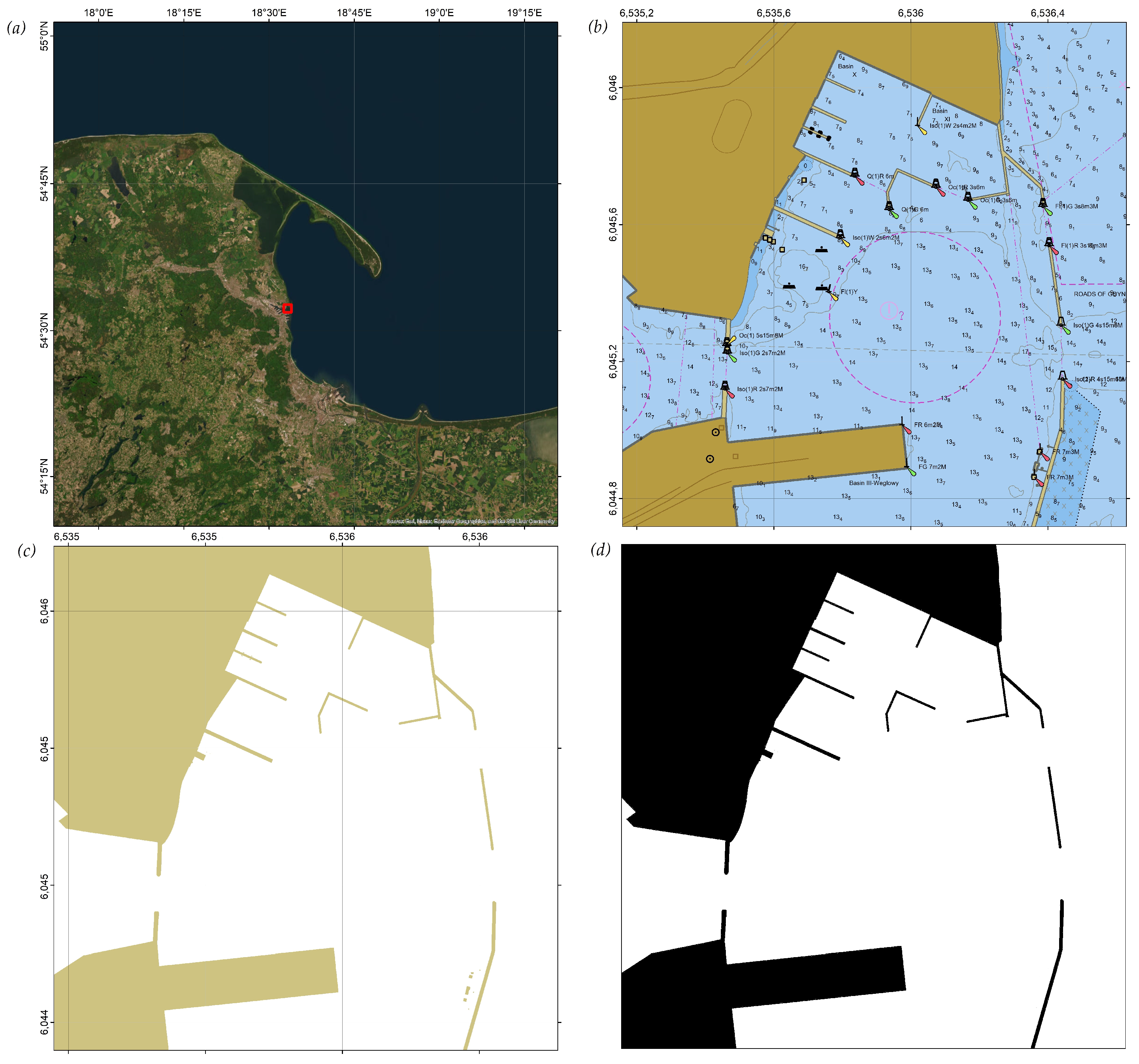
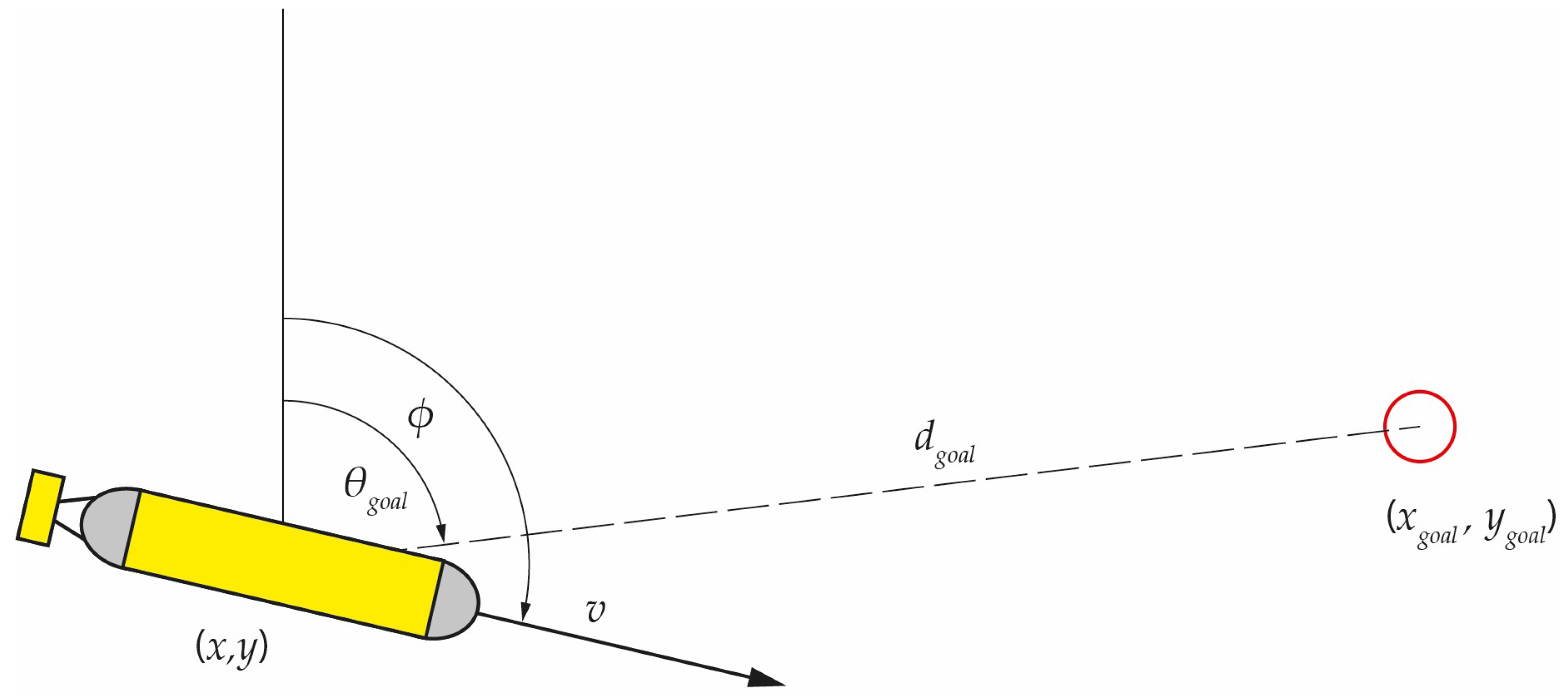
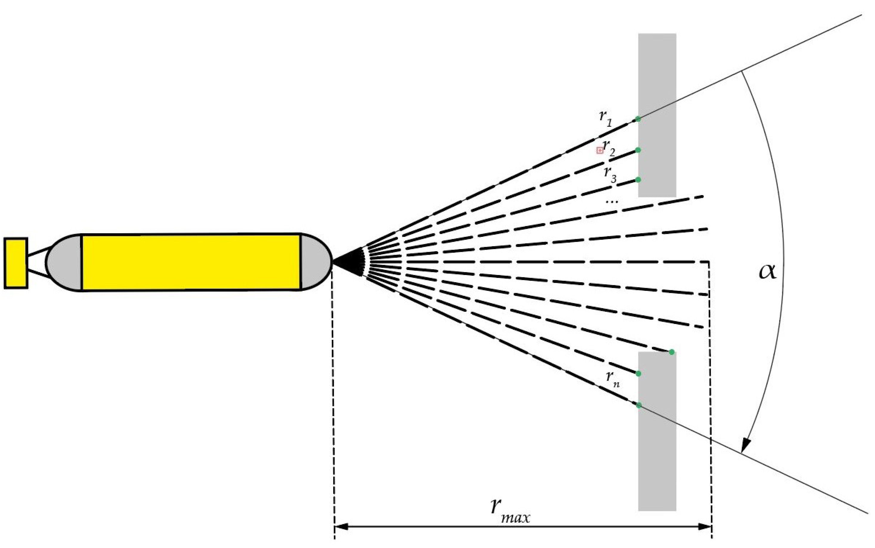
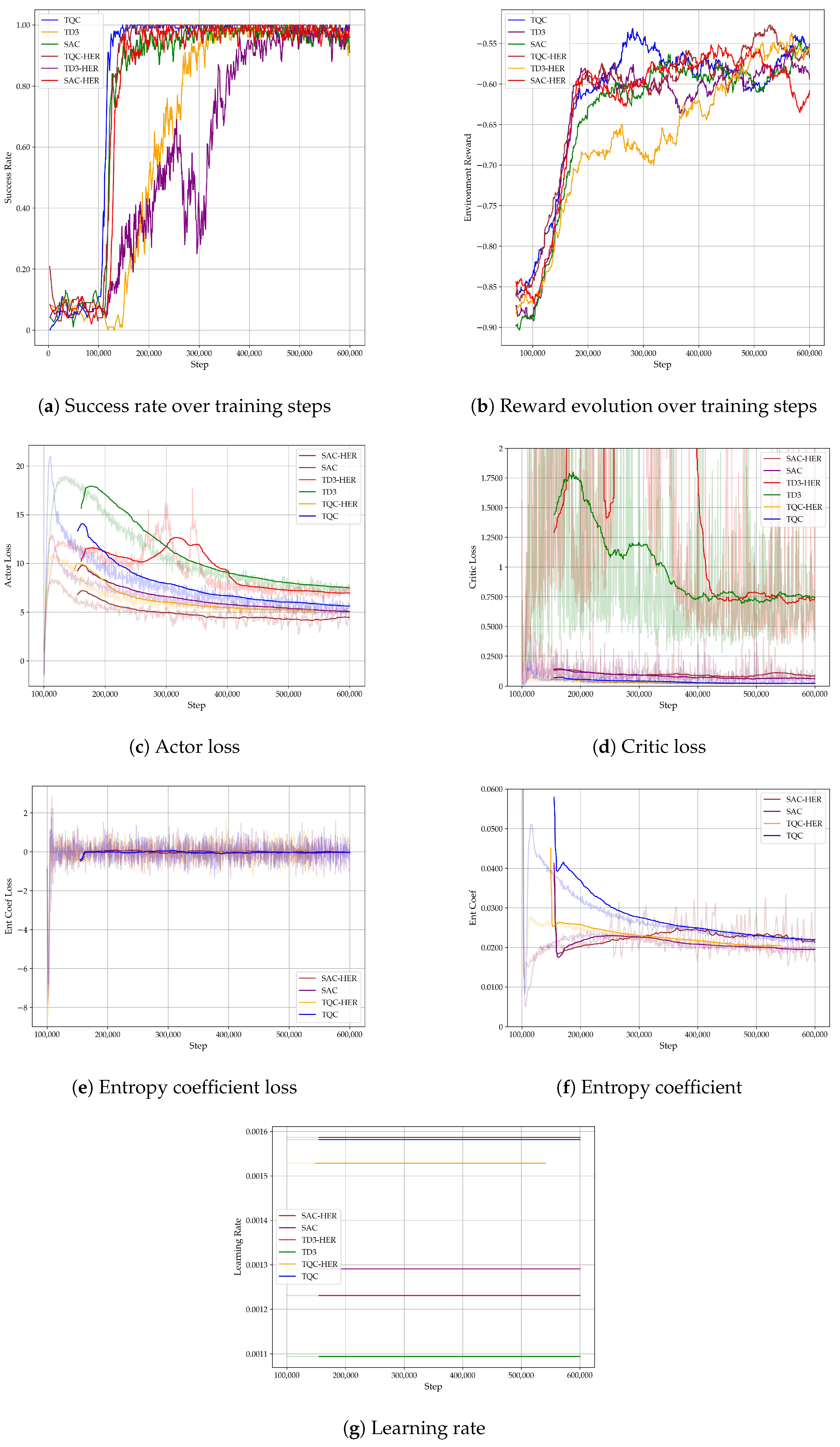
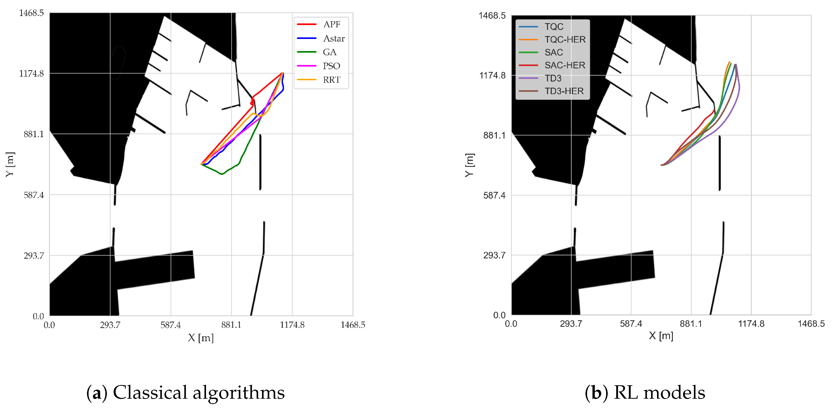
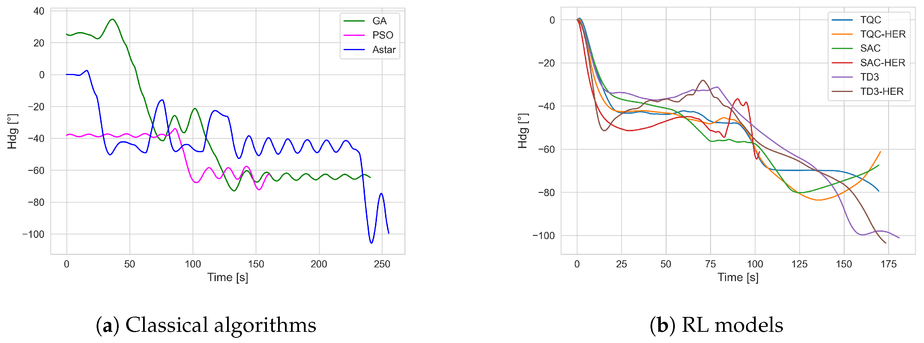
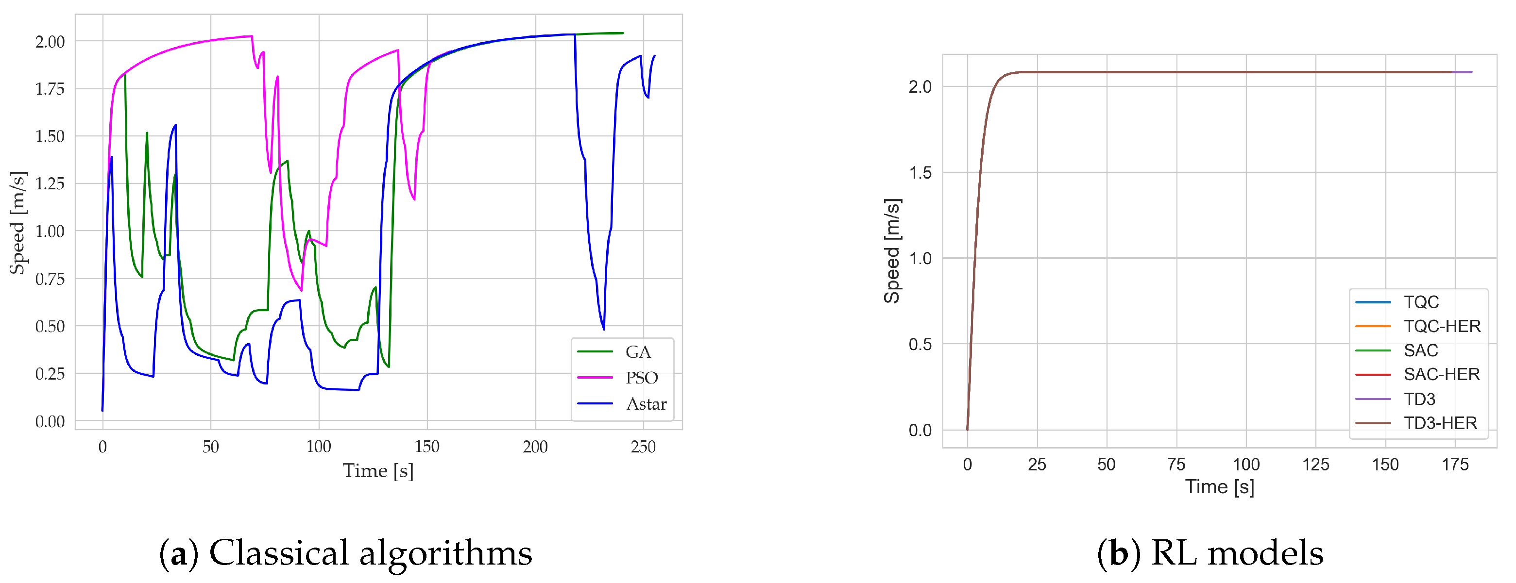
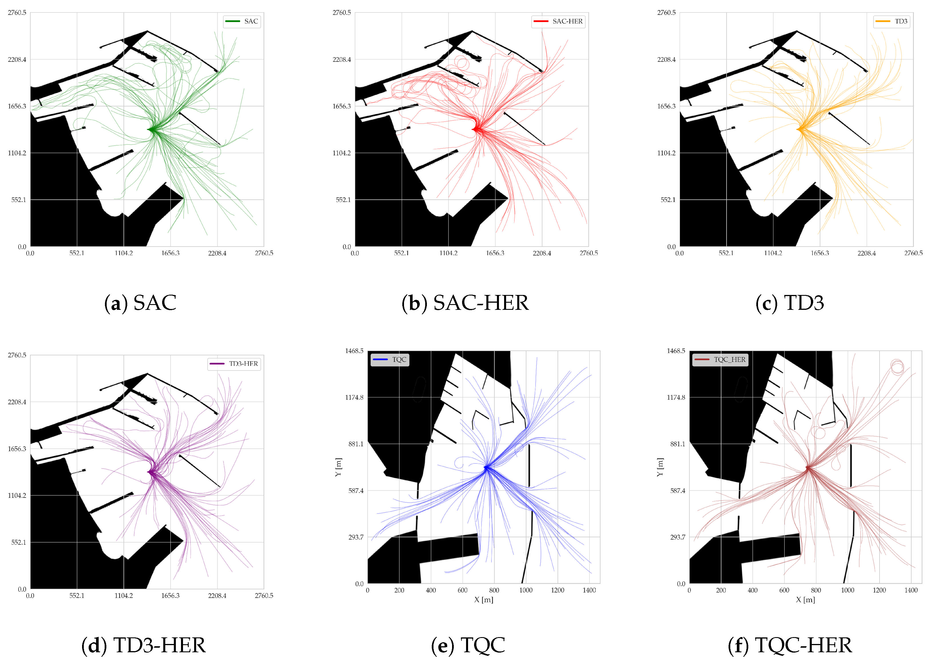