Featured Application
This study provides a hybrid artificial intelligence-based methodology to predict dilution in underground mines.
Abstract
Dilution in underground mining refers to the unintended incorporation of waste material into the ore, reducing ore grade, revenue, and operational safety. Unplanned dilution, specifically, occurs due to overbreak caused by blasting inefficiencies or poor rock stability. To mitigate this issue, various factors related to rock quality, stope geometry, drilling, and blasting must be carefully considered. This study introduces a statistically rigorous methodology for the prediction of dilution in underground mining operations. The proposed framework incorporates a 10-fold cross-validation procedure with 30 repetitions, along with the application of nonparametric statistical tests. A total of eight supervised machine learning algorithms were investigated, with their hyperparameters systematically optimized using two distinct genetic algorithm (GA) strategies evaluated under varying population sizes. The models include support vector machines, neural networks, and tree-based approaches. Using a dataset of 120 samples, the results indicate that the GA-ANN model outperforms other approaches, achieving , , and values of 0.2986, 0.8457, and 0.3928 for the training dataset, and 0.1882, 0.9508, and 0.2283 for the testing dataset, respectively. Furthermore, four stacking models were constructed by aggregating the top-performing base learners, giving rise to ensemble metamodels applied, for the first time, to the task of dilution prediction in underground mining.
1. Introduction
Excavation design in underground mining must predict and control rock displacements within and around excavations to prevent fractures of intact rock, excessive roof and floor deflections, and rock sliding along weakness planes, all of which significantly impact mine stability. Consequently, the stability of underground excavations is closely linked to the stability of their walls, where stope and room characteristics significantly influence overall mine stability. The design of these excavations must anticipate rock mass behavior and consider slope stability, a fundamental aspect of underground mining projects due to their complexity and interdependencies. Additionally, the design must predict dilution, defined as waste rock mixing with ore, thereby reducing its grade. Planned dilution consists of unavoidable waste rock within the stope, whereas unplanned dilution refers to waste rock outside the stope boundaries due to blasting or poor rock stability. Unplanned dilution significantly increases operational costs in underground mining [1,2,3,4]. Figure 1 illustrates various sublevel stoping methods, including drift layouts, drillhole configurations, and differences between designed and actual stope shapes due to overbreak (dilution) and underbreak (ore loss).
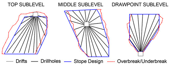
Figure 1.
Different sublevel stoping methods, including drift layouts, drillhole configurations, and variations between designed and actual stope shapes due to overbreak (dilution) and underbreak (ore loss).
Wang [4] states that stope stability and dilution depend on factors such as rock mass classification, in situ stress, stope geometry, blasting techniques, geological structures, and stope exposure time. Empirical [5,6] and numerical methods, such as finite element [7] and boundary element [8] methods, are commonly used to assess dilution and stability in underground excavations. However, both approaches have limitations, e.g., empirical methods do not account for hanging wall geometry, exposure time, blasting effects, and stress variations, while numerical methods may overlook the impact of exposure time, blasting, and rock mass strength properties, depending on the input data [4].
The geological structure of the rock mass, including the location, persistence, and mechanical properties of faults and fractures, is typically assessed using rock quality designation (RQD) [9,10,11]. The most relevant rock mass classification schemes include rock mass rating (RMR) [12,13,14], the Q-system [15], and the geological strength index (GSI) [16,17]. In situ stress evaluation generally involves borehole disturbance, followed by measurements of strain, displacement, or hydraulic pressure. Analytical techniques aid in predicting rock mass responses to mining conditions and proposed stope geometries. Hoek et al. [18] introduced the D factor in the generalized Hoek–Brown criterion to quantify detonation-induced damage to the rock mass. Stope exposure (stand-up) time for unsupported spans can be estimated using the RMR system or the stress reduction factor (SRF) [19].
Various methods are used to design stopes in underground mining and predict stability and dilution. Analytical methods [11,20,21] assess excavation instability based on stress criteria for stress-driven failures and limit equilibrium analysis for structurally controlled failures. However, these methods often yield unrealistic results due to assumptions and simplifications [22]. Numerical modeling [7,23,24] simulates stope mechanical responses but requires an extensive modeling effort, particularly for complex conditions, and relies on accurate rock mass property data. Back analysis [25,26] can enhance numerical modeling accuracy. Empirical tools [5,6,27,28,29], such as the Mathews stability graph method [27], are widely used due to their simplicity but struggle to define stability zone limits objectively. Furthermore, physical modeling using equivalent materials can be employed to emulate the stability of hanging wall rocks, offering a reliable experimental approach that closely mirrors actual dilution phenomena observed during stope development. This technique has proven particularly effective in scenarios involving steeply dipping ore bodies [30,31].
The equivalent linear overbreak slough () concept, introduced by Clark and Pakalnis [28] and Clark [6], quantifies overbreak/slough volumetrically by converting true volumetric measurements into an average depth over the entire stope surface, calculated as follows using Equation (1):
This approach is attractive due to its simplicity and ease of interpretation compared to the use of volumetric measurements. For instance, a 10 m wide stope with an of 1 m corresponds to approximately 10% unplanned dilution. values can be directly measured from post-blast cavity dimensions. Clark and Pakalnis [28] developed a classification scheme to define stability zones based on values, as outlined in Table 1.

Table 1.
Classification of stability zones based on values [28].
Given that dilution results from multiple independent factors, including overbreak and underbreak, statistical, optimization, and artificial intelligence (AI)-based approaches have been developed for its prediction. Germain and Hadjigeorgiou [32] used linear regression to assess relationships between factors such as the powder factor, stope geometry, modified rock mass quality index (Q′), and stope overbreak in a Canadian underground mine. Clark and Pakalnis [28] and Clark [6] proposed four logistic regression models and four artificial neural network (ANN) models to predict in six open stoping operations in Canada, also plotting Mathews graphs from these results. Wang [3] used multi-linear regression analysis (MLRA) to predict based on stress, undercutting, blasting, and stope exposure time in three Canadian underground mines. The study found that exposure time and hydraulic radius (HR) were the most influential factors, followed by the modified stability number (N′) and the stope hanging wall undercutting factor (UF).
Jang and Topal [33] compared the results of four ANN configurations with statistical approaches such as MLRA and multi nonlinear regression analysis (MNRA) models to predict overbreak from underground mines using six independent parameters. Sun et al. [34] developed a wavelet neural network (WNN), a feedforward network with a wavelet transfer function, to predict overbreak in tunnel excavations in China, considering parameters related to the structural plane orientation, trace length, and spacing. Jang [35] and Jang et al. [36] proposed MLRA, MNRA, and a hybrid conjugate gradient algorithm (CGA) with ANN models to predict unplanned dilution and ore loss from three underground long-hole and open stoping mines in Australia, containing information on ten independent variables. The authors used MLRA coefficients to exclude less influential variables, concluding that the CGA-ANN approach outperformed the others. Jang [35] also applied the connection weight algorithm and profile method to assess the influence of independent variables, identifying geology, blasting, and stope design factors as contributing 38.79%, 37.17%, and 24.04%, respectively, with Q′ index and the average horizontal-to-vertical stress ratio (K) being the most influential parameters. Jang [35] and Jang et al. [37] also developed a concurrent neuro-fuzzy system (CNFS) to connect ANN with a fuzzy inference system (FIS), where one model assists the other in decision making, with the FIS being optimized by adjusting fuzzy membership functions (FMF) and fuzzy rules, based on expert knowledge.
Mohammadi et al. [38] employed linear regression and FIS to predict overbreak in tunnel excavation in Iran from nine independent variables. Mohseni et al. [39] proposed a classification system to assess and predict unplanned dilution in the cut-and-fill stoping method, leading to the stope unplanned dilution index (SUDI), which quantifies how susceptible a cut-and-fill stope is to unplanned dilution. Their methodology involved identifying 20 parameters, applying a fuzzy Delphi analytical hierarchy process to assign weights, determining the most influential factors and calculating SUDI to categorize stopes into five classes based on robustness against unplanned dilution. Mottahedi et al. [40] employed MLRA, MNRA, ANN, fuzzy logic, adaptive neuro-fuzzy inference system (ANFIS), and support vector machine (SVM) to predict overbreak from tunnel excavations and mine sites in Iran and India, encompassing five independent variables. Mottahedi et al. [41] extended this research, comparing ANFIS and particle swarm optimization-ANFIS (PSO-ANFIS) models, then confirming the better performance of the PSO-ANFIS model.
Qi et al. [42] applied a random forest (RF) algorithm to predict from a dataset with 13 independent variables obtained from a mine in Australia operating under a transverse open stope mining method with delayed backfill, as provided by Capes [43]. The study formulated the problem as a classification task, categorizing values greater than one as unstable and those below one as stable. The most influential predictors identified were stope dip, stope strike, stope height, rock quality designation (RQD), and joint set number. In a subsequent study, Qi et al. [44] explored multiple machine learning approaches—including logistic regression, ANNs, decision trees (DTs), gradient boosting machines (GBMs), and SVMs—to predict from the same dataset. Additionally, the firefly algorithm (FA) was employed to optimize the hyperparameters of these models, finding that FA-GBM outperformed the other models for the testing set. Building on their previous works and dataset, Qi et al. [45] incorporated techniques such as missing data imputation and semi-supervised learning. The authors optimized the hyperparameters of RF, linear discriminant analysis (LDA), GBM, Gaussian process classification (GPC), SVM, ANN, and logistic regression models using an FA-based metaheuristic. Furthermore, an ensemble model was constructed through a weighted voting approach, thereby surpassing the performance of individual models in terms of classification accuracy.
Jang et al. [46] utilized an ANN to predict uneven break in narrow-vein underground mines in Australia, analyzing a dataset comprising 10 independent variables, with a sensitivity analysis indicating that Q′ and K were the most influential parameters. Expanding on this research, Jang et al. [47] introduced the overbreak resistance factor (ORF) to manage overbreak in tunnel drill-and-blast operations from a tunnel excavation in Japan, incorporating six geological parameters as independent variables. Initially, equal weights were assigned to all variables. Subsequently, five ANN models were trained to predict overbreak, followed by a sensitivity analysis using the profile method. This analysis identified the angle between discontinuities and tunnel contours, as well as the uniaxial compressive strength, as the most significant contributing factors.
Koopialipoor et al. [48] proposed an ANN with a single-hidden layer, alongside a hybrid genetic algorithm-ANN (GA-ANN) model, to predict overbreak in tunnel excavation projects in Iran, incorporating seven independent variables, determining that the GA-ANN significantly outperformed the standard ANN. A subsequent parametric sensitivity analysis identified the rock mass rating (RMR) as the most influential factor in overbreak prediction. Building on this work, Koopialipoor et al. [49] introduced an artificial bee colony-ANN (ABC-ANN) model, leveraging swarm intelligence for optimization and confirming its superior predictive capability when compared to that of standard ANN. Expanding on these findings, Koopialipoor et al. [50] enhanced their approach by developing an ANN with a single-hidden layer trained on an extended dataset incorporating nine independent variables. Additionally, to further optimize blasting parameters and minimize overbreak, the authors employed the ABC algorithm, demonstrating its effectiveness in refining the predictive model and enhancing excavation efficiency.
Zhao and Niu [51] employed an ANN to predict using a dataset comprising samples from six underground mines in China, considering four independent variables, i.e., modified stability number (N′), hydraulic radius (HR), average borehole deviation, and powder factor. Additionally, the authors derived a predictive formula based on the trained model, reaching results superior to those obtained by empirical graph and numerical simulation methods. Bazarbay and Adoko [52] developed two ANN models to predict unplanned dilution in underground mining operations, considering the values of N′, HR, and actual dilution. In addition to model predictions, the authors generated dilution maps based on classification outputs, providing a visual representation of unplanned dilution distribution within mining stopes. Further extending their work, Bazarbay and Adoko [53] proposed an FIS incorporating three membership functions to model the relationship between independent variables (N′ and HR) and unplanned dilution from a mine in Kazakhstan operating under sublevel caving, cut-and-fill stoping, and sublevel stoping mining methods.
Mohseni et al. [54] applied two multicriteria decision-making (MCDM) techniques to assess dilution risk across 10 underground mines in Iran, considering 10 independent parameters. A fuzzy-Delphi analytical hierarchy process was employed to assign relative weights to each parameter; the authors then utilized the multi-attributive approximation area comparison (MABAC) and the technique for order of preference by similarity to ideal solution (TOPSIS) methods to compute a dilution risk score and rank the mines accordingly. The accuracy of these models was validated against actual dilution measurements obtained through a cavity monitoring system, with the MABAC method demonstrating superior precision in classification. Korigov et al. [55] leveraged the same dataset to develop an ANN classification model for predicting unplanned dilution, also introducing probabilistic dilution maps generated from ANN predictions, providing a spatial representation of dilution susceptibility within the evaluated mines. Cadenillas [3] investigated unplanned dilution prediction through both statistical and AI-based regression models from a dataset with 68 parameters from an underground mine in North America, employing the longitudinal retreat long-hole mining method. The study evaluated the predictive capabilities of MLRA, MNRA, ANN, RF, and recurrent neural networks (RNN), and the results indicated that the most influential factors in unplanned dilution were the length and height of the unsupported stope, along with the powder factor, while the RF model achieved the best prediction results.
Jorquera et al. [56] investigated slope stability and dilution prediction using RF, SVM, and k-nearest neighbors (KNN) classification models, analyzing a dataset with nine independent parameters from underground mines in Argentina, Brazil, and Chile, determining that the RF model outperformed the other approaches. He et al. [57] introduced three hybrid versions of RF optimized by nature-inspired metaheuristic algorithms to predict overbreak from a dataset with seven independent variables from a highway tunnel excavation in China. The authors implemented RF models enhanced by the grey wolf optimizer (GWO-RF), the whale optimization algorithm (WOA-RF), and the tunicate swarm algorithm (TSA-RF), indicating the effectiveness of these hybrid approaches in refining RF predictions. Hong et al. [58] developed three hybrid models by integrating the Bayesian optimization (BO) algorithm with existing machine learning methods to enhance overbreak prediction using a dataset from three underground mines in China, incorporating eight independent variables. The authors explored combinations of BO with extreme gradient boosting (BO-XGB), RF (BO-RF), and SVM (BO-SVM), while also comparing them with standard XGB, RF, and SVM models. Among these, BO-XGB demonstrated the best predictive capability for the testing dataset, results that were statistically validated using the Friedman and Wilcoxon signed-rank tests. Additionally, a sensitivity analysis identified tunnel diameter as the most influential factor, contributing 90.5% to overbreak, emphasizing the need for careful control of this variable in tunneling operations.
Liu et al. [59] introduced three hybrid variations of the XGB model—particle swarm optimization-XGB (PSO-XGB), whale optimization algorithm-XGB (WOA-XGB), and sparrow search algorithm-XGB (SSA-XGB)—to predict overbreak in tunnel excavations utilizing a dataset from a tunnel excavation in China, incorporating 12 independent variables. This dataset, originally provided by Zhang [60], was divided into two classes: 48 samples from the upper section (crown to shoulder) and 47 samples from the lower section (shoulder to haunch). For the upper section, the SSA-XGB model outperformed the others for the testing dataset; in contrast, for the lower section, the PSO-XGB and WOA-XGB achieved better performance for the testing dataset. Additionally, the authors implemented a parameter optimization stage to enhance model performance. Expanding on this work, Liu et al. [61] investigated the integration of the SSA algorithm with seven tree-based models: classification and regression tree (CART), RF, gradient boosting decision tree (GBDT), XGB, light gradient boosting machine (LightGBM), categorical boosting (CatBoost), and Deep Forest 21 (DF21), a model derived from the grained cascade forest (gcForest). Using the same dataset as Zhang [60], their analysis confirmed that SSA-XGB consistently outperformed the other models. A feature importance assessment, conducted using the Shapley additive explanation (SHAP) method, revealed the most influential parameters, while an analysis of parameter interactions provided insights into their impact on overbreak prediction. This comprehensive approach led to the development of an optimized parameter tuning method, which successfully reduced overbreak in both the upper and lower sections of the tunnel.
Chimunho et al. [62] employed two hybrid CART models to predict dilution in a sublevel open stoping mine in Australia, characterized by a narrow-to-medium width orebody The authors used a dataset encompassing fourteen independent variables, considering both a complete dataset scenario and its subdivision into two clusters. The first model applied a stepwise selection and elimination (SSE) procedure to identify the most influential parameters before performing CART classification, while the second model utilized principal component analysis (PCA) for dimensionality reduction prior to CART implementation. Under the complete dataset scenario, the SSE-CART model achieved the best accuracy, while the PCA-CART model achieved the best F1-score value, indicating a potential trade-off between dimensionality reduction and predictive robustness. Li et al. [63] introduced a hybrid ANN model incorporating the ant lion optimizer (ALO-ANN) to predict overbreak and underbreak (dilution) in tunnel excavations, utilizing a dataset with 12 independent variables from a tunnel in China. In terms of model architecture, they identified that employing a single-hidden layer with eight nodes significantly enhanced the predictive performance of ALO-ANN. The effectiveness of this model was benchmarked against traditional ANN, generalized regression neural network (GRNN), and extreme learning machine (ELM) models, corroborating the superiority of the ALO-ANN model.
He et al. [64] advanced the ANN framework by integrating deep continual learning techniques, specifically elastic weight consolidation and memory replay (EWC-MR-ANN), alongside an attention mechanism to enhance overbreak prediction. Their study utilized a considerably larger dataset, consisting of 2268 samples with seven independent variables collected from tunnels in China. The dataset was partitioned into ten subsets across five tasks to emulate a multitask and continuous learning scenario. Compared to a conventional ANN, the EWC-MR-ANN demonstrated superior retention of learned parameters across different tasks, thereby mitigating the issue of catastrophic forgetting. While the standard ANN exhibited considerable fluctuations in hyperparameters between tasks, leading to performance degradation, the EWC-MR-ANN maintained stability and exhibited better generalization.
The literature review demonstrates that various AI-based models, including hybrid machine learning models enhanced with metaheuristics, have been successfully applied over the past decades to predict dilution in underground mines. Hyperparameter tuning is a critical step in ML applications, as traditional methods like grid search offer a limited capacity for exploring the hyperparameter space. By formulating this process as an optimization problem and leveraging population-based metaheuristics, the likelihood of identifying an optimal hyperparameter configuration that minimizes training error is significantly increased.
Nevertheless, future research in this domain could benefit from the exploration of alternative methodologies. While He et al. [64] proposed a framework to simulate a continual learning environment—an important consideration given the inherently static nature of most supervised machine learning implementations—the task of predicting dilution in underground mining operations has yet to be formally addressed from a time series modeling perspective [65]. Additional machine learning paradigms, such as radial basis function networks (RBNs) and adaptive boosting (AdaBoost) algorithms, remain underexplored in this context and may offer enhanced predictive performance [66,67]. Ensemble techniques, particularly stacking, also hold promise for improving accuracy through the aggregation of multiple base learners into a more robust metamodel [68]. Moreover, a critical limitation of many existing studies lies in their insufficient statistical grounding, often lacking rigorous explanation or validation of the results obtained. Given the stochastic behavior and sensitivity of most machine learning models to variations in the data, the implementation of nonparametric statistical tests should be encouraged to assess whether observed differences in performance are statistically significant [69].
This study introduces a practical framework for predicting dilution () in underground mining using ML models in combination with genetic algorithms (GAs). The proposed pipeline effectively addresses variable distribution skewness and is designed for implementation even on domestic computing systems. The principal contribution of this work resides in the implementation of a stacking-based artificial intelligence model—an ensemble learning strategy that synthesizes multiple base learners into a single, more generalized metamodel—for the prediction of dilution. To the best of the authors’ knowledge, this represents the first application of such an approach for this specific task. In addition, the study adopts a rigorous statistical framework that may serve as a methodological reference for future research aiming at greater robustness in predictive modeling. A stratified sampling strategy is employed to preserve the original distribution of the target variable across training and testing datasets, mitigating potential biases due to data imbalance. During the hyperparameter tuning phase, each ML-based model was optimized using genetic algorithms configured with multiple population sizes, thereby leveraging the stochastic nature of these metaheuristics. A repeated k-fold cross-validation scheme was applied to enhance the reliability of the performance evaluation. Furthermore, the training dataset was subjected to a 10-fold cross-validation procedure with 30 repetitions to derive robust validation metrics. Finally, nonparametric statistical tests were conducted to verify whether the observed superiority of certain models in the training and testing stages remained statistically significant under validation. Collectively, these methodological elements underscore the statistical soundness and reproducibility of the proposed framework, rendering it a solid foundation for future investigations in this domain.
The remainder of this paper is structured as follows: Section 2 details the materials and methods employed, covering the regression models and GAs; exploratory data analysis; the training, testing, and validation framework; as well as statistical tests. Section 3 presents the results obtained from the numerical experiments and provides a discussion of these findings. Finally, Section 4 outlines the conclusions and potential future directions to enhance the study’s main contributions. A comprehensive list of abbreviations employed throughout this paper is provided in Appendix A.
2. Materials and Methods
2.1. Regression Models and Genetic Algorithm
In this study, dilution () prediction is addressed as a regression problem, in which the hyperparameters of the machine learning (ML) models are tuned using genetic algorithms to optimize their predictive performance.
2.1.1. Neural Networks: Artificial Neural Network and Extreme Learning Machine
Building upon the foundational work of McCulloch and Pitts [70], Rosenblatt [71], and Rumelhart et al. [72], artificial neural networks (ANNs) represent independent variables as nodes (neurons) in an input layer and dependent variable(s) as nodes in an output layer, with hidden layers in between to model nonlinear relationships. Each node in a layer connects to all nodes in adjacent layers, with assigned weights. ANNs use feedforward architectures trained via backpropagation, adjusting weights iteratively through gradient-based optimization methods. Activation functions transform the weighted inputs in the hidden layers into predictions, and biases enhance generalization. Despite their robustness and parallelizability, ANNs require careful architecture tuning and often display low learning efficiency.
Huang et al. [73] introduced the extreme learning machine (ELM) as an alternative, using a single-hidden layer where weights and biases are randomly assigned and fixed, avoiding iterative gradient descent. Only the weights between the hidden and output layers are adjusted. This method significantly accelerates training but is susceptible to instability, poor generalization, and sensitivity to outliers and imbalanced data.
2.1.2. Support Vector Machine
Vapnik and Chervonenkis [74] developed the support vector machine (SVM) to solve classification tasks by defining the hyperplanes that best separate data points. In high-dimensional spaces, these hyperplanes act as decision boundaries; maximizing the margin between points ensures optimal separation. Vapnik et al. [75] extended this concept to support vector regression (SVR), which approximates nonlinear functions via linear splines. SVM and SVR models generalize well, handle both linear and nonlinear problems effectively, and use kernel functions for complex transformations. However, their performance is limited when dealing with large datasets due to computational complexity.
2.1.3. Tree Models: Decision Tree, Random Forest, and Extreme Gradient Boosting
Decision trees (DTs) are hierarchical models introduced by Morgan and Sonquist [76], applicable to both classification and regression tasks. A DT consists of a root node, internal decision nodes, and terminal leaf nodes. It follows a divide-and-conquer strategy, recursively splitting data until achieving homogeneous subsets. While effective, DTs tend to overfit, necessitating pruning techniques to eliminate redundant branches. Breiman [77] proposed the random forest (RF) model as an ensemble of DTs that aggregates predictions from multiple subtrees trained on different data subsets. RF improves robustness and generalization but increases computational cost and reduces interpretability.
Tree-boosting techniques combine multiple weak learners sequentially, refining predictions iteratively. Gradient boosted decision trees leverage gradient descent to minimize residual errors. Chen and Guestrin [78] introduced extreme gradient boosting (XGB), a highly scalable tree-boosting algorithm that employs parallel computation, regularization, and sparsity-aware learning to handle missing data. Despite its strong predictive capabilities, XGB is computationally expensive and prone to overfitting with excessive trees or small datasets. Further details on these models can be found in the work of Raschka et al. [66].
2.1.4. Model Hyperparameters
The predictive performance of machine learning (ML) models is highly sensitive to the configuration of their hyperparameters, making hyperparameter tuning a critical and often complex stage in model development. This process involves navigating a high-dimensional and frequently non-convex search space, which renders it computationally intensive and potentially prone to suboptimal convergence. While approaches such as greedy search and population-based metaheuristic algorithms are commonly adopted, they can exhibit limitations in regards to convergence speed and efficiency. Not all hyperparameters contribute equally to a model’s performance; hence, the selection of which parameters to tune must be made judiciously. For instance, in artificial neural networks, hyperparameters such as learning rate, number of hidden layers, and number of neurons per layer are known to directly affect both convergence rate and predictive accuracy. Similarly, in tree-based models like decision trees and random forests, key hyperparameters—including maximum tree depth, minimum number of samples per leaf, and the number of trees—govern model complexity and generalization capacity [79,80]. Figure 2 illustrates the hyperparameters of these models subjected to tuning procedures, where square brackets [ ] indicate real number ranges and curly brackets { } indicate categorical or integer domains.
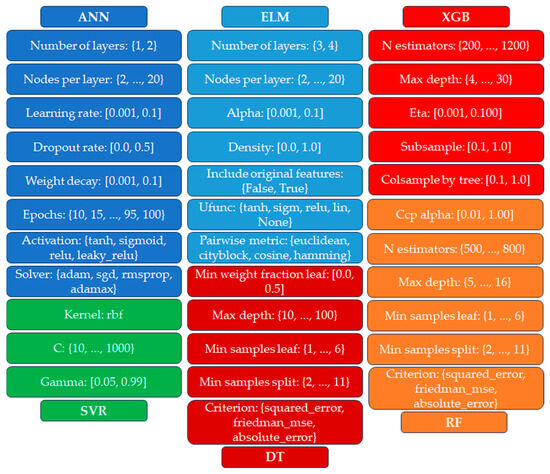
Figure 2.
Hyperparameters of the models used in this study, subjected to tuning procedures.
2.1.5. Stacking
Wolpert [68] introduced stacking as an ensemble learning technique that combines multiple base models (level 0) into a higher-level metamodel (level 1) to enhance generalization. The base models generate predictions, which serve as input for the metamodel. Cross-validation mitigates overfitting, and a holdout dataset improves the final model’s robustness. While stacking typically outperforms the results of individual models, its success depends on the diversity and performance of the base models and requires increased computational resources.
2.1.6. Metrics
The predictive performance of the models is evaluated using the coefficient of determination (), mean absolute error (), and root mean square error (), defined by Equations (2)–(4) as follows:
where and represent the actual and predicted values, respectively, and denotes the total number of samples.
2.1.7. Genetic Algorithms
To optimize the hyperparameters of the models, a genetic algorithm (GA) was integrated into the training process. Originally developed by Holland [81], GA is a population-based metaheuristic and an evolutionary algorithm inspired by Darwinian evolution. Over multiple generations, the fittest individuals prevail, gradually refining solutions to optimization problems. A standard GA consists of defining an initial population, evaluating each individual’s fitness function, selecting parents, performing crossover to generate offspring, and applying mutation to introduce variability. These newly generated offspring then serve as parents for the next generation.
In a GA, each chromosome represents a potential solution where variables are arranged sequentially. Continuous variables are typically encoded in binary form, requiring decoding to compute the fitness function, while discrete variables assume predefined values without encoding. Due to these characteristics, continuous and discrete hyperparameters must undergo different mutation and crossover operations.
In this study, the GA was executed for a maximum of 100 generations in all experiments, with five different population sizes tested for each ML model: 20, 35, 50, 65, and 80 individuals. The fitness function was defined using the mean absolute error (), ensuring that lower values represented superior hyperparameter configurations. Continuous hyperparameters were encoded using 8-bit binary representation. Parent selection was performed via a tournament of three randomly chosen individuals, with replacement into the selection pool. Crossover for continuous hyperparameters followed a two-point strategy with a probability of 0.90, while mutation was applied by flipping a binary allele with a probability of 0.10. For discrete hyperparameters, crossover involved swapping alleles between parents with a probability of 0.30, while mutation randomly replaced an allele with another feasible value with a probability of 0.10.
Figure 3 illustrates an example of a chromosome representing one encoded continuous hyperparameter and two discrete hyperparameters, while Figure 4 presents a flowchart of the GA process used to optimize model hyperparameters.
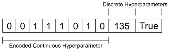
Figure 3.
Example of a chromosome representing one encoded continuous hyperparameter and two discrete hyperparameters.
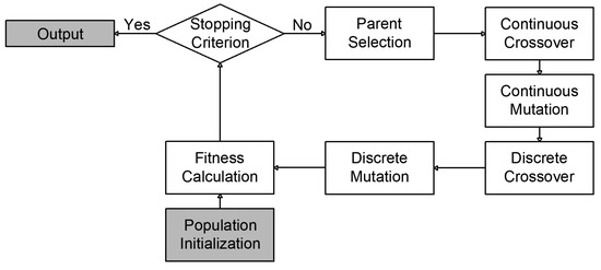
Figure 4.
Flowchart of the genetic algorithm used to optimize model hyperparameters.
In addition to the standard GA, an adaptive genetic algorithm (AGA) was implemented. This variant maintains the fundamental structure of GA but incorporates two key enhancements: an elitism mechanism and dynamically adjusted probabilities for crossover and mutation. The adaptive probability mechanism follows Equation (5):
where represents the current iteration (generation), is the total number of iterations, is the operator probability at iteration , and and denote the upper and lower bounds for the probability, respectively.
By adapting the probabilities throughout the evolution process, the AGA prioritizes exploration in the early generations and progressively shifts towards exploitation as the population converges. This controlled transition helps balance diversity and convergence efficiency. Furthermore, an elitism operator was included to ensure that the best individual found so far is retained in the current population. After applying genetic operators and computing fitness values, the worst-performing individual is replaced by the best-performing individual from the previous generation.
For the AGA in this study, the probability of continuous crossover and mutation ranged from 0.50 to 0.90 and from 0.05 to 0.20, respectively, while the discrete crossover and mutation probabilities ranged from 0.10 to 0.30 and from 0.01 to 0.10, respectively. Figure 5 provides a flowchart illustrating the AGA process employed for hyperparameter tuning.
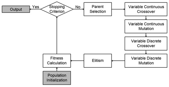
Figure 5.
Flowchart of the adaptive genetic algorithm employed for hyperparameter tuning.
2.2. Exploratory Data Analysis
Exploratory data analysis (EDA) is a critical step in any supervised machine learning (ML) workflow. Due to the sensitivity of AI-based models, it is essential to properly scale variables, understand their distributions, and detect potential noise or outliers. Another fundamental aspect of EDA is feature importance analysis. Given the curse of dimensionality, providing excessive input features can lead to increased computational costs and degraded model performance. Dimensionality reduction through feature selection helps mitigate these issues by prioritizing only the most relevant predictors. Additionally, feature engineering can enhance learning efficiency by creating new informative variables while avoiding collinearity.
The dataset used in this study was obtained from Zhao and Niu [51], consisting of 120 samples with five independent variables: modified stability number (N′), hydraulic radius (HR (m)), mean borehole deviation (BD (m)), powder factor (PF (kg/t)), and equivalent linear overbreak slough ( (m)). These parameters are relevant because they address aspects related to the rock mass classification, stope geometry, drilling, and blasting—fundamental factors for assessing stope stability and predicting dilution, as stated by Wang [4]. As previously mentioned, simulation-based and empirical methods often overlook or oversimplify some of these variable classes. Therefore, the dataset employed in this study offers a comprehensive and suitable foundation for the application of supervised machine learning techniques, allowing for more accurate and data-driven predictions. In the supervised learning context, serves as the dependent variable (target y), while the remaining features comprise the independent variable set X.
2.3. Tuning Model Hyperparameters
Following the exploratory data analysis stage, a random seed was generated and stored to ensure reproducibility. The dataset was then categorized into classes, as outlined in Table 1, to maintain the robustness of the subsample distributions. A stratified sampling approach was applied, dividing the dataset into training and testing subsets in a 5:1 ratio, ensuring that both subsets preserved the statistical properties of the original distribution.
Given that distribution skewness and statistical outliers can hinder model training, and considering that independent variables typically exhibit varying scales—where larger numerical values might be incorrectly interpreted as more important than smaller ones—it was necessary to apply an appropriate distribution transformation. Since different machine learning models respond variably to different transformations, standard scaling, robust scaling, and power scaling were evaluated. The selected transformation was fitted to the X_train dataset and subsequently applied to both the X_train and X_test datasets, ensuring that the transformation parameters were learned solely from the training data. Additionally, the impact of transforming the y_train target variable was assessed for each model to determine whether it contributed to improved learning performance.
Each AI-based model was trained using a genetic algorithm (GA) to optimize the set of hyperparameters outlined in Figure 2. To ensure reliable model evaluation and prevent overfitting, a 5-fold cross-validation procedure was applied during the training phase. The optimization objective was to minimize the mean absolute error (), thus guiding the GA toward hyperparameter configurations that enhance predictive accuracy. To enhance the robustness of the results, the entire cross-validation process was repeated five times, with the data being randomly shuffled before each iteration. The final score for each hyperparameter configuration was computed as the average across all folds and repetitions.
Given that each set of hyperparameters is represented as a chromosome within the genetic algorithm framework—similar to the example illustrated in Figure 3—this entire training procedure was executed for each individual across all generations. Consequently, multiple hyperparameter configurations were evaluated for each model, and in each generation, the best-performing individual (i.e., the hyperparameter set yielding the lowest ) was stored. This iterative optimization process ultimately yielded the optimal hyperparameter configuration for each model in the studied training dataset. Pseudocode 1 provides a representation of the hyperparameter tuning procedure.
| Pseudocode 1. Hyperparameter tuning procedure. |
| Input: A dataset with independent () and dependent () variables; a genetic algorithm ; AI-based models; hyperparameters; . Exploratory data analysis: Checking for the presence of noise data and outliers, identifying the important variables, and performing feature engineering, if necessary. Training and tuning the models: Random generation and storage. Stratification of (5/6 samples); (1/6 samples). Fitting and Transformation of (and , if necessary). Transformation of (and , if necessary). Regardless of whether there is a transformation or not, they will be called and here. Let be the AI-based models, be the hyperparameters of , be the population size, and be the repetitions, where . For : For : For : . end . end . end Output: . |
2.4. Training, Testing, and Validation Metrics
For each machine learning model and its corresponding best set of hyperparameters, the , , and metrics were computed for both the training and testing datasets. This procedure entails subjecting the data subsets to the trained models once their hyperparameter configurations have been finalized, thereby simulating model performance for previously unseen data. Naturally, models tend to exhibit strong performance for the training dataset, as their hyperparameters are optimized based on that data. However, it is imperative that they also demonstrate high predictive accuracy using the testing dataset, which remains completely excluded from the training process. Failure to generalize well to this unseen subset indicates a lack of robustness and a tendency toward overfitting.
These experiments provide insight into the generalization ability of the models when applied to unseen data and serve as indicators of underfitting or overfitting. Additionally, the training dataset underwent a 10-fold cross-validation procedure with 30 repetitions, allowing for the retrieval of validation metrics. This step ensures a more comprehensive statistical evaluation of model performance and assesses model robustness against variations in input data. The overall workflow for obtaining training, testing, and validation metrics is illustrated in Pseudocode 2.
| Pseudocode 2. Training, testing, and validation of the machine learning models. |
| Input: ; (or ); ; (or ); all ; ; . Regardless of whether there is a transformation or not, they will be called and here. Training and Testing Metrics: For : Back Transformation of the data. . . end Validation Metrics: Let be the repetitions, where . For : For : . end . end Output: ; ; . |
Given that the proposed methodology generates 10 distinct hyperparameter sets for each machine learning model—five derived from different population sizes in GA and five from different population sizes in AGA—it was necessary to define a selection criterion to determine the best overall configuration. For each genetic algorithm (GA and AGA), the optimal hyperparameter set was determined based on the following ranking criteria:
- Lowest value (primary criterion).
- Highest value (secondary criterion, used in case of a tie).
- Lowest value (tertiary criterion, used if the first two metrics are identical).
- Smallest population size (if all three performance metrics remain tied).
When selecting between the best configurations obtained from both GA and AGA, the same hierarchical criteria were applied. If the performance of the top models from GA and AGA remained identical across all metrics, the hyperparameters obtained via GA were arbitrarily selected.
The computed training and testing metrics for each model—optimized through GA and AGA—are presented in Appendix B. All validation metrics reported in this study represent the mean values across different folds, accompanied by their corresponding standard deviations, ensuring a statistically robust evaluation of model performance.
2.5. Stacking Models Using Ridge Regressor
To leverage the strengths of multiple machine learning models and enhance predictive performance, a stacking ensemble approach was employed. This method integrates the predictions from multiple base models as inputs into a metamodel, which learns to optimally combine these predictions to produce a final, more robust output. In this study, a ridge regressor was selected as the metamodel, and a 10-fold cross-validation procedure with 30 repetitions was applied to mitigate overfitting. Given that different base models may capture similar patterns in the data, their predictions tend to be correlated. The ridge regressor was chosen as the metamodel due to its ability to handle multicollinearity among base model predictions. By incorporating an L2 penalty term into its cost function, the ridge regressor shrinks the coefficients towards zero, reducing model variance and improving generalization capacity. Additionally, it is computationally efficient and requires the tuning of only a single hyperparameter (alpha).
To systematically evaluate the impact of different model combinations, four stacking configurations were proposed:
- Stacking 1: uses the two best base models.
- Stacking 2: uses the three best base models.
- Stacking 3: uses the four best base models.
- Stacking 4: uses the five best base models.
To ensure a fair comparison, each ML-based model—selected based on its optimal hyperparameters—was benchmarked against these four stacking configurations. The training, testing, and validation performances of these stacking models were evaluated following the same validation methodology described in the previous section. The workflow for constructing, training, testing, and validating the stacking models is presented in Pseudocode 3.
| Pseudocode 3. Building, training, testing, and validation of the stacking models. |
| Input: ; (or ); ; (or ); all ; ; . Regardless of whether there is a transformation or not, they will be called and here. Stacking: Let be the metamodels to be built. For : A certain number of the best models in . . end Training and Testing Metrics: For : Back Transformation of the data. . . end Validation Metrics: Let be the repetitions, where . For : For : . end . end Output: ; ; ; . |
2.6. Nonparametric Statistical Tests
To account for the stochastic nature of the proposed pipeline, nonparametric statistical tests were employed to determine whether a model’s performance is statistically superior to that of other models, based on the validation dataset metrics. The Friedman test [82] is a widely used nonparametric statistical test designed to detect differences in performance across multiple trials when the same subjects (datasets) are exposed to different treatments or conditions, such as predictions from various ML-based models. This test ranks the performance of each model per dataset and then compares the average ranks across models to assess whether statistically significant differences exist. In the case of tied ranks, average ranks are assigned.
Given that represents the rank of the model among models on the the dataset out of datasets, the Friedman test computes the average rank of each model using . Under the null hypothesis (), which assumes all models perform equivalently, the Friedman test statistic is calculated as Equation (6):
This statistic follows a Chi-square distribution with degrees of freedom when and . If the null hypothesis is rejected (), it indicates a statistically significant difference in model performance. In such cases, Nemenyi’s post hoc test [83] is applied for pairwise model comparisons to identify which models perform significantly better. A statistically significant difference between two models is established if their average ranks differ by at least the critical difference (), which is computed as Equation (7):
where (typically consider ) is derived from the Studentized range distribution divided by . By employing these statistical tests sequentially, it is possible to rank the models and determine whether a particular model consistently outperforms the others, identifying whether a clear “champion” model exists, based on statistically significant differences.
For more information, the procedures described by Demsar [69] could be consulted.
Once the final hyperparameter configurations for all models were determined, their validation performances (, , and ) across 30 repetitions of the 10-fold cross-validation procedure were subjected to the Friedman test to verify whether the null hypothesis is rejected. If so, the Nemenyi test was applied for pairwise comparisons. The results of these pairwise comparisons allowed for the ranking of the models based on their win counts across different interactions, helping to determine the best-performing models—provided that their differences exceed the threshold. Pseudocode 4 outlines the nonparametric statistical test procedure.
| Pseudocode 4. Nonparametric statistical test procedure. |
| Input: all , ; all , ; . . . Pairwise Testing Comparison: Let be the , , and metrics, and be the probability value for the metric . For : . If : For : . end . end end Output: . |
2.7. General Comments
All machine learning models employed in this study were implemented in Python 3.12.7, leveraging various specialized libraries for different stages of the pipeline. The exploratory data analysis (EDA) was conducted using the scikit-learn library, employing tools such as train_test_split for dataset partitioning, StandardScaler and PowerTransformer for data transformation, and RepeatedKFold for cross-validation. These techniques ensured robust preprocessing and statistical consistency across different model training procedures.
For model implementation, the study utilized a combination of libraries:
- scikit-learn: implemented the SVR, DT, RF, XGB, and stacking models.
- skelm: employed for the ELM model.
- PyTorch 2.6.0: used to construct the ANN model.
All hyperparameters not explicitly tuned in this study were set to their default values as defined in their respective libraries. The genetic algorithm (GA) models were developed from scratch, ensuring a high degree of customization and flexibility in tuning machine learning hyperparameters. Additionally, statistical tests were conducted using the SciPy library to ensure rigorous performance evaluation and model comparison.
The numerical experiments were performed on a laptop running Windows 10 (2022), equipped with the following:
- Processor: 11th Gen Intel(R) Core i7-1165G7 @ 2.80 GHz.
- Storage: 500 GB SSD.
- Memory: 16 GB RAM.
This computational setup was sufficient to train, evaluate, and validate all models, ensuring efficient execution of the hyperparameter tuning process, statistical tests, and performance comparisons.
3. Results and Discussion
3.1. Exploratory Data Analysis Results
To assess the relevance of independent variables for training the machine learning models, Spearman′s correlation coefficient was calculated between each independent variable and the target variable () using the dataset provided by Zhao and Niu [51]. The dataset comprises 120 samples and four continuous independent variables: N′ (modified stability number); HR (hydraulic radius); BD (mean borehole deviation); and PF (powder factor). The computed Spearman correlation coefficients with are as follows:
- N′: −73% (strong negative correlation).
- HR: 35% (moderate positive correlation).
- BD: 23% (weak positive correlation).
- PF: −20% (weak negative correlation).
Since there are no discrete variables in this dataset, all features are treated as continuous.
Figure 6 and Figure 7 provide an in-depth visual representation of the dataset characteristics. Figure 6 displays violin plots, which illustrate the distribution density of each variable, and Figure 7 presents a correlation heatmap, scatterplots, and histograms for all variables, helping to visualize relationships, potential collinearity, and distribution skewness.
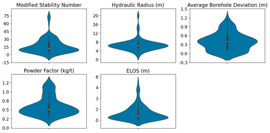
Figure 6.
Violin plots of the variables.
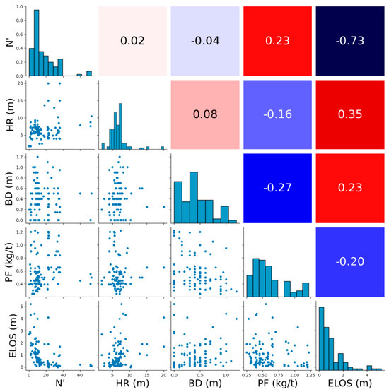
Figure 7.
Correlation heat map (negative and positive correlations are represented in cool and warm colors, respectively), scatterplots, and histograms of all variables.
The variable scales differ significantly, which could introduce biases during model training if not properly handled. Right-skewed distributions are observed for some variables, including the target variable (), where higher values deviate substantially from the mean. This skewness and variance disparity indicate the necessity of applying distribution transformations to ensure that the data presents a smoother behavior, ultimately improving the ability of ML models to learn and generalize effectively. To address these issues, various data transformation techniques, such as standard scaling, robust scaling, and power transformations, were evaluated, aiming to enhance model interpretability and predictive performance.
3.2. Hyperparameter Tuning and Metrics for Training, Testing, and Validation
After completing the exploratory data analysis, various scaling techniques—standard, robust, and power scaling—were tested on the X_train and y_train datasets to improve model performance. It was found that applying the Yeo–Johnson [84] transformation significantly enhanced model accuracy, as this technique transforms data into a more Gaussian-like distribution, reduces high variance and skewness, and improves symmetry in variable distributions, making it easier for models to learn effectively.
Following the data transformation, a random seed was fixed to ensure reproducibility before splitting the dataset. The next step involved optimizing the hyperparameters of the machine learning models using genetic algorithms. Table 2 compares the computational time required for hyperparameter tuning across different models. In total, 37,778 min were consumed in this stage. The least time-consuming models were DT (0.12%), ELM3 (0.20%), and ELM4(0.30%), while SVR (0.27%), ANN1 (7.78%), and ANN2(8.88%) consumed a moderate amount of time. The most time-consuming models were XGB (21.44%) and RF (61.02%), indicating a significantly higher computational burden.
Table 2.
Comparison of the computational time during the hyperparameter tuning experiments.
Figure 8 and Figure 9 illustrate the performance of the best hyperparameter configurations for each machine learning model, while Table 3 summarizes their training and testing performance.
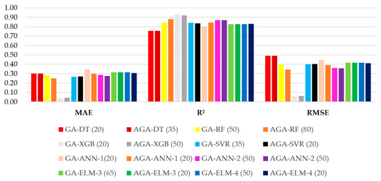
Figure 8.
Training metrics for the best machine learning models.
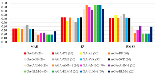
Figure 9.
Testing metrics for the best machine learning models.
Table 3.
Training and testing metrics for the best set of hyperparameters determined for each machine learning model.
As illustrated in Figure 8, the models demonstrated relatively consistent behavior for the training dataset with respect to the metric, yielding values ranging from 0.7579 to 0.9321. In contrast, greater variability was observed for the and metrics, which ranged from 0.0396 to 0.3426 and from 0.0576 to 0.4920, respectively. The GA-XGB model with a population of 20 individuals produced the most favorable training metrics overall. Conversely, the GA-ANN-1 model with 20 individuals exhibited the highest , while both decision tree-based models recorded the lowest and highest values.
Referring to Figure 9, the testing dataset results reveal a broader spread in model performance, particularly for the metric, which ranged from 0.3981 to 0.9544. The values ranged from 0.1882 to 0.4354, while the values ranged from 0.2197 to 0.7153. Notably, the AGA-ANN-1 model with 20 individuals yielded the lowest on the testing dataset, at 0.1882. The highest values were attained by three extreme learning machine-based models—GA-ELM-3 with 65 individuals, AGA-ELM-3 with 20 individuals, and GA-ELM-4 with 50 individuals. With respect to , the best results were shared by the AGA-ELM-3 with 20 individuals and GA-ELM-4 with 50 individuals models, both of which demonstrated superior generalization performance on the testing dataset.
According to the selection criterion defined in the methodology, the AGA-ANN-1 model with a population of 20 individuals was identified as the most effective. This model achieved , , and values of 0.1882, 0.9508, and 0.2283, respectively, for the testing dataset. As shown in Table 3, its performance on the training dataset was also satisfactory, with corresponding values of 0.2986, 0.8457, and 0.3928, indicating a consistent behavior across both data partitions and confirming the robustness of the model for the problem at hand.
Overall, all neural network models—both traditional artificial neural networks (ANNs) and extreme learning machines (ELMs)—exhibited excellent predictive capability across training and testing sets. Their values ranged from 0.1882 to 0.2765, values spanned from 0.8327 to 0.9544, and values varied from 0.2197 to 0.4210, further reinforcing the superior generalization ability of neural-based approaches for the dataset under investigation.
A noteworthy observation concerns the moderate performance of the extreme gradient boosting (XGB) models for the testing dataset, despite their outstanding results for the training dataset—an indication of overfitting. Similarly, the random forest (RF) models exhibited a significant drop in predictive performance from training to testing, suggesting that they too may have been affected by overfitting. Conversely, among the tree-based models, the decision tree (DT) models—although presenting the weakest results during training—achieved the most favorable testing metrics, implying a more robust generalization under the specific conditions evaluated, in contrast to their more complex counterparts.
Regarding the support vector regressor (SVR) models, their performance mirrored that of the RF models, with a notable reduction in accuracy from training to testing. Nevertheless, the gap in between training and testing was smaller than that observed for the RF models, indicating relatively greater stability. A detailed comparison of the mean validation metrics for the best-performing models is provided in Table 4.
Table 4.
Mean validation metrics for the best set of hyperparameters determined for each machine learning model.
In these experiments, the mean values ranged from 0.3534 to 0.4623. The three best-performing models in this regard were GA-ELM-4 (50), AGA-ELM-3 (20), and AGA-SVR (20), once again highlighting the effectiveness of the ELM architecture, while also drawing attention to the solid performance of the SVR model, despite its less impressive results on the testing dataset. Regarding the metric, values varied from 0.4850 to 0.7466, with the highest scores obtained by GA-ELM-4 (50), AGA-ELM-3 (20), and GA-ELM-3 (65), reaffirming the dominance of neural network-based models in capturing the variance of the target variable.
As for , the results fell between 0.3954 and 0.6233. Interestingly, the top three performers under this metric were GA-SVR (35), GA-ELM-4 (50), and GA-ELM-3 (65), with the SVR model outperforming its ELM counterparts in terms of error magnitude. Although artificial neural networks (ANNs) did not rank among the top three models for any of the evaluated metrics, they still delivered consistently strong and reliable performance, indicating their robustness across different validation scenarios.
With respect to tree-based models, their validation performance was significantly lower than that of the SVR and neural network-based models. Among the tree-based approaches evaluated, the random forest (RF) models consistently outperformed both decision tree (DT) and extreme gradient boosting (XGB) variants across the three validation metrics considered (, , and ). In contrast, DT models exhibited the weakest performance during validation, highlighting their limited generalization capacity in this context. Interestingly, this outcome diverges from the results observed during testing, where DT models outperformed other tree-based models and even surpassed the SVR in terms of the metric. This inconsistency suggests that DT models may have benefited from favorable data characteristics in the specific testing split, and therefore lack the robustness and consistency required to generalize well across different data partitions. Such variability underscores the importance of rigorous cross-validation in performance assessment.
Neural network models, including both artificial neural networks and extreme learning machines, demonstrated consistently high performance across training, testing, and validation. In addition to their robustness, the ELM models were particularly efficient, requiring only 0.5% of the total computational time, while achieving top-tier accuracy.
Considering the experiments using the testing dataset, the best overall model for predicting equivalent linear overbreak slough was AGA-ANN-1 with 20 individuals, which provided a balance between accuracy, stability, and robustness. The stacking approach, discussed in the following sections, aims to further enhance predictions by integrating the strengths of multiple high-performing models.
3.3. Building the Stacking Models
To evaluate whether combining different models would enhance prediction robustness, four stacking models were designed based on the best-performing models according to , , and metrics for the testing dataset. Following the methodology, the top models in descending order were AGA-ANN-1 (20), AGA-ELM-3 (20), GA-ELM-4 (50), GA-ANN-2 (50), AGA-SVR (20), GA-DT (20), GA-RF (50), and GA-XGB (20). Since ELM-3 and ELM-4 yielded identical results for both training and testing, only ELM-3 was considered for the stacking models to avoid redundancy in the metamodel. The four stacking configurations were defined as follows:
- Stacking 1: AGA-ANN-1 (20) and AGA-ELM-3 (20).
- Stacking 2: AGA-ANN-1 (20), AGA-ELM-3 (20), and GA-ANN-2 (50).
- Stacking 3: AGA-ANN-1 (20), AGA-ELM-3 (20), GA-ANN-2 (50), and AGA-SVR (20).
- Stacking 4: AGA-ANN-1 (20), AGA-ELM-3 (20), GA-ANN-2 (50), AGA-SVR (20), and GA-DT (20).
Table 5 presents the training and testing metrics for both the best machine learning models and the stacking models. Table 6 displays the mean validation metrics obtained through a 10-fold cross-validation procedure, with 30 repetitions.
Table 5.
Training and testing metrics for the best ML-based models and stacking models.
Table 6.
Mean validation metrics for the best ML-based models and stacking models.
The results in Table 5 indicate that the stacking models achieved strong performance. For the training dataset, ranged from 0.2881 to 0.3023, varied between 0.8435 and 0.8582, and was between 0.3766 and 0.3956. For the testing dataset, was between 0.2177 and 0.2437, varied between 0.8924 and 0.9356, and ranged from 0.2613 to 0.3376. However, the stacking models generally underperformed compared to the individual neural networks (ANNs and ELMs) for the testing dataset. This suggests that increasing the number of base models in a metamodel did not necessarily improve prediction for the given dataset split.
The validation experiments summarized in Table 6 further support this observation. The stacking models achieved mean values between 0.3476 and 0.3583, mean values between 0.7340 and 0.7454, and mean values between 0.4483 and 0.4593. These results closely matched those of the best neural networks and SVR models. While the stacking approach demonstrated strong predictive capabilities, the validation metrics alone were insufficient to conclude that the stacking models were superior to individual neural networks. Therefore, further statistical testing is necessary to determine whether the observed differences in performance are statistically significant.
3.4. Statistical Tests Results
By performing the Friedman test on the validation dataset results for , , and , p-values of , , and were obtained, respectively, which were all below the 0.05 threshold. These results led to the rejection of the null hypothesis, confirming that the models exhibit statistically significant differences in performance. To further investigate these differences, the Nemenyi test was applied to compare the models in a pairwise manner. Table 7 presents the mean ranks of each model for , , and , where lower values indicate better rankings for and , while higher values are preferable for . Figure 10, Figure 11 and Figure 12 illustrate the distribution of rankings across the models.
Table 7.
Mean Nemenyi test scores against , , and metrics, respectively.
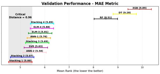
Figure 10.
Model validation performances for the Nemenyi test considering the metric.
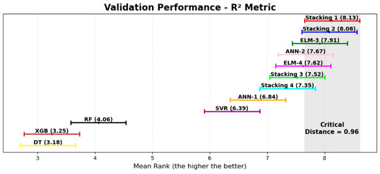
Figure 11.
Model validation performances for the Nemenyi test considering the metric.
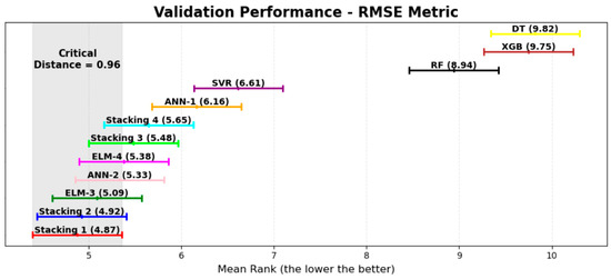
Figure 12.
Model validation performances for the Nemenyi test considering the metric.
The results indicate that although the stacking models did not surpass individual neural networks in testing, the Nemenyi test on the validation dataset suggests that Stacking 1 and Stacking 2 achieved the highest mean rankings across all metrics, followed closely by Stacking 3 and Stacking 4. However, since the critical distance calculated for the test was , and multiple models ranked within this range, no statistically significant differences were observed among the stacking models or between most neural networks. The GA-ANN-2 (50), AGA-ELM-3 (20), and GA-ELM-4 (50) models fell within the critical distance for all metrics, while AGA-ANN-1 (20) and AGA-SVR (20) were also within this range for .
In contrast, the tree-based models exhibited consistently lower predictive performance when compared to other approaches. The Nemenyi test results reinforce that these models behave similarly, with less capacity to predict accurately for the studied dataset. The findings confirm that while the stacking models performed well, they did not provide a statistically significant advantage over the best individual neural networks.
3.5. Main Findings of This Study
Based on the results obtained throughout the hyperparameter tuning, training, testing, and validation stages, as well as the nonparametric statistical tests, this study successfully met its primary objectives. The key findings can be summarized as follows:
- Despite the relatively small dataset used for predicting dilution () in underground mines and the low correlation of some independent variables with , the proposed methodology enabled the development of multiple machine learning models capable of accurately predicting from the given dataset.
- The application of genetic algorithms (GA and AGA) with varying population sizes strengthened the hyperparameter tuning process, leading to models with improved generalization capabilities for unseen data.
- Incorporating machine learning models based on different paradigms and strategies provided a robust analytical framework, facilitating the assessment of the strengths and weaknesses of each model within the proposed scope.
- The performance limitations observed in certain models within this study should not be generalized, as machine learning models are highly sensitive to data characteristics and may perform differently when applied to other datasets or problem domains.
- Implementing a cross-validation procedure with 10 folds and 30 repetitions allowed for a more comprehensive analysis, ensuring that even a small dataset could be evaluated rigorously. The statistical tests confirmed the superiority of certain models, while refuting the existence of significant performance differences between others.
- The methodology emphasized the importance of a well-structured validation phase. A simple division into training and testing datasets may bias the results in favor of a specific model configuration, which, when exposed to different data partitions, may fail to maintain its performance.
- The study demonstrated that stacking metamodels built from distinct base models can be equally or even more effective than the use of individual models, as confirmed by the Nemenyi test results.
- Although AGA-ANN-1 (20) was identified as the best-performing model during the testing phase, it was not among the top models in two out of three Nemenyi test evaluations. This finding underscores the risk of relying solely on a single test dataset, particularly when dealing with small datasets, as it may lead to anomalies and models that do not consistently deliver optimal results.
3.6. Limitations of This Study
Despite the statistically robust methodology adopted and the satisfactory predictive performance achieved, this study is subject to several limitations that should be acknowledged:
- The representativeness of the dataset is intrinsically linked to the geological and operational characteristics of the mines from which the data were collected. Therefore, the models developed herein may not generalize effectively to mines with substantially different conditions.
- Potential sampling biases or errors in data collection could have introduced distortions in the training process, leading to models that do not adequately capture the underlying relationships within the studied context.
- The relatively small dataset size (120 samples) imposes limitations on the models’ ability to generalize. In particular, the identification of more subtle patterns may be hindered, and statistical fluctuations across different data partitions may be exacerbated.
- Decisions regarding data transformation strategies, train–test segmentation, choice of machine learning algorithms, and hyperparameter optimization configurations—although carefully considered—may not represent the optimal combination. These choices can impact model performance and generalization capacity.
- The genetic algorithms employed for hyperparameter tuning, while effective in navigating complex search spaces, do not guarantee convergence to global optima. As a result, superior configurations may remain unexplored.
- The performance of the stacking models is inherently constrained by the predictive capabilities of the constituent base models. Consequently, under different scenarios or datasets, the ensemble approach may not yield improved robustness or accuracy.
4. Conclusions
This study proposed a practical framework for predicting dilution in underground mining operations by integrating machine learning (ML) models with genetic algorithms (GAs). Grounded in a statistically rigorous methodology, the proposed approach encompassed hyperparameter tuning, model training, testing, and validation, thereby enabling a comprehensive evaluation of predictive performance based on the dataset employed. Among the primary contributions of this work is the novel use of stacking models—constructed from individually optimized ML-based models—to address this task for the first time. The methodological pipeline, which includes stratified sampling to preserve the original distribution of the target variable, a repeated k-fold strategy to enhance cross-validation robustness, a 10-fold cross-validation procedure with 30 repetitions for reliable performance assessment, and the application of nonparametric statistical tests, constitutes a statistically sound framework that can support future research in the field.
Despite the relatively limited dataset—comprising only 120 samples—and the computational constraints imposed by the use of a standard personal laptop, several ML-based models demonstrated remarkable predictive capabilities. Among the approaches evaluated, which included support vector machines (SVMs), tree-based models, and artificial neural networks (ANNs), the neural network-based models consistently outperformed the others in predicting dilution. The AGA-ANN-1 model with a population size of 20 individuals achieved , , and values of 0.2986, 0.8457, and 0.3928 on the training dataset, and 0.1882, 0.9508, and 0.2283 on the testing dataset, respectively. Comparable performance was observed for the extreme learning machine (ELM) models, a variant of neural networks, with both AGA-ELM-3 (20) and GA-ELM-4 (50) yielding , , and values of 0.1940, 0.9544, and 0.2197, respectively, on the testing set. Furthermore, to assess the potential benefits of model ensembling, four stacking models were constructed. The most effective configuration—Stacking 3—combined the AGA-ANN-1 (20), AGA-ELM-3 (20), GA-ANN-2 (50), and AGA-SVR (20) models, achieving testing set metrics of 0.2177 for , 0.9246 for , and 0.2826 for .
Additionally, an analysis of the validation metrics revealed that all neural network-based models, the SVR model, and all stacking configurations exhibited comparable performance. Although the Stacking 1 model—comprising AGA-ANN-1 (20) and AGA-ELM-3 (20)—achieved the best average validation results, with mean , , and values of 0.3476 ± 0.0952, 0.7454 ± 0.1570, and 0.4483 ± 0.1230, respectively, these metrics alone were not sufficient to conclusively establish the superiority of the stacking models over the individual neural network-based models. However, the application of nonparametric statistical tests confirmed that all stacking models were at least as robust as and in some cases, statistically superior to, the individual models examined.
Future research could explore the predictive capabilities of additional ML models, such as AdaBoost, gradient boosting machines (GBM), and radial basis networks (RBN) [66,67]. Further improvements in hyperparameter optimization could be achieved by integrating alternative metaheuristics, including cuckoo search optimization (CSO) and ant colony optimization (ACO) [85,86]. Given the small size of the dataset used in this study, collecting a larger dataset would be crucial for improving model reliability and reducing variability across different data splits. In this regard, data augmentation techniques, such as generative adversarial networks (GANs) and variational autoencoders (VAEs) [87], could be explored. However, their potential benefits should be carefully evaluated, as there is no definitive guarantee that synthetic data generation will enhance model performance. Finally, considering that dilution and stope stability in underground mining operations are intrinsically linked to stope exposure time, addressing these tasks through a time series perspective [65] may enable practitioners to anticipate stope behavior over time and implement timely interventions to enhance operational safety at the work fronts.
Author Contributions
Conceptualization, J.L.V.M.; methodology, J.L.V.M., T.S.G.F. and R.M.A.S.; software, J.L.V.M. and T.S.G.F.; validation, J.L.V.M., T.S.G.F. and H.J.; formal analysis, J.L.V.M., T.S.G.F. and R.M.A.S.; investigation, J.L.V.M., T.S.G.F. and R.M.A.S.; resources, J.L.V.M. and T.S.G.F.; data curation, M.P.L. and J.L.V.M.; writing—original draft preparation, J.L.V.M.; writing—review and editing, J.L.V.M., T.S.G.F., R.M.A.S. and H.J.; visualization, J.L.V.M. and T.S.G.F.; supervision, R.M.A.S.; project administration, J.L.V.M. All authors have read and agreed to the published version of the manuscript.
Funding
The APC was partially funded by the Computer Center from the Universidade Federal de Pernambuco.
Institutional Review Board Statement
Not applicable.
Informed Consent Statement
Not applicable.
Data Availability Statement
The data used in this study were published by Zhao and Niu [51] and are available at https://www.mdpi.com/2071-1050/12/4/1550 (accessed on 23 April 2025).
Conflicts of Interest
The authors declare no conflicts of interest.
Appendix A
Appendix A provides a reference list of the abbreviations used throughout this paper.
Table A1.
List of abbreviations used in this study.
Table A1.
List of abbreviations used in this study.
| List of Abbreviations | |
|---|---|
| ABC: artificial bee colony | LDA: linear discriminant analysis |
| ACO: ant colony optimization | LightGBM: light gradient boosting machine |
| AGA: adaptive genetic algorithm | MABAC: multi-attributive approximation area comparison |
| AI: artificial intelligence | : mean absolute error |
| ALO: ant lion optimizer | ML: machine learning |
| ANFIS: adaptive neuro-fuzzy inference system | MLRA: multi linear regression analysis |
| ANN: artificial neural network | MNRA: multi nonlinear regression analysis |
| AUC: area under the curve | MR: memory replay |
| BD: mean borehole deviation | MSE: mean-square error |
| BO: Bayesian optimization | N′: modified stability number |
| CART: classification and regression tree | ORF: overbreak resistance factor |
| CatBoost: categorical boosting | PCA: principal component analysis |
| CGA: conjugate gradient algorithm | PF: powder factor |
| CNFS: concurrent neuro-fuzzy system | PSO: particle swarm optimization |
| CSO: cuckoo search optimization | Q′: modified rock mass quality index |
| DF21: Deep Forest 21 | R: correlation coefficient |
| DT: decision tree | : coefficient of determination |
| ELM: extreme learning machine | RBN: radial basis network |
| : equivalent linear overbreak slough | RF: random forest |
| EM: expectation maximization | RMR: rock mass rating |
| EWC: elastic weight consolidation | : root-mean-square error |
| FA: firefly algorithm | RNN: recurrent neural network |
| FIS: fuzzy inference system | RQD: rock quality designation |
| FMF: fuzzy membership function | SRF: stress reduction factor |
| GA: genetic algorithm | SSA: sparrow search algorithm |
| GAN: generative adversarial network | SSE: stepwise selection and elimination |
| GBDT: gradient boosting decision tree | SUDI: stope unplanned dilution index |
| GBM: gradient boosting machine | SVM: support vector machine |
| gcForest: grained cascade forest | SVR: support vector regression |
| GPC: Gaussian process classification | TOPSIS: technique for order of preference by similarity to ideal solution |
| GRNN: generalized regression neural network | TSA: tunicate swarm algorithm |
| GSI: geological strength index | UF: undercutting factor |
| GWO: grey wolf optimizer | VAE: variational autoencoder |
| HR: hydraulic radius | WOA: whale optimization algorithm |
| K: average horizontal to vertical stress ratio | WNN: wavelet neural network |
| KNN: k-nearest neighbors | XGB: extreme gradient boosting |
Appendix B
Appendix B provides the optimized hyperparameter values for the best-performing machine learning models, as determined by the selection criteria outlined in the methodology.
Table A2.
Hyperparameters of the best DT model according to the adopted criterion, GA-DT (20).
Table A2.
Hyperparameters of the best DT model according to the adopted criterion, GA-DT (20).
| DT Hyperparameters | Optimized Values |
|---|---|
| Min weight fraction leaf | 0.0412 |
| Max depth | 61 |
| Min samples leaf | 3 |
| Min samples split | 4 |
| Criterion | absolute_error |
Table A3.
Hyperparameters of the best RF model according to the adopted criterion, AGA-RF (80).
Table A3.
Hyperparameters of the best RF model according to the adopted criterion, AGA-RF (80).
| RF Hyperparameters | Optimized Values |
|---|---|
| Ccp alpha | 0.0100 |
| N estimators | 537 |
| Max depth | 5 |
| Min samples leaf | 1 |
| Min samples split | 2 |
| Criterion | absolute_error |
Table A4.
Hyperparameters of the best XGB model according to the adopted criterion, GA-XGB (20).
Table A4.
Hyperparameters of the best XGB model according to the adopted criterion, GA-XGB (20).
| XGB Hyperparameters | Optimized Values |
|---|---|
| N estimators | 833 |
| Max depth | 27 |
| Eta | 0.0165 |
| Subsample | 0.1529 |
| Colsample by tree | 1.0000 |
Table A5.
Hyperparameters of the best SVR model according to the adopted criterion, AGA-SVR (20).
Table A5.
Hyperparameters of the best SVR model according to the adopted criterion, AGA-SVR (20).
| SVR Hyperparameters | Optimized Values |
|---|---|
| Kernel | rbf |
| C | 10.0000 |
| Gamma | 0.0500 |
Table A6.
Hyperparameters of the best ANN-1 model according to the adopted criterion, AGA-ANN-1 (20).
Table A6.
Hyperparameters of the best ANN-1 model according to the adopted criterion, AGA-ANN-1 (20).
| ANN-1 Hyperparameters | Optimized Values |
|---|---|
| Number of layers | 1 |
| Layer sizes (nodes per layer) | 15 |
| Learning rate | 0.0484 |
| Dropout rate | 0.0902 |
| Weight decay | 0.0010 |
| Epochs | 30 |
| Activation | relu |
| Solver | adam |
Table A7.
Hyperparameters of the best ANN-2 model according to the adopted criterion, GA-ANN-2 (50).
Table A7.
Hyperparameters of the best ANN-2 model according to the adopted criterion, GA-ANN-2 (50).
| ANN-2 Hyperparameters | Optimized Values |
|---|---|
| Number of layers | 2 |
| Layer sizes (nodes per layer) | 16, 18 |
| Learning rate | 0.0227 |
| Dropout rate | 0.0157 |
| Weight decay | 0.0041 |
| Epochs | 45 |
| Activation | leaky_relu |
| Solver | adam |
Table A8.
Hyperparameters of the best ELM-3 model according to the adopted criterion, AGA-ELM-3 (20).
Table A8.
Hyperparameters of the best ELM-3 model according to the adopted criterion, AGA-ELM-3 (20).
| ELM-3 Hyperparameters | Optimized Values |
|---|---|
| Number of layers | 3 |
| Layer sizes (nodes per layer) | 4, 2, 2 |
| Alpha | 0.1000 |
| Density | 0.1529 |
| Include original features | False, True, True |
| Ufunc | tanh, lin, tanh |
| Pairwise metric | hamming, hamming, Euclidean |
Table A9.
Hyperparameters of the best ELM-4 model according to the adopted criterion, GA-ELM-4 (50).
Table A9.
Hyperparameters of the best ELM-4 model according to the adopted criterion, GA-ELM-4 (50).
| ELM-4 Hyperparameters | Optimized Values |
|---|---|
| Number of layers | 4 |
| Layer sizes (nodes per layer) | 17, 6, 2, 11 |
| Alpha | 0.0961 |
| Density | 0.9177 |
| Include original features | True, True, True, True |
| Ufunc | tanh, lin, tanh, None |
| Pairwise metric | hamming, hamming, Euclidean, hamming |
References
- Brady, B.H.G.; Brown, E.T. Rock Mechanics for Underground Mining, 3rd ed.; Springer: Dordrecht, The Netherlands, 2004. [Google Scholar]
- Pontow, S.J. Evaluation of Methods for Stope Design in Mining and Potential of Improvement by Pre-Investigations. Master’s Thesis, Aalto University, Espoo, Finland, 2019. [Google Scholar]
- Cadenillas, C.T. Prediction of Unplanned Dilution in Underground Mines Through Machine Learning Techniques. Master’s Thesis, McGill University, Montreal, QC, Canada, 2023. [Google Scholar]
- Wang, J. Influence of Stress, Undercutting, Blasting and Time on Open Stope Stability and Dilution. Ph.D. Thesis, University of Saskatchewan, Saskatoon, SK, Canada, 2004. [Google Scholar]
- Potvin, Y. Empirical Open Stope Design in Canada. Ph.D. Thesis, University of British Columbia, Vancouver, BC, Canada, 1988. [Google Scholar]
- Clark, L.M. Minimizing Dilution in Open Stope Mining with a Focus on Stope Design and Narrow Vein Longhole Blasting. Master’s Thesis, University of British Columbia, Vancouver, BC, Canada, 1998. [Google Scholar]
- Lima, M.P.; Guimarães, L.J.N.; Gomes, I.F. Numerical modeling of the underground mining stope stability considering time-dependent deformations via finite element method. REM Int. Eng. J. 2024, 77, e230080. [Google Scholar] [CrossRef]
- Panji, M.; Koohsari, H.; Adampira, M.; Alielahi, H.; Marnani, J.A. Stability analysis of shallow tunnels subjected to eccentric loads by a boundary element method. J. Rock Mech. Geotech. Eng. 2016, 8, 480–488. [Google Scholar] [CrossRef]
- Deere, D.U. Technical description of rock cores for engineering purposes. Rock Mech. Rock Eng. 1964, 1, 17–22. [Google Scholar]
- ISRM Commission. Suggested methods for the quantitative description of discontinuities in rock masses. Int. J. Rock Mech. Min. Sci. Geomech. Abstr. 1978, 15, 319–368. [Google Scholar]
- Hoek, E.; Brown, E.T. Underground Excavations in Rock; Institution of Mining and Metallurgy: London, UK, 1980. [Google Scholar]
- Bieniawski, Z.T. Engineering classification of jointed rock masses. Trans. S. Afr. Inst. Civ. Eng. 1973, 15, 335–344. [Google Scholar]
- Bieniawski, Z.T. Rock mass classifications in rock engineering. In Proceedings of the Exploration for Rock Engineering, Johannesburg, South Africa, 1–5 November 1976. [Google Scholar]
- Bieniawski, Z.T. Engineering Rock Mass Classifications: A Complete Manual for Engineers and Geologists in Mining, Civil, and Petroleum Engineering; John Wiley & Sons: Hoboken, NJ, USA, 1989. [Google Scholar]
- Barton, N.R.; Lien, R.; Lunde, J. Engineering classification of rock masses for the design of tunnel support. Rock Mech. 1974, 6, 189–239. [Google Scholar] [CrossRef]
- Hoek, E. Strength of rock and rock masses. ISRM News J. 1994, 2, 4–16. [Google Scholar]
- Hoek, E.; Kaiser, P.K.; Bawden, W.F. Support of Underground Excavations in Hard Rock; A. A. Balkema: Rotterdam, The Netherlands, 1995. [Google Scholar]
- Hoek, E.; Carranza, C.; Corkum, B. Hoek-Brown failure criterion—2002 Edition. In Proceedings of the NARMS-TAC 2002, Toronto, ON, Canada, 7–10 July 2002. [Google Scholar]
- Grimstad, E.; Barton, N.R. Updating of the Q-system for NMT. In Proceedings of the International Symposium on Sprayed Concrete, Fagernes, Norway, 17–21 October 1993. [Google Scholar]
- Hoek, E.; Brown, E.T. The Hoek–Brown failure criterion: A 1988 update. In Proceedings of the 15th Canadian Rock Mechanics Symposium, Toronto, Canada, 3–4 October 1988. [Google Scholar]
- Diederichs, M.S.; Kaiser, P.K. Tensile strength and abutment relaxation as failure control mechanisms in underground excavations. Int. J. Rock Mech. Min. Sci. 1999, 36, 69–96. [Google Scholar] [CrossRef]
- Adoko, A.C.; Saadaari, F.; Mireku-Gyimah, D.; Imashev, A. A Feasibility Study on The Implementation of Neural Network Classifiers for Open Stope Design. Geotech. Geol. Eng. 2022, 40, 677–696. [Google Scholar] [CrossRef]
- Henning, J.G.; Mitri, H.S. Numerical modelling of ore dilution in blasthole stoping. Int. J. Rock Mech. Min. Sci. 2007, 44, 692–703. [Google Scholar] [CrossRef]
- Heidarzadeh, S.; Saeidi, A.; Rouleau, A. Evaluation of the effect of geometrical parameters on stope probability of failure in the open stoping method using numerical modeling. Int. J. Min. Sci. Technol. 2019, 29, 399–408. [Google Scholar] [CrossRef]
- Cepuritis, P.M.; Villaescusa, E.; Beck, D.A.; Varden, R. Back Analysis of Over-Break in a Longhole Open Stope Operation Using Non-Linear Elasto-Plastic Numerical Modelling. In Proceedings of the 44th U.S. Rock Mechanics Symposium and 5th U.S.-Canada Rock Mechanics Symposium, Salt Lake City, UT, USA, 27–30 June 2010. [Google Scholar]
- Cordova, D.P.; Zingano, A.C.; Gonçalves, I.G. Unplanned dilution back analysis in an underground mine using numerical models. REM Int. Eng. J. 2022, 75, 379–388. [Google Scholar] [CrossRef]
- Mathews, K.; Hoek, E.; Wyllie, D.; Stewart, S. Prediction of Stable Excavation Spans at Depths Below 1000 m in Hard Rock Mines; CANMET Report, DSS Serial No OSQ80–00081; Canada Centre for Mineral and Energy Technology: Ottawa, ON, Canada, 1981. [Google Scholar]
- Clark, L.M.; Pakalnis, R.C. An empirical design approach for estimating unplanned dilution from open stope hangingwalls and footwalls. In Proceedings of the CIM’97: 99th Annual General Meeting, Vancouver, BC, Canada, 26 April–1 May 1997; Canadian Institute of Mining, Metallurgy and Petroleum: Vancouver, BC, Canada, 1997. [Google Scholar]
- Suorineni, F.T.; Kaiser, P.K.; Tannant, D.D. Likelihood statistic for interpretation of the stability graph for open stope design. Int. J. Rock Mech. Min. Sci. 2001, 38, 735–744. [Google Scholar] [CrossRef]
- Yuan, J.; Zhou, C.; Zhang, D. Physical model test and numerical simulation study of deformation mechanism of wall rock on open pit to underground mining. Int. J. Eng. 2014, 27, 1795–1802. [Google Scholar]
- Bazaluk, O.; Petlovanyi, M.; Zubko, S.; Lozynskyi, V.; Sai, K. Instability assessment of hanging wall rocks during underground mining of iron ores. Minerals 2021, 11, 858. [Google Scholar] [CrossRef]
- Germain, P.; Hadjigeorgiou, J. Influence of stope geometry and blasting pattern on recorded overbreak. Int. J. Rock Mech. Min. Sci. 1997, 34, 115.e1–115.e12. [Google Scholar] [CrossRef]
- Jang, H.; Topal, E. Optimizing overbreak prediction based on geological parameters comparing multiple regression analysis and artificial neural network. Tunn. Undergr. Space Technol. 2013, 38, 161–169. [Google Scholar] [CrossRef]
- Sun, S.; Liu, J.; Wei, J. Predictions of overbreak blocks in tunnels based on the wavelet neural network method and the geological statistics theory. Math. Probl. Eng. 2013, 2013, 706491. [Google Scholar]
- Jang, H. Unplanned Dilution and Ore-Loss Optimisation in Underground Mines via Cooperative Neuro-Fuzzy Network. Ph.D. Thesis, Curtin University, Perth, WA, Australia, 2014. [Google Scholar]
- Jang, H.; Topal, E.; Kawamura, Y. Unplanned dilution and ore loss prediction in longhole stoping mines via multiple regression and artificial neural network analyses. J. South. Afr. Inst. Min. Metall. 2015, 115, 449–456. [Google Scholar] [CrossRef]
- Jang, H.; Topal, E.; Kawamura, Y. Decision support system of unplanned dilution and ore-loss in underground stoping operations using a neuro-fuzzy system. Appl. Soft Comput. 2015, 32, 1–12. [Google Scholar] [CrossRef]
- Mohammadi, M.; Hossaini, M.F.; Mirzapour, B.; Hajiantilaki, N. Use of fuzzy set theory for minimizing overbreak in underground blasting operations—A case study of Alborz Tunnel, Iran. Int. J. Min. Sci. Technol. 2015, 25, 439–445. [Google Scholar] [CrossRef]
- Mohseni, M.; Ataei, M.; Khaloo Kakaie, R. A new classification system for evaluation and prediction of unplanned dilution in cut-and-fill stoping method. J. Min. Environ. 2018, 9, 873–892. [Google Scholar]
- Mottahedi, A.; Sereshki, F.; Ataei, M. Development of overbreak prediction models in drill and blast tunneling using soft computing methods. Eng. Comput. 2018, 34, 45–58. [Google Scholar] [CrossRef]
- Mottahedi, A.; Sereshki, F.; Ataei, M. Overbreak prediction in underground excavations using hybrid ANFIS-PSO model. Tunn. Undergr. Space Technol. 2018, 80, 1–9. [Google Scholar] [CrossRef]
- Qi, C.; Fourie, A.; Du, X.; Tang, X. Prediction of open stope hangingwall stability using random forests. Nat. Hazards 2018, 92, 1179–1197. [Google Scholar] [CrossRef]
- Capes, G.W. Open Stope Hangingwall Design Based on General and Detailed Data Collection in Unfavourable Hangingwall Conditions. Ph.D. Thesis, University of Saskatchewan, Saskatoon, SK, Canada, 2009. [Google Scholar]
- Qi, C.; Fourie, A.; Ma, G.; Tang, X.; Du, X. Comparative study of hybrid artificial intelligence approaches for predicting hangingwall stability. J. Comput. Civ. Eng. 2018, 32, 04017086. [Google Scholar] [CrossRef]
- Qi, C.; Fourie, A.; Ma, G.; Tang, X. A hybrid method for improved stability prediction in construction projects: A case study of stope hangingwall stability. Appl. Soft Comput. 2018, 71, 649–658. [Google Scholar] [CrossRef]
- Jang, H.; Taheri, S.; Topal, E.; Kawamura, Y. Illumination of contributing parameters of uneven break in narrow vein mine. In Proceedings of the 28th International Symposium on Mine Planning and Equipment Selection—MPES 2019, Perth, WA, Australia, 2–4 December 2019. [Google Scholar]
- Jang, H.; Kawamura, Y.; Shinji, U. An empirical approach of overbreak resistance factor for tunnel blasting. Tunn. Undergr. Space Technol. 2019, 92, 103060. [Google Scholar] [CrossRef]
- Koopialipoor, M.; Armaghani, D.J.; Haghighi, M.; Ghaleini, E.N. A neuro-genetic predictive model to approximate overbreak induced by drilling and blasting operation in tunnels. Bull. Eng. Geol. Environ. 2019, 78, 981–990. [Google Scholar] [CrossRef]
- Koopialipoor, M.; Ghaleini, E.N.; Tootoonchi, H.; Armaghani, D.J.; Haghighi, M.; Hedayat, A. Developing a new intelligent technique to predict overbreak in tunnels using an artificial bee colony-based ANN. Environ. Earth Sci. 2019, 78, 8163. [Google Scholar] [CrossRef]
- Koopialipoor, M.; Ghaleini, E.N.; Haghighi, M.; Kanagarajan, S.; Maarefvand, P.; Mohamad, E.T. Overbreak prediction and optimization in tunnel using neural network and bee colony techniques. Eng. Comput. 2019, 35, 1191–1202. [Google Scholar] [CrossRef]
- Zhao, X.; Niu, J. Method of predicting ore dilution based on a neural network and its application. Sustainability 2020, 12, 1550. [Google Scholar] [CrossRef]
- Bazarbay, B.; Adoko, A.C. A Comparison of Prediction and Classification Models of Unplanned Stope Dilution in Open Stope Design. In Proceedings of the 55th U.S. Rock Mechanics/Geomechanics Symposium, Houston, TX, USA, 18–25 June 2021. [Google Scholar]
- Bazarbay, B.; Adoko, A.C. Development of a knowledge-based system for assessing unplanned dilution in open stopes. IOP Conf. Ser. Earth Environ. Sci. 2021, 861, 062086. [Google Scholar] [CrossRef]
- Mohseni, M.; Ataei, M.; Kakaie, R. Dilution risk ranking in underground metal mines using Multi Attributive Approximation Area Comparison. J. Min. Environ. 2020, 11, 977–989. [Google Scholar]
- Korigov, S.; Adoko, A.C.; Sengani, F. Unplanned dilution prediction in open stope mining: Developing new design charts using Artificial Neural Network classifier. J. Sustain. Min. 2022, 21, 157–168. [Google Scholar] [CrossRef]
- Jorquera, M.; Korzeniowski, W.; Skrzypkowski, K. Prediction of dilution in sublevel stoping through machine learning algorithms. IOP Conf. Ser. Earth Environ. Sci. 2023, 1189, 012008. [Google Scholar] [CrossRef]
- He, B.; Armaghani, D.J.; Lai, S.H. Assessment of tunnel blasting-induced overbreak: A novel metaheuristic-based random forest approach. Tunn. Undergr. Space Technol. 2023, 133, 104979. [Google Scholar] [CrossRef]
- Hong, Z.; Tao, M.; Liu, L.; Zhao, M.; Wu, C. An intelligent approach for predicting overbreak in underground blasting operation based on an optimized XGB model. Eng. Appl. Artif. Intell. 2023, 126, 107097. [Google Scholar] [CrossRef]
- Liu, Y.; Li, A.; Zhang, H.; Wang, J.; Li, F.; Chen, R.; Wang, S.; Yao, J. Minimization of overbreak in different tunnel sections through predictive modeling and optimization of blasting parameters. Front. Ecol. Evol. 2023, 11, 1255384. [Google Scholar] [CrossRef]
- Zhang, W. Research on Blasthole Image Recognition Algorithms and Optimization of Smooth Blasting Parameters of Rock Tunnel. Ph.D. Thesis, Shandong University, Jinan, China, 2020. [Google Scholar]
- Liu, Y.; Li, A.; Wang, S.; Yuan, J.; Zhang, X. A feature importance-based intelligent method for controlling overbreak in drill-and-blast tunnels via integration with rock mass quality. Alex. Eng. J. 2024, 108, 1011–1031. [Google Scholar] [CrossRef]
- Chimunhu, P.; Faradonbeh, R.S.; Topal, E.; Asad, M.W.A.; Ajak, A.D. Development of novel hybrid intelligent predictive models for dilution prediction in underground sub-level mining. Min. Metall. Explor. 2024, 41, 2079–2098. [Google Scholar] [CrossRef]
- Li, C.; Dias, D.; Zhou, J.; Tao, M. Applying a novel hybrid ALO-BPNN model to predict overbreak and underbreak area in underground space. In Applications of Artificial Intelligence in Mining and Geotechnical Engineering; Nguyen, H., Bui, X.-N., Topal, E., Zhou, J., Choi, Y., Zhang, W., Eds.; Elsevier: Amsterdam, The Netherlands, 2024; pp. 325–342. [Google Scholar]
- He, B.; Li, J.; Armaghani, D.J.; Hashim, H.; He, X.; Pradhan, B.; Sheng, D. The deep continual learning framework for prediction of blast-induced overbreak in tunnel construction. Expert Syst. Appl. 2025, 264, 125909. [Google Scholar] [CrossRef]
- Cieślik, K.; Milczarek, W. Application of machine learning in forecasting the impact of mining deformation: A case study of underground copper mines in Poland. Remote Sens. 2022, 14, 4755. [Google Scholar] [CrossRef]
- Raschka, S.; Liu, Y.; Mirjalili, V. Machine Learning with PyTorch and Scikit-Learn: Develop Machine Learning and Deep Learning Models with Python; Packt Publishing Ltd.: Birmingham, UK, 2022. [Google Scholar]
- Bataineh, M.; Marler, T. Neural network for regression problems with reduced training sets. Neural Netw. 2017, 95, 1–9. [Google Scholar] [CrossRef] [PubMed]
- Wolpert, D.H. Stacked generalization. Neural Netw. 1992, 5, 241–259. [Google Scholar] [CrossRef]
- Demsar, J. Statistical comparisons of classifiers over multiple data sets. J. Mach. Learn. Res. 2006, 7, 1–30. [Google Scholar]
- Mcculloch, W.S.; Pitts, W. A logical calculus of the ideas immanent in nervous activity. Bull. Math. Biophys. 1943, 5, 115–133. [Google Scholar] [CrossRef]
- Rosenblatt, F. The perceptron: A probabilistic model for information storage and organization in the brain. Psychol. Rev. 1958, 65, 386–408. [Google Scholar] [CrossRef]
- Rumelhart, D.E.; Hinton, G.E.; Williams, R.J. Learning representations by back-propagating errors. Nature 1986, 323, 533–536. [Google Scholar] [CrossRef]
- Huang, G.-B.; Zhu, Q.-Y.; Siew, C.-K. Extreme learning machine: Theory and applications. Neurocomputing 2006, 70, 489–501. [Google Scholar] [CrossRef]
- Vapnik, V.N.; Chervonenkis, A.Y. On a class of pattern-recognition learning algorithms. Automation and Remote Control 1964, 25, 838–845. [Google Scholar]
- Vapnik, V.; Golowich, S.E.; Smola, A. Support vector method for function approximation, regression estimation and signal processing. In Proceedings of the 9th International Conference on Neural Information Processing Systems, Denver, CO, USA, 2–5 December 1996. [Google Scholar]
- Morgan, J.N.; Sonquist, J.A. Problems in the analysis of survey data, and a proposal. J. Am. Stat. Assoc. 1963, 58, 415–434. [Google Scholar] [CrossRef]
- Breiman, L. Random forests. Mach. Learn. 2001, 45, 5–32. [Google Scholar] [CrossRef]
- Chen, T.; Guestrin, C. XGB: A scalable tree boosting system. In Proceedings of the KDD’16: The 22nd ACM SIGKDD International Conference on Knowledge Discovery and Data Mining, San Francisco, CA, USA, 13–17 August 2016. [Google Scholar]
- Yasser, A.A.; Awwad, E.M.; Al-Razgan, M.; Maarouf, A. Hyperparameter search for machine learning algorithms for optimizing the computational complexity. Processes 2023, 11, 349. [Google Scholar] [CrossRef]
- Ilemobayo, J.A.; Durodola, O.; Alade, O.; Awotunde, O.J.; Olanrewaju, A.T.; Falana, O.; Ogungbire, A.; Osinuga, A.; Ogunbiyi, D.; Ifeanyi, A.; et al. Hyperparameter tuning in machine learning: A comprehensive review. J. Eng. Res. Rep. 2024, 26, 388–395. [Google Scholar] [CrossRef]
- Holland, J.H. Adaptation in Natural and Artificial Systems: An Introductory Analysis with Applications to Biology, Control, and Artificial Intelligence; University of Michigan Press: Ann Harbor, MI, USA, 1975. [Google Scholar]
- Friedman, M. A comparison of alternative tests of significance for the problem of m rankings. Ann. Math. Stat. 1940, 11, 86–92. [Google Scholar] [CrossRef]
- Nemenyi, P.B. Distribution-Free Multiple Comparisons. Ph.D. Thesis, Princeton University, Princeton, NJ, USA, 1963. [Google Scholar]
- Yeo, I.K.; Johnson, R.A. A new family of power transformations to improve normality or symmetry. Biometrika 2000, 87, 954–959. [Google Scholar] [CrossRef]
- Dorigo, M. Optimization, Learning and Natural Algorithms. Ph.D. Thesis, Politecnicodi Milano, Milan, Italy, 1992. [Google Scholar]
- Yang, X.-S.; Deb, S. Cuckoo search via Lévy flights. In Proceedings of the World Congress on Nature & Biologically Inspired Computing (NaBIC 2009), Coimbatore, India, 9–11 December 2009. [Google Scholar]
- Kim, D.-K.; Ryu, D.H.; Lee, Y.; Choi, D.-H. Generative models for tabular data: A review. J. Mech. Sci. Technol. 2024, 38, 4989–5005. [Google Scholar] [CrossRef]
Disclaimer/Publisher’s Note: The statements, opinions and data contained in all publications are solely those of the individual author(s) and contributor(s) and not of MDPI and/or the editor(s). MDPI and/or the editor(s) disclaim responsibility for any injury to people or property resulting from any ideas, methods, instructions or products referred to in the content. |
© 2025 by the authors. Licensee MDPI, Basel, Switzerland. This article is an open access article distributed under the terms and conditions of the Creative Commons Attribution (CC BY) license (https://creativecommons.org/licenses/by/4.0/).