Boosting Model Interpretability for Transparent ML in TBM Tunneling

Abstract

Tunnel boring machines (TBMs) are essential for excavating metro tunnels, reducing disruptions to surrounding rock, and ensuring efficient progress. This study examines how machine learning (ML) models can predict key tunneling outcomes, focusing on making these predictions clearer. Specifically, the models aim to predict surface settlements (ground sinking) and the TBM’s penetration rate (PR) during the Athens Metro Line 2 extension to Hellinikon. For surface settlements, four artificial neural networks (ANNs) were developed, achieving an accuracy of over 79%, on average. For the TBM’s PR, both an XGBoost Regressor (XGBR) and ANNs performed consistently well, offering reliable predictions. This study emphasizes model transparency mostly. Using the SHapley Additive exPlanations (SHAP) library, it is possible to explain how models make decisions, highlighting key factors like geological conditions and TBM operating data. With SHAP’s Tree Explainer and Deep Explainer techniques, the study reveals which parameters matter most, making ML models less of a “black box” and more practical for real-world metro tunnel projects. By showing how decisions are made, these tools give decision-makers confidence to rely on ML in complex tunneling operations.

1. Introduction

Research on predicting TBM performance has leveraged various machine learning (ML) approaches, including multiple linear regression [1], ANNs [2], fuzzy logic [3], and deep learning [4], all yielding promising results. Despite tunneling uncertainties, past knowledge has informed models for both specific cases and generalized scenarios [5]. Advanced AI techniques, such as neuro-fuzzy methods [6], particle swarm optimization [7], and hybrid algorithms [8], continue to enhance accuracy and address limitations.

Recent advances include the XGBoost algorithm [9], renowned for its regression and classification capabilities. Fine-tuning XGBoost with Bayesian optimization has achieved impressive predictions of the TBM advance rate (AR) [10]. To meet the demands of real-time analysis during construction, BIM-based simulations and integrated “BIM-to-FEM” planning systems highlight the field’s progress [11].

ML has revolutionized problem-solving across domains by providing predictive insights and improving decision-making. Ensemble methods, which combine multiple models for greater accuracy, exemplify this transformation [12]. The SHAP library addresses this challenge by explaining each feature’s contribution to predictions, enhancing trust and usability. Its versatility and solid theoretical foundation make it a valuable tool across fields. In tunneling, SHAP has helped evaluate factors influencing settlement outcomes in shield tunneling [13], control shield attitude [14], and predicting fire-induced spalling in concrete tunnel linings [15]. Additionally, SHAP has clarified how geological conditions impact TBM penetration rates [15,16,17]. While some movement reduces stresses and costs, excessive deformation risks destructive surface settlements.

Predicting settlements is essential to minimizing deformations and preventing soil volume loss. These include immediate settlements, those from tunnel lining deformation, and long-term effects like primary consolidation and secondary creep [18]. Understanding these movements is critical for evaluating TBM performance and planning successful projects.

TBM efficiency also depends on factors such as rock type, operational parameters, and site conditions. The accurate prediction of TBM utilization rates is key to developing effective tunneling plans, enabling proactive measures to enhance efficiency and progress. The TBM utilization percentage directly influences excavation rates and project costs (Farrokh, 2012). The relationship between the rate of penetration (ROP), AR, and utilization (U) is captured in Equation (1).

$$AR=ROP\times U\times T$$

(1)

Increased utilization significantly boosts excavation rates. Even with a high ROP, progress remains slow if TBM usage is inefficient. With typical utilization ranging from less than 10% to around 50%, optimizing machine usage is crucial to ensuring efficient excavation and preventing delays (Figure 1). By managing geotechnical factors and operational parameters, predictive models using ML techniques and SHAP methodology can greatly enhance tunneling project success.

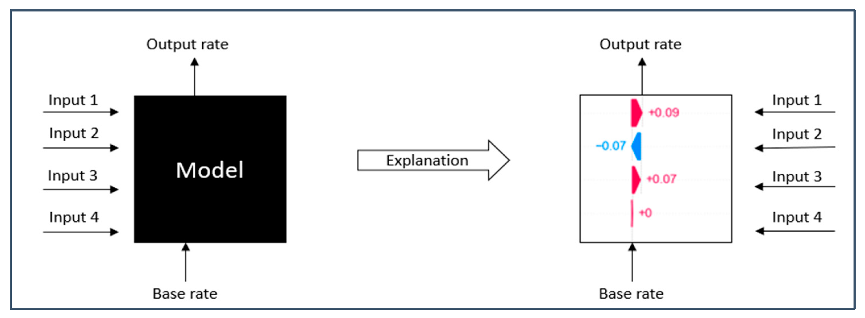
2. Interpretability with SHapley Additive exPlanations (SHAP)

SHAP is a game theory-based method for explaining machine learning model outputs [19]. Shapley values from cooperative game theory fairly distribute credit among features, providing local explanations of a model’s predictions [20,21].

To illustrate, consider a team working toward a combined value (the coalition value). The challenge is determining each member’s contribution, especially when interactions make the whole greater than the sum of its parts. Shapley values address this by comparing the value of coalitions with and without a specific member. For instance, to calculate a member’s marginal contribution, all possible coalitions with and without that member are evaluated, ensuring a fair measure of their impact.

In model interpretability, SHAP adapts this concept to analyze how individual features influence predictions. By decomposing contributions, SHAP clarifies each feature’s role in the overall model output. The mathematical formula for Shapley values is provided in Equation (2).

$${\varphi }_i\left(f,x\right)=\sum _{z^{\prime }\subseteq x^{\prime }}{\displaystyle \frac{\left|z^{\prime }\right|!\left(M-\left|z^{\prime }\right|-1\right)!}{M!}}\left[f_x\left(z^{\prime }\right)-f_x\left(z^{\prime }\setminus \mathrm{i}\right)\right]$$

(2)

where the variables are defined as follows:

• φ_i (f,x) is the Shapley value for feature i, f is the black box model, and x is the input datapoint.
• z′ is the subset.
• x′ is the simplified input.
• M is the total number of features and |z′|!(M − |z′| − 1)!/M! is the weighting.
• f_x is the black box model output and [f_x (z′) − f_x (z′∖i)] is the contribution.

To simplify Equation (1), the “Additive” aspect of SHAP is key. In Equation (3), x represents the inputs and f(x) is the model. A simplified input version x′ transforms the feature vector into a binary format, indicating whether each feature is included or excluded. The explanatory model is then represented as g(x′). The key is ensuring the following:

• If x is approximately equal to x′, then g(x′) (Additive Feature Attribution) should be roughly equal to f(x);
• g must conform to the structure where φ₀ represents the null output of the model (average output of the model) and φ₁ denotes the explained effect of feature 1 (indicating how much feature 1 alters the model’s output). This is referred to as attribution.

$$\begin{array}{l}1.\hspace{1em}x=x^{\prime }\Rightarrow f\left(x\right)=g\left(x^{\prime }\right)\\ 2.\hspace{1em}g\left(x^{\prime }\right)={\varphi }_0+{\sum }_{i=1}^N{\varphi }_i{x}_{i }\end{array}$$

(3)

SHAP creates an explanatory model that highlights each feature’s contribution and importance through its phi values. This additive approach relies on three key properties as follows:

• Local accuracy: when the input and simplified input are nearly identical, the explanatory model should match the actual model’s output.

f(x)≈g(x′) if x≈x′

• Missingness: a feature excluded from the model should have zero attribution, indicating no impact on the output.

xi′= 0 => φi = 0

• Consistency: if a feature’s contribution increases in a new model, its attribution in the explanatory model should not decrease.

Different SHAP versions (e.g., low-order SHAP, kernel SHAP, linear SHAP, deep SHAP, tree SHAP) use model-specific assumptions for faster processing. In this paper, Tree Explainer was applied to the XGBoost model and Deep Explainer to the ANN model. Comparing these explainers on the same dataset provides the following key advantages:

• Model understanding: Tree Explainer interprets XGBoost by attributing decisions to individual trees, while Deep Explainer reveals how features influence neural network predictions.
• Complexity comparison: tree models are more interpretable, whereas neural networks are complex; Deep Explainer demystifies the processing in network layers.
• Feature importance: Tree Explainer ranks feature importance for XGBoost, while Deep Explainer highlights impactful features for the ANN.
• Result validation: comparing results across explainers cross-validates findings, boosting confidence in model robustness.
• Task-specific insights: each model excels in different tasks; comparisons highlight their context-specific strengths and weaknesses.
• Decision support: understanding model decision-making is vital for applications like safety and risk assessment, where interpretability is critical.

SHAP plots visually explain how individual features impact model predictions (Figure 2). By breaking down each prediction into feature contributions, they clarify variable influences, making complex models transparent and trustworthy. These plots are essential for explaining models, building trust, and improving confidence in an algorithm’s performance.

3. Machine Learning Model Development

This section analyzes the Athens Metro Line 2 Hellinikon extension project, focusing on advanced machine learning techniques for predicting and analyzing key tunneling operations. Two case studies are presented, namely surface settlements during metro tunnel construction and TBM penetration rate prediction. Using ANNs and XGBoost Regressor (XGBR), these models achieved high predictive accuracy. The real breakthrough, however, was the use of the SHAP library, which provides a practical means of interpreting the decision-making processes of these complex “black box” models.

3.1. Metro Area of Interest

For surface settlement assessment, the study focused on Interval 5 of the metro tunnel extension between Agios Dimitrios and Elliniko, spanning 585 m from the Hymettus intershaft to the Leontos shaft. The TBM penetration rate (PR) analysis covered interstations 6 (Argiroupoli to Hymettus), 5 (Hymettus to Leontos), and 4 (Leontos to Alimos), totaling 1624 m.

In the PR prediction study, geological, geotechnical, and geometry factors were excluded from the machine learning inputs. This tested the hypothesis that operational parameters—like tunnel face pressure—could compensate for geological variations. The aim was to determine whether operational parameters alone could drive efficient tunneling, minimizing the influence of geological factors.

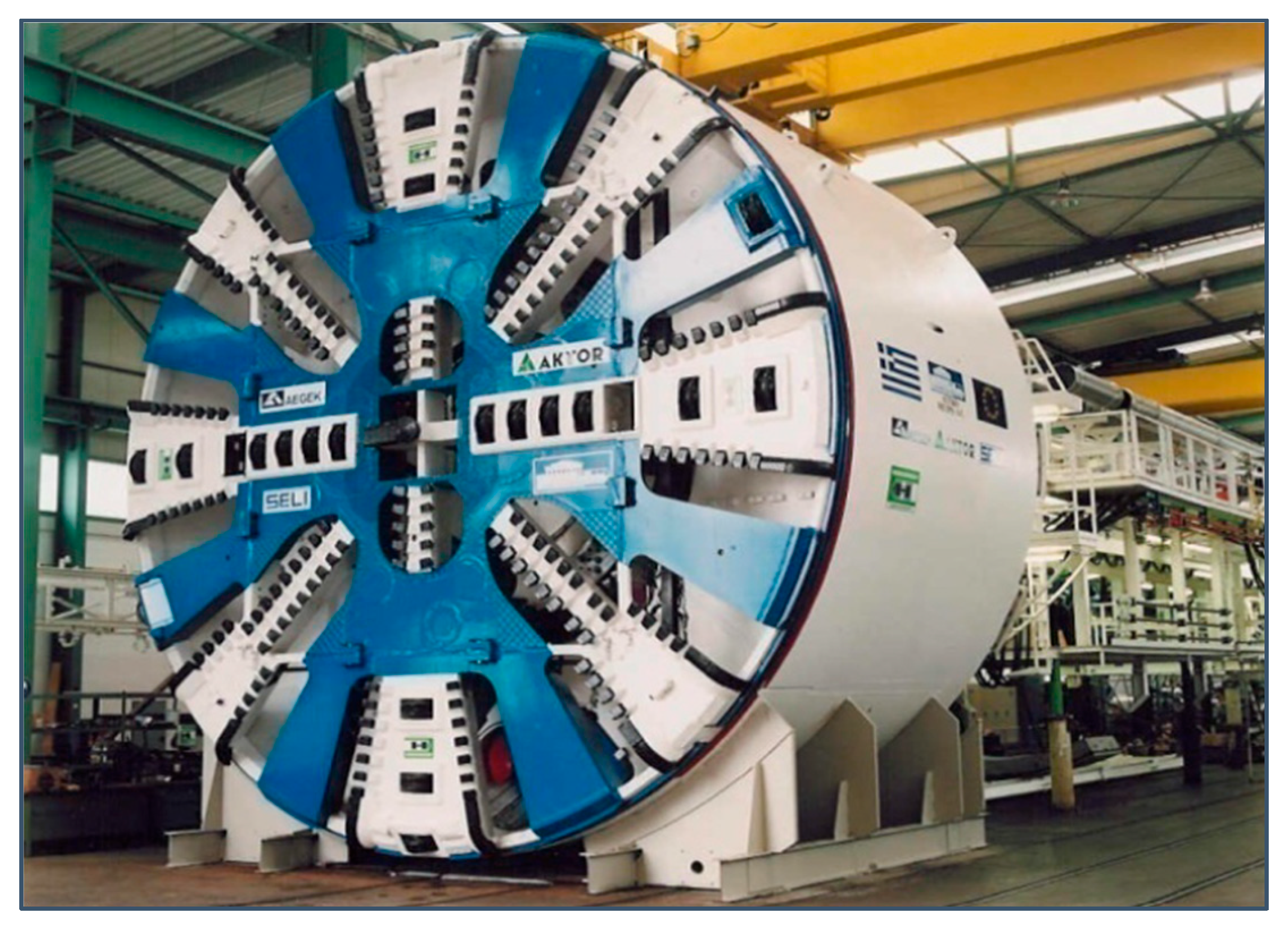
3.2. EPB Characteristics

The excavation of the single double-track tunnel was conducted using a Herrenknecht EPB machine with a 9.49 m diameter (Figure 3). The machine, with a maximum thrust force of 24,000 kNm and an instantaneous penetration rate of 60 mm/min, operated in closed excavation mode in challenging geotechnical conditions such as high-plasticity soils with low friction. Foam additives were used, with a foam volume ratio of 15–30% per cubic meter of excavated material and a foam expansion coefficient between 10:1 and 15:1 [22].

3.3. Geology of the Area

Geotechnical studies by Attiko Metro (Figure 4) reveal that the area’s geology consists mainly of cohesive calcareous materials, primarily limestone, varying from soft to hard. The region also includes silty clay mixed with sand and gravel, typically low or non-plastic. In some sections, the soil is soft and cohesive, occurring in three forms, namely (a) solid rock, (b) a fragmented rock–soil mixture, or (c) alternating sections of fragmented rock and soil with more soil-like properties [23].

4. Results

4.1. Surface Settlement Prediction Using ANN

The dataset from Attiko Metro included 61 records detailing TBM operational characteristics, geotechnical conditions, and tunnel geometric details. While we acknowledge that 61 records are not the best-case scenario for comprehensive analysis, they provided sufficient data for applying the O’Reilly and New theory [24]. The Peck constant (K) was calculated at 0.50 based on retrospective interval analysis and empirical data. To enhance measurement accuracy, parametric assessments were conducted for volume loss values ranging from 0.1% to 0.8%, aligning predictions with actual measurements in uncertain areas (Table 1). Details of operational and geometrical characteristics along with geotechnical conditions are presented in Table 2, Table 3 and Table 4.

Table 1. Empirical analysis and actual measurements of settlements and volume loss.

Volume Loss	Empirical Analysis	FEM Method	Range of Actual Settlements	Avg. of Actual Settlements	Actual Volume Loss
0.1%	−3 mm	−3 mm	from −1.80 mm to −22 mm	−8.52 mm	0.3–0.4%
0.2%	−6 mm
0.3%	−9 mm	−7 mm
0.4%	−12 mm
0.5%	−15 mm
0.6%	−18 mm
0.7%	−21 mm
0.8%	−24 mm

Table 1. Empirical analysis and actual measurements of settlements and volume loss.

Volume Loss	Empirical Analysis	FEM Method	Range of Actual Settlements	Avg. of Actual Settlements	Actual Volume Loss
0.1%	−3 mm	−3 mm	from −1.80 mm to −22 mm	−8.52 mm	0.3–0.4%
0.2%	−6 mm
0.3%	−9 mm	−7 mm
0.4%	−12 mm
0.5%	−15 mm
0.6%	−18 mm
0.7%	−21 mm
0.8%	−24 mm

TBM operational parameters are critical for assessing performance, efficiency, and challenges during tunnel excavation. Monitoring and optimizing these inputs ensure safer and more effective operations. Key parameters include the following:

• Head torque (MNm): rotational force on the cutting head, indicating excavation resistance and safe operating limits.
• Head thrust (kN): axial force at the tunnel face, reflecting the machine’s ability to advance through various geological conditions.
• Face pressure (bar): maintains tunnel stability and prevents collapses by applying pressure to the tunnel face.
• Penetration speed (mm/rev): tracks advancement per rotation, reflecting excavation efficiency.
• Grout pressure (bar): stabilizes surrounding soil and prevents settlement through controlled grout injection.
• Screw conveyor speed (rpm): determines material removal efficiency and overall progress.
• Grout volume (L): ensures ground stability and prevents water ingress through precise grout injection.
• Excavated soil (tn/h): indicates soil removal rate, reflecting machine productivity.
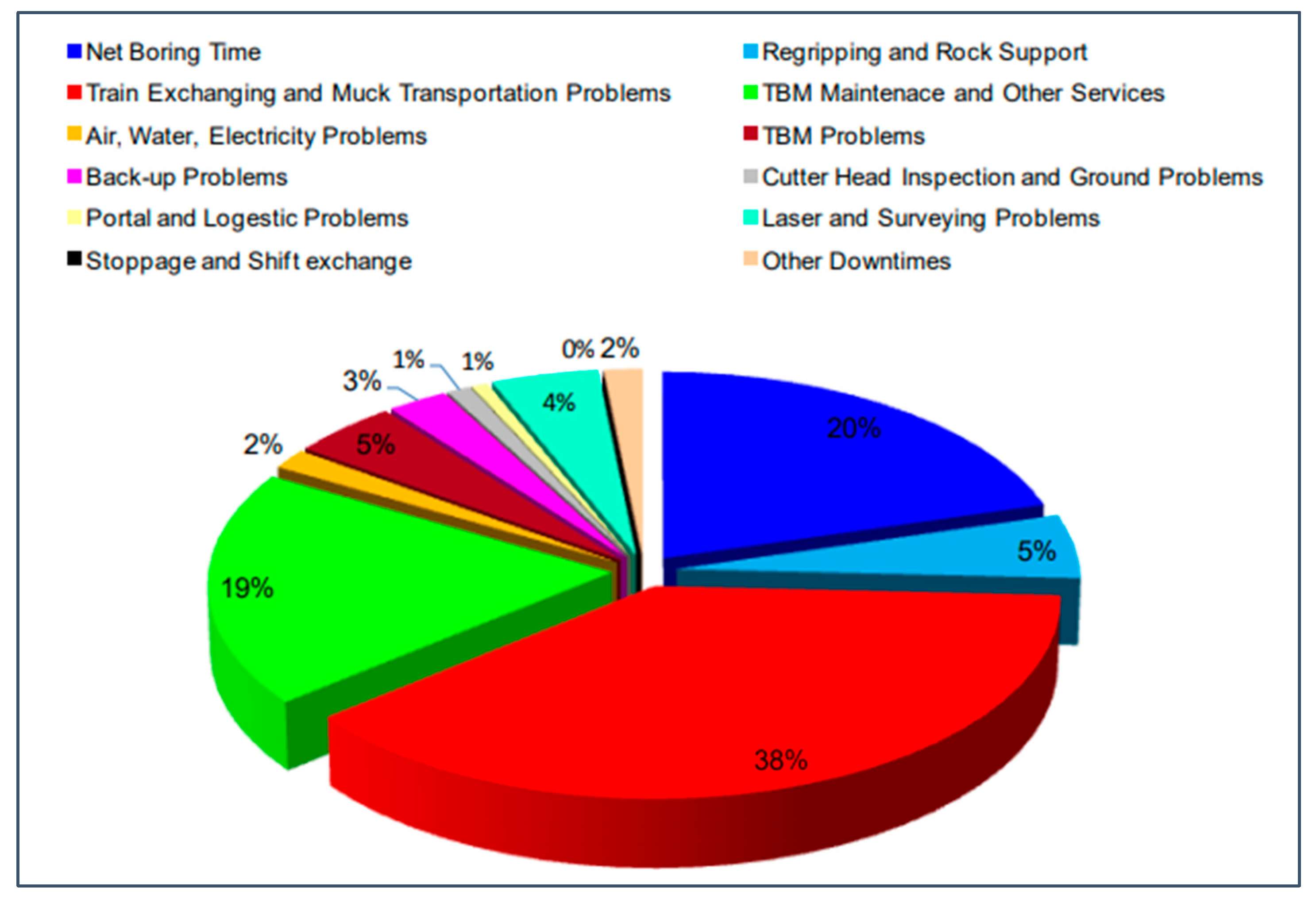
• Stop time (min): reducing stoppages enhances productivity, accelerates completion, and minimizes ground settlement risks.

Table 2. Description table of TBM operational parameters.

TBM Operational Parameters	Min	Max	Mean	Std.
Head torque (MNm)	7.10	13.50	9.98	1.32
Head thrust (kN)	14,514	23,842	19,166	2119
Face pressure (bar)	0.60	1.81	1.41	0.20
Penetration speed (mm/rev)	13	23	18.66	2.18
Grout pressure (bar)	1.5	4.0	2.5	0.5
Screw conveyor (rpm)	2	4.3	2.66	0.30
Grout volume (L)	22,138	4122	6976	1611
Excavated soil (tn/h)	107	245	199	25
Stop time (min)	3570	36	131.5	428.6

Table 2. Description table of TBM operational parameters.

TBM Operational Parameters	Min	Max	Mean	Std.
Head torque (MNm)	7.10	13.50	9.98	1.32
Head thrust (kN)	14,514	23,842	19,166	2119
Face pressure (bar)	0.60	1.81	1.41	0.20
Penetration speed (mm/rev)	13	23	18.66	2.18
Grout pressure (bar)	1.5	4.0	2.5	0.5
Screw conveyor (rpm)	2	4.3	2.66	0.30
Grout volume (L)	22,138	4122	6976	1611
Excavated soil (tn/h)	107	245	199	25
Stop time (min)	3570	36	131.5	428.6

Geotechnical parameters are crucial for assessing soil properties during TBM tunneling, directly influencing performance, safety, and settlement predictions. Key parameters include the following:

• Cohesion (c) in face area (kN): Measures soil strength at the tunnel face. Higher cohesion enhances stability, reducing collapse risk and aiding safe excavation.
• Cohesion (c) in overburden (kN): Refers to soil strength above the tunnel. Increased cohesion minimizes deformation and settlement risks.
• Angle of friction (φ) in face area: Represents soil resistance to movement at the tunnel face. A higher angle improves stability and reduces collapse risk.
• Angle of friction (φ) in overburden: Indicates soil resistance above the tunnel. A higher angle enhances overall stability and reduces settlement likelihood.

Table 3. Description table of TBM geotechnical parameters.

Geotechnical Parameters	Min	Max	Mean	Std.
Cohesion c in face area (c_e) (kN)	52.4	74.8	62.1	5.6
Cohesion c in overburden (c_o) (kN)	76.1	94.8	85.3	4.8
Angle of friction φ in face area (f_e)	35.2	41.6	36.1	0.8
Angle of friction φ in overburden (f_o)	36.1	40.3	37.8	1.4

Table 3. Description table of TBM geotechnical parameters.

Geotechnical Parameters	Min	Max	Mean	Std.
Cohesion c in face area (c_e) (kN)	52.4	74.8	62.1	5.6
Cohesion c in overburden (c_o) (kN)	76.1	94.8	85.3	4.8
Angle of friction φ in face area (f_e)	35.2	41.6	36.1	0.8
Angle of friction φ in overburden (f_o)	36.1	40.3	37.8	1.4

Geometrical parameters are critical for designing and executing TBM tunneling projects. They influence construction methods, safety, and logistical planning to align with site conditions. Key parameters include the following:

• Overburden (m): Depth of soil or rock above the tunnel. It determines the load and pressure on the tunnel, influencing stability and design.
• Distance to water table (m): Vertical distance from the tunnel invert to the water table. A shallow water table increases seepage risks, while a deeper one may require enhanced waterproofing.
• Distance from shaft (m): Distance from the tunnel to the access point. A shorter distance can affect TBM launching and cause ground disturbance, while greater distances may lead to ground stress and surface settlements.

Table 4. Description table of TBM geometrical parameters.

Geometrical Parameters	Min	Max	Mean	Std.
Overburden (m)	12.87	15.48	14.31	0.77
Distance to water table (tunnel invert to WT) (m)	−20.6	−17.2	−19.1	1.0
Distance from shaft (m)	0.0	283.5	131.7	83.1

Table 4. Description table of TBM geometrical parameters.

Geometrical Parameters	Min	Max	Mean	Std.
Overburden (m)	12.87	15.48	14.31	0.77
Distance to water table (tunnel invert to WT) (m)	−20.6	−17.2	−19.1	1.0
Distance from shaft (m)	0.0	283.5	131.7	83.1

To optimize neural network input processing, the data were normalized using the MinMaxScaler library. This common data science technique scales features to a range of 0 to 1, preserving measurement relationships without unit-related issues.

4.2. Model Development and Results

In this case study, four feedforward ANN models were developed, testing various architectures (layers, neurons, learning rates), batch sizes, epochs, and training/validation checks. The dataset, though small, was split 80% for training and 20% for testing, ensuring the model had no prior knowledge of the test data. Normalization was performed before the split to maintain accurate scaling, with maximum values derived from the training data.

After experimenting with multiple architectures, the final network (Figure 5) featured 16 input neurons with ReLU activation, two hidden layers (32 neurons in the first, 16 in the second), and one output neuron with linear activation to estimate maximum surface settlement (16 × 32 × 16 × 1). The Adam optimizer with an initial learning rate of 0.001 was used. To enhance convergence and prevent overfitting, a “Reduce Learning Rate on Plateau” strategy adjusted the learning rate when performance stopped improving, and early stopping halted training when validation performance plateaued, ensuring efficient resource use.

Four ANN models were developed to assess feature impacts, applying a simplified SHAP approach as follows:

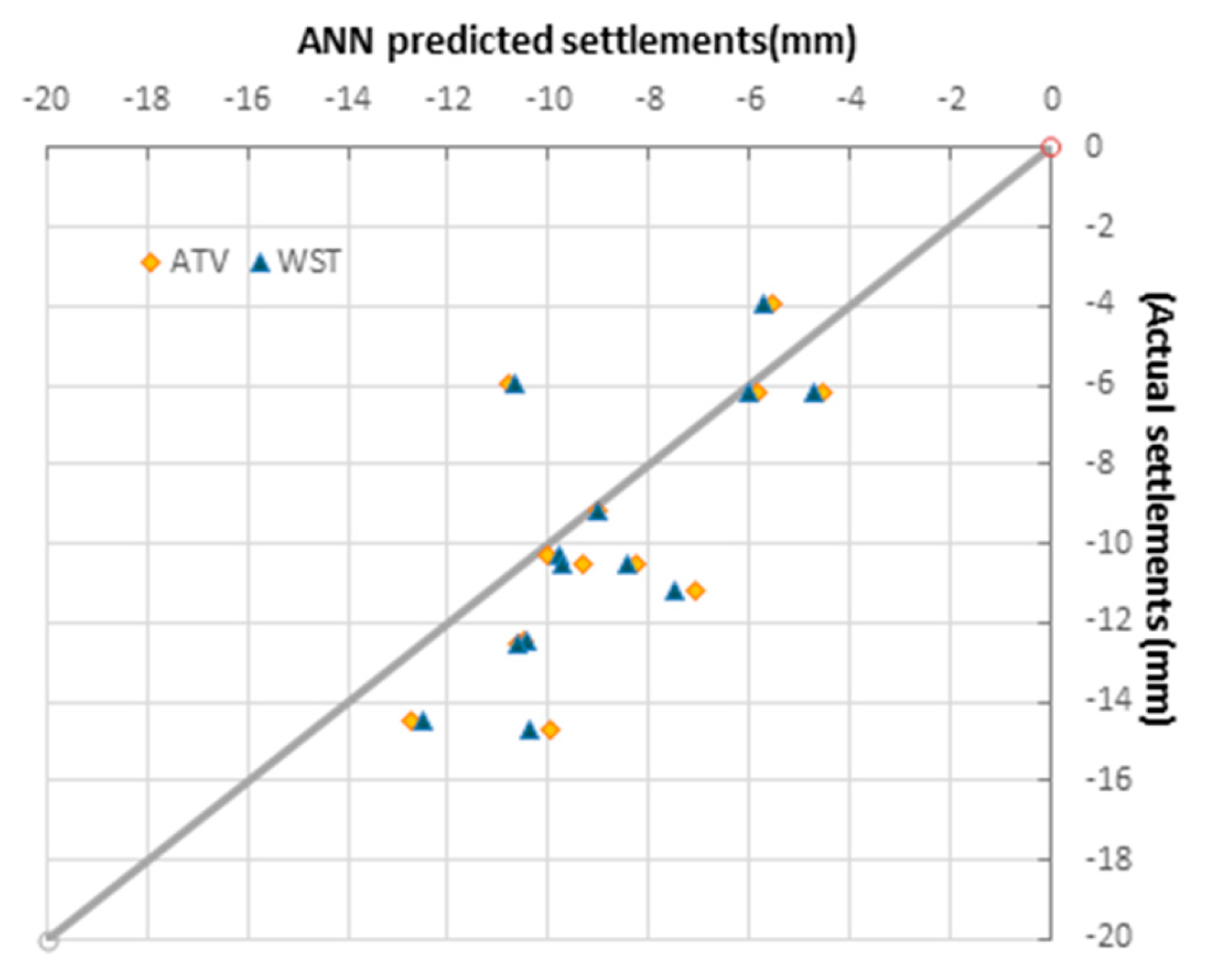
• ATV (all the variables): model with all features.
• WST (without stop time): model excluding the stop time parameter.
• WGV (without grout volume): model excluding the grout volume parameter.
• WES (without excavated soil): model excluding the excavated soil parameter.

Models were trained using the mean square error (MSE), with results also presented as the root mean square error (RMSE) and average prediction accuracy for comparison (

Table 5. MSE and RMSE training and test model results along with the avg. accuracy of the test results.

Models	MSE (mm)		RMSE (mm)		Average Accuracy
	Train	Test	Train	Test	Test
“ATV”	0.004	0.037	0.020	0.193	80.10%
“WST”	0.010	0.018	0.100	0.135	80.70%
“WGV”	0.005	0.038	0.070	0.196	80.02%
“WES”	0.012	0.023	0.109	0.152	79.30%

). All models performed well, achieving an average prediction accuracy above 79%, highlighting their potential for estimating surface settlements and providing tunneling engineers with a valuable decision-making tool.

The ATV and WST models emerged as the top performers, but their comparative effectiveness for predicting maximum settlements requires closer examination. Figure 6 illustrates this comparison with the gray line x = y representing perfect alignment between predicted and actual values. Points closer to this line indicate higher prediction accuracy. Overall, the WST model (aqua) slightly outperforms ATV, particularly in the mid-to-lower range of maximum settlements, where both models perform well.

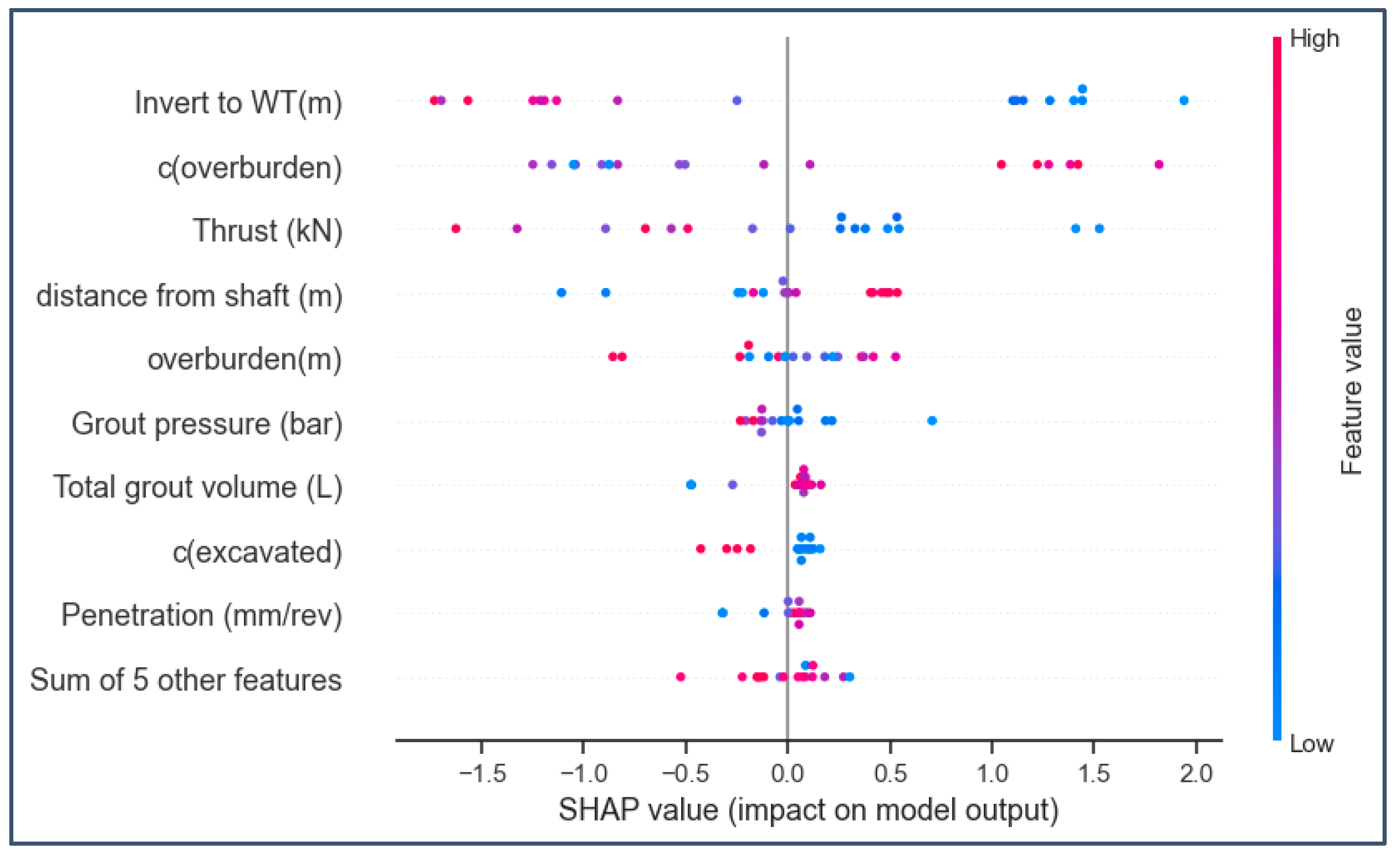
4.3. SHapley Additive exPlanations (SHAP)

The waterfall plot in Figure 7 illustrates how individual features contribute to the model’s prediction for a specific example. The baseline value, E[f(X)] = −7.75, represents the model’s average prediction across all feature combinations and serves as a reference point. The predicted value, f(x) = −4.766 (top right corner), is the model’s output for this specific input. The difference between f(x) and E[f(X)] is explained by the sum of the Shapley values for all features. The y-axis lists the features and their values for the analyzed datapoint. Red and blue arrows represent SHAP values, indicating whether a feature increases (red) or decreases (blue) the prediction, with absolute SHAP values showing the magnitude of each feature’s impact. In this case, cohesion of the overburden (kN) had the largest effect, followed by distance from the invert to WT (m) and the distance from the shaft (m). Notably, the cohesion of the overburden also made the smallest contribution in this instance. SHAP values are datapoint-specific and vary across observations.

The beeswarm plot (Figure 8) ranks features by their overall impact on predictions and visualizes how feature values affect outcomes. Each dot represents an observation, with the horizontal axis showing the SHAP value (feature contribution) and color indicating value levels (red for higher, blue for lower). The plot highlights feature relationships and their influence. For instance, higher “Invert to WT (m)” values strongly negatively impact predictions, while lower values contribute positively. Conversely, high cohesion (kN) in the overburden has a significant positive effect, while low values are negative. The “Penetration Speed (mm/rev)” feature shows minimal impact regardless of its value. Features are ranked by global importance, with the most influential at the top. This visualization effectively captures global feature impacts and local contributions across observations.

The decision plot (Figure 9) illustrates how features contribute to a model’s prediction. The x-axis represents the model’s output (settlements) in log odds, while the y-axis lists features in descending order of importance. SHAP values accumulate as you move from the bottom (expected value) to the top, showing each feature’s contribution to the final prediction. The plot begins at the base value and each feature pushes the prediction higher or lower. For example, the “Invert to WT (m)” feature consistently increases the prediction by 0.547 mm. While informative for understanding feature impacts, the plot is more effective when combined with other visualizations.

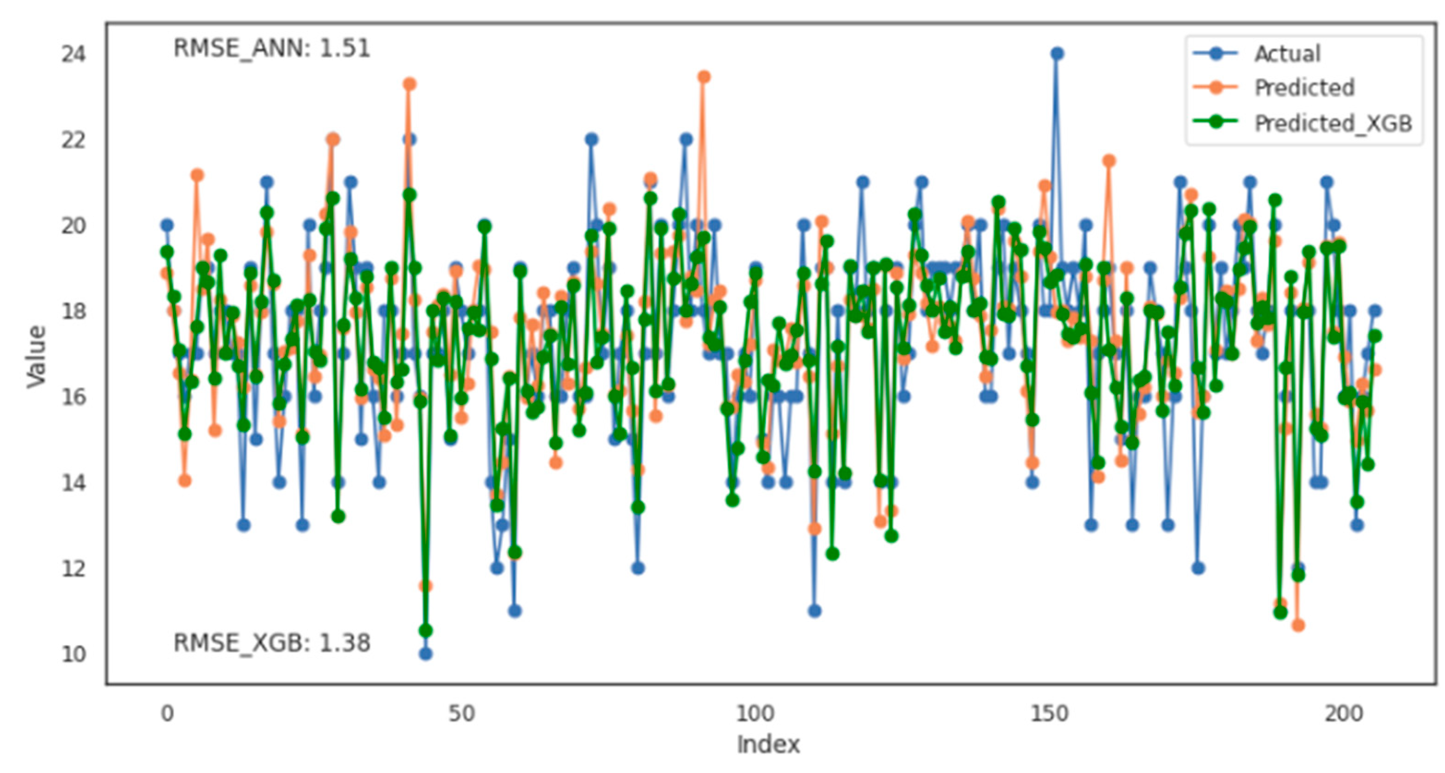
4.4. Penetration Rate Prediction Using ANN and XGBR

Two machine learning models, ANN and XGBR, were developed to predict the TBM’s penetration rate (PR) over a distance of 1624 m. The dataset, initially containing 1164 rows and 23 features, was normalized using the standard scaler (Equation (4)), where “u” is the mean of the training data and “s” represents the standard deviation of the training samples, with outliers (values > 3 standard deviations from the mean) removed, resulting in a final dataset of 1026 rows and 15 features.

$$z=\left(x-u\right)∕s$$

(4)

Feature selection was guided by Pearson correlation coefficients, and

Table 6. Description table of the model’s input parameters.

TBM Operational Parameters	Min	Max	Mean	Std.
TORQUE CW [MNm]	4.30	13.50	9.77	1.47
WORKING PRESSURE CW [bar]	53.00	169.00	122.35	18.27
TOTAL FORCE TC [kN]	5930.00	26,118.00	17,903.09	2869.86
SPEED TC [mm/min]	8.00	24.00	17.17	2.19
TORQUE SC [kNm]	0.00	122.00	78.47	14.74
WORKING_PRESSURE SC [bar]	0.00	154.00	98.96	18.65
PRESSURE GI [bar]	0.02	3.55	1.97	0.53
TOTAL GROUT A [L]	1011.00	8817.00	6333.44	500.90
TOTAL GROUT B [L]	107.00	621.00	476.27	43.75
A/B VOLUME	2.14	17.67	13.36	1.16
EXCAVATING [t/h]	29.00	252.00	182.44	32.06
FACE PRESSURE EP [bar]	0.00	1.97	1.29	0.28
AD PERCENTAGE	0.10	0.80	0.61	0.09
RING PERCENTAGE	0.12	0.58	0.30	0.06
STOP PERCENTAGE	0.00	0.55	0.09	0.10

summarizes the input parameters. The target variable was SPEED T.C., with features such as AD. PERCENTAGE, RING PERCENTAGE, and STOP PERCENTAGE representing time proportions for TBM advancement, ring segment placement, and inactivity.

4.5. Model Development and Results in Penetration Rate Prediction

The dataset was split 80–20 for training and testing, reserving 20% of the training set for validation. The XGBR model underwent hyperparameter tuning using GridSearchCV, while the ANN model adopted a simple architecture (15 × 64 × 32 × 1) with a ReLU activation function (except in the output layer) and Adam optimizer (initial learning rate: 0.001). Techniques like a custom learning rate scheduler and EarlyStopping were employed to enhance convergence and prevent overfitting. While Huber loss was considered for its robustness against outliers, the MSE was chosen as the loss function for better alignment with regression objectives. The ANN was trained for 500 epochs with close monitoring of validation metrics. Results, as summarized in

Table 7. Metrics for the training and testing process for the two models.

Models	MSE (mm/min)		RMSE (mm/min)		Wasserstein Distance
	Train	Test	Train	Test	Train	Test
XGB	0.38	1.90	0.62	1.38	0.33	0.42
ANN	1.06	2.26	1.03	1.50	0.30	0.40

, indicate both models performed well. The Wasserstein distance (earth mover’s distance, EMD) [25], was calculated to compare the distribution of predictions to the target distribution. The ANN achieved an EMD of 0.337 and the XGBoost model achieved 0.309, indicating a close match between predicted and actual distributions (Figure 10). The slightly lower EMD for XGBoost suggests it replicates the target distribution marginally better than the ANN model.

While EMD highlights the models’ ability to preserve statistical characteristics like mean, variance, and skewness, pointwise accuracy metrics such as the RMSE and MAE are necessary for evaluating individual prediction errors. Low values in these metrics would further validate the models’ accuracy.

The distribution plots (Figure 11) compare the ANN and XGBoost predictions against actual values, highlighting good alignment for both models. While ANN predictions show slight deviations in the tails, XGBoost predictions exhibit closer overlap with the actual distribution, as evidenced by its smaller Wasserstein distance. Both models display similar statistical properties, with XGBoost demonstrating marginally better accuracy in capturing the overall distribution.

The small Wasserstein distances reflect strong model performance, with XGBoost slightly outperforming the ANN. However, selecting the “better” model should also consider factors like computational efficiency, robustness, interpretability, and pointwise accuracy, alongside Wasserstein distance.

In Figure 12, a comparison of the models is depicted, showcasing their ability to accurately track the actual target trend (generalization).

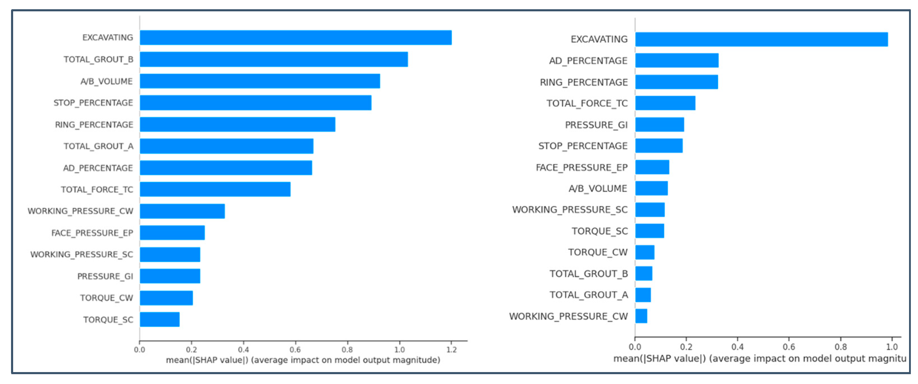
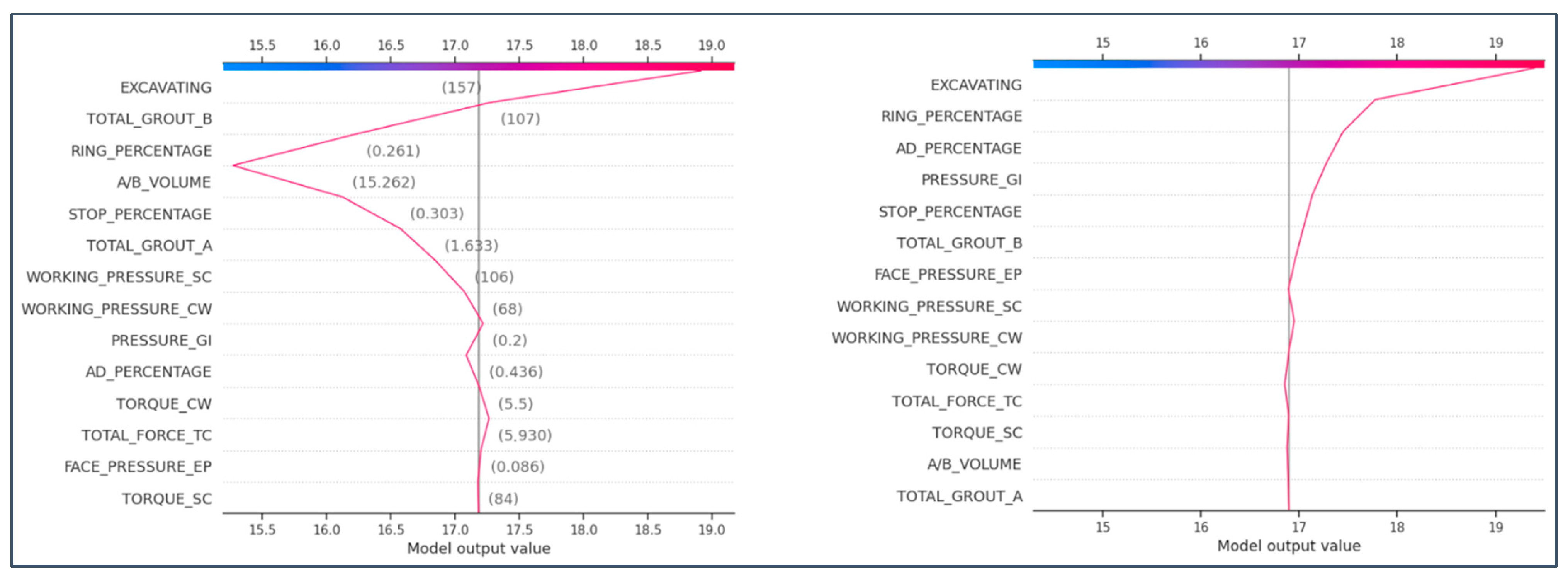
4.6. SHapley Additive exPlanations (SHAP) in Penetration Rate Prediction

The SHAP library was applied to both models, using Tree Explainer for XGBR and Deep Explainer for ANN to enhance interpretability and compare model complexities. This comparison provides a deeper understanding of how each model processes information and makes predictions.

The SHAP summary plots (Figure 13) reveal differences in how the models rank impactful parameters and their associated mean SHAP values. These variations are minor and align with theoretical engineering insights, reinforcing the validity of both models. Both summary plots highlight the importance of features like AD. PERCENTAGE, RING PERCENTAGE, and STOP PERCENTAGE, emphasizing the correlation between PR delays and time-related factors.

Both models also rank grout-related features (e.g., TOTAL GROUT B [L], A/B VOLUME, PRESSURE_GI) highly, following the consistently top-ranked EXCAVATING feature. Grout pressure is critical for stabilizing soil, reducing friction, and maintaining tunnel face balance to prevent collapse. This alignment between ML findings and traditional engineering principles underscores the robustness and explanatory power of both fields.

The decision plots in Figure 14 reflect the key concepts from the summary plots. In the ANN plot (left), the high variability in impacts mirrors the summary plot, where multiple parameters significantly influence predictions. In contrast, the XGBR plot (right) shows a more consistent impact, with fewer dramatic changes after the initial high values.

Comparing features like EXCAVATING or RING PERCENTAGE from the top five highlights these differences. On both sides of the gray line (representing the model’s output), the ANN model demonstrates greater sensitivity to these parameters, while the XGBR model responds more steadily. This variation stems from the models’ training methods; XGBR’s hierarchical tree structure produces smoother responses, whereas ANN’s complex weight adjustments increase sensitivity to specific parameters.

In the beeswarm plot (Figure 15), note that the x-axis ranges differ between the ANN (left) and XGBR (right) models. Thus, a high value on one plot does not directly correspond to the same high value on the other. However, the overall parameter behavior remains consistent. For instance, in both plots, low values of the EXCAVATING feature consistently have a low-to-medium negative impact on the model’s output.

An interesting distinction lies in how features with minimal contributions are presented. In the XGBR plot, these features appear after the top five, while in the ANN plot, they emerge later, after the eighth feature. This reflects the models’ differing sensitivities to certain parameters during training.

4.7. Other Interpretable Models

Application of Integrated Gradients (IGs) in the ANN model.

Integrated gradients (IGs) comprise a technique used in ANNs to attribute each input feature’s contribution to a model’s prediction. It is a core method in Explainable AI (XAI), particularly effective for explaining complex deep learning models. Unlike standard gradient-based methods that assess output sensitivity to small input changes, IGs integrate gradients along a path from a baseline input (e.g., all-zero or blurred data) to the actual input.

IGs compute feature importance by comparing the actual input to the baseline and integrating the gradients of the model output with respect to input features along this path. The result provides a comprehensive measure of each feature’s contribution.

Mathematically, IGs are calculated as the product of a feature’s difference from its baseline and the integral of the model output’s gradient over the path from baseline to input. This method adheres to the two following principles:

• Sensitivity: features with no effect on the prediction receive zero attribution.
• Completeness: the sum of all feature attributions equals the difference between the model’s output at the actual input and the baseline.

IGs are widely applied to identify key predictive features, debug models, ensure fairness by analyzing sensitive attributes, and provide interpretable insights into black box models. By integrating gradients over a path, it avoids the noise and instability of single-gradient calculations, offering a smooth and robust explanation method.

Figure 16 provides a comparison of IGs and SHAP’s Deep Explainer, highlighting key observations.

High positive attribution values: Features like PRESSURE_GI (2.02), the highest positive attribution, significantly contribute to the model’s output, indicating a strong influence on predictions. Other features, such as WORKING PRESSURE_CW (1.60) and RING_PERCENTAGE (0.34), also positively impact the output, albeit to a lesser extent.

Negative attribution values: features like A/B_VOLUME (−0.96) and STOP_PERCENTAGE (−0.69) have substantial negative attributions, meaning they significantly decrease the predicted output, reflecting inverse importance.

Neutral or insignificant features: features such as EXCAVATING (0.02) and TOTAL_FORCE_TC (0.04) show minimal attribution, suggesting negligible impact on the model’s predictions.

Mixed contributions: AD_PERCENTAGE (−0.10) has a small negative contribution, slightly reducing the output without significant impact.

The model heavily relies on PRESSURE_GI, a key driver of the target variable, likely reflecting a critical operational or physical property. Negative contributors like A/B_VOLUME and STOP_PERCENTAGE may represent factors that oppose the desired outcome, warranting further investigation or mitigation. Features with negligible impact, such as EXCAVATING and TOTAL_FORCE_TC, appear less relevant to the model and dataset.

XGBoost’s plot_importance.

The XGBoost plot_importance function visualizes feature importances using metrics such as the following:

• Weight: the number of times a feature is used to split data across all trees.
• Gain: the average information gain from splits involving the feature.
• Cover: the average number of samples covered by splits using the feature.

From the visualization (Figure 17—right), feature importance based on gain in an XGBoost model highlights how specific features improve model accuracy. PRESSURE_GI is the most impactful, playing a critical role in performance, followed by TOTAL_GROUT_B and TORQUE_SC, which also contribute significantly but to a lesser extent. Features like STOP_PERCENTAGE, TORQUE_CW, and TOTAL_FORCE_TC provide moderate support, while EXCAVATING, WORKING_PRESSURE_CW, and AD_PERCENTAGE show minimal impact and could be considered for removal to simplify the model. The sharp drop in importance after the top three features underscores the disproportionate contribution of the key variables.

In the weight-based importance chart (Figure 17—left), TORQUE_CW and TORQUE_SC are the most frequently used features, with weights of 184 and 172, respectively, indicating their essential role in splitting data and capturing patterns. TOTAL_GROUT_B and FACE_PRESSURE_EP follow as significant contributors, while PRESSURE_GI, A/B_VOLUME, and WORKING_PRESSURE_CW provide moderate support. Features like AD_PERCENTAGE and EXCAVATING have the lowest weights, reflecting minimal relevance to the target variable.

Notably, PRESSURE_GI, ranked first in the gain chart, is fifth in the weight chart, illustrating the distinction between weight, which measures feature usage frequency, and gain, which evaluates the quality of contributions. TORQUE_CW and TORQUE_SC are consistently prioritized, emphasizing their direct relevance. Lower-weight features, such as EXCAVATING, may be removed if they fail to enhance performance. Features like TOTAL_GROUT_B and FACE_PRESSURE_EP provide reliable patterns that the model leverages for predictions.

While the weight chart emphasizes usage frequency, the gain chart reflects the actual contribution to predictive power. Balancing these perspectives provides a comprehensive understanding of the model, aiding in feature selection and interpretability.

5. Conclusions

The integration of the SHAP library, based on Shapley values from game theory, provides clear insights into how models like XGBR (using XGB—Tree Explainer) and ANN (using Deep Explainer) make decisions. These explainers consistently identify key parameters, their impact on predictions, and the magnitude of their influence, with minimal discrepancies across numerous examples. In addition to SHAP, integrated gradients (IGs) were applied to the ANN model, and XGBoost’s plot_importance function was used for the XGB model. Both methods offer valuable insights into feature importance and contributions to predictions.

SHAP is often preferred for its game theory foundation, ensuring fairness and comprehensiveness in attributing feature contributions. Unlike methods providing relative or gradient-based importance, SHAP offers a unified approach for calculating each feature’s specific impact while maintaining consistency across models and datasets. Its flexibility, along with local and global interpretability, makes SHAP indispensable for model explainability.

Machine learning models not only improve predictions for PR and surface settlements but also enhance risk and safety assessments, equipping engineers with tools to manage uncertainties in underground construction. SHAP bridges the gap between understanding and trusting models, addressing the “black box” nature of ANNs by allowing engineers to trace every step of a prediction. This interpretability advances model application in real-world projects, supporting the design and construction of durable underground structures.

As the construction industry evolves, SHAP’s application in tunneling represents a significant leap forward, offering engineers tools that not only predict outcomes but also explain the complex dynamics of underground projects. This ensures a promising future for interpretable machine learning in construction.

References

1. Jamshidi, A. Prediction of TBM penetration rate from brittleness indexes using multiple regression analysis. Model. Earth Syst. Environ. 2018, 4, 383–394. [Google Scholar] [CrossRef]
2. Benardos, A.G.; Kaliampakos, D.C. Modelling TBM performance with artificial neural networks. Tunn. Undergr. Space Technol. 2004, 19, 597–605. [Google Scholar] [CrossRef]
3. Ghasemi, E.; Yagiz, S.; Ataei, M. Predicting penetration rate of hard rock tunnel boring machine using fuzzy logic. Bull. Eng. Geol. Environ. 2014, 73, 23–35. [Google Scholar] [CrossRef]
4. Feng, S.; Chen, Z.; Luo, H.; Wang, S.; Zhao, Y.; Liu, L.; Ling, D.; Jing, L. Tunnel boring machines (TBM) performance prediction: A case study using big data and deep learning. Tunn. Undergr. Space Technol. 2021, 110, 103636. [Google Scholar] [CrossRef]
5. Benardos, A. Artificial intelligence in underground development: A study of TBM performance. In Proceedings of the WIT Transactions on the Built Environment, The New Forest, UK, 8–10 September 2008; Volume 102, pp. 21–32. [Google Scholar] [CrossRef]
6. Alvarez Grima, M.; Bruines, P.A.; Verhoef, P.N.W. Modeling tunnel boring machine performance by neuro-fuzzy methods. Tunn. Undergr. Space Technol. 2000, 15, 259–269. [Google Scholar] [CrossRef]
7. Yagiz, S.; Karahan, H. Prediction of hard rock TBM penetration rate using particle swarm optimization. Int. J. Rock Mech. Min. Sci. 2011, 48, 427–433. [Google Scholar] [CrossRef]
8. Jahed Armaghani, D.; Mohamad, E.; Narayanasamy, M.; Narita, N.; Yagiz, S. Development of hybrid intelligent models for predicting TBM penetration rate in hard rock condition. Tunn. Undergr. Space Technol. 2017, 63, 29–43. [Google Scholar] [CrossRef]
9. Chen, T.; Guestrin, C. XGBoost: A Scalable Tree Boosting System. In Proceedings of the KDD ’16: The 22nd ACM SIGKDD International Conference on Knowledge Discovery and Data Mining, San Francisco, CA, USA, 13–17 August 2016; pp. 785–794. [Google Scholar] [CrossRef]
10. Zhou, J.; Qiu, Y.; Zhu, S.; Armaghani, D.J.; Khandelwal, M.; Mohamad, E.T. Estimation of the TBM advance rate under hard rock conditions using XGBoost and Bayesian optimization. Undergr. Space 2021, 6, 506–515. [Google Scholar] [CrossRef]
11. Ninic, J.; Bui, H.-G.; Koch, C.; Meschke, G. Computationally Efficient Simulation in Urban Mechanized Tunneling Based on Multilevel BIM Models. J. Comput. Civ. Eng. 2019, 33. [Google Scholar] [CrossRef]
12. Zhao, Z.; Gong, Q.; Zhang, Y.; Zhao, J. Prediction model of tunnel boring machine performance by ensemble neural networks. Geomech. Geoengin. 2007, 2, 123–128. [Google Scholar] [CrossRef]
13. Kannangara, K.K.P.M.; Zhou, W.; Ding, Z.; Hong, Z. Investigation of feature contribution to shield tunneling-induced settlement using Shapley additive explanations method. J. Rock Mech. Geotech. Eng. 2022, 14, 1052–1063. [Google Scholar] [CrossRef]
14. Hu, M.; Zhang, H.; Wu, B.; Li, G.; Zhou, L. Interpretable predictive model for shield attitude control performance based on XGboost and SHAP. Sci. Rep. 2022, 12, 18226. [Google Scholar] [CrossRef] [PubMed]
15. Sirisena, G.; Jayasinghe, T.; Gunawardena, T.; Zhang, L.; Mendis, P.; Mangalathu, S. Machine learning-based framework for predicting the fire-induced spalling in concrete tunnel linings. Tunn. Undergr. Space Technol. 2024, 153, 106000. [Google Scholar] [CrossRef]
16. Flor, A.; Sassi, F.; La Morgia, M.; Cernera, F.; Amadini, F.; Mei, A.; Danzi, A. Artificial intelligence for tunnel boring machine penetration rate prediction. Tunn. Undergr. Space Technol. 2023, 140, 105249. [Google Scholar] [CrossRef]
17. Ralph Peck, B. Deep Excavations and Tunneling in Soft Ground. In 7th International Conference on Soil Mechanics and Foundation Engineering (Mexico), Mexico: International Society for Soil Mechanics and Geotechnical Engineering. 1969. Available online: https://www.issmge.org/publications/publication/deep-excavations-and-tunneling-in-soft-ground (accessed on 2 December 2024).
18. Guglielmetti, V.; Grasso, P.; Mahtab, A.; Xu, S. (Eds.) Mechanized Tunnelling in Urban Areas: Design Methodology and Construction Control, 1st ed.; CRC Press: Boca Raton, FL, USA, 2008; ISBN 978-0-203-93851-5. [Google Scholar]
19. Lundberg, S.; Lee, S.-I. A Unified Approach to Interpreting Model Predictions. arXiv 2017, arXiv:1705.07874. [Google Scholar] [CrossRef]
20. Lipovetsky, S.; Conklin, M. Analysis of Regression in Game Theory Approach. Appl. Stoch. Models Bus. Ind. 2001, 17, 319–330. [Google Scholar] [CrossRef]
21. Štrumbelj, E.; Kononenko, I. Explaining prediction models and individual predictions with feature contributions. Knowl. Inf. Syst. 2014, 41, 647–665. [Google Scholar] [CrossRef]
22. Koukoutas, S.; Sofianos, A. Settlements Due to Single and Twin Tube Urban EPB Shield Tunnelling. Ge-Otechnical Geol. Eng. 2015, 33, 487–510. [Google Scholar] [CrossRef]
23. Attiko Metro, S.A. AGHIOS DIMITRIOS—ELLINIKO Extension. Available online: https://www.emetro.gr/?page_id=4179&lang=en (accessed on 2 December 2024).
24. Settlements Above Tunnels in the United Kingdom—Their Magnitude and Prediction—Tunnels & Tunnelling International. Available online: https://www.tunnelsonline.info/news/settlements-above-tunnels-in-the-united-kingdom-their-magnitude-and-prediction-6733559 (accessed on 9 January 2024).
25. Kantorovich, L.V.; Rubinshtein, S.G. On a Space of Totally Additive Functions. Vestn. St. P. Univ. Math. 1958, 13, 52–59. [Google Scholar]
Figure 1. Typical TBM work distribution in Ghomroud tunnel.
Applsci 14 11394 g001
Figure 2. Schematic representation of the SHAP library function.
Applsci 14 11394 g002
Figure 3. The EPB machine used during the excavation of interval 5.
Applsci 14 11394 g003
Figure 4. Geotechnical parameters and a section of the geological background of the interval (Attiko Metro, 2007 [23]).
Applsci 14 11394 g004
Figure 5. Architecture of the ANN model “ATV” (16 × 32 × 16 × 1).
Applsci 14 11394 g005
Figure 6. Actual vs. predicted values of the two best performing models.
Applsci 14 11394 g006
Figure 7. A SHAP waterfall plot between an expected and predicted value of a single example.
Applsci 14 11394 g007
Figure 8. A SHAP beeswarm plot presenting the impact of every feature on the model’s output.
Applsci 14 11394 g008
Figure 9. A SHAP decision plot depicting observations converging at the expected value.
Applsci 14 11394 g009
Figure 10. Effort to transform predicted distributions to actual.
Applsci 14 11394 g010
Figure 11. Distribution plots for the two models in comparison to the actual.
Applsci 14 11394 g011
Figure 12. A generalization of the ANN (orange) and XGB (green) model—test dataset.
Applsci 14 11394 g012
Figure 13. SHAP summary plots on the average impact on the model’s output for the ANN model (left) and the XGBR model (right).
Applsci 14 11394 g013
Figure 14. A SHAP decision plot depicting observations converging at the expected value for the ANN model (left) and the XGBR model (right).
Applsci 14 11394 g014
Figure 15. A SHAP beeswarm plot presenting the impact of every feature on the model’s output for the ANN model (left) and the XGBR model (right).
Applsci 14 11394 g015
Figure 16. Application of integrated gradients (IGs) in the ANN model.
Applsci 14 11394 g016
Figure 17. XGBoost’s feature importance based on gain (right) and based on weight (left).
Applsci 14 11394 g017