Exposure to NO₂ and PM_2.5 While Commuting: Utility of Low-Cost Sensor

Featured Application

Personal exposure was assessed using low-cost sensors compared to stationary measurements. These findings highlight the influence of transport modes and seasonal conditions on real-time exposure to air pollution. The results highlight the necessity for targeted interventions—such as infrastructure improvements and regulatory measures—to reduce commuters’ exposure to traffic-related pollutants and enhance urban air quality.

Abstract

This study examines variations in personal exposure to PM_2.5 and NO₂ while commuting by bicycle, vehicle, and walking during heating and non-heating seasons in Gliwice, an industrial city in Upper Silesia, Poland. Understanding these variations is crucial for assessing health risks and developing effective mitigation strategies. Personal exposure was measured using low-cost sensors, while stationary measurements provided comparative background concentrations. The results indicate statistically significant seasonal differences in pollutant concentrations. NO₂ levels were higher during the heating season (mean: 30.84 µg/m³, median: 25.60 µg/m³) than in the non-heating season (mean: 22.61 µg/m³, median: 20.37 µg/m³; p = 0.025). In contrast, PM_2.5 concentrations were higher in the non-heating season (mean: 12.1 µg/m³) compared to the heating season (mean: 9.5 µg/m³; p = 0.032). Inhaled doses instead of concentrations evaluated the exposure of participants. The inhaled doses of NO₂ and PM_2.5 per km were significantly higher for walking (mean: 141.3 and 30.7 µg/km for the male participant; 77.9 and 31.6 µg/km for the female participant) than for bicycle and walking (p < 0.05). These findings underscore the impact of transport mode and seasonality on air pollution exposure, highlighting the necessity for targeted mitigation strategies to reduce commuters’ exposure to traffic-related pollutants.

1. Introduction

Physical activity is essential in preventing noncommunicable diseases in developed countries [1]. Compared to recreational physical activities, which require an individual to allocate time, utilitarian bicycling during commuting specifically enables physical activities with daily and necessary routines. Almost all commuter cycling falls into the ‘moderate intensity’ category of exercise, with an energy expenditure of approximately 4 MET (metabolic equivalent of task), or 5–8 times the energy expenditure at rest [2]. This level is about twice as intensive as walking and offers near-continuous activity. Cycling for transportation has many health-related advantages. According to Agarwal [3], cycling for 3 h per week results in a relative risk of 0.72, with a 28% reduction in all-cause mortality compared to non-cyclists. Results presented by Ma et al. [4] suggest that occasional cycling for transportation (less than 3 days/week) may not be able to generate significant benefits on mental well-being. However, regular bicycling for transportation (3 days/week or more) may reduce mental distress and boost life satisfaction. An excellent example is Sweden, where 19.2% of the working population meets the WHO’s global health recommendations, including moderate- to vigorous-intensity physical activity performed at least 30–60 min per day and more than 150 min of moderate-intensity activity per week [5], just through their bicycle commutes to work [6]. In Poland, 83% of the population knows how to ride a bike, which is more than the 63% global average. In total, 69% own one, and 44% use it at least once a week. However, Poles treat cycling as a sports activity rather than the primary mode of transport for a 2 km distance (18%) [7].

Despite Poles being more and more willing to implement eco-friendly solutions to their lifestyles, in the matter of transport, the changes go slower [8]. According to a report by the Polish Ministry of Climate and Environment conducted in March 2022, “Which mode of transport do you use most often to get to work?”, 47% of compatriots indicated the car. In comparison, survey results from 1995 and 2005 [9] stated a similar share in 1995, while in 2005, the car was the most frequent mode of transport for 78% of respondents from Polish districts with a high level of mobility.

According to the Parliament of the European Union (EU), the transport sector’s most serious challenge is significantly reducing its emissions and becoming more sustainable [10]. Among activities aimed at reducing air pollutant emissions from the transport sector at the regional and local scales, the extension of cycling infrastructure and promotion in cities are mentioned. When people choose to ride bikes instead of driving cars, they contribute to reducing the emissions of pollutants from vehicles. Promoting cycling for health reasons implies that the health benefits of cycling should outweigh the risks of cycling. Bikes do not emit pollutants. Therefore, society may benefit from a shift from private car use to bicycle use, making them a zero-emission mode of transportation. Bikes are recommended as an active transport mode, reducing air pollution. However, it is essential to note that disadvantages to individuals may occur. For example, the risks of being involved in traffic accidents increase [2].

Additionally, in areas with high levels of air pollution, cycling can expose people to higher levels of pollutants due to increased respiration rates. For automobile traffic, the characteristic pollutants are NO₂ and PM_2.5 [11]. Both are derived from combustion processes and increase oxidative stress [12]. NO₂ is often treated as a surrogate for PM [13,14]. On the other hand, 14% to 27% of the measured secondary PM_2.5 is generated from the NOx set of reactions [15,16].

On 16 February 2023, the European Parliament published a resolution on developing an EU cycling strategy and called to designate 2024 as the European Year of Cycling [17]. Following this idea, on 25 February 2024, Metropolis GZM (associating 41 cities and municipalities with a total area of 2500 km², home to 2.1 million inhabitants) launched Metropolitan Bicycle, Poland’s most extensive urban bicycle system. The system will ultimately comprise 7000 bicycles and allow travel in 31 municipalities, starting with the eight largest cities in the region [18]. Metropolis GZM is a well-known European hotspot region for air pollution [19]. In total, 5 of the 15 most polluted cities in the EU are located in this region [20]. Given the individual and environmental benefits, the challenge for researchers is to promote cycling in countries such as Poland, where it is not common as a daily mode of transport. Apart from the need to provide adequate facilities for cyclists, one of the main problems is the perception of cycling as a safe mode of transport in regions of high air pollution. Hence, this article aims to investigate exposure to NO₂ and PM_2.5 while cycling/walking/driving during the heating and non-heating season. Literature reviews [21,22,23], including experimental studies that compare exposure to traffic air pollutants among active commuters (pedestrians or cyclists) and commuters using motorized transport, clearly indicate data gaps in Central and Eastern Europe.

This study presents the first research findings on active commuting in the most polluted region of Poland, with a specific focus on continuous, individualized air quality monitoring to enhance the estimation of personal exposure levels. The principal aim is to address critical data gaps concerning exposure to NO₂ and PM_2.5 by applying a novel methodological approach based on deploying low-cost, portable sensors. Incorporating low-cost sensor technology constitutes a significant technological innovation, enabling the collection of high-resolution, real-time exposure data that reflect the dynamic nature of individual activity patterns and varying microenvironments. This approach represents a substantial advancement over traditional reliance on fixed ambient monitoring stations, which are limited in capturing the true variability of personal exposure during active commuting. The study seeks to provide a robust basis for comprehensive health risk assessments (HRA), including the estimation of inhaled doses of NO₂ and PM_2.5. By delivering individualized exposure data, the research aims to more accurately evaluate whether the health benefits of active commuting, such as cycling or walking, outweigh the associated risks of air pollution exposure. Ultimately, by demonstrating the utility of low-cost sensor technology in environmental health studies, this research aspires to contribute to the broader adoption of cost-effective monitoring solutions, thereby facilitating improved population health outcomes in urban areas.

2. Materials and Methods

2.1. Study Area

The study was conducted between January and November 2022 in Gliwice, a city in the industrial region of Upper Silesia (4.5 million people) in southern Poland. Gliwice is a city with an area of 134.2 km² and a population exceeding 177,000. It ranks 19th among Poland’s largest cities in terms of area and population. Within the Metropolis GZM, it holds the fourth position in terms of population. Gliwice is recognized as a well-known European city with a high PM_2.5 concentration, ranking 8th among the 15 most polluted cities in the EU (Smart Air, 2024). In Poland, 78.8% of PM_2.5 emissions originate from residential, commercial, and institutional sources, 8.7% from agriculture, and 3.7% from transport.

Regarding NO₂ emissions, transportation accounts for 31.9% (with passenger cars comprising 86% of this segment), followed by energy supply (23.7%) and residential, commercial, and institutional activities (13.0%). Gliwice’s distinctive vehicular landscape is typified by a substantial number of vehicles and notable traffic intensity, notably featuring an aging fleet predominantly comprising gasoline- and diesel-powered vehicles. Specifically, vehicles exceeding 15 years of age represent over 50% and 70% of the total car and bus fleet, respectively [24]. The measurements were divided into two seasons according to moderate climate conditions (atmospheric temperature) and the significant role of residential emissions for heating purposes. The months from April to September were defined as non-heating seasons, while January to March and October to November were defined as heating seasons.

2.2. Study Design

The study was designed to assess the real-time exposure of two participants (male—person 1; female—person 2) to PM_2.5 and NO₂ while commuting to the University campus by three transportation modes: bicycle, vehicle, and walking. The measurements were systematically conducted on each regular working day during the study period (from January to November 2022), ensuring comprehensive coverage of typical daily conditions. The participants were not instructed or constrained in their choice of transportation mode; instead, they independently selected the means of transport based on their personal needs, preferences, circumstances, and weather conditions on a given day. This methodological decision was deliberate, aiming to capture natural variations in exposure levels under real-world conditions, thereby enhancing the ecological validity and practical applicability of the findings. Figure 1 presents the routes of journeys. During cycling, the participants used the available cycle paths. Gliwice currently offers access to a network comprising 126.5 km of dedicated cycling routes and pathways [25], corresponding to 0.71 m of cycle routes per capita. The distance puts Gliwice at the top of Polish cities; however, it is far from the European leaders, exceeding 1 m of cycle routes per capita [26,27]. The measurements of personal exposure to NO₂ and PM_2.5 were performed by a low-cost Flow 2 personal sensor (produced by Plume Labs, Paris, France).

The device has a light-scattering laser counter that measures particulate concentrations and a metal oxide sensor that measures gas concentrations. An application on the phone enables data recording as graphs and levels that can be uploaded. NO₂ concentrations are presented in ppb. Hence, in the article, NO₂ concentrations are converted to µg/m³ (the conversion factor is 1.91), while PM_2.5 is measured in μg/m³. The sampling frequency is fixed at 60 s. Self-calibration with cutting-edge machine-learning algorithms is contained in Flow’s proprietary firmware [28]. According to the manufacturer, the correlation coefficient for NO₂ with the reference device APNA370 NOx monitor (produced by HORIBA Corp., Kyoto, Japan) is in the range from 84 to 99% (average 96%), while for PM_2.5 the reference device was an AeroTrak 9306 Handheld Particle Counter (produced by TSI Incorporated, Shoreview, MN, USA) with correlation in the range from 87.3% to 97.0% (average 90.9%) [29]. It should be noted that manufacturers often achieve high correlations with reference-grade sensors under strictly controlled conditions, while the details of the calibration procedures are typically protected as trade secrets. However, under real-world conditions, the accuracy of many low-cost sensors generally falls within a ±10% range for most air pollutants. Furthermore, regardless of the precision of the calibration process, low-cost sensors are highly sensitive to meteorological factors and require an acclimatization period when the monitoring environment changes [30,31]. Among the studies published to date, Crnosija et al. [32] proved in their study that a Flow air quality sensor (the same model as used in our study) can be a helpful instrument for monitoring air quality, particularly in places where air pollution concentrations are higher. Linear regression (R²) between Flow Sensors and reference sensor Plantower A003 (produced by Nanchang Panteng Technology Co., Ltd., Nanchang, China) for PM_2.5 was 0.76.

Additionally, during the study, data from the nearest air quality monitoring station located in Gliwice, as well as the air quality mobile laboratory located at the Silesian University of Technology campus, were collected. The air quality monitoring station is an urban background station set up by the Polish Chief Inspectorate of Environmental Protection [33] and measures the concentrations of PM₁₀, PM_2.5, sulfur dioxide (SO₂), and benzene (C₆H₆). The mobile laboratory was equipped with a T100 device for SO₂, T200 for NO₂, T300 for carbon monoxide (CO), and T400 for ozone (O₃) (all manufactured by Teledyne Advanced Pollution Instrumentation, San Diego, CA, USA, precision: 0.5% of reading above 50 ppb), BAM1020 monitor was used for PM_2.5 measurements (MetOne Instruments, Grants Pass, OR, USA, accuracy exceeds U.S.-Environmental Protection Agency Class III PM_2.5 Forum on Environmental Measurements standards). Weather condition measurements, including temperature, relative humidity, pressure, wind speed, and direction, were measured by WS500 (Lufft, Fellbach, Germany, accuracy: ±0.2 °C, ±0.2% RH ± 0.5 hPa). Prior to the measurement series, the analyzers in the mobile laboratory were calibrated using certified standard gases.

2.3. Data Analysis and Statistical Treatment

Based on the time and traveling patterns of each participant, the speed ranges for each route mode were determined. For cycling, a speed range of 10–40 km/h was selected, while for walking and driving vehicles, <10 km/h and >40 km/h, respectively. In order to separate the measurement data, relative to the recorded location, into separate paths, a Python script was created. It validated the continuity of the measurements in relation to the geographical location within 5 min forward and backward of the time under study. The initial time was set to 5 min back from the surveyed time, and then the script looked to see if another measurement occurred within 10 min. If a location has been recorded in the data, the script writes the location to the track and checks the next location. If no measurement occurs within 10 min, the entire path with stored locations is saved in the database. Measurements of pollutant concentrations recorded by the Flow sensor were then assigned to each path, and measurement data from the monitoring station and the mobile laboratory were collected for the same periods. If data points were missing (recorded as zeros in the database), estimation of these values was conducted during data recording. The first and last measurements along a given path were excluded from consideration, as the estimation procedure involved calculating the average of the preceding and subsequent measurements relative to the missing point. Given that subsequent analyses were based on the calculation of mean values and other statistical parameters, this approach was deemed the most appropriate, as the inclusion of approximated values could reasonably represent the actual measurements.

After separating the pollutant concentration measurements into separate pathways, it was possible to calculate the data. For each path, the distance was also calculated using the GeoPy library. The speed V was calculated using the formula V = S/t, where S is the distance, and t is the time of the pathway. These steps were repeated between consecutive locations. All calculated distances were then added together, reaching the final route distance, while the list with speeds was sorted, and the average speed was determined from the 30% fastest speeds obtained and set as the speed for the route.

Data on pollutant concentrations and route analyses, including mean, maximum, and minimum values, standard deviation, and 95% confidence interval for each pollutant, were calculated by Python version 3. Statistical tests were carried out with package Statistica 13.1 (StatSoft) at the significance level p < 0.05. The results were presented by using MS Office 365, 2019 (Microsoft Corporation, King County, WA, USA) and R programming language.

In order to present a concise characterization of the analyzed concentrations, the basic parameters of descriptive statistics were calculated for each station, i.e., mean, median, standard deviation, maximum and minimum values, and the first and third quartiles. The similarity of the distribution of the analyzed variables (for heating and non-heating seasons) to the normal distribution was examined using the Shapiro–Wilk test. For PM_2.5 concentrations during the heating season, the Shapiro–Wilk test yielded a statistic of W = 0.6522 with p < 0.0001, whereas for the non-heating season, the statistic was W = 0.4059 with p < 0.0001. These results indicate a significant deviation from normality in both cases. Similarly, for NO₂ concentrations, the Shapiro–Wilk test produced a statistic of W = 0.9108 with p < 0.0001 during the heating season and W = 0.9112 with p < 0.0001 during the non-heating season, confirming the non-normality of the distribution. Therefore, the non-parametric Mann–Whitney U test, which does not require the assumption of normality in data distribution, was employed for further comparative analyses of pollutant concentrations between-subject effects, i.e., whether the concentrations of NO₂ and PM_2.5 differed between seasons (heating and non-heating) and inhaled dose (male and female participants). Within-subject effects, i.e., differences between parameters, were analyzed for transportation modes during each season based on the non-parametric ANOVA Kruskal–Wallis test.

2.4. Inhaled Dose

The inhaled dose of NO₂ and PM_2.5 was estimated separately for each pollutant and each mode of transport. The dose of inhaled pollutants per trip was calculated using Equation (1), while per kilometer traveled using Equation (2). The calculations were performed separately for each participant during both seasons. In the review by Borghi et al. [21], different formulas have been presented for dose estimation depending on the aims and designs of the studies. In our study, inhaled dose (ID) is the mass (µg) of pollutant estimated on the concentration of pollutant measured during one trip (µg/m³), time (minutes) spent while commuting by bicycle, vehicle or walking, and pulmonary ventilation rate (m³/min) according to the intensity of physical activity of the commuter (in accordance to the metabolic equivalent of task MET) in each mode of transport.

$$ID\left(\mathrm{\mu }\mathrm{g}\right)=C_i\times t\times VE$$

(1)

where C_i is the average concentration of the pollutant measured in one trip, t is the time of one trip, VE is the minute ventilation, and km is the distance of the trip (Equation (2)).

$$Dose \left(\mathrm{\mu }\mathrm{g}/\mathrm{k}\mathrm{m}\right)={\displaystyle \frac{ID}{km}}$$

(2)

The values of the ventilation rates for walking and cycling were obtained from WHO-developed guidance and a practical tool to facilitate the promotion of cycling and walking for everyday physical activity [34]. The report assumes an average intensity of 6.8 MET for cycling and 4.0 MET for walking. An average intensity of 6.8 kcal/kg/h amounts to approximately 100 min of weekly cycling or 170 min of weekly walking at an average intensity of 4.0 MET. For vehicle light-intensity activity, which includes driving, standing up, or seating—MET (1.5 < MET ≤ 3.0)—we followed [35]. The study included a male and a female; hence, the VE was selected based on the gender and age of the studied participants [36]. For the male, the VE was 0.0573, 0.0144, and 0.0316 m³/min for bicycle, vehicle, and walking, while for the female, 0.0457, 0.0106, and 0.0229 m³/min, respectively. In addition, inhalation doses were calculated without gender division. The following simplification was used: VE was assumed as 0.6 m³/h (0.028 m³/min) for passive modes of transport (vehicle) and 1.7 m³/h (1 m³/min) for active modes of transport (bicycle, walking).

3. Results

3.1. Descriptive Statistics

Table 1. General information on the monitoring campaign during the heating and non-heating season, including the number, time, and distance of trips, as well as environmental conditions.

Parameter	Bicycle	Vehicle	Walking
Non-Heating Season
Investigated routes, N	84	37	74
Commuting time, min	34.6 ± 23.5	46.5 ± 41.4	20.7 ± 11.6
Distance, km	3.6 ± 4.0	14.5 ± 18.3	0.3 ± 0.5
Temperature, °C	16.3 ± 4.4	18.6 ± 6.6	17.0 ± 5.2
Relative humidity, %	63.4 ± 18.4	62.4 ± 20.5	67.9 ± 30.8
Wind speed, m/s	1.5 ± 0.8	1.6 ± 1.0	1.2 ± 0.8
Atmospheric pressure, hPa	990.5 ± 7.3	990.6 ± 5.7	976.2 ± 119.1
PM2.5 Air lab	13.9 ± 11.7	20.1 ± 5.8	12.3 ± 8.2
NO2 Air lab	15.9 ± 11.0	13.4 ± 11.9	16.7 ± 9.9
PM2.5 station	15.4 ± 7.4	12.5 ± 5.0	16.0 ± 12.2
Heating Season
Investigated routes, N	78	29	42
Commuting time, min	38.8 ± 20.7	37.7 ± 22.9	18.9 ± 13.7
Distance, km	5.6 ± 4.2	11.7 ± 16.7	0.2 ± 0.3
Temperature, °C	8.4 ± 5.5	10.0 ± 4.1	10.3 ± 5.2
Relative humidity, %	64.4 ± 20.8	65.3 ± 22.8	56.9 ± 21.2
Wind speed, m/s	1.5 ± 0.9	1.6 ± 1.1	1.8 ± 0.9
Atmospheric pressure, hPa	997.0 ± 9.2	994.8 ± 9.3	998.1 ± 7.3
PM2.5 Air lab	25.1 ± 27.7	20.9 ± 19.1	20.1 ± 17.3
NO2 Air lab	24.5 ± 11.1	20.7 ± 9.5	21.5 ± 9.1
PM2.5 station	28.6 ± 14.3	24.8 ± 18.3	29.1 ± 11.5

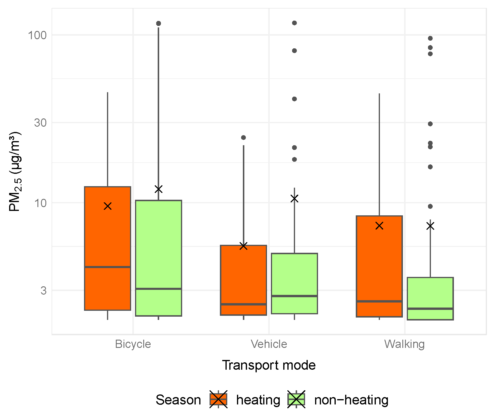
reports general information on the monitoring campaign during heating and non-heating season, including trip time (min) and distance per mode of transport, as well as environmental conditions. Data present average value ± standard deviation. Figure 2 presents box plots of average concentrations of PM_2.5 and NO₂ over a single trip (based on 1-min data from both commuters) by each mode of transport during heating and non-heating seasons.

During the non-heating season, average temperatures range from about 16–19 °C across the three modes, while during the heating season, the temperatures drop considerably (around 8–10 °C), reflecting cooler conditions typical of winter. Atmospheric pressures for bicycle and vehicle travel modes are around 990 hPa, while walking shows more variation. Compared to the non-heating season, the heating season exhibited higher atmospheric pressures (995–998 hPa), which are typical for colder weather conditions. Relative humidity was relatively similar across modes (62–68%) during the non-heating season as well as for bicycles and vehicles (64–65%) during the heating season but showed a notable decrease for walking routes (dropping from nearly 68% to about 57%). Bicycle and vehicle commuters experienced similar wind speeds (1.5–1.6 m/s) during both seasons but increased noticeably for pedestrians (up to about 1.8 m/s) during the heating season.

Mean values of NO₂ and PM_2.5 show statistically significant differences between the heating season and the non-heating seasons (p = 0.025 and 0.032). For NO₂ during the heating season, both the average 30.8 µg/m³ (median 25.6 µg/m³) and the range of concentrations 0.1–109.6 µg/m³ are higher compared to the non-heating season, where the average was 22.6 µg/m³ (median 20.4 µg/m³), and the range was 0.2–103.3 µg/m³. The larger interquartile range in the heating season indicates greater variability in concentrations, meaning that NO₂ levels vary more during this period. For PM_2.5 concentrations, seemingly contradictory results are observed between the measures of central tendency. During the heating season, the mean concentration is 8.1 µg/m³ (median: 3.2 µg/m³), with values ranging from 2.0 to 45.5 µg/m³. During the non-heating season, the mean concentration is 9.9 µg/m³ (median: 2.6 µg/m³), and values range from 2.0 to 117.8 µg/m³, indicating a higher mean concentration compared to the heating season but a lower median concentration. The discrepancy between the mean and median values in the non-heating season suggests greater variability and the presence of outliers, which inflated the mean value. A probable explanation for this observation may relate to short-term local sources (e.g., construction activity, resuspended road dust, or increased vehicular emissions during dry and warmer periods) that are more prevalent in the non-heating season. Furthermore, specific meteorological conditions—such as lower relative humidity and less atmospheric stability in warmer months—may contribute to elevated peak concentrations under certain circumstances. Conversely, while the heating season is typically associated with increased emissions from residential heating, atmospheric conditions such as temperature inversions and reduced vertical mixing can suppress dispersion and lead to more consistently elevated background levels, which may explain the higher median concentrations observed during that period.

3.2. Comparison Across Commuting Modes

The comparison of three commuting modes (by bicycle, vehicle, and walking) during non-heating season revealed that the longest average commuting time was by vehicles (46.5 min) while walking was the shortest (20.7 min). Bicycle commuting time increased in the heating season (+4.2 min), while vehicle use was reduced (−8.8 min). However, these differences were not significantly different (p > 0.05). Analysis of the length of trips indicated that only in the case of bicycle trips was a significant difference between the heating (5.6 km) and non-heating (3.6 km) seasons observed.

Figure 2 and Figure 3 present the direct comparisons between concentrations of NO₂ and PM_2.5 during heating and non-heating seasons for three travel modes based on the average concentration over a single trip. The result of the Kruskal–Wallis test (p = 0.480) showed no statistically significant differences in NO₂ levels between groups (bicycle, vehicle, or walking). During the heating season, the mean concentrations of NO₂ recorded while traveling by bicycle, walking, and by vehicle were 28.1, 33.0, and 34.8 µg/m³, respectively, with the mean concentration increasing in the order: bicycle < walking < vehicle (median values 19.2, 33.1, and 32.8 µg/m³. In contrast, during the non-heating season, the mean concentrations followed the order: walking < bicycle < vehicle, with mean values of 21.4, 22.7, and 24.8 µg/m³, and median values of 20.4, 19.9, and 20.8 µg/m³, respectively. The lack of significant differences indicates that the choice of transport mode is not a determining factor in the NO₂ concentration. In the case of PM_2.5 concentrations, the Kruskal–Wallis test (p < 0.05) showed statistically significant differences between the groups. The highest mean rank was observed for trips made by bicycle, while the lowest was recorded for walking, suggesting that the mode of transport may influence exposure to PM_2.5. Vehicle users did not exhibit significantly different exposure levels compared to the other modes of transport. During the heating season, the mean concentrations of PM₂.₅ increased in the order: vehicle (5.5 µg/m³) < walking (7.3 µg/m³) < bicycle (9.5 µg/m³), with corresponding median values of 2.5, 2.6, and 4.1 µg/m³, respectively. In the non-heating season, the mean concentrations followed the order: walking (7.3 µg/m³) < vehicle (10.6 µg/m³) < bicycle (12.1 µg/m³), with respective median values of 2.3, 2.8, and 3.1 µg/m³. The differences in NO₂ and PM_2.5 concentrations measured by individual sensors were not statistically significant between seasons, contrary to the stationary measurements at the Air lab and monitoring station, which showed statistically significant differences between seasons (p < 0.05). Seasonal trends were evident in the stationary monitoring data but not in the mobile sensor measurements, possibly due to variability in individual exposure patterns while moving. While traveling, personal exposure might be influenced more by local sources (e.g., traffic emissions near the route). Movement and changing surroundings may cause air pollution levels to fluctuate rapidly, making it harder to detect seasonal trends.

In order to examine whether the choice of transport mode varies between the two participants, an additional analysis was conducted, considering the individual as a differentiating factor. The results of the Kruskal–Wallis test showed that person 1 (male participant) traveling from the suburbs to the city center was exposed to significantly different NO₂ levels between modes of transport. The mean ranks indicate that the highest NO₂ values are associated with walking, while the lowest is for cycling, in contrast to person 2 (female participant), who traveled mainly in the city center and did not experience significant differences in exposure between the three modes of transport. On the other hand, for PM_2.5 exposure, significant differences in mode of transport were observed only for person 2 (p = 0.02). A female participant was exposed to higher concentrations of PM_2.5 when cycling or using a vehicle, while her exposure was the lowest while walking. No significant differences were found for person 1 (p = 0.16), suggesting PM_2.5 concentrations were not significantly different between his modes of transport.

3.3. Considering Inhaled Doses Instead of Concentrations

Generally, without distinguishing the mode of transport or season, the mean value of the total inhaled dose of NO₂ was higher for the male (32.8 μg) than the female (23.9 μg), and the difference was not statistically significant (p > 0.05). The median in both was significantly lower than the mean (13.2 μg for the male and 13.3 μg for the female). The maximum values were similar for both participants, but the greater spread of values for the female participant’s dose indicates greater variability in the data. For PM_2.5, the mean value of the total inhaled dose was twice as high for the male participant (16.8 μg) as for the female (8.3 μg); the difference was significant (p = 0.004). The median was also higher in the male (6.6 μg) than in the female participant (1.5 μg) exposure, and the wide range of values for both participants confirms the presence of outliers.

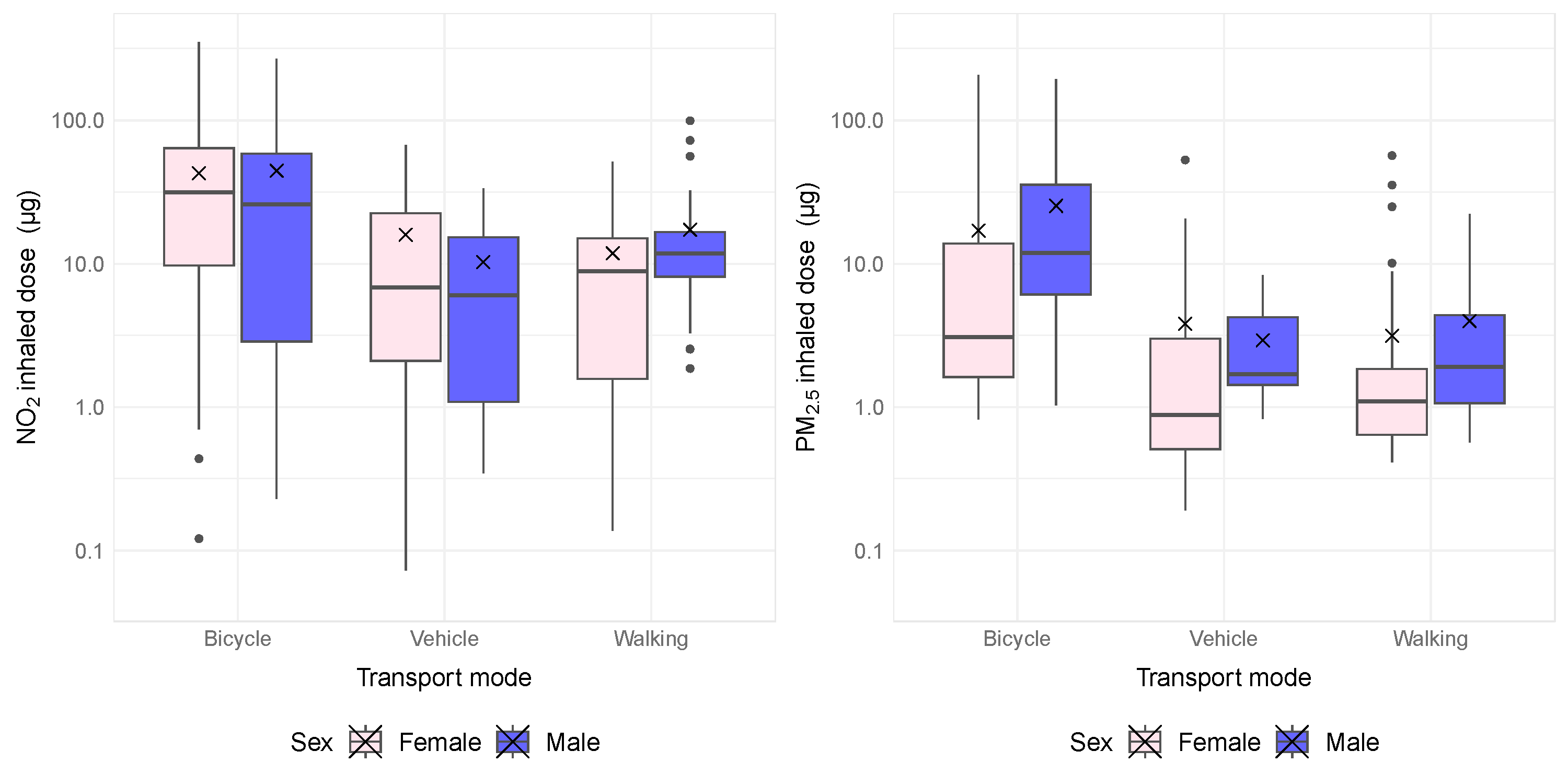
After separating the doses according to the mode of transport and participants (Figure 4) for both pollutants, the bicycle emerged as the mode of transport with the highest inhaled dose per trip. For NO_2, the mean dose inhaled by the male participant was 44.5 μg (median 25.9 μg), while for the female participant, 42.6 μg (median 31.4 μg). For PM_2.5, mean values were 25.3 μg and 17.1 μg (median 11.9 μg and 3.1 μg), respectively, with no statistically significant difference between the participants. In the case of both pollutants, the inhaled dose during cycling was significantly higher than in other modes of transport (p < 0.05), and no statistically significant difference was observed between the dose inhaled during commuting by vehicle and walking. The doses during trips by bike were significantly higher than by vehicle and walking, which is related to higher VR for cycling (MET > 6).

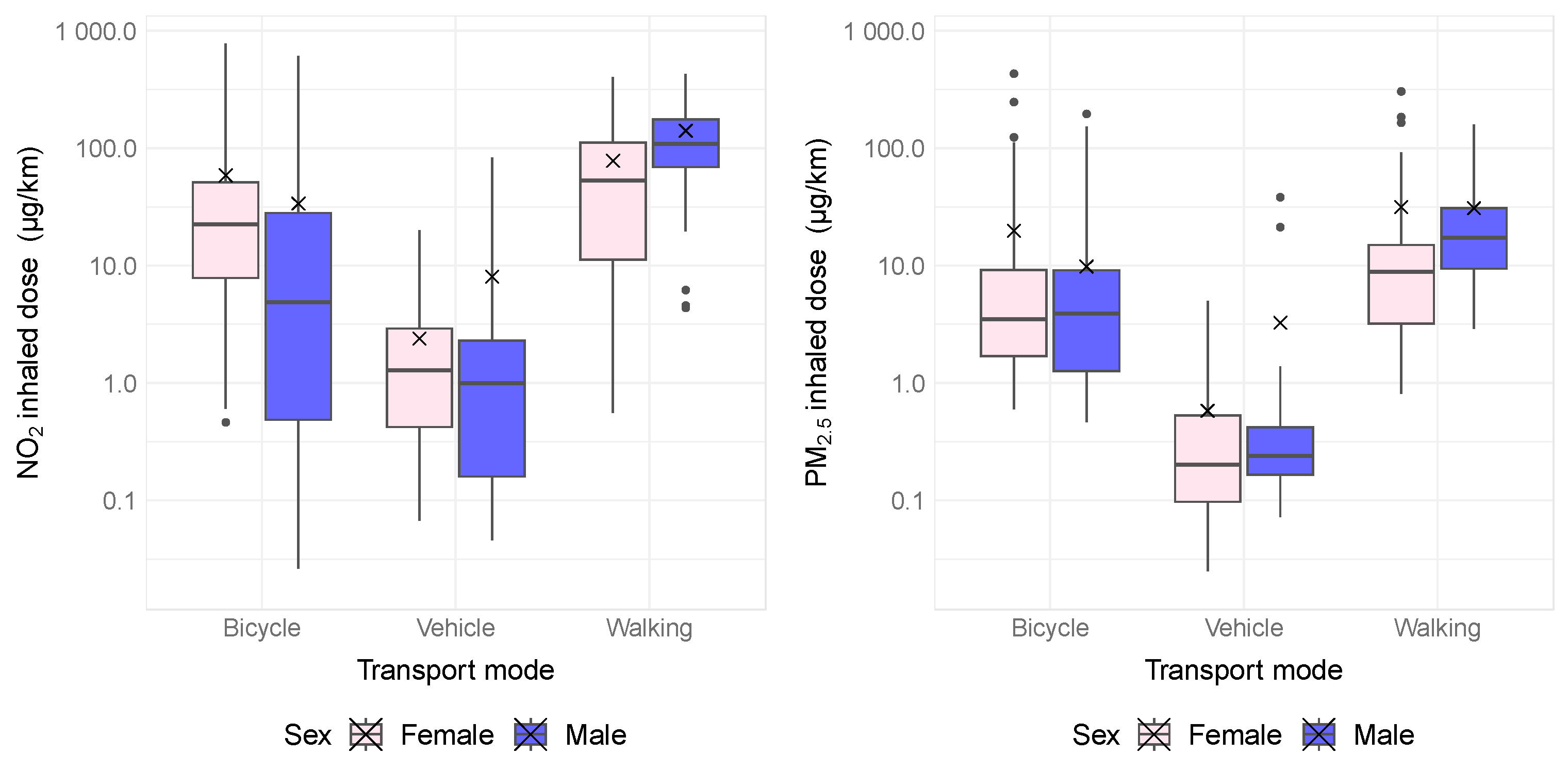
Figure 4 shows the dose of NO₂ and PM_2.5 inhaled by the female participant and the male participant per trip (μg), while Figure 5 presents the inhaled dose per kilometer traveled (μg/km). It can be noted that the trend of inhaled dose per trip differs from the corresponding trend of inhaled dose per km. In the case of both pollutants, if distance is included, the highest dose per kilometer was found during walking. Without distinguishing the mode of transport or season, the mean value of the total inhaled dose of NO₂ was higher for the male (58.3 μg/km, median 8.4 μg/km) than for the female (52.2 μg/km, median 14.9 μg/km). For PM_2.5, the female inhaled higher doses per km, and the mean dose was 19.6 μg/km (median 3.1 μg/km). In comparison, the mean dose for the male participant was 14.4 μg/km (median 4.6 μg/km). The difference between the male participant and the female participant was not statistically significant (p > 0.05). Gender and driving mode analysis points out that the PM_2.5 dose inhaled per km differs significantly between modes of transport (p < 0.05). The highest dose was inhaled while walking, while the lowest dose was for vehicles. The mean dose for NO₂ during walking was 141.3 μg/km (median 109.1 μg/km) and 77.9 μg/km (median 52.9 μg/km) for the male and the female participant, respectively. In comparison, the mean doses for PM_2.5 during walking were 30.8 μg/km (median 17.3 μg/km) and 31.6 μg/km (median 9.2 μg/km) for the male participant and the female participant, respectively. The ranking of inhaled doses per kilometer is as follows: walking > bicycle > vehicle. This reflects the interplay between exposure duration, breathing rate, and pollutant filtration effects. Cycling is a physically demanding activity that increases breathing rate and tidal volume, leading to a higher intake of air—and consequently, pollutants—compared to passive travel in a vehicle. In contrast, vehicle occupants have lower respiratory ventilation rates due to the sedentary nature of car travel. Although cyclists are exposed to ambient air pollutants, they move more quickly through polluted areas than pedestrians, reducing their overall exposure duration in high-pollution areas. Additionally, cyclists tend to travel in dedicated lanes or side roads, which may have lower traffic emissions than pedestrian walkways adjacent to roads with heavy traffic. Unlike vehicles, which offer some degree of air filtration and shielding from direct exposure to exhaust emissions, both cyclists and pedestrians are fully exposed to ambient air pollution. This leads to a higher inhaled dose compared to vehicle occupants.

4. Discussion

The study provided valuable insights into the variability of exposure to air pollutants across different modes of transport during both the heating and non-heating seasons. The analysis of travel patterns, environmental conditions, and pollutant concentrations revealed significant seasonal differences and transport-mode-specific exposure trends to PM_2.5 and NO₂.

Data from fixed air quality monitoring stations indicated that concentrations of both PM_2.5 and NO₂ were higher during the heating season compared to the non-heating season. This finding aligns with previous research and is attributed to increased emissions from residential heating and unfavorable meteorological conditions that limit pollutant dispersion.

In contrast, personal exposure measurements using low-cost sensors, which accounted for transport mode and season, exhibited inverse seasonal trends. This may be explained by the dynamic nature of personal exposure during commuting, where local emission sources and variable traffic conditions play a crucial role. This highlights the necessity of supplementing fixed monitoring data with mobile measurements to achieve a comprehensive assessment of air pollution exposure. Comparing our findings to studies in other regions (

Table 2. Exposure concentration of PM_2.5 and NO₂, as well as the inhaled dose, during three modes of transport: bicycle, vehicle, and walking in different locations.

Mode of Transport	Person	Location	Mean (Min–Max) Concentration Per Trip, µg/m3		Mean (Min–Max) Dose, µg/km		References
			PM2.5	NO2	PM2.5	NO2
Bicycle	Adults	Gliwice	Heating: 9.5 ± 11.1 (2.0–45.5) Non-heating: 12.1 ± 24.0 (2.0–117.2)	Heating: 28.1± 27.7 (0.1–87.8) Non-heating: 22.7 ± 20.3 (0.2–103.3)	Male: 9.8 (0.5–195.7) Female: 19.8 (0.6–431.6)	Male: 33.8 (0.03–610.8) Female: 58.7 (0.5–778.9)	Our results
	Adults	Barcelona, Spain	29±1.7		32.8 * 35.6 per 1 h		[23]
	Children	Hamilton, Canada	15.7±19.3 (10.4–32.3)		2.18 * (0.085–5.67)		[37]
	Adults	Thessaloniki, Greece	55.7		7.9		[38]
	Adults	Montreal, Canada		120.94 (56.13–197.21)		18.73	[39]
	Adults	Xi’an, China	38.6 ± 17.1 (19.0–116.8)		7.4 ± 5.0		[40]
	Adults	Lisbon, Portugal	30.5 ± 9.0 (20.7–61.6)		60		[41]
	Adults	Lisbon, Portugal	8 h: 85 ± 66 11 h: 70 ± 47 14 h: 44 ± 38 17:30 h: 67 ± 43 21 h: 65 ± 26		8 h: 28.01 11 h: 23.81 14 h: 15.38 17:30 h: 25.23 21 h: 13.04		[42]
	Adults	Milan, Italy	Winter: 21.5 Summer: 16.9	Winter: 30.6 Summer: 57.5	5.5 *	12.8 *	[43]
	Adults	Milan, Italy	N/A		Female: Winter: 13.6–107.4 a Summer: 6.2–70.2 a Male: Winter: 9.5–93.9 a Summer: 7.2–81.0 a		[44]
	Adults	Salt Lake City, USA	12.62		1.03		[45]
	Adults	Mexico City	42		10.59		[46]
	Adults	Vellore, India	Morning 101 (61–149) Afternoon 92 (62–122)		12–17		[47]
Vehicle	Adults	Gliwice	Heating: 5.5 ± 6.0 (2.0–24.4) Non-heating: 10.6 ± 23.2 (2.0–117.9)	Heating: 34.7 ± 30.2 (0.3–109.6) Non-heating: 24.8 ± 21.6 (1.0–97.4)	Male: 3.3 (0.07–38.2) Female: 0.6 (0.02–5.0)	Male: 8.1 (0.05–83.7) Female: 2.4 (0.01–20.0)	our results
	Adults	Barcelona, Spain	Bus: 25±1.4 Car: 35 ± 1.3		Bus: 18.0 * 20.0 per 1 h Car: 19.7 * 22.1 per 1 h		[23]
	Adults	Thessaloniki, Greece	Bus: 84.6 Car: 32.9–53.1		Bus: 6.9 Car: 1.7–3.1		[38]
	Adults	Montreal, Canada		Bus: 87.62 (24.49–161.90) Car: 114.87 (45.04–177.45)		5.52 car 6.78 bus	[39]
	Adults	Lisbon, Portugal	Bus: 28.4 ± 5.3 (20.7–61.6) Car: 33.7 ± 8.6 (20.7–61.6)		Bus: 25 Car: 13		[41]
	Adults	Lisbon, Portugal	Bus: 8 h: 56 ± 55 11 h: 30 ± 18 14 h: 52 ± 27 17:30 h: 50 ± 23 21 h: 40 ± 16 Car: 8 h: 61 ± 12 11 h: 55 ± 13 14 h: 52 ± 10 17:30 h: 41 ± 7.0 21 h: 35 ± 6.7		Bus: 8 h: 4.89 11 h: 2.36 14 h: 4.40 17:30 h: 3.15 21 h: 2.42 Car: 8 h: 2.16 11 h: 1.82 14 h: 1.99 17:30 h: 1.83 21 h: 1.08		[42]
	Adults	Milan, Italy	Car: Winter: 8.0 Summer: 5.3	Car: Winter: 5.9 Summer: 17.0	1.6 *	2.5 *	[43]
	Adults	Milan, Italy	N/A		Car Female: Winter: 5.1–66.1 a Summer: 3.8–43.0 a Male: Winter: 6.0–38.1 a Summer: 4.3–53.0 a		[44]
	Adults	Salt Lake City, USA	Bus: 13.03 Car WO: 15.21 Car WC: 5.31		Bus: 0.2 Car WO: 0.46 Car WC: 0.12		[45]
	Adults	Mexico City	Bus: 38 Car: 32 Carsharing: 29.5		Bus: 5.77 Car: 3.09 Carsharing: 2.77		[46]
	Adults	Vellore, India	Bus: morning 118 (96–150) afternoon 111 (89–138) Car: 174 (150–202)		Bus: 3–4 Car: 2–6		[47]
	Adults	Bogotá, Colombia	130.0–176.3		Bus: 460.8 µg/day		[48]
	Adults	Singapore	Bus: 28 ± 6 Taxi: 27 ± 7		Bus: 3.0 * Taxi: 2.4 *		[49]
Walking	Adults	Gliwice	Heating: 7.3 ± 10.0 (2.0–44.7) Non-heating: 7.3 ± 17.0 (2.0–95.4)	Heating: 33.0 ± 23.4 (0.7–78.6) Non-heating: 21.4 ± 15.4 (0.6–59.5)	Male: 30.7 (2.9–159.1) Female: 31.6 (0.8–838.7)	Male: 141.3 (4.4–428.9) Female: 77.9 (0.6–401.4)	our results
	Adults	Barcelona, Spain	21 ± 1.3		35.1 * 36.1 per 1 h		[23]
	Children	Hamilton, Canada	15.7–19.3 (10.4–32.3)		3.21 * (0.13–8.31)		[37]
	Adults	Milan, Italy	Low traffic: Winter: 14.5 Summer: 16.7 High traffic: Winter: 16.9 Summer: 13.6	Low traffic: Winter: 25.5 Summer: 39.9 High traffic: Winter: 39.5 Summer: 37.5	Low traffic: 2.8 * High traffic: 13.0 *	Low traffic: 5.8 * High traffic: 32.9 *	[43]
	Adults	Milan, Italy			Female: Winter: 11.9–121.8 a Summer: 9.2–66.5 a Male: Winter: 13.7–127.0 a Summer: 10.6–76.8 a		[44]
	Adults	Salt Lake City, USA	12.21		2.53		[45]
	Adults	Mexico City	34		10.41		[46]
	Adults	Vellore, India	118 (83–154)		8–21		[47]
	Adults	Bogotá, Colombia	55.6		277.8 µg/day		[48]
	Adults	Singapore	36 ± 9		23.1 *		[49]
	Adults Teens	Xi’an, China	35.4 (10.5–67)		8.65 Adults 6.75 Teens		[50]

*—in µg per trip. ^a—in µg during the trip time from 15 to 90 min. N/A—not available. WO—window closed. WC—window open.

) revealed considerable variations in pollutant exposure.

4.1. Differences in Pollutant Concentrations

Analysis of PM_2.5 and NO₂ concentrations measured by low-cost sensors revealed notable seasonal differences. Our analysis of each mode of transport, obtained from measurements by low-cost sensors, reveals substantial differences between heating and non-heating seasons. For PM_2.5, concentrations during the non-heating season were slightly higher (12.1 ± 24.0 μg/m³) compared to the heating season (9.5 ± 11.1 μg/m³), whereas NO₂ concentrations exhibited an inverse trend, being higher in the heating season (28.1 ± 27.7 μg/m³) than in the non-heating season (22.7 ± 20.3 μg/m³). This suggests that transport emissions during the heating season contribute significantly to NO₂ pollution, whereas PM_2.5 levels might be more influenced by atmospheric conditions.

There is a growing body of research investigating exposure to PM_2.5 in relation to mode of transport; however, a clear knowledge gap remains regarding exposure to nitrogen dioxide (NO₂) in this context (Table 2). For example, in Hamilton, Canada, children cycling experienced a PM_2.5 concentration of 15.7 ± 19.3 μg/m³, while studies in Thessaloniki, Greece, reported a significantly higher PM_2.5 concentration of 55.7 μg/m³. Similar trends are evident in Lisbon, Portugal, where PM_2.5 concentrations ranged between 30.5 ± 9.0 μg/m³ and 85 ± 66 μg/m³, depending on the time of measurement. Furthermore, NO₂ concentrations in Montreal, Canada, were markedly higher (120.94 μg/m³), demonstrating significant geographical discrepancies in exposure levels.

During vehicle trips, PM_2.5 concentrations were also higher in the non-heating season (10.6 ± 23.2 μg/m³) compared to the heating season (5.5 ± 6.0 μg/m³), whereas NO₂ concentrations were higher in the heating season (34.7 ± 30.2 μg/m³) than in the non-heating season (24.8 ± 21.6 μg/m³). Comparing these findings to studies in other cities, significant differences in pollutant exposure are evident. For instance, in Thessaloniki, Greece, PM_2.5 concentrations in buses (84.6 μg/m³) and cars (32.9–53.1 μg/m³) were considerably higher than in Gliwice. Similarly, in Montreal, Canada, PM_2.5 concentrations in buses (87.62 μg/m³) and cars (114.87 μg/m³) were elevated. Lisbon, Portugal, displayed moderate values, with PM_2.5 levels in buses (28.4 ± 5.3 μg/m³) and cars (33.7 ± 8.6 μg/m³). Milan, Italy, exhibited seasonal variations in PM_2.5 levels for car users, with higher winter concentrations (8.0 μg/m³) than summer (5.3 μg/m³), mirroring the trend observed in Gliwice.

Walking during the heating season resulted in an average PM_2.5 concentration of 7.3 ± 10.0 µg/m³, with a range between 2.0 and 44.7 µg/m³, while NO₂ concentrations reached 33.0 ± 23.4 µg/m³, ranging from 0.7 to 78.6 µg/m³. During the non-heating season, PM_2.5 levels remained at 7.3 ± 17.0 µg/m³ (2.0–95.4 µg/m³), while NO₂ levels were lower at 21.4 ± 15.4 µg/m³ (0.6–59.5 µg/m³). This seasonal trend is consistent with the previously observed increases in pollutant levels during colder months due to heating emissions.

4.2. Analysis of Exposure According to Commuting Patterns

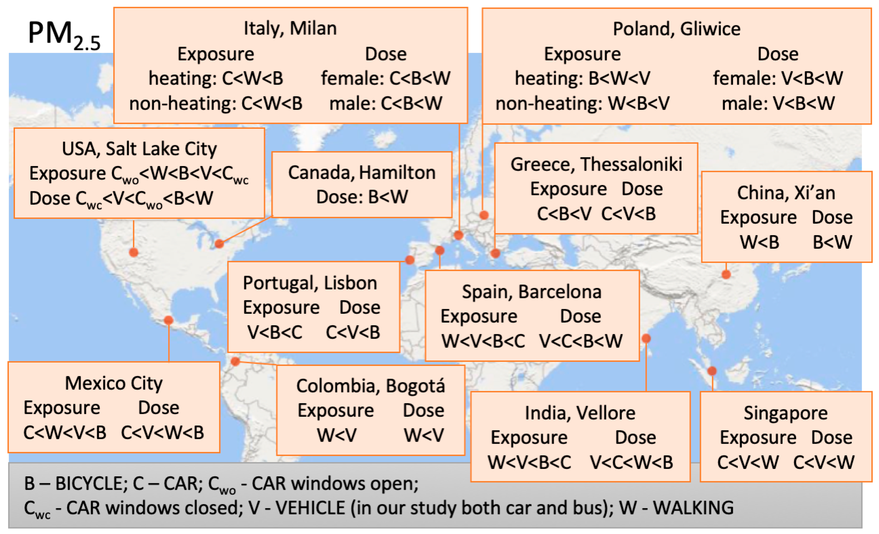
Figure 6 summarizes PM_2.5 exposure associated with different modes of transport across various global cities, highlighting clear spatial and contextual differences. In several locations, such as Salt Lake City (USA), Barcelona (Spain), and Hamilton (Canada), the lowest concentrations were recorded inside private cars with closed windows, while the highest exposures occurred during walking or cycling. In cities like Bogotá (Colombia) and Vellore (India), pedestrians and cyclists experienced the greatest exposure, likely due to direct proximity to traffic emissions. Only in European cities such as Milan (Italy) and during our study in Gliwice was seasonal variation presented—exposure levels were notably higher during the heating season compared to non-heating periods. These examples demonstrate that the mode of transport, local infrastructure, and seasonal factors substantially influence personal exposure to PM_2.5 in urban environments.

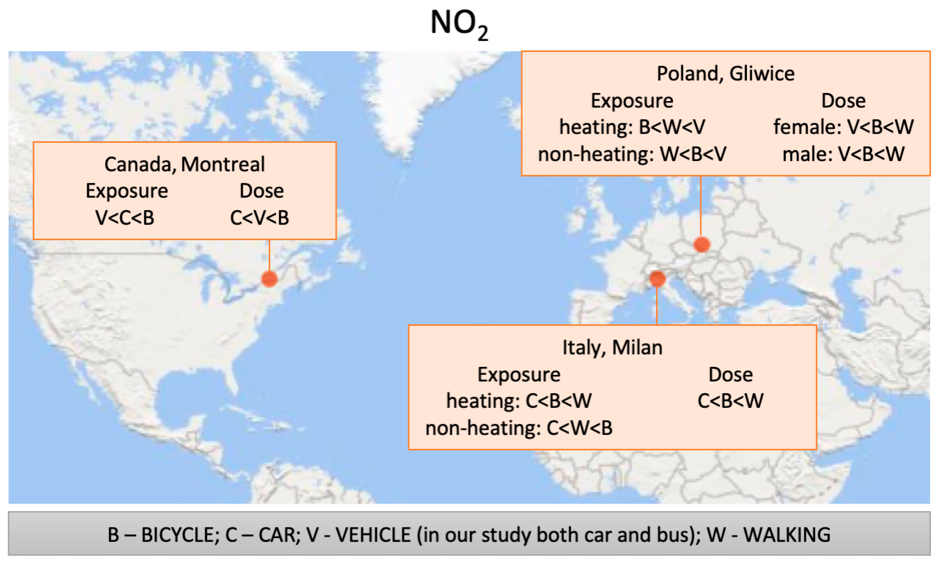
Figure 7 summarizes NO₂ exposure levels associated with different modes of transport in three urban locations: Montreal (Canada), Milan (Italy), and our study in Gliwice (Poland). Across all cases, individuals traveling by vehicle (V) experienced the lowest NO₂ concentrations, while higher exposures were generally observed among those walking (W) or cycling (B). In Montreal, the exposure ranking was V < C < B, suggesting a clear protective effect of enclosed vehicle environments. Similarly, in Milan, exposure during the heating season followed the pattern C < B < W, whereas, in the non-heating period, car use offered the greatest protection (C < W < B). In Gliwice, seasonal differences were again apparent: during the heating season, cyclists were the most exposed (B < W < C), while in the non-heating period, the highest concentrations were observed among pedestrians (W < B < C). These findings emphasize that mode of transport, seasonal conditions, and the degree of physical enclosure significantly affect NO₂ exposure in urban settings, with walking and cycling consistently associated with increased concentrations relative to vehicle travel.

The individual analysis of the participants’ exposure patterns provided additional insights. Person 1 (male participant), commuting from the suburbs to the city center, showed significant variations in NO₂ exposure between transport modes, with the highest levels observed while walking. This could be attributed to prolonged exposure in high-traffic urban environments. Conversely, person 2 (female participant), who mainly traveled within the city center, exhibited no significant NO₂ differences between modes but showed higher PM_2.5 exposure when cycling or using a vehicle. These differences underscore the impact of route characteristics, urban infrastructure, and traffic conditions on personal exposure.

4.3. Inhaled Doses of Pollutants

The variability in air pollution exposure across locations highlights the influence of urban air quality. Cities with high pollutant levels, such as Bogotá, Colombia (130.0–176.3 μg/m³ PM_2.5 in buses), and Vellore, India (118–150 μg/m³ in buses, 174–202 μg/m³ in cars), demonstrate the impact of dense traffic and industrial emissions on inhaled doses. In contrast, cities such as Salt Lake City benefit from cleaner air, leading to lower doses. In this comparison, Gliwice appears to be a city with moderate air quality.

A gender-based analysis of inhaled doses demonstrated a notable disparity. During cycling, inhaled doses per kilometer showed higher mean values for the female than the male participant. The mean PM_2.5 dose per kilometer was 19.8 μg/km for the female compared to 9.8 μg/km for the male participant, while the NO₂ dose per kilometer was 58.7 μg/km for the female participant and 33.8 μg/km for the male participant. Several studies also provide insights into inhaled doses during cycling. In Milan, Italy, the inhaled NO₂ dose varied between 12.8 μg/km in winter and 5.5 μg/km in summer, indicating strong seasonal effects. Similarly, studies in Mexico City and Vellore, India, reported higher inhaled PM_2.5 doses (10.59 μg/km and 12–17 μg/km, respectively), comparable to our results from Gliwice.

During traveling by vehicle, the male participant inhaled higher doses of both PM_2.5 (3.3 μg/km) and NO₂ (8.1 μg/km) than the female (0.6 μg/km and 2.4 μg/km, respectively). In Montreal, Canada, car users inhaled an average of 5.52 μg/km PM_2.5 and 6.78 μg/km for bus users, whereas in Lisbon, bus passengers had a PM_2.5 dose of 25 μg/km and car passengers 13 μg/km. In Mexico City, the inhaled PM_2.5 dose for bus users was 5.77 μg/km, while car and carsharing users had lower doses of 3.09 and 2.77 μg/km, respectively. In Salt Lake City, USA, vehicle users had much lower inhaled doses, ranging from 0.2 μg/km in buses to 0.46 μg/km in cars without air conditioning. In comparison, Montreal car users inhaled an average of 5.52 μg/km of PM_2.5, while bus users inhaled 6.78 μg/km. In Lisbon, bus passengers received a PM_2.5 dose of 25 μg/km, whereas car passengers received a dose of 13 μg/km. In Mexico City, the inhaled PM_2.5 dose for bus users was 5.77 μg/km, while car and carsharing users had lower doses of 3.09 and 2.77 μg/km, respectively. In Salt Lake City, USA, vehicle users had much lower inhaled doses, ranging from 0.2 μg/km in buses to 0.46 μg/km in cars without air conditioning.

In the case of walking as a mode of transport, inhaled doses of both PM_2.5 and NO₂ were significantly higher than for bicycle and vehicle users. In Gliwice, pedestrians inhaled the highest doses of PM_2.5, with the male participant averaging 30.7 μg/km and the female participant 31.6 μg/km. For NO₂, the male participant inhaled 141.3 μg/km, whereas the female participant inhaled 77.9 μg/km. These values indicate that walking exposes individuals to increased air pollution due to longer exposure times and direct contact with ambient pollutants. Comparisons with other cities highlight notable differences in pedestrian exposure. In Xi’an, China, PM_2.5 concentrations for pedestrians reached 35.4 μg/m³, with inhaled doses of 8.65 μg/km for adults and 6.75 μg/km for teenagers. In Milan, Italy, pedestrian exposure varied between high- and low-traffic areas, with PM_2.5 concentrations reaching up to 16.9 μg/m³ in winter for high-traffic zones. Similarly, NO₂ exposure was significantly higher in high-traffic areas (39.5 μg/m³ in winter) than in low-traffic zones (25.5 μg/m³ in winter). These results align with findings from Gliwice, where seasonal and traffic-related differences impact pedestrian exposure levels.

Figure 6 summarizes the estimated inhaled dose of PM_2.5 across different modes of transport in selected urban areas, emphasizing the role of physical activity and ventilation rate in personal exposure. In cities such as Barcelona (Spain) and Xi’an (China), just as in our study in Gliwice, the highest doses were associated with walking or cycling, despite these modes not always corresponding to the highest ambient concentrations. This is likely due to increased respiratory rates during physical activity, which enhance pollutant uptake. In contrast, the lowest doses were generally recorded inside private vehicles with closed windows, as seen in Milan (Italy) and Salt Lake City (USA). In Bogotá (Colombia) and Hamilton (Canada), cycling led to significantly higher doses, further illustrating the influence of exertion on inhaled pollutant load. These findings confirm that, beyond ambient concentrations, individual activity level and transport context are key determinants of the actual dose of PM_2.5 received.

A summary of the inhaled dose of nitrogen dioxide (NO₂) across different modes of transport in selected urban areas—Montreal (Canada), Milan (Italy), and during our study in Gliwice (Figure 7)—reveals a consistent pattern in which active modes of travel, such as walking and cycling, are associated with the highest doses. This is attributed to elevated ventilation rates during physical activity, which increases pollutant uptake regardless of ambient concentration. In Montreal, the dose ranking was C < V < B, indicating that cycling results in the highest dose. In Milan, the pattern remained consistent across seasons, with the lowest dose observed in car users and the highest in pedestrians (C < B < W). In Gliwice, sex-specific differences were noted. For the female, the ranking was V < B < W, whereas for the male, it was V < C < W. These results underline that the actual respiratory burden from NO₂ exposure is strongly influenced by the physiological demands of each transport mode in addition to environmental concentrations.

Our findings emphasize the necessity of tailored air quality policies to reduce exposure for commuters using different transport modes. Measures such as improved ventilation in public transport, traffic management strategies, and the promotion of cleaner vehicle technologies could significantly lower inhalation doses for urban travelers.

Additionally, observed gender-based differences may be attributed to variations in respiratory patterns, lung tidal volumes, and cycling speed, where women might inhale more pollutants due to lower ventilation efficiency or different exposure behaviors. However, the elevated inhaled doses among pedestrians emphasize the need for urban planning strategies to mitigate air pollution exposure. Implementing pedestrian-friendly infrastructure, increasing green spaces, and promoting low-emission zones can effectively reduce inhalation risks for city dwellers. Moreover, increasing public awareness regarding pollution exposure during walking could encourage behavioral changes, such as route selection to avoid highly polluted areas.

4.4. Limitations of the Presented Approach

Despite careful planning and execution, this study has several important limitations that must be considered when interpreting the results. The analysis was based on data collected from two individuals, which limits the generalizability of the results to a broader population. Individual differences in routes, pace of movement, and physiology of the participants may have influenced the results. Due to different starting locations and different urban conditions (city center vs. suburban areas), exposure to pollutants may have differed significantly, complicating direct comparability between participants.

The study adopted standard values of minute ventilation rates (VR) corresponding to different modes of transportation without direct measurement of individual exercise, which may have affected estimates of inhaled pollutant doses. The study was conducted over a period of 11 months; thus, the results reflect conditions specific to the year 2022 in Gliwice, which may vary at other times due to changing emission trends and meteorological conditions. In addition, Gliwice, as a city with high levels of air pollution, may not be representative of localities with better air quality or other urban characteristics, thus limiting the ability to extrapolate conclusions to other locations.

4.5. Future Research Needs

In view of these limitations, further research is advisable to deepen and consolidate the results obtained. In particular, it is recommended that the number of participants be increased. Including a larger and more diverse group of people—representing different age groups, genders, physical activity levels, and varied travel routes—would increase the generalizability of the results. It would also be important to include measurements of actual ventilation rates (e.g., using portable spirometers), which would allow more precise estimates of inhaled pollutant doses.

Conducting similar studies in cities with different pollution levels and urban structures would allow comparison and evaluation of the impact of local conditions on exposure. It would also be beneficial to carry out measurements over a number of years to allow analysis of time trends and assessment of the impact of environmental policies on reducing exposure to air pollution.

In addition, future studies could examine the effects of protective measures such as the use of face masks, travel route modifications (e.g., avoiding highly congested streets), or the use of vehicles equipped with advanced air filtration systems on actual exposure levels. Nevertheless, according to the authors, the most recommended approach would be to verify the results using more precise instruments (e.g., reference-grade equipment) under real-world conditions to assess the accuracy of low-cost sensors in individual exposure studies.

5. Conclusions

Cycling was found to offer a balanced trade-off between exposure and inhaled dose. While cyclists were exposed to higher pollutant concentrations than car users, their overall inhaled dose was often lower due to reduced travel duration and lower respiratory intake compared to pedestrians. However, in cities with severe air pollution, cycling may still pose health risks, necessitating protective measures such as improved cycling infrastructure and pollution-reducing interventions.

Vehicle users benefit from enclosed environments, which may reduce pollutant exposure in well-ventilated or air-conditioned cars. However, in areas with high background pollution, vehicle users still experienced notable inhaled doses. Seasonal differences in Gliwice indicated that winter heating played a crucial role in NO₂ levels, whereas PM_2.5 exposure was more influenced by traffic conditions.

Pedestrians experienced the highest inhaled doses of pollutants due to prolonged exposure and physical exertion. This underscores the need for improved urban planning, such as green corridors and traffic-free zones, to minimize pedestrian exposure to harmful air pollutants.

Overall, the findings highlight the importance of urban air quality management and transportation policies to mitigate air pollution exposure for different commuters. Strategies such as promoting cleaner transport technologies, enhancing public transport efficiency, and expanding green urban spaces can play a vital role in reducing health risks associated with air pollution exposure.