1. Introduction
Nowadays, underwater activities are becoming more and more important. These underwater activities include sea exploration, underwater surveillance, monitoring, rescue, etc. Communication in underwater environments is crucial. One communication approach is to use electrical or optical cables; however, their transmission distance and flexibility are limited. Another approach is to use wireless communication via radio-frequency (RF) transmission [
1]; however, radio waves have high attenuation during transmission through water. Acoustic waves can also be used in underwater communication, and they have a much lower absorption than RF transmission in water [
2]. However, acoustic communication has limited transmission bandwidth and high latency [
3]. In order to provide communication between autonomous underwater vehicles (AUVs), divers or sensor nodes, visible light communication (VLC) [
4,
5,
6,
7,
8,
9,
10] can be used to provide underwater wireless optical communication (UWOC). VLC is one implementation of optical wireless communication (OWC) [
11,
12] using the visible optical spectrum to carry data, and it is also considered as a potential candidate for future 6G networks [
13,
14]. UWOC can provide high-bandwidth and high-flexibility underwater communication [
15,
16,
17,
18,
19].
Apart from communication under water, direct communication between the water–air interface is also highly desirable [
20,
21,
22,
23]. Air-to-water wireless transmission is crucial for sending control information or instructions from unmanned aerial vehicles (UAVs) or ground stations above the sea surface to AUVs. On the other hand, water-to-air wireless transmission is also required to transmit real-time information from AUVs or sensor nodes to UAVs above the water surface. This scenario is illustrated in
Figure 1, in which communications between UAVs and AUVs across the water–air interface is implemented by VLC. As VLC also supports wide fields-of-view (FOV), several AUVs can receive signals from a single UAV. The system also supports network scalability. The data received by a UAV can be repeated and retransmitted to neighbor UAVs, which in turn retransmit to ground stations via VLC, infrared (IR) or RF links.
Although water–air communication offers many advantages, water–air VLC transmission presents many challenges, such as water absorption and turbulence. Previously, we successfully demonstrated a water-to-air optical camera-based OWC system [
23], which is also known as optical camera communication (OCC) [
24,
25]; however, the reverse transmission (i.e., air-to-water) using OCC has not been analyzed. It is worth noting that for the prior water-to-air OCC system, since the camera is located in the air, the image of the light source would be magnified due to diffraction. Hence, the pixel-per-symbol (PPS) decoding in the OCC pattern would be easier. In the proposed air-to-water OCC system reported here, since the camera is located in the water, the image of the light source in the air will be diminished due to diffraction. Hence, the PPS decoding in the OCC pattern will be more difficult. According to our analysis, when viewing a light source in water from air (i.e., the prior water-to-air OCC system), assuming the distance between the light source and the water–air interface is
h, the light source image appears shallower by ~0.75
h and magnified. However, when viewing the light source in air from water (i.e., the present air-to-water OCC system), also assuming the distance between the light source and the water–air interface is
h, the light source image appears further away by ~1.33
h and diminished. For the OCC system, the distance would affect PPS decoding. From previous experience, the lower the PPS is, the worse the decoding performance becomes. For the present proposed air-to-water OCC system, due to the diminution by distance of the image of the light source, it will be subject to more stringent limitations, and image blurring and distortion will be more severe, presenting more challenges for OCC decoding.
In the case of water–air interface transmission, a wide FOV is required to eliminate the need for active alignment between the optical transmitter (Tx) and optical receiver (Rx). OCC can make use of the large photo-sensitive area of complementary-metal-oxide-semiconductor (CMOS) image sensors for receiving optical signals. Hence, it can provide a wide FOV for detection [
26]. In order to increase the data rate of OCC systems to above the frame rate, the rolling shutter (RS) effect in CMOS can be employed [
27,
28]. Recently, artificial intelligence/machine learning (AI/ML) has been utilized to enhance the decoding performance of the RS pattern, such as convolutional neural networks (CNN) [
29], pixel-per-symbol labeling neural networks (PPSNN) [
30], and long short term memory neural networks (LSTMNN) [
23].
In this work, we propose and experimentally demonstrate a wide FOV air-to-water OCC system using CUDA Deep-Neural-Network Long-Short-Term-Memory (CuDNNLSTM). Due to the effects of water turbulence and air turbulence on AUV and UAV, a precise line-of-sight (LOS) between the AUV and the UAV is difficult to achieve. Here, OCC can provide large FOV for transmission and detection without the need for precise alignment. The CUDA Deep-Neural-Network (CuDNN) is a library of graphics processing unit (GPU)-accelerated primitives designed for deep neural networks. It can speed up the training and inference procedures for deep learning problems. It can also support many neural network designs, such as LSTMNN and CNN. Similar to LSTMNN [
31], the CuDNNLSTM processes memory characteristics to enhance the decoding of OCC signals. Experimental results show that the proposed air-to-water OCC system can support 7.2 kbit/s transmission through a still water surface, and 6.6 kbit/s transmission through a wavy water surface; this performance satisfies the hard-decision forward error correction (HD-FEC) bit-error-rate (BER) of 3.8 × 10
−3. Here, we also compare the proposed CuDNNLSTM algorithm with the PPSNN, illustrating that the CuDNNLSTM algorithm outperforms the PPSNN. Here, we also discuss in detail the implementation of the CuDNNLSTM, as well as the loss and accuracy over time. In addition, we also compare the model training times needed when using CuDNNLSTM and LSTMNN running in Python (version: 3.11.7) on the same computer. The time required for CuDNNLSTM is about eight times less than that required by LSTMNN.
The paper is organized as follows: An introduction and background are provided in
Section 1. The proof-of-concept water-to-air OCC experiment and the CuDNNLSTM algorithm are presented in
Section 2. Then, the results and discussion are given in
Section 3. Finally, a conclusion to summarize this work is provided in
Section 4.
2. Proof-of-Concept Experiment and Algorithm
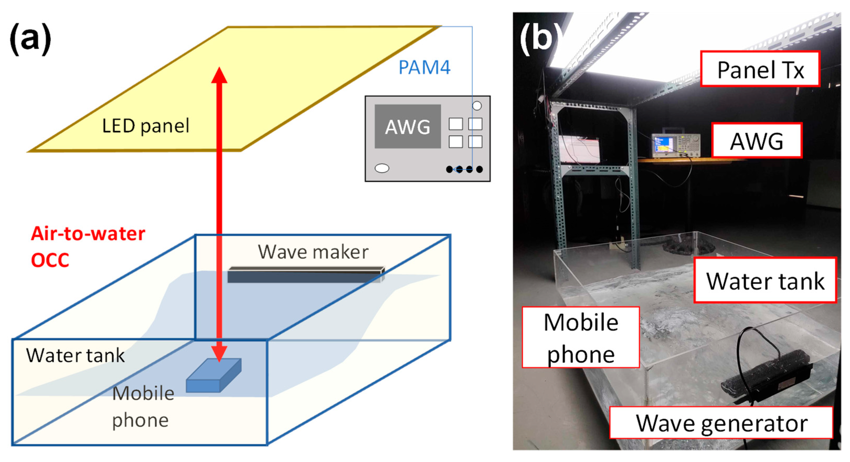
Figure 2a shows the experimental setup of the wide FOV air-to-water OCC system using CuDNNLSTM with light emitting diode (LED) panel Tx and mobile phone CMOS camera for underwater Rx. The authors of [
32] discussed optical Tx designs for maintaining signal integrity, and the authors of [
33] discussed sensor performance under dynamic conditions. The mobile phone used in the experiment was an Asus
® Zenfone
® 3, having 16 MP, resolution of 1920 × 1440 pixels, frame rate of 30 frames per second (fps) and shutter speed of 1/10,000. The mobile phone was placed inside a waterproof transparent case, and immersed in the water to a depth of about 30 cm. The LED panel Tx is connected to an arbitrary waveform generator (AWG) to produce an optical four-level pulse-amplitude-modulation (PAM4) signal. The LED panel was 58 cm × 88 cm in size, and was obtained from Li-Cheng Corp.
® (Taiwan, China). It consists of 108 white-light LED chips, each operating at 0.2 W. As a result, its total power consumption is 21.6 W. The authors of [
34] also discussed other optical modulation techniques in turbulent aquatic environments. The distance between the LED panel and the mobile phone was 100 and 180 cm. A wave generator (Jebao
® SCP-120) was used to produce water turbulence on the surface. The wave generator can only produce a single frequency of 2.8 Hz and a water ripple amplitude of 17%. As illustrated in [
23], the water ripple amplitude percentage is defined as
, where
hpeak is the peak water height and
have is the average water level.
Figure 2b shows a photograph of the experiment: the LED panel Tx is mounted on a metal rack, and below is the water tank with the mobile phone and wave generator.
During RS operation, the CMOS image sensor captures the optical signal row-by-row [
29,
30]. As shown in
Figure 3, if the LED Tx is modulated higher than the frame rate, bright and dark fringes representing Tx “ON” and “OFF” can be observed in the received RS pattern. RS operation allows the OCC data rate (>kbit/s) to be significantly higher than the frame rate (30/60 fps). Although RS operation can significantly enhance the data rate, decoding the data of the RS pattern may create ambiguity. During RS operation, the optical exposure of the subsequent pixel row will start before the exposure completion of the previous pixel row; hence, when the LED Tx is modulated at a high data rate, ambiguity occurs due to the uneven integration of light in the pixel row, as illustrated on the right-hand side of
Figure 3. We can observe that the brightest fringe represents logic 1, and the darkest fringe represents logic 0. However, in some fringes, since the LED Tx “ON” state occurs during part of the exposure time, a gray fringe will result, making it unclear whether it is logic value 1 or 0. This issue will be even more crucial when a PAM4 signal is transmitted. In this work, we employ CuDNNLSTM to enhance PAM4 OCC decoding.
RS decoding is divided into training and testing stages using different received image frames. The training and testing frames number 50 and 318, respectively. A training data set of 50 frames is used for each BER measurement point. Hence, in each BER curve reported later, 500 frames will be used for the training data set. In this data set, 80% is used for training and 20% for validation. Each image frame will be processed in the image and data process module as shown in
Figure 4. First of all, grayscale conversion is performed on each image frame so that each pixel has a value between 0 and 255, irrespective of color. After grayscale value conversion, each pixel row will be arranged according to their grayscale values; hence, the blurred grayscale values due to water ripple and air bubbles can be arranged so that they will not be selected in the subsequent column matrix selection. In column matrix selection, grayscale values between 80% and 90% of the largest value are selected. The reason for the 80–90% threshold is explained as follows: Since we have rearranged the data according to the grayscale value (i.e., brightness) of each pixel in each individual row, the far right and far left values represent the highest brightness and lowest brightness, respectively. We know that overexposed or excessively bright pixels will be placed at the far right, and overly dark pixels, due to uneven brightness distribution, will be placed at the far left. The 80–90% threshold range was determined empirically after multiple trials, which consistently showed that this range best preserves the intended brightness distribution. Hence, those grayscale value columns which are too dark/bright for identifying all four levels of PAM4 signal can be removed. After column matrix selection, the payload and header will be identified. Then, pixel per symbol (PPS) and re-sampling rate are calculated to make sure the same number of pixels is used in each logic symbol for the CuDNNLSTM label. Here, one-hot encoding is performed. The GPU used was an Nvidia
® GeForce RTX3050.
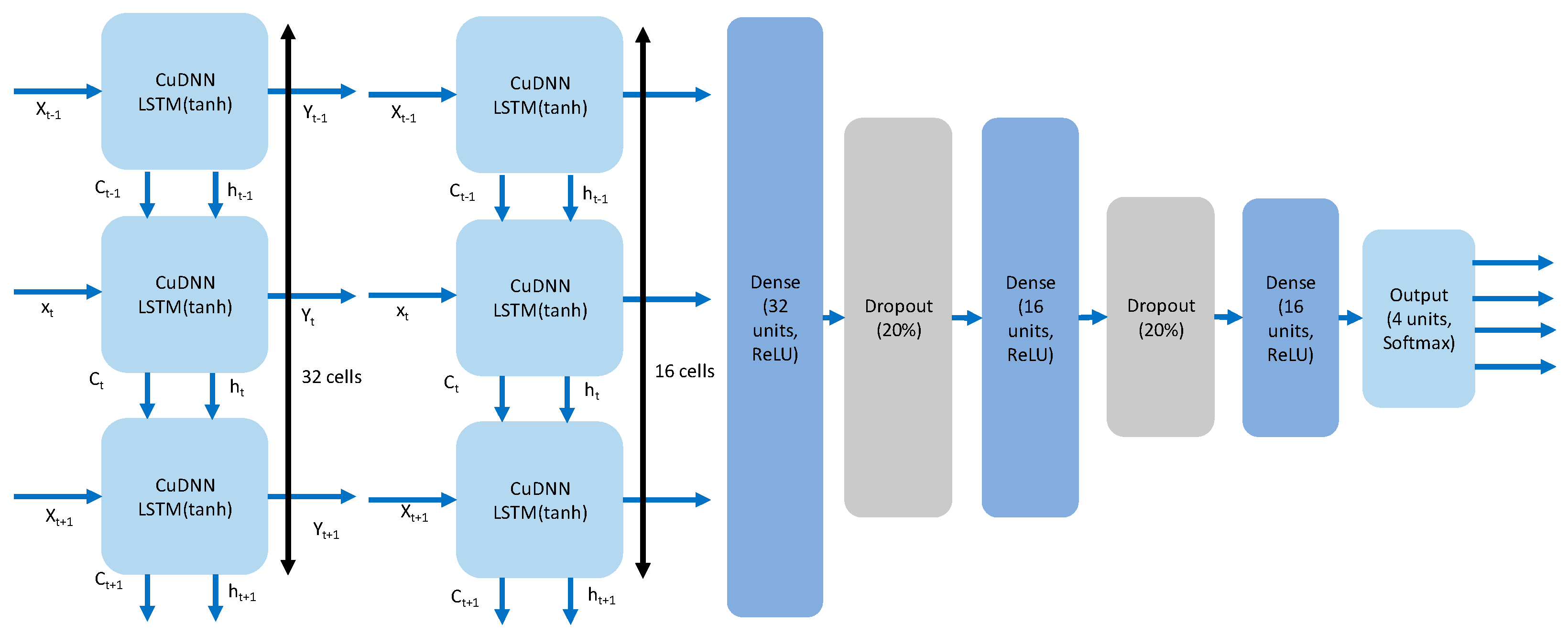
The details of the CuDNNLSTM model are shown in
Figure 5. The CuDNNLSTM model consists of two CuDNNLSTM layers working within the GPU, producing better runtime performance and accuracy. As shown in
Figure 5, the numbers of neuron cells used in the two CuDNNLSTM layers are 32 and 16, respectively. After this, three fully-connected dense layers are used. These three fully-connected dense layers have 32, 16 and 16 neuron cells, respectively. There are two dropout layers to prevent overfitting after the first two fully-connected dense layers. Finally, an output layer obtains the output probabilities of the four levels in the PAM4 signal. The activation function and loss function are ReLU and categorical cross entropy, respectively. The optimizer is Adam for updating parameters. Softmax is used at the output layer to predict the four different logic probabilities.
Figure 5 also shows the CuDNNLSTM cell in the first two CuDNNLSTM layers. The detail of the CuDNNLSTM cell can be found in [
31]. There are several parameters used in the CuDNNLSTM cell:
xt, xt−1, xt+1, ht, ht−1, ht+1, representing the current input, input of last time-step, input of next time-step, hidden state of current cell, hidden state of previous cell, and hidden state of the next cell, respectively. There are three gates in each CuDNNLSTM cell, namely forget gate, memory gate, and output gate. The forget gate decides what kind of information is to be erased, while the memory gate determines what kind of new information to memorize. The output gate generates outputs based on the CuDNNLSTM cell state after different operations.
Equation (1) is the forget gate operation, where
W and
B are the weight and base, respectively. σ is the sigmoid activation function.
Equation (2) is the memory gate operation.
Equations (3) and (4) are the temporary and the current cell state operations, respectively.
As shown in Equation (4), the current cell state can be obtained from the forget gate and the memory gate by multiplying the cell state in its last time-step by the temporary cell state. Equations (5) and (6) are the output gate and hidden state operations, respectively. We can observe that the hidden state is related to the results from the current output gate obtained in Equation (5) and the current cell state from Equation (4).
3. Results and Discussion
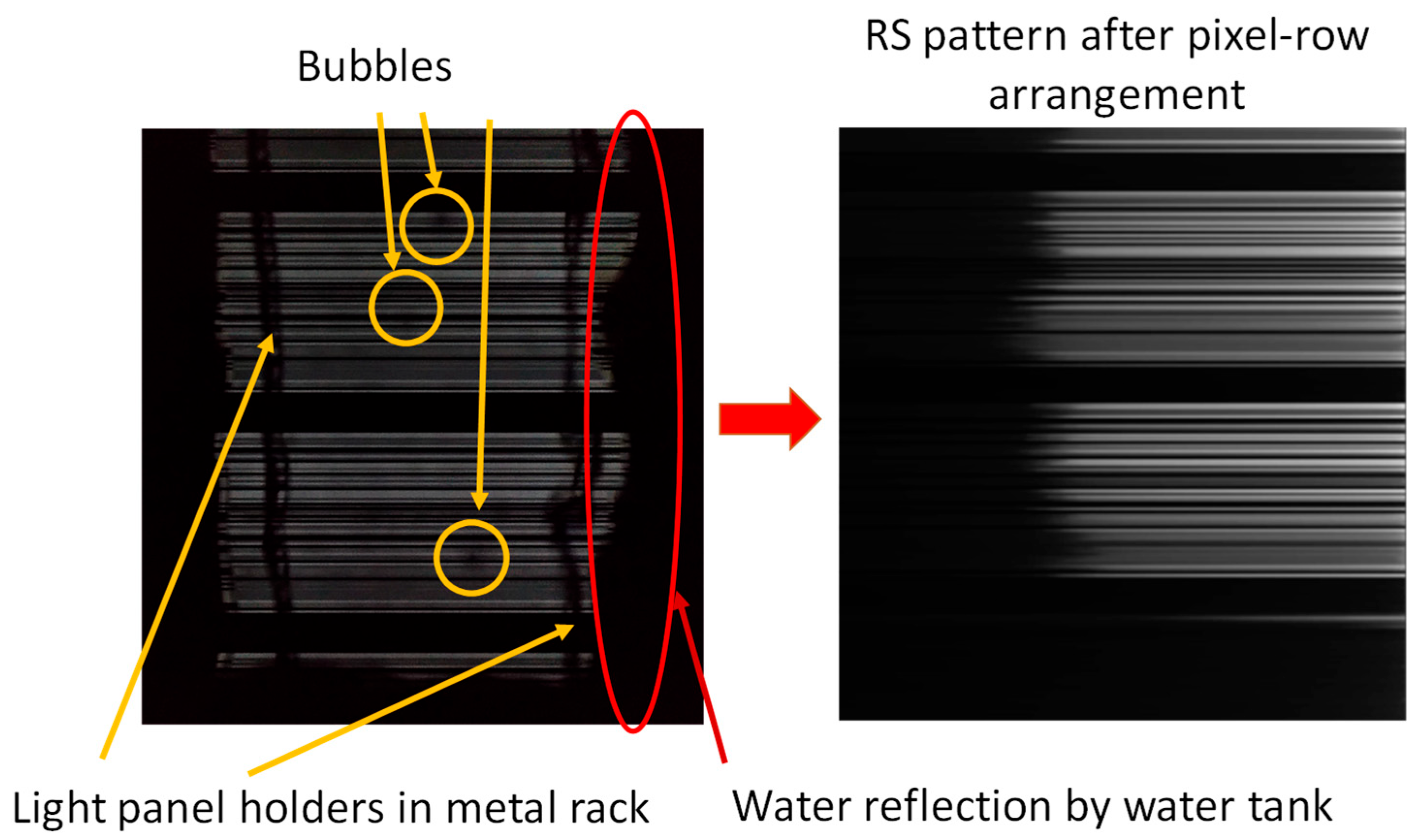
Figure 6 shows the results of the pixel row arrangement in the image and data processing model shown in
Figure 4, in which each pixel row in the obtained RS pattern will be arranged according to their grayscale value. Hence, the grayscale value of each pixel in a row will be arranged in descending order. This means the highest grayscale value in a row will be arranged at the right-hand side, while the lowest grayscale value in a row will be arranged at the left-hand side, as shown in the left-hand figures of
Figure 6. As a result, we can observe that the blurred grayscale values due to water ripples, air bubbles and water tank reflections will be arranged to the left-hand side and they will not be selected in the subsequent column matrix selection. This means that in our experimental environment, we encounter many obstacles (such as the support racks, water bubbles, etc.), and the received images are often degraded. The rearrangement algorithm helps to address these issues.
Figure 6 shows the image after rearrangement, ensuring that decoding is not affected by these obstacles.
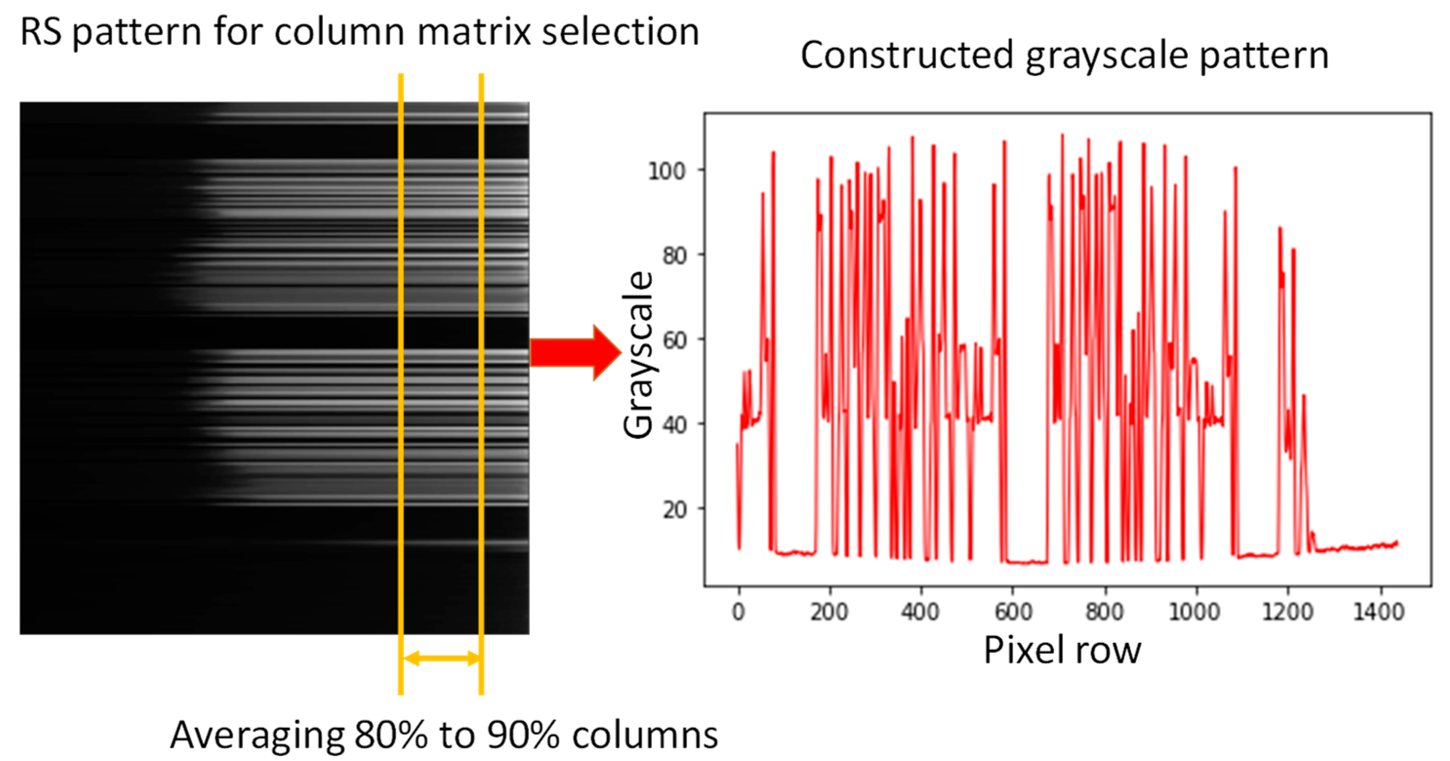
After pixel row arrangement, a column matrix selection based on 80% to 90% of the grayscale value is performed, as shown in
Figure 7. It removes grayscale value columns which are too dark/bright to identify all four levels of the PAM4 signal. Then, a PAM4 data pattern can be obtained as shown on the left side of
Figure 7. We can observe in the constructed grayscale pattern on the left side of
Figure 7 that high amplitude ripples are still observed. Hence, a proper thresholding scheme is needed to identify the PAM4 logic values of 00, 01, 10 and 11. Here, machine learning CuDNNLSTM is utilized for PAM4 logic prediction and identification.
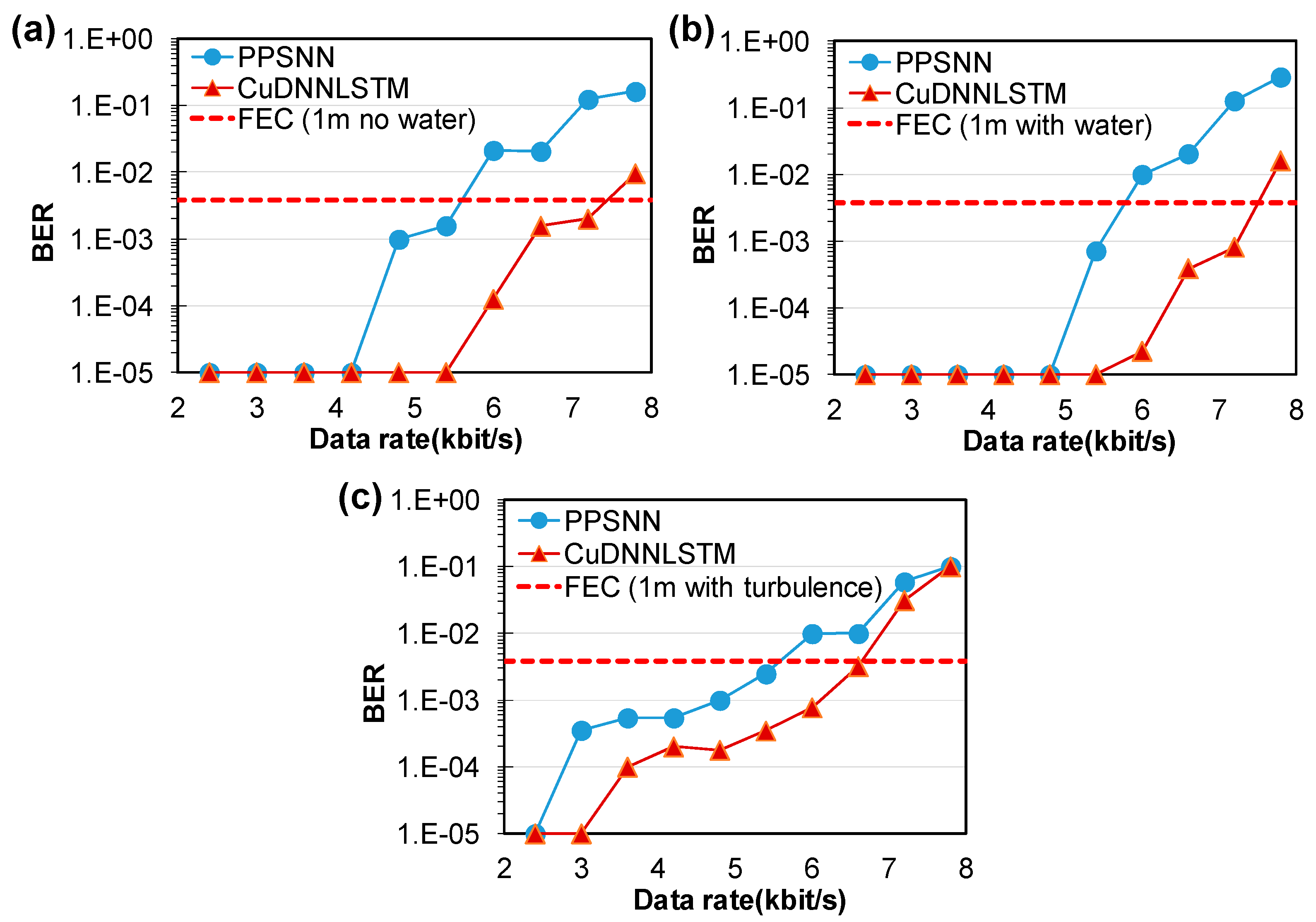
We evaluated the BER performance of the air-to-water RS OCC system using CuDNNLSTM.
Figure 8a–c show the measured BER curves of the air-to-water OCC system under different transmission scenarios. We also compared the proposed CuDNNLSTM algorithm with the PPSNN [
24]. In the no-water case, when the transmission distance was 100 cm, CuDNNLSTM achieved 7.2 kbit/s, satisfying the HD-FEC BER of 3.8 × 10
−3, while the PPSNN only achieved 6 kbit/s. When 30 cm of water is added into the water tank, CuDNNLSTM still achieved 7.2 kbit/s, satisfying HD-FEC, while the PPSNN only achieved 5.4 kbit/s. When water turbulence was introduced, the BER performance of the OCC system becomes higher, and the proposed CuDNNLSTM algorithm still achieved 6.6 kbit/s, satisfying HD-FEC. Here, we first used a preprocessing method to extract signals from the image, and then applied the CuDNNLSTM model for decoding. CuDNNLSTM was primarily used to classify and decode each bit of the PAM4 signal. Compared to other models, it has the advantages of faster speed and lower memory usage, allowing it to be executed on local devices. In this work, the proposed CuDNNLSTM model outperformed the PPSNN model in decoding OCC signals. Here, the use of CuDNNLSTM was combined with one-hot encoding [
35], which can address the more complex temporal characteristics of PAM4 signals. This allowed the model to better learn the relationship between bits at adjacent time points (i.e., depending on parameters we set), while discarding less important information within the same bit. This means that one-hot encoding can help to better distinguish the differences between levels 2 and 3 in PAM4 data. Due to these characteristics, the model can well respond to changes in environmental parameters and provide better decoding performance.
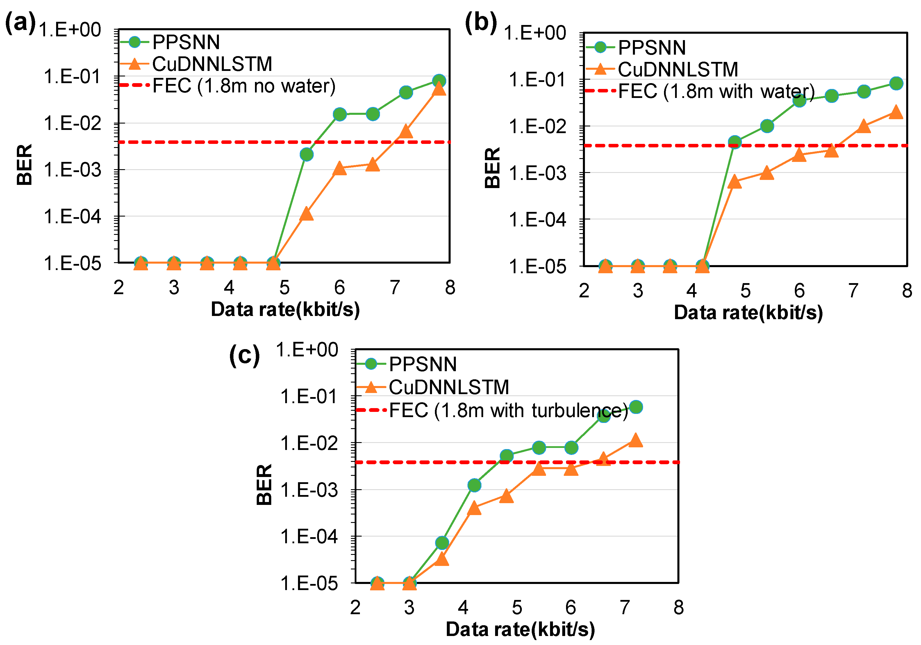
Next, we evaluated the BER performance of the air-to-water RS OCC system when the transmission distance was increased to 180 cm.
Figure 9a–c show the measured BER curves of the air-to-water OCC system under different transmission scenarios. In the no-water case, CuDNNLSTM achieved 6.6 kbit/s, satisfying HD-FEC, while the PPSNN only achieved 5.4 kbit/s. When water was added into the water tank, CuDNNLSTM still achieved 6.6 kbit/s, satisfying the HD-FEC, while the PPSNN only achieved 4.2 kbit/s. When water turbulence was introduced, the BER performance of the OCC system became higher. The proposed CuDNNLSTM algorithm still achieved 6 kbit/s, satisfying the HD-FEC. We also compared the model training times needed when using CuDNNLSTM and LSTMNN running in Python on the same computer. The time required for CuDNNLSTM was 264.89 s, while that for LSTMNN was 2120.13 s (~eight times larger). The laptop computer used was an ASUS
® TUF Gaming A17 FA706ICB with Nvidia
® GeForce RTX3050 GPU GDDR6@4GB (128 bits), CPU: AMD
® Ryzen 5 4600H, RAM: 16 GB.
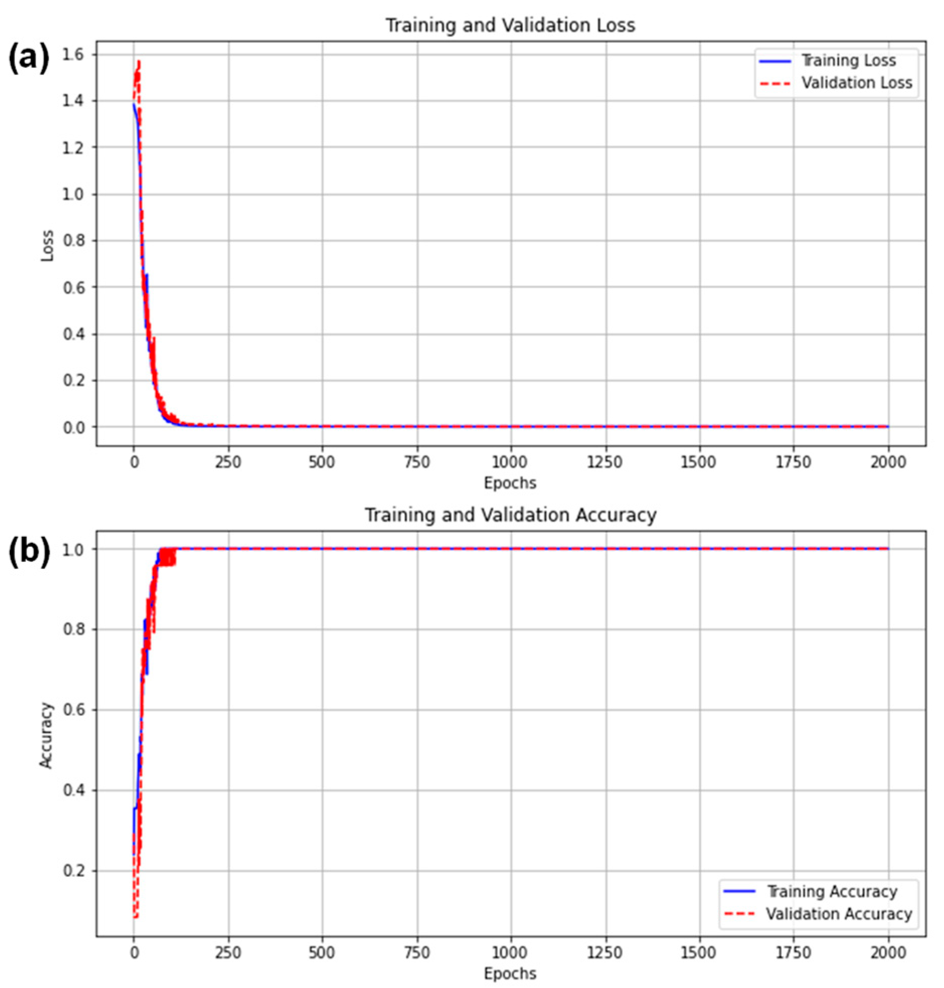
Finally, we evaluated the stability of our trained CuDNNLSTM model.
Figure 10a,b show the measured loss and accuracy over time when using the CuDNNLSTM at a data rate of 7.2 kbit/s under 100 cm transmission distance through wavy water. We can observe in
Figure 10a that the losses of the training and validation data are a good match with each other. The losses decrease rapidly after a few epochs, and become nearly zero after 200 epochs. It is also worth mentioning that when CuDNNLSTM was used, the processing latency was significantly reduced when compared with the traditional LSTMNN model. Hence, the valuation to 2000 epochs can be completed within several minutes. Similarly, as shown in
Figure 10b, the accuracies of training and validation data are a good match with each other. The accuracies increase rapidly after a few epochs, and become nearly 100% after 200 epochs. It is worth noting that CuDNNLSTM is optimized for GPU performance, supporting only Tanh and Sigmoid activation functions, which limits flexibility compared to typical LSTM. The advantage of CuDNNLSTM is that it is more memory-efficient than typical LSTM, as it uses optimized memory allocation for faster computation in the GPU. Other self-defined structures are basically the same as the basic LSTM model.
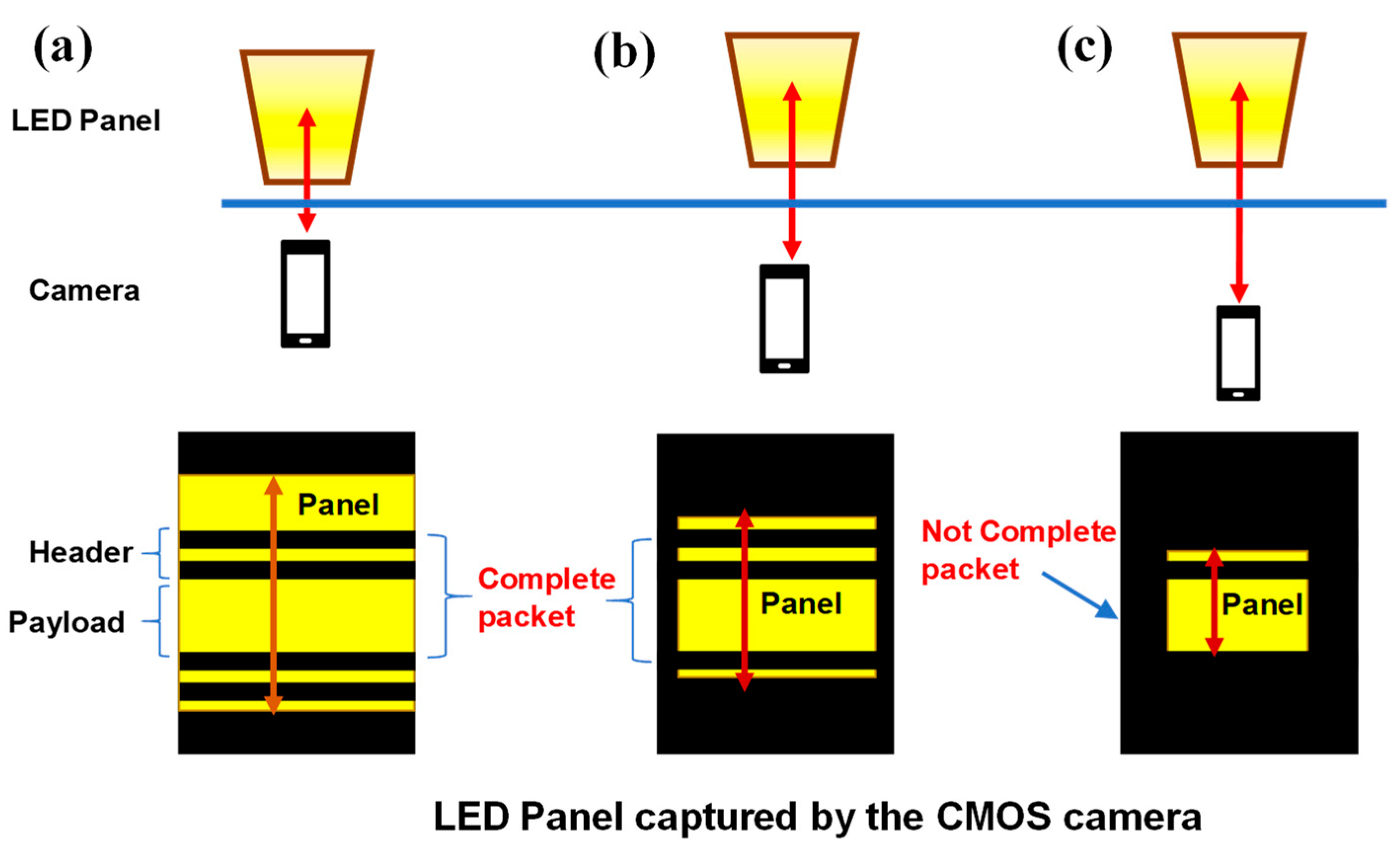
Here, we provide an analysis of the variation in performance when the distance between the LED panel and the CMOS camera changes. As shown in
Figure 11a–c, when the distance between the LED panel and the CMOS camera increases, the LED panel captured by the CMOS sensor becomes smaller and smaller. Since the RS effect is produced by the CMOS camera, increasing the distance will not affect the RS pattern’s bright and dark stripe pixel-widths captured in the CMOS sensor, but it will affect whether a complete OCC packet can be received or not. When the distance is not long, as shown in
Figure 11a, several complete OCC packets (i.e., including a packet header and a packet payload) can be observed. When the distance is very long, as shown in
Figure 11c, a complete OCC packet cannot be observed; hence, data decoding cannot be performed. In order to receive a complete OCC packet over a long transmission distance, the OCC data rate should be decreased; this, in turn, increases the pixel-per-symbol (PPS) value for better RS decoding.
4. Conclusions
Underwater activities are becoming more and more important. As the number of underwater sensing devices grows rapidly, the amount of bandwidth needed also increases very quickly. Apart from underwater communication, direct communication across the water–air interface is also highly desirable. In this scenario, communications between UAVs and AUVs across the water–interface can be implemented by VLC or OCC. As the OCC supports wide FOV, several AUVs can receive signals from a UAV. The data received by the UAV can be repeated and retransmitted to neighbor UAVs, which in turn retransmit to ground stations via VLC, IR or RF links. Previously, we successfully demonstrated water-to-air OCC. However, the reverse transmission (i.e., air-to-water) using OCC had not been analyzed. In this work, we proposed and experimentally demonstrated a wide FOV air-to-water OCC system using CuDNNLSTM, which is a library of GPU-accelerated primitives designed for deep neural networks for speeding up the training and inference procedures. It is worth mentioning that in this proof-of-concept experiment, the controlled water tank neglects some effects of real-life open-water situations, such as sunlight interference, biofouling, or multi-path fading. We used tap water, not salt water. Experimental results showed that the proposed air-to-water OCC system can support 7.2 kbit/s transmission through a still water surface, and 6.6 kbit/s transmission through a wavy water surface; this performance fulfills the HD-FEC BER of 3.8 × 10⁻³. We also compared the proposed CuDNNLSTM algorithm with the PPSNN, showing that CuDNNLSTM outperforms the PPSNN. In addition, we also compared the model training times needed when using CuDNNLSTM and LSTMNN running in Python using the same computer. The time required for CuDNNLSTM was 264.89 s, while that for LSTMNN was 2120.13 s, which was about eight times larger. Finally, we evaluated the stability of our trained CuDNNLSTM model. The losses of the training and validation data were a good match with each other. The losses decreased rapidly after a few epochs, and became nearly zero after 200 epochs.


