Damage Indicators for Structural Monitoring of Fiber-Reinforced Polymer-Strengthened Concrete Structures Based on Manifold Invariance Defined on Latent Space of Deep Autoencoders

Abstract

Deep learning approaches based on autoencoders have been widely used for structural monitoring. Traditional approaches of autoencoders based on reconstruction errors involve limitations, since they do not exploit their hierarchical nature, and only healthy data are used for training. In this work, some health indicators, based on manifold invariance through the encoding procedure, were built for the monitoring of concrete structures strengthened with carbon fiber-reinforced polymers by directly exploring the latent space representation of the input data to a deep autoencoder. Latent representations of experimental observations of different classes were used for the learning of the network, delimiting areas in a low-dimensional space. New synthetic data with their variations, generated with a variational autoencoder, were encompassed to the trained autoencoder. The proposed method was verified on raw electromechanical impedance spectra obtained from lead zirconate titanate sensors bonded on a specimen subjected to different loading stages. The results of this research demonstrate the efficiency of the proposed approach.

1. Introduction

Nowadays, the use of data-driven methods is becoming more and more widespread for structural health monitoring (SHM) applications. Deep learning techniques have been applied successfully for SHM because of their capacity to learn representations of massive, monitored data [1,2,3,4,5,6,7,8]. Convolutional neural networks [9,10,11] and recurrent neural networks [12,13] are among the most popular deep learning techniques used for structural damage monitoring. However, the success of these supervised methods depends on the availability of sufficient labeled data for training. Their applications are mostly limited when applied to complex and large structures because of the difficulty and cost of collecting data corresponding to different health conditions. In fact, these methods can be considered rather idealistic than realistic in some applications.

Consequently, more recently, different unsupervised learning methods have been proposed to address SHM issues. Unsupervised learning is based on unlabeled data which may be grouped in a predictable pattern. The most representative of all of these methods are autoencoder models. Deep autoencoders (AEs) are feed-forward multi-layer neural networks which, in the SHM framework, are usually trained with healthy or normal data to reconstruct these same normal data [14,15,16,17,18,19]. During an encoding procedure, autoencoders learn the main features of the input data, compressing them by means of lower dimensional projections in a hierarchical way until obtaining their latent representation. Subsequently, the decoder is trained to reconstruct the input data from the features of the latent space. Damage indicators are usually defined from the loss or reconstruction error between the output and the input, since the network is unable to reconstruct input data representative of any structural anomaly.

AEs achieve the dimensionality reduction in data features and reduce the pressure of labeled data. Their variants attempt to enhance feature extraction. Traditional approaches of autoencoders [19] involve limitations, since they do not exploit their hierarchical nature, and, additionally, insights into the distribution of available data are lost, since only healthy data are used for training. In this work, one of the main goals was to define damage indicators and analyze the monitored data of the diagnosed structure by exploiting the information of the latent space of an autoencoder model instead of working with the input and output spaces. The latent space captures the underlying structure of the original data in a low-dimensional, compact, and meaningful way. In [20], one approach to defining a health indicator based on the latent reconstruction error is proposed. It was implemented as an extension of the RaPP (reconstruction along projection pathway) method [21] based on the computation of the hidden reconstruction error.

In this work, the latent discriminative low-dimensional features of the high-dimensional raw data of monitored vibration signals were exploited and used for analysis. For this, firstly, unlike conventional autoencoders, all the non-labeled original experimental data were used to train an autoencoder model, providing a clustering network in the latent space. A clustering analysis allowed for segmentations in the latent space of the collection of unlabeled data into clusters, according to their similarity. However, the limited availability of real data as well as their unbalanced distribution can make this task difficult, affecting its predictive capability [22,23]. Multiple representations of datasets involving different classes would be desirable. The sparse availability of data can affect the performance of the autoencoder, decreasing the accuracy of its predictions, especially when addressing detection in those situations that correspond to more minor damage stages. In these cases, a discrete discontinuous distribution with empty spaces is created in the latent space of the autoencoder. Any representation coming from that region of latent space turns out to be difficult to handle, unless encoded objects coming from that area have been included during training. Different alternatives have been proposed in the past to artificially generate new data consistent with existing data and that contribute to improving the robustness of the proposed ML model [24,25], addressing the topic of class imbalance [26]. One of these alternatives is based on the use of variational autoencoders (VAEs) [27,28]. VAEs are able to generate new data covering under-represented classes with the purpose of balancing the dataset. In this work, a VAE model was implemented to generate synthetic data corresponding to damage patterns apparently not observed in the training dataset. Synthetic data were fed into the trained autoencoder, with the original data balancing the clustering network derived from the latent representations of the dataset.

Finally, three health indicators, density, volume of the convex hull, and ellipse overlap, were defined for classification on the latent space representation of all data points, original and synthetic. These metrics are crucial, as they reveal invariants within the latent space (invariant manifolds), which are not dependent on the specific axes or the mapping generated by the AE. Understanding such invariants is essential, since the configuration of the latent space is influenced by the training process and the hyperparameters of the network. For instance, the distance between points corresponding to significantly different input functions highlights consistent characteristics that are preserved across various training setups [29]. Each of these indicators cover different features of the analyzed data in the latent space, and their ensemble application provides a robust framework for SHM.

The proposed approach was tested on an external FRP (fiber-reinforced polymer)-strengthened reinforced concrete (RC) specimen, monitored with some piezo-electric ceramic PZT (lead zirconate titanate) transducers bonded on the FRP strip [30]. Typical failures of this type of strengthening originate locally and occur in a sudden and brittle way because of FRP debonding [31,32,33]. Therefore, periodic inspections of this type of structure are needed to identify minor potential damage which might arise in its future failures.

PZT transducers are frequently used for damage detection purposes [34,35]. PZTs are electrically excited by an external voltage that, due to the inverse piezoelectric effect, give rise to a mechanical strain acting on the host structure. The mechanical response of the target structure to this mechanical action excites at the same time as the PZT sensor to produce an electric signal, the electromechanical impedance (EMI) signature, due to the direct piezoelectric effect. Because of the electromechanical coupling of the piezoelectric transducer and the inspected structure, damage and anomalies occurring on the host structure can be identified by the variations experienced by the EMI spectrum. EMI spectra captured with the different PZT transducers during different loading stages applied on the analyzed structure were used to feed a deep autoencoder model and to verify the methodology proposed in this research.

The organization of this paper is as follows. The main details of the method are presented in Section 2. Section 3 is mainly focused on the presentation of the datasets, the results, and the architecture of the used autoencoder. Finally, conclusions and possible future research lines are presented in Section 4.

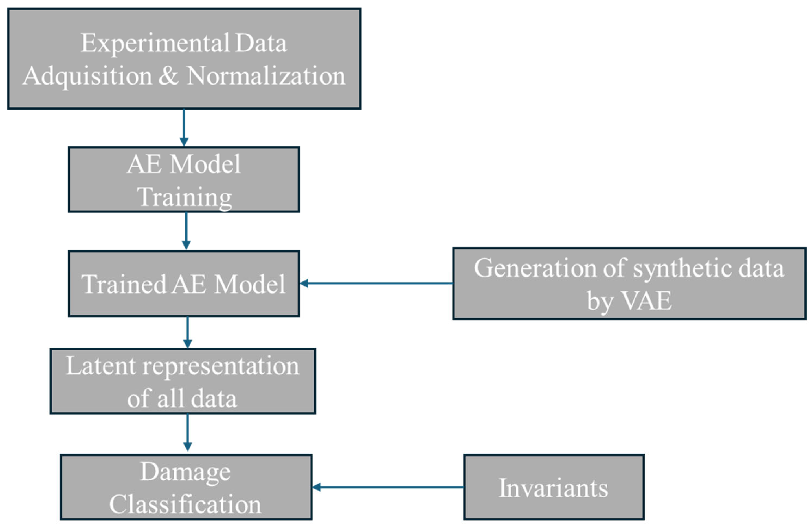
2. Methodology

An overview of the proposed scheme is shown in Figure 1. It is divided into five phases: (a) collection and normalization of an experimental dataset of EMI signals for different PZT transducers bonded on the target structure under different damage conditions; (b) generation and training of a deep autoencoder model from the experimentally collected training data for damage-sensitive features; (c) configuration and training of a variational autoencoder for the generation of synthetic data for the different damage stages and sensors considered in the experimental tests; (d) construction of the latent representations of all data, experimental and synthetic, emerging from the trained autoencoder model; and (e) damage identification from the distribution of all data in the latent space by means of the application of indicators based on manifold invariance.

More details about each one of these tasks are given in subsequent sections.

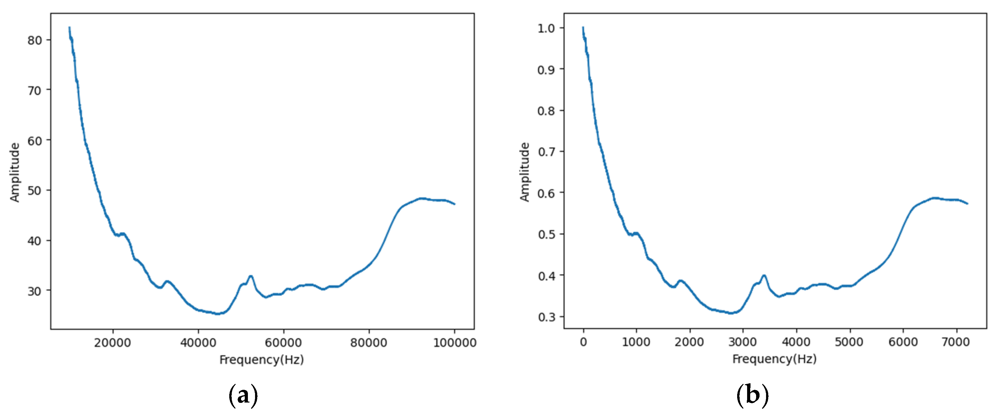
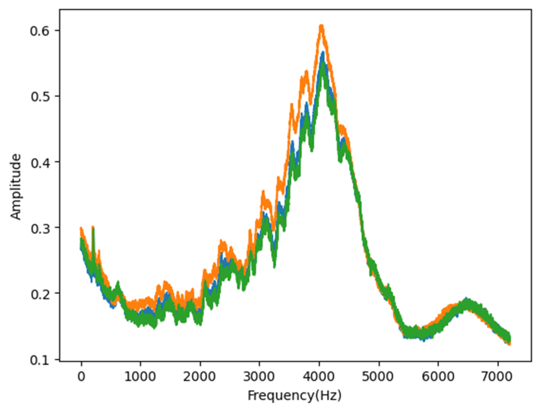
2.1. Collection of Dataset and Data Normalization: EMI Method

The proposed scheme assumes that EMI responses of an FRP-strengthened reinforced concrete beam under different damage conditions are captured using PZT sensors and an impedance analyzer (in this work, the Agilent HP 4192A analyzer, Santa Clara, CA, USA). For this, different sensors are bonded at different beam locations to measure a range of electromechanical impedance responses in the frequency domain.

Liang et al. [36] first introduced the EMI method to a one-dimensional model. This is shown in Equation (1), which gives the relation between the electrical admittance (inverse of the impedance, Z) of the PZT, Y(ω), and the mechanical impedance of the structure. Mechanical variations in the structure due to damage might be identified by means of admittance measurements.

$$\mathrm{Y}\left(\omega \right)=\mathrm{j}\omega {\displaystyle \frac{\mathrm{w}\mathrm{l}}{\mathrm{h}}}\left({\overline{\epsilon }}_{33}^{\mathrm{T}}-{\displaystyle \frac{{\mathrm{Z}}_{\mathrm{s}}\left(\omega \right)}{{\mathrm{Z}}_{\mathrm{s}}\left(\omega \right)+{\mathrm{Z}}_{\mathrm{a}}\left(\omega \right)}}{\mathrm{d}}_{3\mathrm{x}}^2{\widehat{\mathrm{Y}}}_{\mathrm{x}\mathrm{x}}^{\mathrm{E}}\right)$$

(1)

where Z_s and Z_a are the mechanical impedance of the host structure and the PZT sensor, respectively; w, l, and h are the width, length, and height of the PZT sensor, respectively; ${\overline{\epsilon }}_{33}^{\mathrm{T}}={\epsilon }_{33}^{\mathrm{T}}\left(1-\delta \mathrm{j}\right)$ and ${\widehat{\mathrm{Y}}}_{\mathrm{x}\mathrm{x}}^{\mathrm{E}}$ are the electrical permittivity at the zero electric field and the complex Young’s modulus of the PZT at zero stress, respectively; δ denotes the dielectric loss factor of the PZT; and d31 is a coupling piezoelectric coefficient [37].

Additionally, with the purpose of accelerating and improving the training of the neural networks used in the procedure, impedance data are preprocessed by means of a min–max normalization, as follows:

$$Z_{normalized}={\displaystyle \frac{Z-\mathrm{m}\mathrm{i}\mathrm{n}\left(Z\right)}{\max \left(Z\right)-\mathrm{m}\mathrm{i}\mathrm{n}\left(Z\right)}}$$

(2)

where $Z_{normalized}$ represents the computed normalized impedance spectrum.

Figure 2 shows an example of an impedance spectrum before and after normalization.

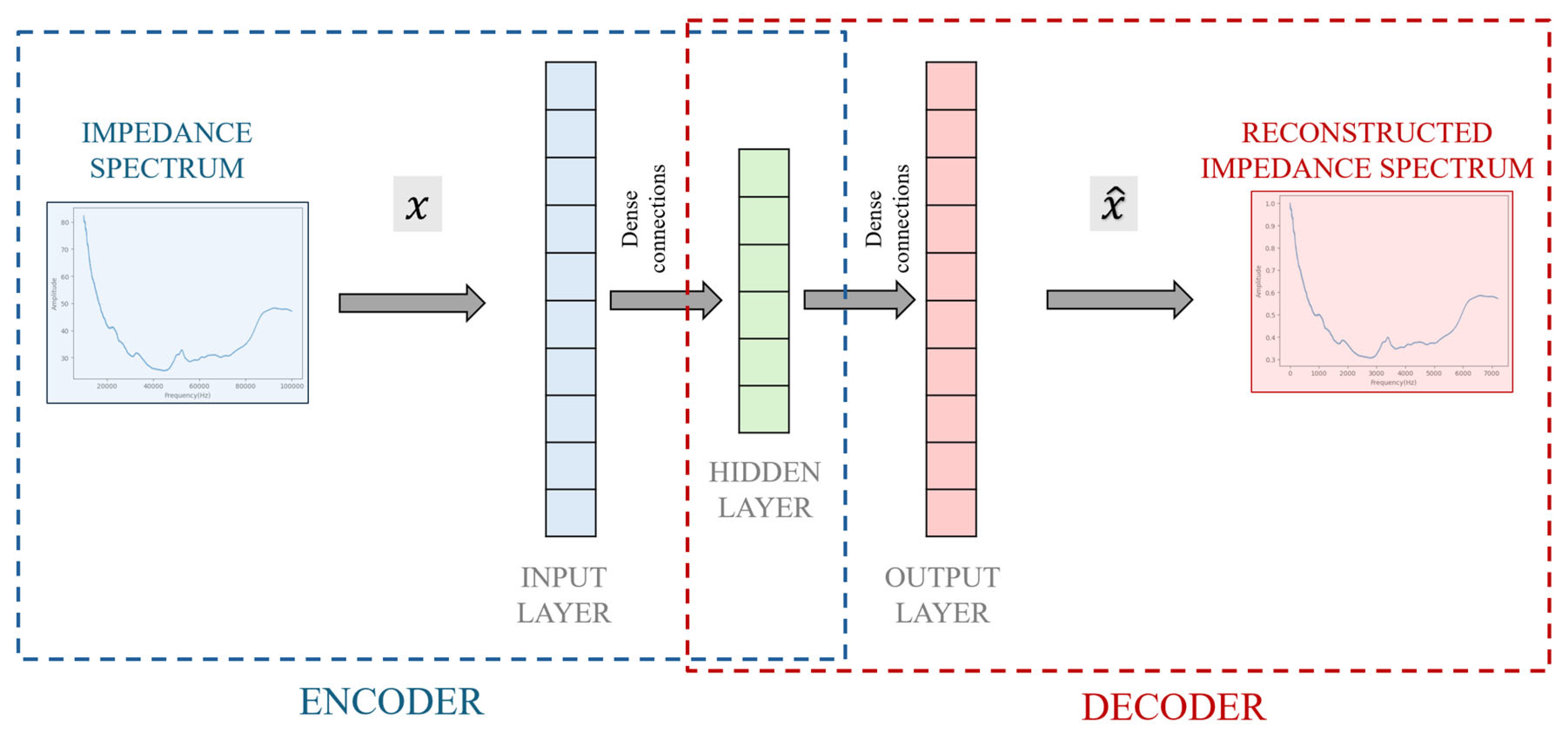
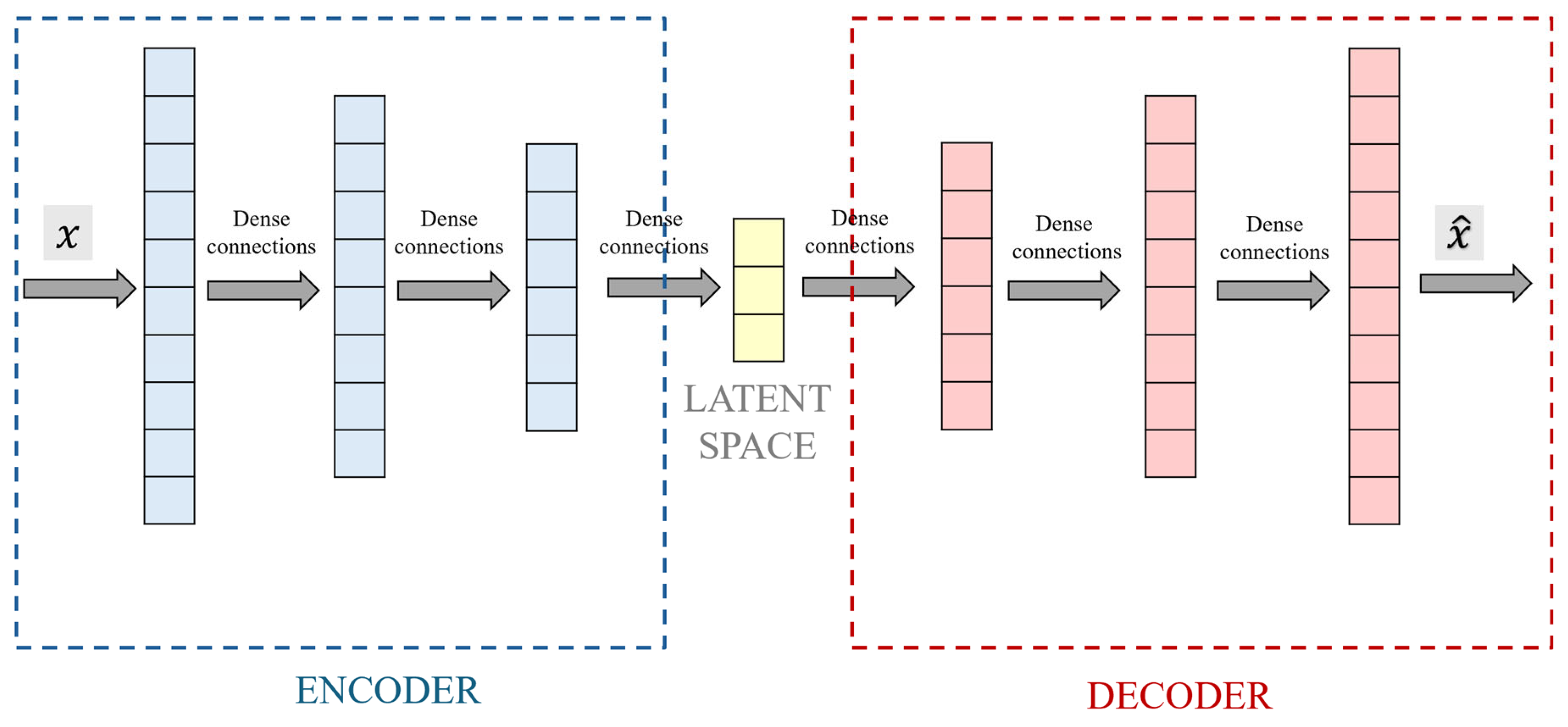
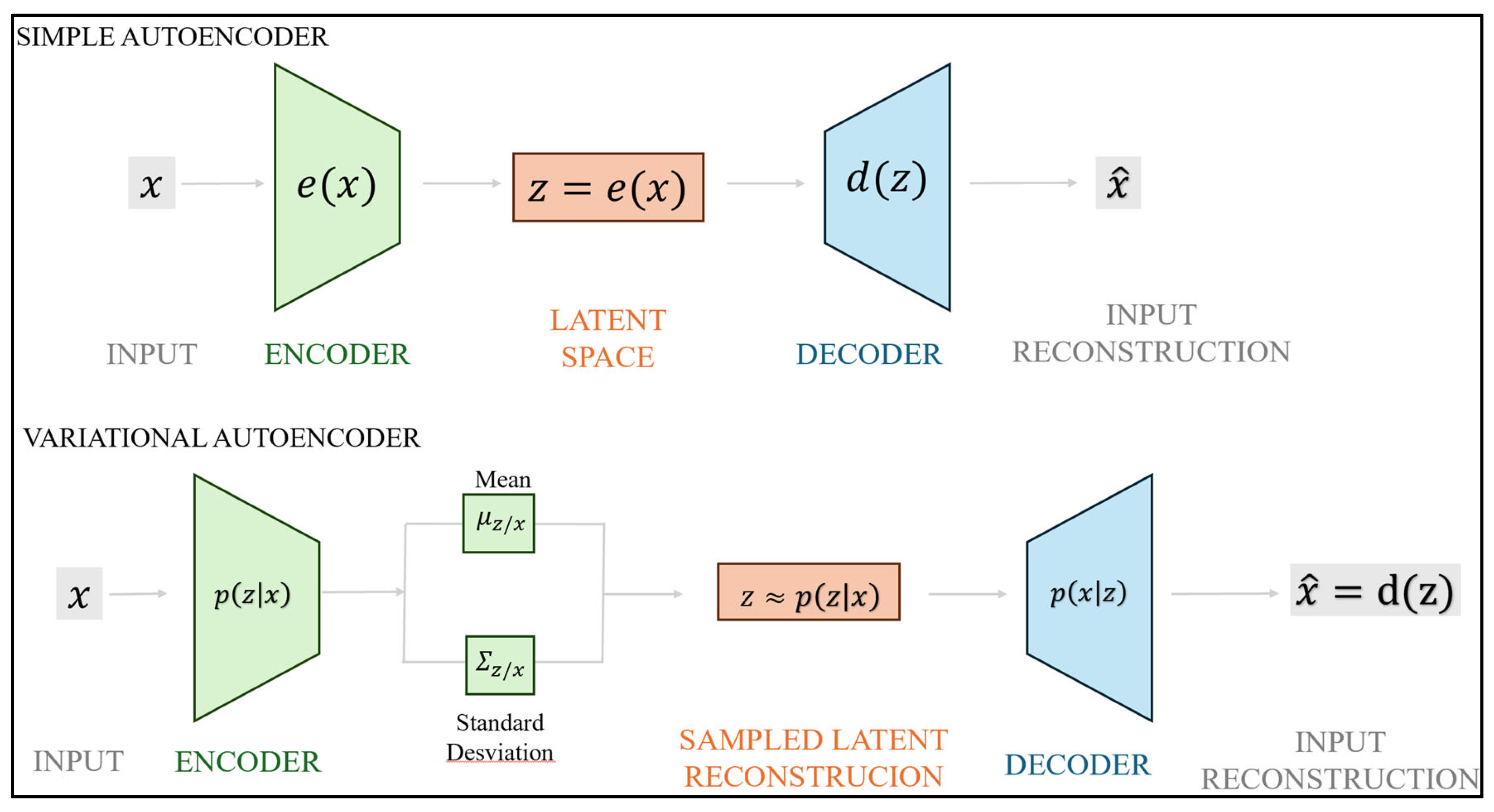
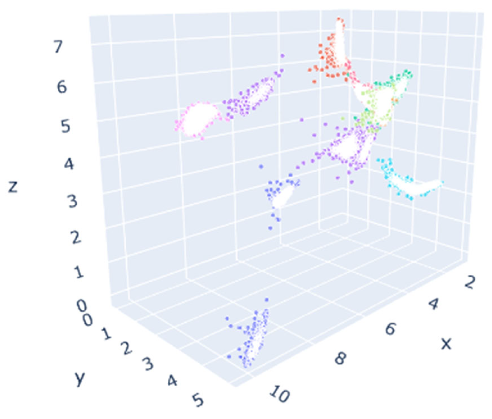
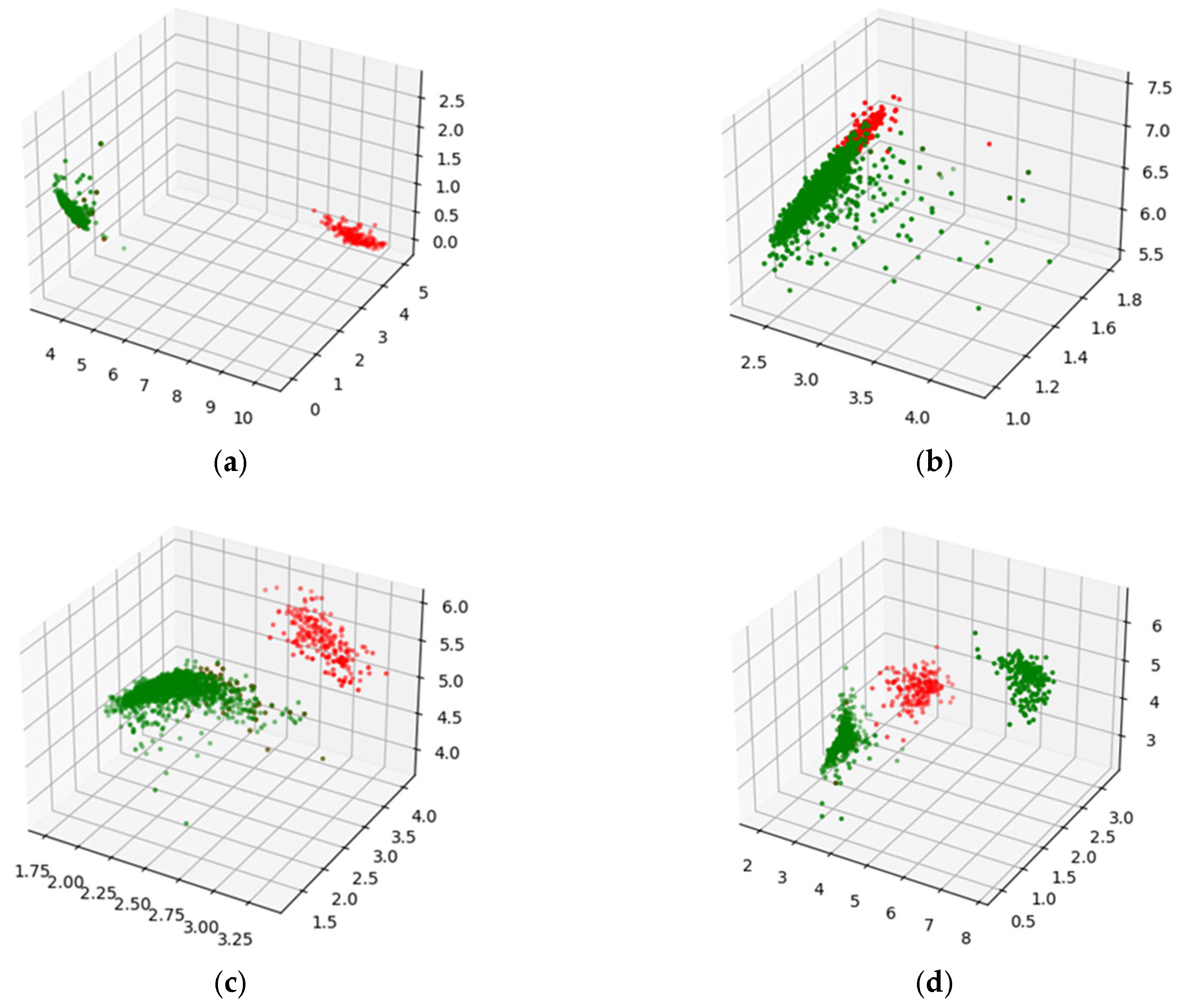
2.2. Deep Autoencoders: Latent Space Classification

Autoencoders are unsupervised neural networks that can handle large amounts of data and can also be applied to reduce the dimension of input data, extracting their most important features. The simplest configuration of an autoencoder is based on an encoding layer and a decoding layer, as shown in Figure 3. By means of the encoder, the input data, x, are mapped into an arbitrary lower dimensional space, h. The decoder reconstructs the original data as an output $\widehat{\mathit{x}}$ from h [18]. Therefore, the input and its corresponding output should be as identical as possible to each other. In this sense, the optimal autoencoder corresponds to the encoding–decoding scheme, keeping the maximum amount of information when encoding and providing a minimum reconstruction error of the input data when decoding.

The transfer function of each module can be expressed as follows:

$$\mathit{Encoder} \mathit{h}=f\left(\mathit{x}\right)=\phi \left(\mathit{W}\mathit{x}+\mathit{b}\right)$$

(3a)

$$\mathit{Decoder} \widehat{\mathit{x}}=g\left(\mathit{h}\right)=\phi \prime \left(\mathit{W}\prime \mathit{h}+\mathit{b}\prime \right)$$

(3b)

where (W, b) and (W′, b′) are the weight matrices and bias vectors for encoder and decoder modules, respectively, while $\phi$ and ${\phi }^{\prime }$ are the activation functions of the encoder and decoder, respectively. Nonlinear activation functions, such as sigmoids or hyperbolic tangents, are usually applied. Training of the autoencoder consists of updating the learning parameters, W, W′, b, and b′, by minimizing an error or loss function defined between input x and its reconstruction at the decoder’s output, $\widehat{\mathit{x}}$, which quantifies the error between both. The root mean squared error (RMSE), computed from the number of observations used for the training of the model, n, is frequently used for this purpose.

$$RMSE=\sqrt{\sum _{i=1}^n{\displaystyle \frac{{\left({\widehat{\mathit{x}}}_i-{\mathit{x}}_i\right)}^2}{n}}}$$

(4)

In the case of working with deep autoencoders, the encoding module is configured by a succession of layers with an increasingly smaller number of neurons, as if it were a bottleneck (Figure 4). This configuration allows for the progressive reduction in the dimension of the input neuron space, progressively extracting its most important features. The last layer of the encoder is the latent space, and it provides the most compressed representation of the input data. The effect of the decoder is to reconstruct the input neurons, in the most reliable way possible, through a series of layers in which the number of neurons increases, until it matches the dimension of the input space.

Assuming N hidden layers for both the encoder and decoder, the encoding representation can be expressed as a generalization of Equation (3a) as follows:

$$\begin{array}{c}{\mathit{h}}^{\left(1\right)}={\phi }^{\left(1\right)}\left({\mathit{W}}^{\left(1\right)}\mathit{x}+{\mathit{b}}^{\left(1\right)}\right)\\ ⋮\\ {\mathit{h}}^{\left(N\right)}={\phi }^{\left(N\right)}\left({\mathit{W}}^{\left(N\right)}{\mathit{h}}^{\left(N-1\right)}+{\mathit{b}}^{\left(N\right)}\right)\end{array}$$

(5)

where ${\mathit{h}}^{\left(i\right)}\left(1\le i\le N\right)$ is the encoded hidden representation, (${\mathit{W}}^{\left(i\right)},{\mathit{b}}^{\left(i\right)})\left(1\le i\le N\right)$ represent the network’s weights and biases, and ${\phi }^{\left(i\right)}\left(1\le i\le N\right)$ are the activation functions for the encoder.

On the other hand, the decoding will reconstruct the input vector through the following transformation:

$$\begin{array}{c}{\mathit{h}}^{\left(N+1\right)}={\phi }^{\left(N+1\right)}\left({\mathit{W}}^{\left(N+1\right)}{\mathit{h}}^{\left(N\right)}+{\mathit{b}}^{\left(N+1\right)}\right)\\ ⋮\\ \widehat{\mathit{x}}={\phi }^{\left(2N\right)}\left({\mathit{W}}^{\left(2N\right)}{\mathit{h}}^{\left(2N-1\right)}+{\mathit{b}}^{\left(2N\right)}\right)\end{array}$$

(6)

where ${\mathit{h}}^{\left(i\right)}\left(N+1\le i\le 2N\right)$ is the decoded hidden representation, (${\mathit{W}}^{\left(i\right)},{\mathit{b}}^{\left(i\right)})\left(N+1\le i\le 2N\right)$ represent the network’s weights and biases, and ${\phi }^{\left(i\right)}\left(N+1\le i\le 2N\right)$ are the activation functions for the decoder.

The identification of anomalies, such as structural damage, with traditional autoencoders is based on the measurement of a reconstruction error between the input data, x, and the reconstructed output, $\widehat{\mathit{x}}$, whenever the network has only been trained with non-anomalous data. However, this approach does not exploit the hierarchical nature of these models, which provides compact representations of the data and would allow for the detection of damage to smaller-dimension hidden spaces of the autoencoder. For the limiting case, the latent space captures the lowest-dimensional compressed space or, in other words, the main features of the input data. An exploration of the sampling points in the latent space gives insights into the distribution of the data. Latent space representations can be employed for damage detection by identifying those data points whose deviation regarding the learned patterns with healthy data is significant.

In this work, unlike usual procedures, the proposed structural health indicators were directly built in the latent space of a deep autoencoder model instead of in the output layer. For this, a new unsupervised clustering approach based on the latent space was developed for damage monitoring purposes. Clustering is difficult to carry out in high dimensions. However, by means of the latent space, the high-dimensional impedance spectra, captured with the different PZT sensors installed on the monitored structure, can be represented in a lower-dimensional space. Each impedance observation, x, corresponding to any stage of the structure, is mapped to its latent compressed representation, z. In this way, latent representations of experimental observations of different classes are clearly delimited in a low-dimensional space. Subsequently, latent representations of new data emerging of the trained autoencoder configure a net around the learned examples from each class of the dataset. New data points with their variations are encompassed to these nets, on which a clustering or classification algorithm can be applied. By using a distance-based clustering algorithm, if a new data point is fed into the trained network, its distance to the existing cluster centers is measured to determine if it is added to a cluster or forms a new cluster representative of a new damage stage or an anomaly regarding the existing clusters. In this work, a nonspecific clustering algorithm was applied quantitatively. As will be seen in Section 3.5, only a visual analysis was performed.

The preservation of the equivariance of the input data [38] through the encoding procedure is necessary for the identification process, since this allows for compressions while maintaining the similarity and dissimilarity among the classes. In this way, latent space representations of a deep autoencoder model, designed to extract the main damage-sensitive features from the impedance spectra captured with the different PZT sensors installed on the structure, are used as a preprocessing step for a subsequent clustering or classification step of the damage state of the structure.

2.3. Synthetic Data Generation with Variational Autoencoders

Intuitively, in the autoencoder models, the deep and nonlinear complex architectures of the encoder and the decoder are able to provide greater dimensionality reductions while maintaining a low amount of reconstruction loss. However, in the absence of any regularization, autoencoders can lead to severe overfitting with a latent space lacking any structure and organization, which makes it impossible to generate new meaningful data.

Unlike traditional autoencoders, VAEs are a kind of deep generative model whose implementation introduces a probability-based approach of deep autoencoders. In this way, a continuous latent space distribution is modeled by generating synthetic diverse and novel data samples with realistic variations. This approach allows for the capture of patterns not available in the original dataset.

The architecture of VAEs is similar to traditional autoencoders. However, unlike traditional autoencoders, VAEs are implemented within a probabilistic framework, which allows for the generation of new data points. In other words, encoders of traditional autoencoders reproduce fixed points in the latent space, while the encoder of VAEs does not produce single points but a distribution, usually Gaussian, over the latent space, characterized by a mean and a variance. By sampling from the distribution of the latent space and subsequent reconstruction with the decoder, new data points are generated, synthetically augmenting the original dataset.

To achieve this purpose, VAEs are trained by minimizing a loss function which combines two terms. On the one hand, one term measures the accuracy of the reconstruction provided by the decoder from an original input. This term is similar to that used to train traditional autoencoders. The second term includes a KL (Kullback Leibler) divergence regularization term whose purpose is to ensure that the learned latent probability distribution resembles a Gaussian distribution. This regularization term avoids overfitting and gives the latent space the ability to generate new data, which is the main reason to consider VAEs as deep generative models.

Figure 5 shows the difference between a deterministic traditional autoencoder and a probabilistic variational autoencoder. VAEs introduce probabilistic encoders and decoders. A probabilistic encoder, defined by p(z/x), describes the distribution of the encoded variable given the decoded one, while a probabilistic decoder, defined by p(x/z), describes the distribution of the decoded variable given the encoded one. In VAEs, the input is constrained to be encoded as a normal distribution over the latent space. Then, the decoding process is performed on sampled points from that distribution. Finally, the reconstruction error on these sampled points is backpropagated through the network for training. In this case, training is required not only to guarantee the performance of the encoding–decoding scheme, as usual, but also to organize the latent space by means of standard normal distributions as a result of the encoding procedure (regularization process), for which the mean and the covariance matrix of the normal distributions must be returned.

In this way, VAEs provide a more effective and diverse use of the latent space, which makes it possible to work with a wider range of variations in the input data. By means of this capacity, all the dimensions of the latent space are explored instead of relying on only a few. This feature can become very powerful in applications such as damage monitoring and synthetic data generation. As VAEs are generative models, not only do they learn to compress and reconstruct the data, but they are also able to generate new data by sampling from the latent space and following the learned distribution of the training set. VAEs are very powerful for synthetic data generation tasks because of their ability to learn a probabilistic latent space representation from complex data architectures, which allows them to capture the underlying structure of the training dataset. This makes them especially useful for those problems whose availability of data for network training is scarce and imbalanced. By using VAEs, the quality of a dataset can be enhanced by producing more representative and diverse simples based on trends learned from real data. The development of a robust system able to recognize and react to a variety of damage patterns, potentially not observed in the training dataset, is vital for our work, and, therefore, VAEs were used here as a tool to generate synthetic data.

2.4. Damage Identification

Usually, when working with autoencoders, the damage or novelty index is identified by means of the reconstruction or loss error computed from an autoencoder model previously trained with healthy data. This error measures the residual between the input data and the reconstructed data. When the trained model is fed with test data, a residual higher than a threshold, defined from the training data, can be considered as the symptom of an anomaly or damage, and the more the anomalies, the greater the residual.

However, although this is a standard procedure, as noted in Section 2.2, this way of proceeding does not take full advantage of the main strengths of autoencoders, i.e., hierarchical dimensionality reductions and high feature extraction capabilities. One of the main features of autoencoder models is that by means of successive layers of encoding–decoding hierarchical, low-dimension representations of both input and reconstructed data are learned; this might be exploited for damage identification purposes by defining damage indicators directly from the hidden spaces instead of from the output layer.

With these premises, in this work and unlike most traditional approaches, the latent space was used for damage monitoring purposes by means of a procedure applied on hybrid data, constituted by the original experimental and synthetic data, and based on three damage indicators: density, volume of the convex hull, and ellipse overlap. These indicators provide comprehensive insights into the structural integrity and potential damage within the monitored beam. A qualitative description of each one of these indicators is presented next.

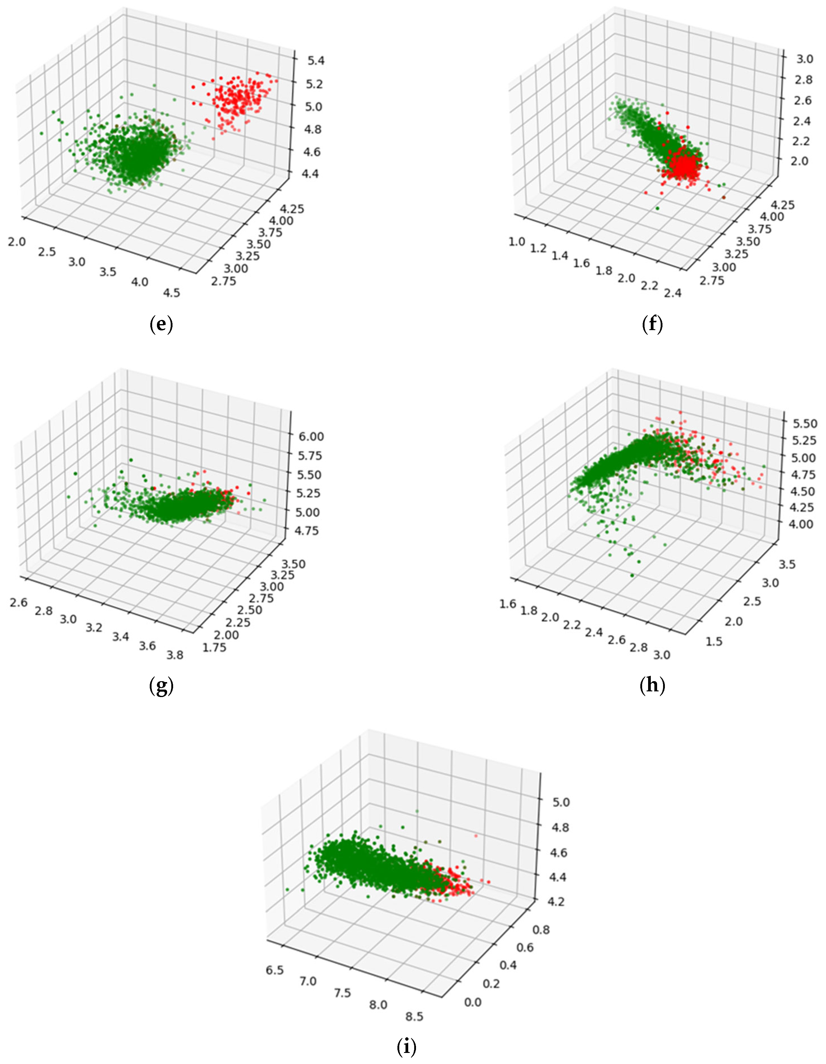
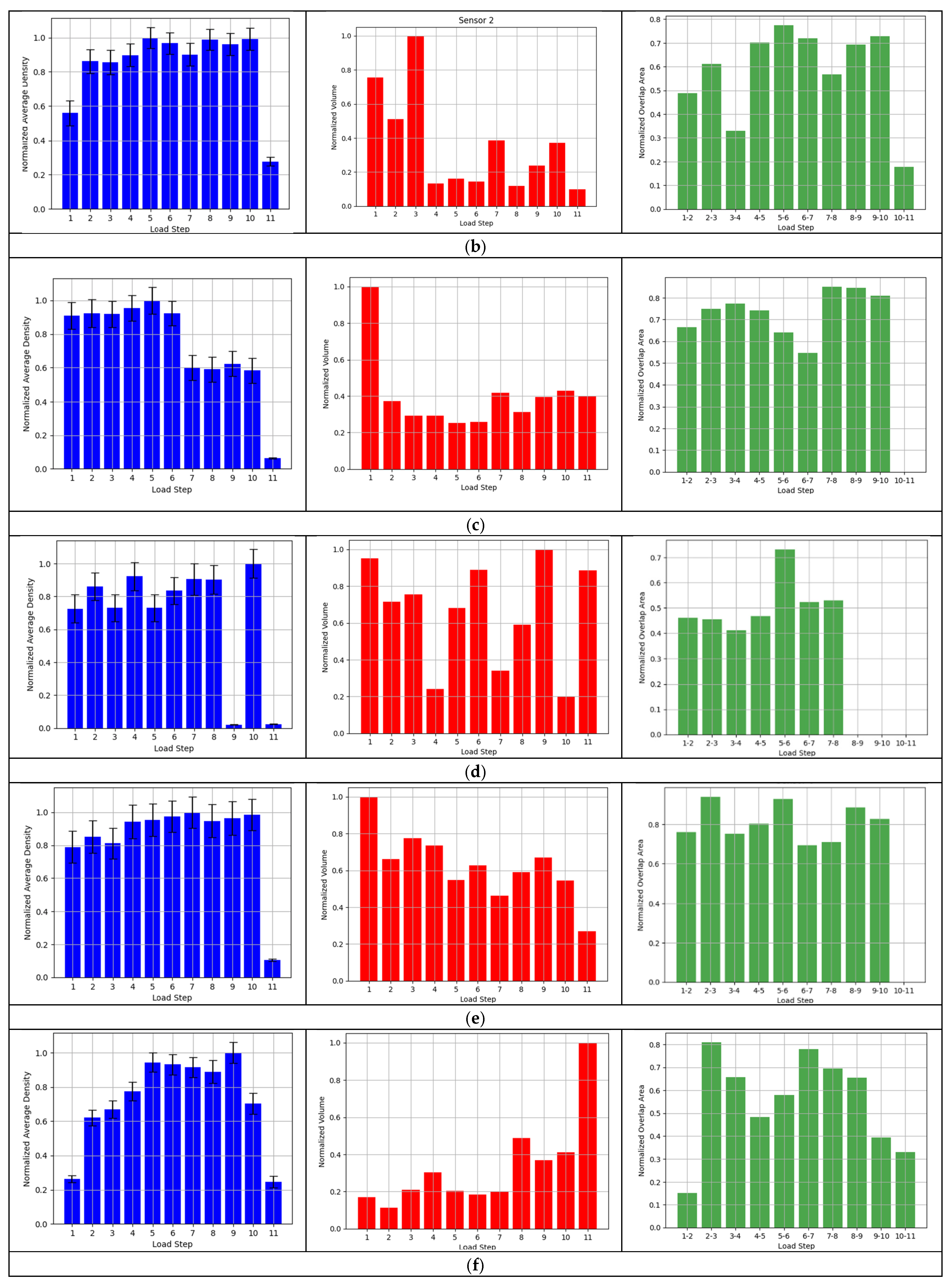
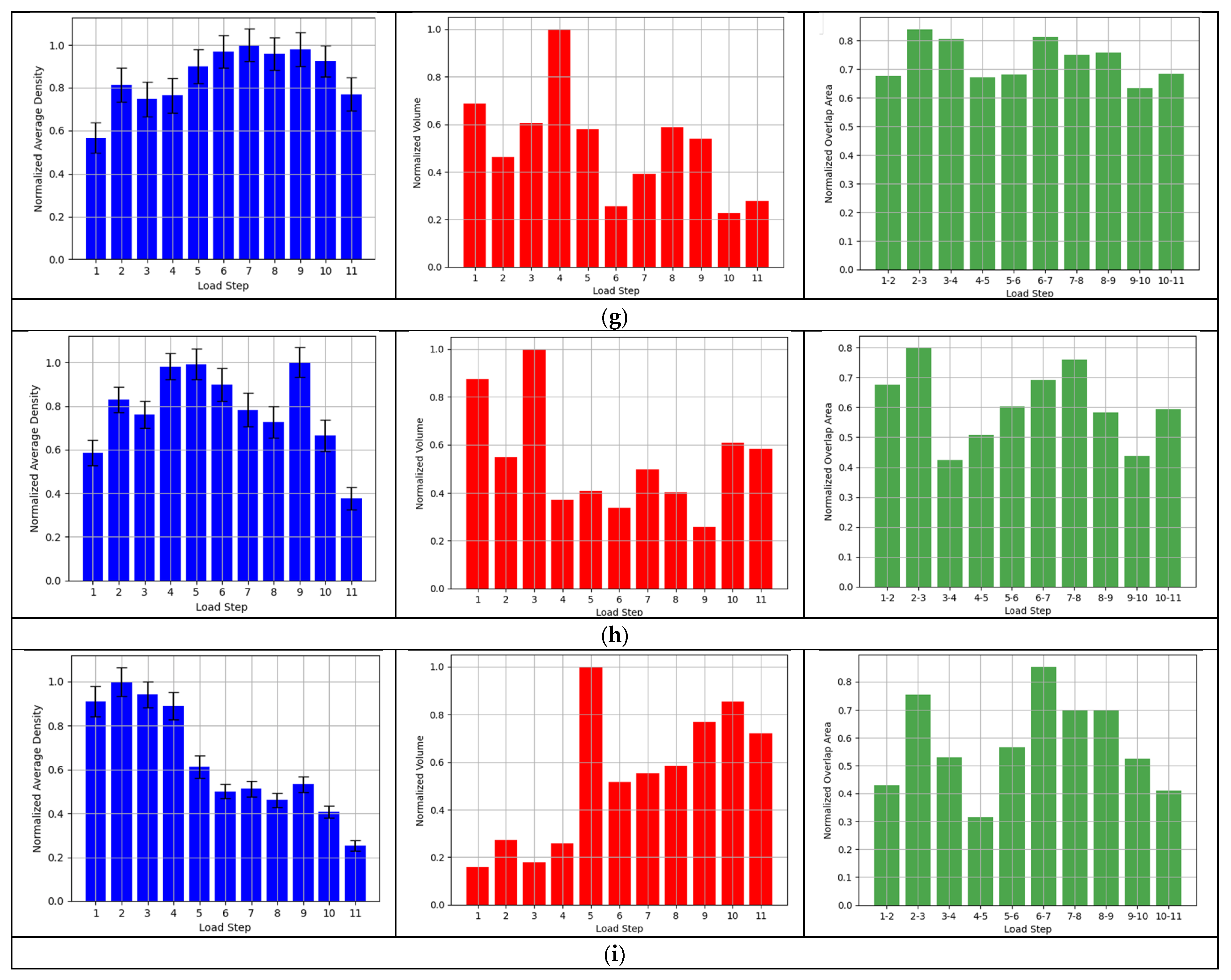
2.4.1. Density

Density measures the concentration of data points within a specific region of the latent space. This indicator is crucial for detecting structural anomalies, as it consistently reflects the structural cohesion of the beam across various tests and sensor locations. High density implies that data points are closely packed, suggesting a cohesive structure, whereas low density indicates dispersed data points, implying structural variability or potential damage.

The estimation of density is made by means of the kernel density estimation (KDE). KDE allows for the estimation of univariate and multivariate underlying probability density functions of a dataset whose distribution is unknown [39,40]. With this approach, the probability density function of a random variable from an unknown distribution for any real value of x is computed as follows:

$${\widehat{f}}_x^h={\displaystyle \frac{1}{m}}\sum _{i=1}^m{K}_h\left(x-x_i\right)={\displaystyle \frac{1}{mh}}\sum _{i=1}^{m}K\left({\displaystyle \frac{x-x_i}{h}}\right)$$

(7)

where K is the kernel smoothing function; m is the number of observations; h is the bandwidth; and x₁, x₂, …, x_m are the observations whose distribution is unknown. Different smoothing functions can be used. In this work, a Gaussian kernel with a bandwidth of 0.5 was used.

By means of KDE, a two-dimensional (2D) map of the average density is created from the latent space projection. In this way, a detailed observation of how density varies under different loading conditions is obtained, highlighting areas where structural behavior can experience changes. By normalizing density values, each average density is divided by the maximum observed density, facilitating the comparison of relative density changes across different loading steps and thus more effectively identifying patterns and anomalies.

Density is a valuable indicator, because it provides insights into the internal consistency and uniformity of the beam’s structural response. High-density regions correspond to stable and predictable structural behavior, while regions of low density can indicate areas of concern where the structural integrity may be compromised.

Data density in the latent space can be considered as a useful invariant to detect structural anomalies. When the beam is healthy, the density of data points is consistently controlled within a specific region. When damage occurs, the density distribution changes significantly, spreading out across the latent space. This change in density is invariant to the initial and final states, making it a powerful indicator of structural integrity changes.

2.4.2. The Volume of the Convex Hull

The volume of the convex hull is a geometric indicator that measures the total three-dimensional space occupied by the data points in the latent space. This volume is enclosed by the smallest convex polyhedron that can contain all the points. In SHM, this indicator captures the spatial dispersion of sensor data under varying load conditions, providing a quantitative metric of changes in structural integrity.

This indicator is particularly valuable, as it accounts for both the dispersion and the spatial arrangement and alignment of the data points. Such geometric configurations can reveal subtle changes or anomalies in the inspected structure, like the initiation of cracks or the propagation of existing damage, which might not be detectable through density measurements alone. Normalizing the convex hull volume by the maximum volume across different load steps contributes to the maintenance of a consistent scale for comparison, thus enhancing interpretability and visualizations.

The convex hull volume helps in understanding how structural responses spread out in the latent space. An increase in volume might indicate the development of structural anomalies, such as cracks or damage, that alter the beam’s overall geometry. This indicator can be used as a complement of density by offering a broader perspective on how structural changes affect the latent space. It provides a new perspective to the analysis by including the total spatial extent as well as the shape of the data. Changes in volume might be associated with damage growth that does not alter density but might affect the geometric distribution of the points in the latent space.

The convex hull volume provides a measure of the spread and dispersion of data points in the latent space, which is invariant with respect to coordinate rotations, translations, and scaling. Because of this, this representation is suitable for classification. When the beam is intact, the volume is constrained. However, as damage develops, the volume increases and spreads unpredictably. This shift is invariant to the initial and final states, effectively reflecting the transition from a controlled to a damaged state.

2.4.3. Ellipse Overlap

Ellipse overlap is an indicator which measures the similarity in the dispersion and orientation of data between consecutive load steps by comparing the overlap of ellipses that represent the data distributions. A high degree of overlap suggests minimal changes in structural characteristics, indicating stability, while a low degree of overlap means significant variations, which might potentially indicate damage.

To calculate the ellipse overlap, the data distributions are projected into a two-dimensional space, and ellipses are fitted to these projections. The overlap area between ellipses from consecutive load steps is then computed and normalized by dividing each overlap area by the maximum observed area. This normalization ensures a consistent scale for comparing the similarity in data distribution across different load conditions.

An overlap matrix provides a detailed representation about how the ellipses overlap each other. Elements of this matrix measure the level of overlapping. By working with normalized values, these elements should be between 0 and 1. Values close to one indicate a high degree of overlapping, while values close to zero mean a low degree of overlapping. Logically, the terms of the principal diagonal of the matrix should be equal to one, since they measure the overlapping of an ellipse with itself.

Ellipse overlap provides an additional perspective by focusing on the evolution of structural characteristics under different loading conditions. Unlike density and the convex hull volume, which address concentrations and spatial extents, ellipse overlap directly assesses the similarity in data distribution, thus capturing dynamic structural changes.

The invariant in this case is the degree of overlap between ellipses representing consecutive load steps. In a healthy beam, the degree of overlap is high, indicating stability and consistency in structural behavior. As damage occurs, the degree of overlap decreases significantly, reflecting changes in the structural response. This reduction in the degree of overlap is invariant to the specific initial and final stages, making it a reliable indicator of structural changes.

2.4.4. An Ensemble Application of the Indicators

Each one of the three indicators has pros and cons. However, handicaps of some might be compensated for by the strengths of others. Therefore, an ensemble application of these indicators might offer a robust framework for health monitoring of structural components. The three indicators would complement each other by covering different aspects of data behavior in the latent space:

• Density provides insights into the concentration and cohesion of data points.
• The volume of the convex hull captures the overall spatial dispersion and geometric configuration.
• Ellipse overlap assesses the dynamic similarity in data distribution between consecutive load steps.

Together, they can provide a comprehensive view of structural integrity, which can help to detect, localize, and understand potential damage in the monitored structures. By integrating these indicators, a more nuanced and detailed picture of structural health can be achieved, enhancing the effectiveness of SHM systems.

3. Experimental Validation

The proposed methodology was validated on an experimental case involving the damage identification of an externally bonded FRP-strengthened RC beam. This type of strengthening is a good touchstone because of its typical failure modes and its local origin.

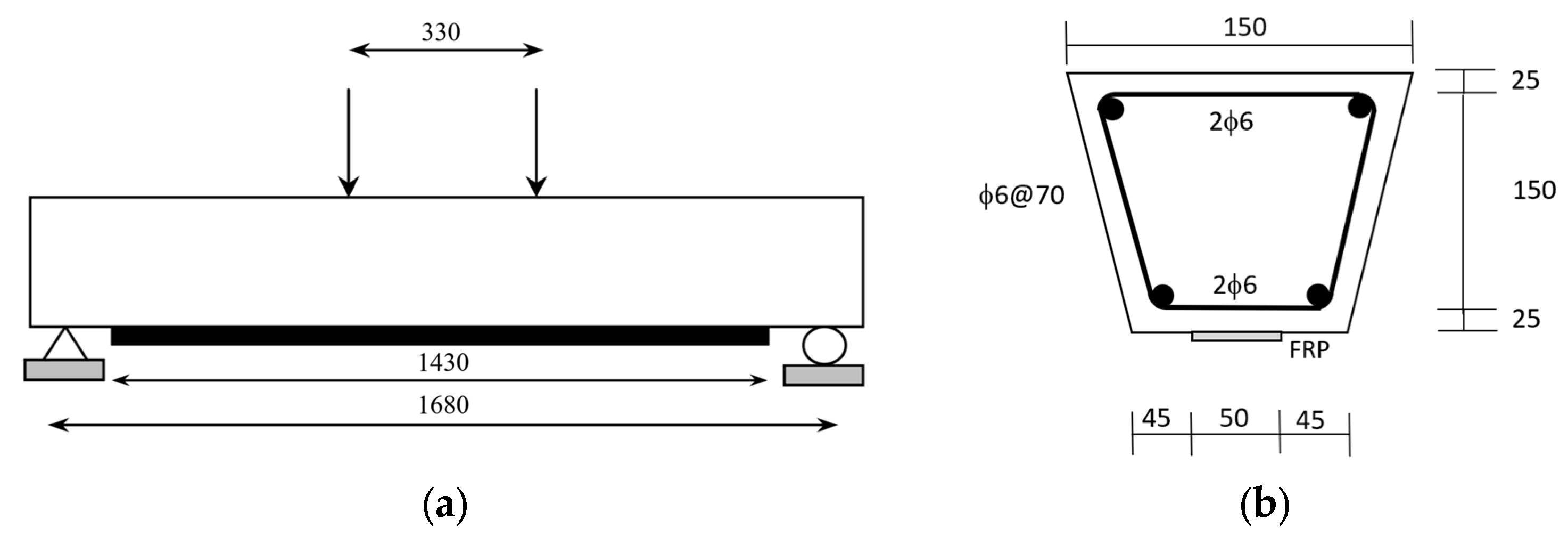
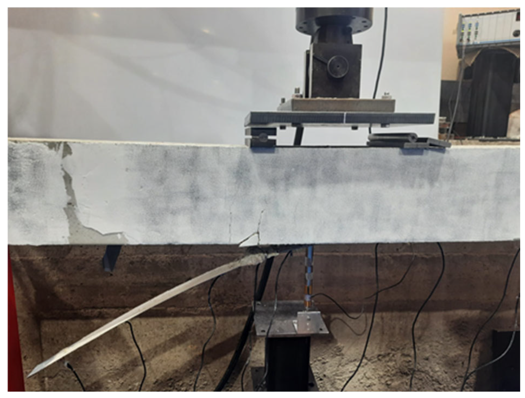
3.1. Experimental Set-Up

One reinforced concrete beam externally bonded with an FRP strip was tested until failure to study the characteristics of impedance spectra in the failure process [37]. The configuration of the beam together with the trapezoidal cross-section are shown in Figure 6. The geometric characteristics of the beam as well as the diameter of the steel reinforcements are shown in the figure.

The material properties were as follows: (a) Concrete with compressive strength = 35 megapascal (MPa) and tensile strength = 3 MPa was used. (b) Steel with yield strength = 500 MPa and elastic modulus = 210 gigapascal (GPa) was used. (c) One FRP strip (Sika CarboDur S512, Sika, Lyndhurst, NJ, USA) of 1430 mm in length × 50 mm in width × 1.2 mm in thickness was used for strengthening. The tensile strength of the FRP strip was 3100 MPa, and the Young’s modulus was 170 GPa. Two-part epoxy was used to attach the FRP plate to concrete.

The beam specimen was tested under four-point bending (Figure 6). Electromechanical impedances were captured during the tests by means of nine PZT patches (Figure 7) bonded to the FRP strip. P-876.A11 and P-876-SP1 PZT types were used, except for close to the ends of the FRP strip, where P-876.A15 (61 mm × 35 mm × 0.8 mm) sensors were glued [41].

The tested beam was loaded following a sequence of 16 loading–unloading steps until failure with a maximum value of the loading force for each step, as shown in

Table 1. Sequence of static loading tests for the specimen.

Test Number	Load Level	Test Code
1	0 kN	1 (Baseline)
2	6 kN	2
3	14 kN	3
4	16 kN
5	25.6 kN
6	26.3 kN	4
7	31.3 kN	5
8	32 kN	6
9	38 kN	7
10	44 kN	8
11	47.9 kN
12	53.4 kN	9
13	63.8 kN
14	70 kN
15	85.5 kN
16	92 kN	10
17	94 kN	11

.

In each loading step, once the established load maximum was reached, the beam was completely unloaded, and the impedances were measured in all the sensors. Failure occurred due to the sudden detachment of the FRP strip as a consequence of the strong concentration of stresses that originated in the vicinity of a crack at the bottom of the beam, close to the left loading point. FRP debonding propagated towards the left end of the strip (Figure 8). Prior to failure, multiple cracks formed, first in the constant moment zone and, subsequently, in other areas of the beam. All of this extended cracking contributed to the subsequent failure of the beam. The first identified vertical crack occurred during test 3.

For each loading step and with the purpose of stabilizing the progressive cracks, a protocol of three cycles of loading and unloading were applied for each load step. To simplify this study, from the 17 tests shown in Table 1, this study only focuses on tests 1, 2, 3, 6, 7, 8, 9, 10, 12, 16, and 17. A test code (1 to 11) was assigned in the third column of Table 1 for your reference in subsequent figures.

3.2. Dataset

First, to apply the proposed methodology, an experimental dataset was collected and processed. The datasets used in this research were taken from the nine PZT sensors and the eleven load steps referenced in the third column of Table 1. The test codes included in this last column will be used to make reference to the analyzed load steps. The EMI signatures were acquired by the nine sensors using an Agilent 4294A impedance analyzer with a 1-volt (V) voltage excitation within a range of 10–100 kiloHertz (kHz) and with a step interval of 12.5 Hertz (Hz). Therefore, an impedance spectrum of 7201 points was fed to the deep AE and VAE models for each sensor and load step.

Regarding data preprocessing, the dataset was normalized by means of min–max scaling with the range [0, 1] (Equation (2)).

3.3. VAE Configuration: Data Augmentation

Damage identification, based on the classification of points defined in the latent space of an autoencoder model, requires a considerable amount of EMI signals, which are usually limited if only experimental tests are used. Therefore, a data augmentation technique should be applied to generate massive synthetic data, which will reduce overfitting issues and improve network performance.

As noted in Section 2.3, VAEs are capable of managing complex data distributions and generating new data artificially. In our problem, from a sampling of the latent space, VAEs can generate synthetic data covering a wide range of variations in the input data by leveraging probabilistic latent space and exploring all its dimensions. Data augmentation allows for the tackling of limited and imbalanced real-world experimental datasets.

In this work, a VAE model was fed with datasets belonging to the different analyzed loading stages and PZT sensors, which means distinct impedance input distributions with varying levels of class imbalance were used. This will serve to test the robustness of the VAE model when synthesizing realistic class imbalance datasets.

The configuration of the VAE model was obtained with a batch size, learning rate, and number of epochs of 16, 0.0001, and 4600, respectively, with the purpose of optimizing its performance.

An encoder block and a decoder block were used to define its architecture (

Table 2. Variational autoencoder architecture.

Section	Layer Type	Input	Output	Activation
Encoder	Fully connected	7201	2000	PReLU
	Fully connected	2000	1000	PReLU
	Fully connected	1000	100	PReLU
	Fully connected	100	50	PReLU
Mean and log-variance of the latent space distribution	Fully connected	50	25 (Mean) 25 (Log-variance)
Decoder	Fully connected	25	100	PReLU
	Fully connected	100	1000	PReLU
	Fully connected	1000	2000	PReLU
	Fully connected	2000	7201	PReLU

). The encoder maps the input data corresponding to the impedance spectra dataset of dimension 7201 into a lower-dimensional latent space by means of successive dense layers which comprise 2000, 1000, 100, and 50 neurons, respectively. The parametric rectified linear unit (PReLU) activation function was used in all the layers. With this architecture, the essential information of the data is retained while reducing dimensionality progressively until reaching the latent space, whose dimension is 50. Although a smaller dimension provides a more compact representation of the input data, it might also cause the loss of important information. The dimension of the latent space must represent a compromise between the degree of compression of the data and the critical information they retain.

The latent space distribution is given by two parallel dense linear layers, which correspond to the mean and log-variance of the latent space distribution. The size of both layers agrees and is equal to the latent dimensionality which, in this case, was adjusted to 25. This hyperparameter was experimentally adjusted with the purpose of capturing the complexity of the input data, avoiding the loss of important information and maintaining computational efficiency. Both values, the mean and log-variance, are used for sampling the latent space and for the generation of a probabilistic latent space representation.

Beginning with the latent space, the decoder block is also defined with dense layers and using PReLU activation. Its architecture mirrors that of the encoder, with the aim of reconstructing the input data points by reversing the encoding steps.

In this case, the loss function used to control the training process has two components, the reconstruction loss, evaluated using MSE (mean squared error), and the Kullback–Leibler Divergence (KLD). While MSE measures the difference between the original and reconstructed data, KLD penalizes the model if the latent space distribution deviates from a standard normal distribution. A hyperparameter, β, weights the importance of MSE and KLD in the loss function. In this study, the same weight was given to both components of the loss function.

The minimization of the loss function as well as the updating of the weights of the model were performed with the Adam optimization algorithm, which can be considered as an extension of the stochastic gradient descent algorithm. Figure 9 shows the evolution of the loss function of the variational autoencoder during its training.

Once the VAE model was trained, synthetic data (artificial tests) were generated with it. Specifically, 200 synthetic impedance spectra were generated for each sensor and load step, making a total of 200 × 9 × 11 =19,800 new synthetic data points. Figure 10 shows some samples of the artificial spectra. The variability in the generation of synthetic data is an indication that the VAE model works correctly. After generating the new data with the VAE model, the synthesized data points were then combined with the original dataset, resulting in a balanced hybrid dataset which includes all classes. This dataset was available for the damage classification based on the predictive deep autoencoder model.

3.4. Deep Autoencoder Configuration

According to the dimensions of the impedance spectra captured with the PZT transducers and the synthetic data generated subsequently, this study arranged the input and output dimensions in 7209 × 1. Both the encoder and decoder of this proposed deep autoencoder architecture consist of three fully connected layers. The PReLU (Parametric Rectified Linear Activation) activation function was applied for all the layers. PReLU is a generalization of the traditional rectified unit, with a slope for negative values.

Table 3. Deep autoencoder architecture.

Section	Layer Type	Input	Output	Activation
Encoder	Fully connected	7201	4000	PReLU
	Fully connected	4000	100	PReLU
	Fully connected	100	3	PReLU
Decoder	Fully connected	3	100	PReLU
	Fully connected	100	4000	PReLU
	Fully connected	4000	7209	PReLU

provides a summary of the proposed deep autoencoder architecture. The model was implemented using PyTorch 2.4. An Adam optimization algorithm was used for training of the autoencoder. With this procedure, learning rates are adapted for each parameter or weight individually. The network was trained for 2200 epochs, using an initial learning rate of 0.0001. MSE was used to measure the loss functions. Its evolution is shown in Figure 11.

Only the original data were used for training, with the purpose of learning to represent these data in the latent space. This decision was adopted because of the higher reliability and precision provided by the original data. These data are essential to capture the main features of the measured spectra.

Once the network was trained, it was fed with all the synthetic data to extract their representation in the latent space. As the latent space is represented by the main three features of the input data, the hybrid dataset can be plotted in a 3D space, from which the analysis of invariants for further damage classification can be performed.

3.5. Analysis

Figure 12 shows the distribution of all data points (original and synthetic) in the three-dimensional latent space for all the sensors and all the analyzed loading stages (test codes 1 to 11 in Table 1). The clusterability of the latent representations for the different loading stages is evident, allowing for the distinction of intra-class similarities and inter-class dissimilarities. All the variants of the new data points, synthetically generated within the probabilistic framework introduced by the VAE, are perfectly encompassed in the classes defined by the original data. These features, not obvious in the original data, show patterns in the data and provide powerful mathematical signatures that are used in the proposed model to predict the health of the structure. This is one of the main ideas applied in this work.

In Figure 12, the data of all PZT transducers are included. If discrimination by the sensors is performed to represent the data points in the latent space, Figure 13 is obtained. With the purpose of remarking the transition from the lower to the higher damage states and to avoid excessive confusion in the figures, only the two higher damage states (tests 16 and 17), corresponding to the last two loading stages prior to the failure of the specimen, are represented in red, while for the other stages, green was used. PZT sensors work in a high frequency range and, therefore, are able to monitor local stiffness changes occurring in the vicinity of their location. Sensors located closer to the area of early damage will be able to capture this minor damage. However, sensors located further away will not be affected.

It is evident that the last loading stage (test number 17) formed a cluster far from the previous stages for those sensors located on the left side of the beam. This agreed with the failure mode of the beam, which occurred by debonding of the left side of the FRP strip (Figure 8). For the penultimate loading stage (test number 16), the growth of the damage was progressive. One important point to remark on regards sensor 4, for which three clusters were distinguished, affecting the intermediate loading stages. This phenomenon means that something noticeable occurred before reaching the last loading stages. Debonding originated close to this sensor as a consequence of a strong concentration of stresses that occurred near a major flexural crack.

The distance between the red and green clusters served to determine if, in the vicinity of each sensor, the damage grew more or less gradually for the last two stages. However, the graphs in Figure 13 may be misleading, because for some sensors, the data points corresponding to the penultimate loading step were mixed with those of previous loading steps and could not be distinguished. The existence of enough overlapping clusters and decreased cluster homogeneity is, without a doubt, one of the main limitations of clustering when applied to the latent space of autoencoders. The clusterability of latent representations could be the purpose of a deeper future study.

Figure 14 shows the evolution of the three indicators, average density (blue), volume of the convex hull (red), and ellipse overlap (green), presented in Section 2.4 to identify damage.

Related to the average density, a higher density should be obtained in the initial stages when the beam has experienced only minor damages. However, whenever damage progresses, the data points should spread out, decreasing the density. More dispersion might be the symptom of an anomalous performance of the beam, possibly due to damage. From the blue histograms in Figure 14, it is evident that, except for some cases (sensors 3 and 4), only significant variations in this parameter were obtained for the last loading stage, which is a symptom of the sudden debonding of the FRP plate. For sensor 3, from load step 7, an important deterioration occurred which was maintained until the last stage. For sensor 4, a sudden and very significant decrease in volume broke out in the ninth step. Debonding originated close to this sensor; therefore, this could have been a warning before the final failure. Although it holds less interest than clusterability itself, in the first column of Figure 14, the average density was also plotted for a 95% confidence interval.

The volume of the convex hull and the density of the points in the latent space provide complementary information about the state of the beam. Although both indicators might be inversely related in some cases, volume brings an additional dimension to the analysis by considering the total spatial extent and shape of the data, which might be crucial for more complex diagnoses. This parameter showed higher fluctuations than density throughout the loading steps, which might mean that it is very sensitive to the complex loading–unloading dynamic and that its efficiency is not as high as that of density.

Finally, ellipse overlap histograms (third column of Figure 14 in green) show how the similarity in data dispersion varied between consecutive loading steps. In general, a high degree of overlap between consecutive steps indicates that the beam structure has not changed significantly, while a low degree of overlap suggests notable variations, possibly due to damage. By analyzing these histograms, specific patterns of how the beam responds to different load levels can be identified. For the sensors located on the left side of the FRP strip, the overlap level between the last two loading stages was zero or near-zero, which is a symptom of the subsequent sudden debonding of the strip. It is remarkable that there was zero overlap among the last four loading stages for sensor 4, the origin of the subsequent debonding.

From this study, it can be concluded that a decrease in density, an increase in the hull volume, and a reduction in ellipse overlaps are complementary indicators suitable to determine the health of a structure, which agrees with what can be intuited with the visualization of the latent space.

4. Conclusions

In this work, a new methodology for structural damage identification was proposed. Some of the main novelties of this method are as follows: (a) Unlike usual procedures, damage was identified based on the latent space representation of a trained deep autoencoder instead of on the measurement of a reconstruction error between the input data and the reconstructed output of the autoencoder. (b) Clusterability of the latent representations emerging from the deep autoencoder around all classes of the original dataset was used for learning. New data points or synthetic data, generated with a variational autoencoder and providing new variants, are encompassed in the classes defined by the original data, contributing to the clustering of all datasets into classes. This unsupervised classification provides features to predict structural health. (c) Three damage indicators, average density, volume of the convex hull, and ellipse overlap, were defined from the latent space representation based on the preservation of the invariance in the input data through the encoding of the AE.

The model was illustrated and validated through a test case using actual experimental data obtained on an externally FRP-strengthened RC beam. The records of impedance of this specimen captured with nine different PZT sensors under different levels of loads and, therefore, of damage were used to fully verify the capability of the proposed method. The proposed model does not require costly and huge experimental results. The three indicators proved to be useful in identifying the progressive deterioration of the specimen and to predict the sudden debonding failure at its earliest stages.

With regards to future work, different approaches aimed at improving the model should be explored. One of these alternatives concerns the search and implementation of other indicators able to provide greater robustness to the model. This would enrich the set of metrics used for SHM, thus obtaining a more accurate model. More complex neural network architectures and advanced regularization techniques should also be explored to improve the accuracy and robustness of AE and VAE models.

Likewise, considering a more global perspective, the developed techniques should be validated with larger and more complex structures. In this way, the generalization and adaptability capacity of the proposed model could be assessed. Its application to large structures will provide a limited amount of data, in line with the limited number of sensors available. In this case, a preliminary study to guide optimal sensor configurations and locations for different classes of large-scale structures will be needed. Furthermore, temperature effects will influence EMI measurements and, therefore, could overwhelm the effect of damage, easily leading to false detections. For this, the proposed method should be reformulated to deal with thermal effects too.

Finally, another very important aspect to be explored in the future, which is gaining relevance in the last few years, concerns transfer learning. The ability of methods able to adapt the knowledge and classifier system built on this problem to solve other new scenarios for similar specimens should be addressed. This would be of significant interest for SHM of FRP-strengthened RC beams, since this would minimize costs and time in the monitoring systems.

References

- Zhao, R.; Yan, R.; Chen, Z.; Mao, K.; Wang, P.; Gao, R. Deep learning and its applications to machine health monitoring. Mech. Syst. Signal Process. 2019, 115, 213–237. [Google Scholar] [CrossRef]
- Ghiasi, A.; Moghaddam, M.K.; Ng, C.T.; Sheikh, A.H.; Shi, J.Q. Damage classification of in-service steel railway bridges using a novel vibration-based convolutional neural network. Eng. Struct. 2022, 264, 114474. [Google Scholar] [CrossRef]
- Zhou, X.Q.; Huang, B.G.; Wang, X.Y.; Xia, Y. Deep learning-based rapid damage assessment of RC columns under blast loading. Eng. Struct. 2022, 271, 114949. [Google Scholar] [CrossRef]
- Ai, D.; Cheng, J. A deep learning approach for electromechanical impedance based concrete structural damage quantification using two-dimensional convolutional neural network. Mech. Syst. Signal Process. 2023, 183, 109634. [Google Scholar] [CrossRef]
- Jiang, T.; Frøseth, G.T.; Rønnquist, A. A robust bridge rivet identification method using deep learning and computer visión. Eng. Struct. 2023, 283, 115809. [Google Scholar] [CrossRef]
- Ahmadian, V.; Beheshti Aval, S.B.; Noori, M.; Wang, T.; Altabey, W.A. Comparative study of a newly proposed machine learning classification to detect damage occurrence in structures. Eng. Appl. Artif. Intel. 2024, 127, 107226. [Google Scholar] [CrossRef]
- Lomazzi, L.; Giglio, M.; Cadini, F. Towards a deep learning-based unified approach for structural damage detection, localisation and quantification. Eng. Appl. Artif. Intel. 2023, 121, 106003. [Google Scholar] [CrossRef]
- Di Mucci, V.M.; Cardellicchio, A.; Ruggieri, S.; Nettis, A.; Renò, V.; Uva, G. Artificial intelligence in structural health management of existing bridges. Autom. Constr. 2025, 167, 105719. [Google Scholar] [CrossRef]
- Sony, S.; Dunphy, K.; Sadhu, A.; Capretz, M. A systematic review of convolutional neural network-based structural condition assessment techniques. Eng. Struct. 2021, 226, 111347. [Google Scholar] [CrossRef]
- Viotti, I.D.; Ribeiro, R.F., Jr.; Gomes, G.F. Damage identification in sandwich structures using Convolutional Neural Networks. Mech. Syst. Signal Process. 2024, 220, 111649. [Google Scholar] [CrossRef]
- Sattarifar, A.; Nestorović, T. Damage localization and characterization using one-dimensional convolutional neural network and a sparse network of transducers. Eng. Appl. Artif. Intel. 2022, 115, 105273. [Google Scholar]
- Wang, B.; Lei, Y.; Yan, T.; Li, N.; Guo, L. Recurrent convolutional neural network: A new framework for remaining useful life prediction of machinery. Neurocomputing 2020, 379, 117–129. [Google Scholar] [CrossRef]
- Barzegar, V.; Laflamme, S.; Hu, C.; Dodson, J. Ensemble of recurrent neural networks with long short-term memory cells for high-rate structural health monitoring. Mech. Syst. Signal Process. 2022, 164, 108201. [Google Scholar] [CrossRef]
- Pathirage, C.S.N.; Li, J.; Li, L.; Hao, H.; Liu, W.; Ni, P. Structural damage identification based on autoencoder neural networks and deep learning. Eng. Struct. 2018, 172, 13–28. [Google Scholar] [CrossRef]
- Ma, X.; Lin, Y.; Ma, H. Structural damage identification based on unsupervised feature-extraction via variational Auto-encoder. Measurement 2020, 160, 107811. [Google Scholar] [CrossRef]
- Zhang, Y.; Xie, X.; Li, H.; Zhou, B. An unsupervised tunnel damage identification method based on convolutional variational auto-encoder and wavelet packet analysis. Sensors 2022, 22, 2412. [Google Scholar] [CrossRef]
- Römgens, N.; Abbassi, A.; Jonscher, C.; Grießmann, T.; Rolfes, R. On using autoencoders with non-standardized time series data for damage localization. Eng. Struct. 2024, 303, 117570. [Google Scholar] [CrossRef]
- Yang, K.; Kim, S.; Harley, J.B. Unsupervised long-term damage detection in an uncontrolled environment through optimal autoencoder. Mech. Syst. Signal Process. 2023, 199, 110473. [Google Scholar] [CrossRef]
- Perera, R.; Montes, J.; Gomez, A.; Barris, C.; Baena, M. Unsupervised autoencoders with features in the electromechanical impedance domain for early damage assessment in FRP-strengthened concrete elements. Eng. Struct. 2024, 315, 118458. [Google Scholar] [CrossRef]
- González-Muñiz, A.; Díaz, I.; Cuadrado, A.; García-Pérez, D. Health indicator for machine condition monitoring built in the latent space of a deep autoencoder. Reliab. Eng. Syst. Saf. 2022, 224, 108482. [Google Scholar] [CrossRef]
- Kim, K.H.; Shim, S.; Lim, Y.; Jeon, J.; Choi, J.; Kim, B. RaPP: Novelty Detection with Reconstruction along Projection Pathway. In Proceedings of the International Conference on Learning Representations, New Orleans, LA, USA, 6–9 May 2019. [Google Scholar]
- Bi, J.; Zhang, C. An empirical comparison on state-of-the-art multi-class imbalance learning algorithms and a new diversified ensemble learning scheme. Knowl. Based Syst. 2018, 158, 81–93. [Google Scholar] [CrossRef]
- Rezvani, S.; Wang, X. A broad review on class imbalance learning techniques. Appl. Soft Comput. 2023, 143, 110415. [Google Scholar] [CrossRef]
- Davila Delgado, J.M.; Oyedele, L. Deep learning with small datasets: Using autoencoders to address limited datasets in construction management. Appl. Soft Comput. 2021, 112, 107836. [Google Scholar] [CrossRef]
- Barrera-Animas, A.Y.; Davila Delgado, J.M. Generating real-world-like labelled synthetic datasets for construction site applications. Autom. Constr. 2023, 151, 104850. [Google Scholar] [CrossRef]
- De Oliveira, W.D.G.; Berton, L. A systematic review for class-imbalance in semi-supervised learning. Artif. Intell. Rev. 2023, 56, 2349–2382. [Google Scholar] [CrossRef]
- Akkem, Y.; Biswas, S.K.; Varanasi, A. A comprehensive review of synthetic data generation in smart farming by using variational autoencoder and generative adversarial network. Eng. Appl. Artif. Intel. 2024, 131, 107881. [Google Scholar] [CrossRef]
- Mostofi, F.; Tokdemir, O.B.; Togan, V. Generating synthetic data with variational autoencoder to address class imbalance of graph attention network prediction model for construction management. Adv. Eng. Inform. 2024, 62, 102606. [Google Scholar] [CrossRef]
- Mitchell-Heggs, R.; Prado, S.; Gava, G.P.; Go, M.A.; Schultz, S.R. Neural manifold analysis of brain circuit dynamics in health and disease. J. Comput. Neurosci. 2023, 51, 1–21. [Google Scholar] [CrossRef]
- Sun, R.; Sevillano, E.; Perera, R. Identification of intermediate debonding damage in FRP-strengthened RC beams based on a multi-objective updating approach and PZT sensors. Compos. Part B Eng. 2017, 109, 248–258. [Google Scholar] [CrossRef]
- Perera, R.; Sevillano, E.; De Diego, A.; Arteaga, A. Identification of intermediate debonding damage in FRP-plated RC beams based on multi-objective particle swarm optimization without updated baseline model. Compos. Part B Eng. 2014, 62, 205–217. [Google Scholar] [CrossRef]
- Al-Saawani, M.A.; Al-Negheimish, A.I.; El-Sayed, A.K.; Alhozaimy, A.M.A. Finite Element Modeling of Debonding Failures in FRP-Strengthened Concrete Beams Using Cohesive Zone Model. Polymers 2022, 14, 1889. [Google Scholar] [CrossRef] [PubMed]
- Ortiz, J.; Dolati, S.S.K.; Malla, P.; Nanni, A.; Mehrabi, A. FRP-Reinforced/Strengthened Concrete: State-of-the-Art Review on Durability and Mechanical Effects. Materials 2023, 16, 1990. [Google Scholar] [CrossRef] [PubMed]
- Kurata, M.; Li, X.; Fujita, K.; Yamaguchi, M. Piezoelectric dynamic strain monitoring for detecting local seismic damage in steel buildings. Smart Mater. Struct. 2013, 22, 115002. [Google Scholar] [CrossRef]
- Suzuki, A.; Liao, W.; Shibata, D.; Yoshino, Y.; Kimura, Y.; Shimoi, N. Structural Damage Detection Technique of Secondary Building Components Using Piezoelectric Sensors. Buildings 2023, 13, 2368. [Google Scholar] [CrossRef]
- Liang, C.; Sun, F.P.; Rogers, C.A. Electro-mechanical impedance modeling of active material systems. J. Intell. Mater. Syst. Struct. 1994, 21, 232–252. [Google Scholar] [CrossRef]
- Perera, R.; Huerta, M.C.; Baena, M.; Barris, C. Analysis of FRP-Strengthened Reinforced Concrete Beams Using Electromechanical Impedance Technique and Digital Image Correlation System. Sensors 2023, 23, 8933. [Google Scholar] [CrossRef]
- Cohen, T.S.; Welling, M. Steerable CNNs. In Proceedings of the International Conference on Learning Representations, Toulon, France, 24–26 April 2017. [Google Scholar]
- Chen, Y. A tutorial on kernel density estimation and recent advances. Biost. Epidemiol. 2017, 1, 161–187. [Google Scholar] [CrossRef]
- Kim, J.; Scott, C.D. Robust kernel density estimation. J. Mach. Learn. Res. 2012, 13, 2529–2565. [Google Scholar]
- DuraAct Patch Transducers. Available online: https://www.piceramic.com/en/products/piezoceramic-actuators/patch-transducers (accessed on 31 July 2024).